1

A methodology for establishing a data reliability measure for value of spatial information problems

Whitney J. Trainor-Guitton1, Jef Caers2 and Tapan Mukerji2

1Program of Earth, Energy and Environmental Science

2Energy Resources Engineering Stanford University

Abstract

We propose a value of information (VOI) methodology for spatial earth problems. VOI is a tool to determine whether purchasing a new information source would improve a decision-makers’ chances of taking the optimal action. A prior uncertainty assessment of key geologic parameters and a reliability of the data to resolve them are necessary to make a VOI assessment. Both of these elements are challenging to obtain as this assessment is made before the information is acquired. We present a flexible prior geologic uncertainty modeling scheme that allows for the inclusion of many types of spatial parameters. Next, we describe how to obtain a physics-based reliability measure by simulating the geophysical measurement on the generated prior models and interpreting the simulated data. Repeating this simulation and interpretation for all datasets, a frequency table can be obtained that describes how many times a correct or false interpretation was made by comparing them to their respective original model. This frequency table is the reliability measure and allows a more realistic VOI calculation. An example VOI calculation is demonstrated for a spatial decision related to aquifer recharge where two geophysical techniques are considered for their ability to resolve channel orientations. As necessitated by spatial problems, this methodology preserves the structure, influence and dependence of spatial variables through the prior geological modeling and the explicit geophysical simulation and interpretations.

1. Introduction

Much uncertainty surrounds the future regarding the global climate’s impact on the water cycle and the finite supply of natural resources. Both of these issues will affect actions taken by the public and private sectors, as governmental organizations and stakeholders try to meet water, energy and material demands. These efforts are

2

sometimes in the form of spatial decisions made to protect groundwater resources or improve recovery of resources such as oil and minerals. However, due to spatial uncertainty about the subsurface properties or assets, the successful outcome of these protection and extraction endeavors is unclear. Information from various measuring and monitoring techniques (direct/indirect, qualitative/quantitative, etc) exists to decipher subsurface characteristics. Assuming the information is relevant to the protection or extraction decision, two important questions arise: how accurate is the information at identifying the desired subsurface properties and is the information worth its cost/price? The cost is important because currently there is little to no monetary funds for spatial data collection for protecting groundwater resources as there is for oil exploration and production. The Earth Science community is well equipped to develop tools to deal with these questions, which will become increasingly important with changing uncertainties and risks.

The Value of Information (VOI) methodology is designed to determine if purchasing the proposed information will assist in making better decisions. The VOI metric originates from the discipline of decision analysis. The term decision analysis was coined by Howard (1966). More recently Matheson (1990) and Clemen and Reilly (2001) give overviews of decision analysis and VOI concepts. Decision analysis and VOI has been widely applied to decisions involving engineering designs and tests, such as assessing the risk of failure for buildings in earthquakes, components of the space shuttle and offshore oil platforms [Cornell & Newmark, 1978, Paté-Cornell & Fischbeck, 1993, Paté-Cornell, 1990]. As demonstrated in those example studies, the performance statistics of these engineering apparatuses or components under certain conditions are readily available; therefore, applying the decision analysis framework for decisions involving engineering designs can be fairly straightforward and convenient. Additionally, the statistics on the accuracy of the tests or information sources that attempt to predict the performance of these designs or components are also available, as they are typically made repeatedly in controlled environments such as a laboratory or testing facility. These statistics are required to complete a VOI calculation as they provide a probabilistic relationship between the information message (the data) and the state variables of the decision (the specifications of the engineering design or component). This is often referred as the information’s reliability measurement.

Many challenges exist in applying this framework to spatial decisions pertaining to an unknown earth. Instead of predicting the performance of an engineer’s design under different conditions, the desired prediction is the response of unknown subsurface--which can be very complex and poorly understood--due to some external action and the geologic heterogeneity. Arguably obtaining a meaningful measure of how spatial data will correctly identify geologic variables of interest is not a trivial

3

exercise. VOI has been applied to subsurface fluid flow decisions in both the petroleum engineering and hydrogeologic literature. Coopersmith et al. (2006) propose a qualitative approach to obtain the information reliability measurement. Using a modified Sherman-Kent language probability scale, they transfer language such as “certain,” “likely,” “unlikely,” and “doubtful” from expert interviews into discrete intervals of likelihoods. Bratvold et al. (2009) give a thorough review of the 30 VOI papers in the petroleum engineering literature from the past 44 years. Among other assessments and critiques, they note that only 13 of the 30 papers published address the issue of reliability, and 11 of these 13 used the subjective expert interview method. One of the two that use a quantitative approach to reliability is Bickel et al. (2006), which utilizes forward modeling of seismic amplitude to address the issue of seismic accuracy for reservoir development. The likelihood and posterior are approximated by assuming that the seismic signal (data) relates to the geologic observables (porosity and reservoir thickness) through a joint normal distribution, thus only a covariance between the reservoir properties and seismic attributes are needed. The examples include an analysis of how different error levels affect the final VOI, but no spatial structure is included. Reichard and Evans (1989) present a framework for analyzing the role of groundwater monitoring in reducing exposure to contamination. The reliability here is the efficiency of detecting arsenic in the water (a scalar parameter), and no spatial dependence is included in the 1D contaminate transport modeling. The decision faced by groundwater managers in the example posed by Feyen and Gorelick (2005) is how to maximize the extraction of groundwater (which is sold for profit) without violating ecological constraints (specific groundwater table levels). They consider how hydraulic conductivity information at certain locations may improve hydrogeologic model predictions and allow for an increase in water production while still observing the hydro-ecological balance. The aquifer is represented by many Earth models (or model realizations) with a fixed mean, variance and covariance. The models with the hydraulic conductivity measurements are conditioned to these point location values. However, no particular measurement technique is specified, and thus, no analysis is made on the accuracy of a measurement, which would affect the value of information.

Geophysical surveys are some of the most commonly used sources of information in the Earth Sciences. Accordingly, the geophysics literature contains VOI examples that attempt to model the geophysical phenomenon in order to assess its ability to resolve key geologic parameters. Houck (2004) uses VOI to evaluate whether better 3D seismic coverage is worth the extra survey costs. The seismic amplitude data is modeled using a 1D reservoir model to discern the reservoir thickness, porosity and fluid type, and the reliability of the amplitude data to detect these reservoir properties is modeled through a simulated calibrated data set (specifically linear regression is used to link the simulated data with the reservoir parameters). Houck and Pavlov (2006) use detection theory for “reconnaissance” controlled-source electromagnetics

4

(CSEM) surveys for oil reservoir exploration. CSEM surveys with different configurations (different numbers of sources and receivers) are evaluated for their ability to detect economic and non-economic reservoirs (describing their absolute size). VOI is used to determine the survey design with the optimal value considering the cost of the survey and CSEM's ability to resolve reservoir size. However, full electromagnetic modeling is not performed; instead, sensitivity maps are generated and used to determine the CSEM response to economic and uneconomic responses. For the sensitivity analysis, targets are limited to geometric shapes that are not representative of geologic features. Houck (2007) examines the worth of 4D data for two different reservoir conditions: one with and one without gas. The 4D “repeatability” is modeled through conditional probabilities that are generated by two different sets of triangle distributions of seismic attributes. Again, only 1D reservoir models are used. Eidsvik et al. (2008) introduce statistical rock physics and spatial dependence within a VOI methodology for the decision of whether or not to drill for oil. Spatial dependence is included in the porosity and saturation reservoir grids through a covariance model. At each of the grid locations, CSEM and seismic amplitude-versus-offset (AVO) data are drawn from likelihood models that represent the link between the reservoir properties and the geophysical attributes. Many data sets are generated (drawn), the posterior is approximated with a Gaussian, and then a posterior value is drawn from it. By drawing the geophysical information from a spatially correlated porosity and saturation field, this method attempts to preserve spatial dependence. However, while the decision is explicitly modeled, the spatial structure’s influence on the flow of oil is not taken into account. Finally, Bhattacharya et al. (2010) propose a decision-analytic approach to valuing experiments performed in situations that naturally exhibit spatial dependence. They incorporate dependence by modeling the system as a Markov random field, and also include the effects of constraints on the decisions. Their methodology is illustrated with two examples related to conservation biology and reservoir exploration geophysics.

It is clear from Howard’s initial work that any VOI calculation is only as good as the initial prior uncertainty assumed. Much of the previous work fails to model the geologic prior uncertainty both realistically and comprehensively. Only a few of the previous examples model explicitly the geophysical forward modeling but none of them use its interpretation in order to obtain the reliability measure; instead, the previous work has relied on either multi-Gaussian, discrete conditional probabilities or posterior assumptions. Therefore, the major contribution of this work is a methodology that includes 1) geologic realism and flexibility to describe the prior model uncertainty, 2) a method to obtain the reliability of information using both the entire prior model uncertainty and rigorous geophysical forward modeling with interpretation to capture the spatial content, and 3) the decision action is explicitly modeled to simulate the outcome of the spatial decision options. The first section

5

describes the methodology which includes: how to include a realistic prior with spatial uncertainty, how to include a quantitative and physical approach to obtain a reliability measure, and lastly, how to perform VOI calculations using this reliability. A synthetic example built after a real-world problem aims at demonstrating the various contributions of the proposed methodology, which includes the different flow responses of the modeled spatial structure that represent the different decision actions.

2. Methodology

A catch-22 situation presents itself when determining VOI of any measurement. VOI is calculated before any information is collected. However, the VOI calculation cannot be completed without a measure that describes how well the proposed method resolves the target parameters. In the VOI literature, this measure is known as the “data reliability measure” [Bratvold et. al, 2009] and is used to determine the discrimination power of geophysical (or any other) measurements to resolve the target subsurface characteristics. Determining this measure becomes especially challenging when the subsurface geological variability is highly uncertain, hence the motivation to resolve key geological parameters by collecting data with the proposed geophysical technique.

There is no intrinsic value in collecting data unless it can influence a specific decision goal [Bickel and Bratvold, 2008]. The aim of collecting more data is to reduce uncertainty on those geologic parameters that are influential to the decision making process. Indeed, there is no value (in a monetary sense) in reducing uncertainty on the subsurface characteristic just for the sake of reducing uncertainty; a particular decision goal needs to be formulated. Therefore, VOI is dependent on the particular decision problem faced before taking any additional data. As a result, three key components are involved in determining the VOI: 1) the prior uncertainty on geological parameters or characteristics of the subsurface, 2) the data reliability and 3) expressing the decision outcome in terms of value to achieve the VOI calculation. These three components are described in the next sections.

2.1. Prior geological models

One of the most general ways of representing prior geological uncertainty is to generate a set of models that include all sources of uncertainty prior to collecting the data in question for the value of information assessment. Such a large set of model realizations or “Earth models” may be created using a variety of techniques, including the variation of subsurface structures, i.e. faults and/or layering, uncertainty in the depositional system governing important properties (permeability, porosity, ore grade, saturations etc) contained within these structures as well as the spatial variation of such properties simulated with geostatistical techniques. This prior uncertainty

6

may be elicited from analog information and/or interpretation from other data gathered (drill-holes, wells, cores, logs) in the field of study. Caers (2005) provides an overview of the various sources of uncertainty as well as techniques to create “Earth models” that can readily be used in mining, environmental, petroleum and hydrogeological applications.

In general, the creation of a large set of alternative Earth models can be seen through the system view represented in Figure 1. First, the prior uncertainty on input geological parameters needs to determined. These input parameters could be as simple as the range or azimuth of a variogram model that is uncertain and is described by a pdf or it could be a set of training images, each with a prior probability of occurrence. Next, a particular outcome of the input parameter(s) is (are) drawn and a stochastic simulation algorithm generates one or several Earth models. For example, in case of permeability modeled with a variogram, this would involve the simulation of multiple permeability models with a fixed range and azimuth angle using a multi-Gaussian based simulation algorithm. Note that we distinguish two sources of randomization: randomization due to uncertainty of the input geological parameters and randomization due to spatial uncertainty for given fixed input. To explain clearly our method for value of information calculation, we will assume that we have only one such input geological parameter, denoted by the random variable Θ . For convenience, we will also assume that this variable is discrete and has two possible outcomes θ1 and θ2, such that { }21 ,θθ∈Θ (we will generalize to include more input

geologic parameters and outcomes in a later section). Some prior probability is stated on θ1 and θ2. 1θ and 2θ could be two variogram models, two training images, or two

structural model concepts. Once such outcome θ is known, then several alternative Earth models can be simulated. We will denote such Earth models as

Equation 1

Tt(t)

,...,1)( =θz

where T is the total number of such models. Note that z is multi-variate since many correlated (or uncorrelated) spatial variables can be generated (porosity, permeability, soil-type, concentrations, fault position etc…) in a single Earth model.

7

Figure 1:Schematic showing the two randomizations used to create the Earth models. First, the geologic parameter(s) is (are) identified, then outcomes are drawn and lastly these outcomes are used as input into stochastic algorithms to create each

model z(t)(θ).

2.2. Geophysical data and reliability

Geophysical techniques are used for several purposes, but in general they aim at resolving key geological parameters. In our case we assume geophysics is used to provide more information in terms of the outcomes of the input geological parameters θ , thereby having the potential to improve decision making. We will not use the geophysical data to constrain the spatial variation of properties for a given input parameter as is done in many geostatistical algorithms (e.g. using co-kriging); that is not the goal of the investigation in this paper. Rather, this paper focuses on the uncertainty of the input parameters which makes sense for the VOI question: the uncertainty on the input parameters is expected to be much larger and influential than the uncertainty in spatial variation for a given input parameter. This is particularly pertinent in modeling oil fields and aquifers, or any other problem involving modeling flow with very few data available: in such cases, the choice of a training image is known to be much more influential than the uncertainty due to spatially varying lithologies for a given fixed input training image [Suzuki and Caers, 2008;

8

Scheidt and Caers, 2009]. However, this does not mean that the randomization leading to spatial uncertainty with fixed input parameters will be ignored in our methodology.

Most geophysical techniques indirectly measure geological parameters of interest. For example, seismic data are used to make fluid, porosity, lithology, or horizon interpretations; however seismic wave propagation is influenced to a first order by the media’s density and velocity. Interpretations of electrical and electromagnetic data are used to decipher lithology or the saturating fluid, but the techniques are a measure of the electrical resistivity of the rocks. In order to establish a measure of data reliability, one first needs to figure out the relationship between variability in the subsurface and the geophysical technique employed. This is possible through the field of rock physics, which is an applied science that transforms geologic indicators (often the property of the decision) to different geophysical observables. These transforms can come from either theoretical models or statistical relationships based on observations [Mavko et. al., 1998]. Next, we need to figure out how the results of rock physics are interpreted in terms of the particular geological parameter of interest. We now consider these rock physics transforms and their relation to the input geologic parameters.

Since in the VOI calculation no data is yet available, we first need to simulate the data collection technique on the Earth models, including the simulation of any measurement error. The geophysical forward problem is described as

Equation 2

Ttftt

,...,1))(()()()( =+θ=θ εzd

where f is the forward model representing the physics of the geophysical

technique (or some simplification of it), )()( θt

d is the vector of simulated

geophysical data when applied to each Earth model )()( θt

z , and ε is some added

error related to the measurement. We assume the forward model is exact, in other words perfectly simulating the physics of the particular geophysical technique. Note

that the Earth model )()( θt

z needs to contain the simulated subsurface property

relevant to the geophysical data collection technique. For example, in the case of modeling seismic data, one will need to know spatial variation of rock density and velocity.

Intrinsic to any geophysical data collection technique is some form of geophysical interpretation. Even if one can establish a relationship between geophysical

9

measurements and rock properties, the resulting geophysical images need to be interpreted in terms of the input geological parameter(s) θ at hand, for example determine the azimuth of a variogram, the orientation of subsurface channels or the appropriate depositional system depicted in a training image. Therefore, in order to establish a data reliability measure we need to model the geophysical interpretation process. Interpretation is a field of expertise on its own: either automatic (using multi-variate statistical techniques or data mining techniques such as neural network) or manual interpretation is performed on the geophysical data to extract geological parameters of the subsurface formation. We assume that this interpretation results in choosing one of the alternatives of θ . Even if a probabilistic technique were to be used in determining the pre-posterior probability of each outcome of θ , we can perform a classification by selecting the outcome with highest pre-posterior (symmetric-loss Bayesian classification, see [Ripley, 1996]). Since in this case only two possible outcomes are assumed, the interpretation process will result in classification of the (simulated) data into one of the two possible outcomes 1θ and

2θ as follows:

Equation 3

Ttht

,...,1))(()(int =θ=θ d

where h is the function representing the interpretation/classification process.

When applying such classification on the simulated datasets, we implicitly create a new random variable Θint, namely the interpreted geological parameter. Note that this parameter depends on the initial Θ, the spatial randomization, the geophysical forward model, the modeling of measurement error as well as the interpretation process itself.

If the interpretation is performed on all simulated datasets, then we can construct a frequency table called the Bayesian confusion matrix [Bishop, 1995], i.e., we can count how many times a correct interpretation was done and how many times a false interpretation occurred simply by comparing the outcome of Θ that was used to

create the Earth model with intΘ , the interpretation made on that model. This frequency is an estimate of the conditional probabilities

Equation 4

2,1,)|(int =θ=Θθ=Θ jiP ij .

The conditional probabilities of Equation 4 forms a measure of data reliability, because if the following probabilities were equal to unity,

Equation 5

10

Θ = θ Θ = θ =int( | ) 1,2

i iP i

we would have perfect information, i.e. information that perfectly resolves the uncertain geological parameter Θ. In case the conditional probabilities are equal to the prior probabilities, the data is completely non-informative about Θ.

Note that from this analysis, we can also deduce by simple counting (or using Bayes’ rule) both the probability of the interpretation being correct or false (or posterior)

Equation 6

2,1,)|(int =θ=Θθ=Θ jiP ji

and the probability of a particular interpretation to occur (or pre-posterior)

Equation 7

2,1)(int =θ=Θ jP j .

2.3. Value of information calculation

In this section, the determination of the value of information is described in three parts. First, there is no (monetary) value in data unless it can influence the spatial decision considered (i.e. choosing between several different and possible locations for a well or mine extraction schemes). Therefore, the outcome of a spatial decision will be expressed in terms of value as related to a specific decision outcome. Next, the definition of VOI will be explained, which essentially reveals if the information has the capability to aid the decision-maker. Lastly, the reliability measure of Equation 4 will be incorporated into the VOI definition to account for the uncertainty of the information. These elements will now be described in detail.

Many types of spatial decisions exist in the Earth Sciences. In oil recovery, different development schemes (where to drill wells and what kind of wells) represent different possible actions or alternatives a to the decision of how to develop a particular field. In mining, several alternative mine plans represent such actions. Therefore, the outcome expressed in terms of value will be a combination of the action taken (the chosen development scheme), the cost of taking that action, and the subsurface response to this action (the amount of oil/ore recovered). The possible alternative actions are indexed by a = 1,…,A, with A being the total number of alternatives, and the action taken on the earth is represented as function ga. Since the true subsurface properties are unknown, the action ga is simulated on the generated

11

models )()( θt

z such that

Equation 8

TtAagv it

aita ,...,1,...,1))(()(

)()( ==θ=θ z .

Note that the value )(tav is a scalar. Value can be expressed in a variety of terms

such as ecological health [Polasky and Solow, 2001]; however, monetary units (usually expressed in net-present-value, NPV) are conceptually the most straightforward and will be adopted here.

For any situation, the decision alternative that results in the best possible outcome should be chosen. However, this is difficult to know in advance because of uncertainty regarding how the subsurface will react to any proposed action. The values in Equation 8 could vary substantially due to such uncertainty. Assuming that the decision-maker is risk-neutral (meaning we will use the expectation of the value of alternative actions), the definition of VOI is the difference between the value with data (known in decision analysis terminology as value with the free experiment VFE) and the value without the data (known as prior value Vprior) [Raiffa, 1968; Bratvold et. al, 2009]

Equation 9

priorFE VVVOI −=

Now, consider Va is the random variable describing the possible outcomes of value due to randomization of both input parameters and spatial variation of

properties of )()( θt

z and for a given action a, then

Equation 10

][max aa

prior VEV = .

In other words, the Vprior is defined as the highest expected value among all possible actions given the average outcome for all of the possible input parameters. Note that decision analysis and more specifically utility theory allows different criteria to be used than the expectation, depending on the risk-attitude of the decision maker [Paté-Cornell, 2007; Bickel, 2008]. The following equation is an estimate of Vprior in the case where Θ has two categories 1θ and 2θ

Equation 11

12

AavT

PVi

i

T

t

ita

i

ia

prior ,...,1)(1

)(max

1

)(2

1

=

θθ=Θ= ∑∑

θ

=θ=

.

)( iP θ=Θ represents the prior uncertainty for geologic input parameter iθ and

iTθ are the number of Earth models generated when iθ=Θ (therefore representing

the spatial uncertainty or variability within iθ ). We can generalize the computation

of Vprior to Nθ categories as follows:

Equation 12

AavT

PVi

i

T

t

ita

N

i

ia

prior ,...,1)(1

)(max

1

)(

1

=

θθ=Θ= ∑∑

θθ

=θ=

.

Decision analysis uses so-called decision trees to represent clearly the decision, the identified alternatives and the uncertain variables that will determine the decision outcome. Figure 2 demonstrates the case of two possible assignments for Θ (where Θ is the training image, =θ1 deltaic and =θ2 fluvial depositional systems) which

are represented by the red possibility nodes. Two possible actions are identified ( 1=a :“to drill at location X” or 2=a :“not drill at location X”) which are represented by the blue square nodes. All decision trees go chronologically from left to right, yet calculations proceed from right to left. Since Figure 2 represents the prior value, we are faced with the decision (blue node) before we know what the possible subsurface is (red nodes). For each of these combinations, the value is calculated as shown by the equation on the far right and depicted with the green value node.

13

Figure 2: Example Decision Tree for a binary case demonstrating prior Value (Vprior). The tree represents chronology from let to right, but calculations are made from right to left. (1) First calculations for each combination of action and geologic

parameter output (possibility node) must be made. (2) The action values are calcualted as expected values of all the possbilities with that action. (3) Finally,

Vprior is the highest action value (the best action considering our current uncertainty).

Commonly, the value with data (VFE) is expressed as the expectation over all

possible datasets d of the highest expected value among all possible actions a for that dataset [Raiffa, 1968]

Equation 13

[ ]

= d|max a

aFE VEEV .

Recall that randomization is over all possible (generated) datasets since no actual field geophysical data has been collected and that this methodology does not use the geophysical data to condition properties in the Earth models. Instead, the reliability

measure in Equation 4 created from Θ and intΘ will be used to approximate these

14

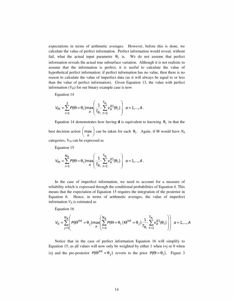
expectations in terms of arithmetic averages. However, before this is done, we calculate the value of perfect information. Perfect information would reveal, without fail, what the actual input parameter iθ is. We do not assume that perfect

information reveals the actual true subsurface variation. Although it is not realistic to assume that the information is perfect, it is useful to calculate the value of hypothetical perfect information: if perfect information has no value, then there is no reason to calculate the value of imperfect data (as it will always be equal to or less than the value of perfect information). Given Equation 13, the value with perfect information (VPI) for our binary example case is now

Equation 14

AavT

PV

i

T

t

ita

aiPI

i

i

,...,1)(1

max)(2

1 1

)( =

θθ=Θ=∑ ∑

= =θ

θ

.

Equation 14 demonstrates how having d is equivalent to knowing iθ in that the

best decision action

amax can be taken for each iθ . Again, if Θ would have Nθ

categories, VPI can be expressed as

Equation 15

AavT

PV

N

i

T

t

ita

aiPI

i

i

,...,1)(1

max)(

1 1

)( =

θθ=Θ=∑ ∑

θ θ

= =θ

.

In the case of imperfect information, we need to account for a measure of reliability which is expressed through the conditional probabilities of Equation 4. This means that the expectation of Equation 15 requires the integration of the posterior in Equation 6. Hence, in terms of arithmetic averages, the value of imperfect information VII is estimated as

Equation 16

AavT

PPV

N

j

T

t

ita

N

i

jia

jII

i

i

,...,1)(1

)|(max)(

1 1

)(

1

intint =

θθ=Θθ=Θθ=Θ=∑ ∑∑

θ θθ

= =θ=

Notice that in the case of perfect information Equation 16 will simplify to Equation 15, as all values will now only be weighted by either 1 when i=j or 0 when

i≠j and the pre-posterior )(int

jP θ=Θ reverts to the prior )( iP θ=Θ . Figure 3

15

demonstrates the components of this equation and how chronologically the geologic parameter iθ is interpreted before choosing the best decision action for that

interpretation. The four values weighted by their posterior value (Equation 6) are explicitly shown for the binary example. The highest weighted value for each interpretation jθ is then chosen for that branch. Finally, VII is the expected value of

these two values, weighted by their respective probability )(int

jP θ=Θ (Equation 7).

Figure 3: Decision Tree depicting the calculations for the Value with Imperfect Information. Chronologically, we can interpret the possibility first (red node) and

then chose the best action (blue node). Again, calculations start from right and proceed left. (1) with the probability that the interpretation is correct or incorrect. (3) Finally, the value with imperfect information (VII) is the expected value of the best

action for each interpreted branch. This is weighted by the probability of each

interpretation being made )(int

jP θ=Θ .

The VOI calculation has now been completed with a single input parameter Θ and two possible outcome values for iθ . We now generalize the calculation of Vprior

and VII to more input geological parameters and their outcomes; we focus on VII as it utilizes the reliability measure. Suppose that a total of M other geologic input parameters are included, which all have outcomes iθ that are mutually exclusive

16

from each other. These additional input parameters can be represented by the vector Θ .

Equation 17

[ ]M1 ,...,ΘΘ=Θ

To distinguish the geologic input parameter and its outcome value from other input parameter outcomes, an additional subscript m is introduced: { }Mii ,...,1

θ where

)(,...,1

mm Ni θ= , Mm ,...,1= , and )(m

Nθ is the number of possible outcomes

(categories) for input parameter mΘ .

For instance, assume two possible additional input parameters such as a variogram model type and the paleo-direction of a lithofacies, represented by 2Θ and

3Θ respectively. Suppose that the variogram parameter 2Θ models three ranges for

the continuity within the lithology classified as low, medium, and high range. On the other hand, the rotation parameter 3Θ for the paleo-direction determines the

orientation of facies as either northeast or southwest. Therefore, the new possible categories will be combinations of all the outcomes of all the included parameters

[ ]321 ,, ΘΘΘ=Θ . For this extended example, }1,3,2{θ would denote the category

where the training image is fluvial, the variogram range is high, and the facies orientation deemed northeast.

With this additional index m denoting from which Θ the samples were drawn, all previous definitions can be extended to include all M input parameters and their respective outcomes. The generalized form of Vprior (Equation 12) is now

Equation 18

{ }( ){ }

{ }

{ }

AavT

PV

M

M

Mii

M

Mii

M

N

i

N

i

T

t

iitaii

aprior ,,1)(

1max

)( )1(

1

,,1

1

,,1

1

1 1 1

,,)(

,, KK

K

K

KK =

θθ=Θ= ∑ ∑ ∑θ θ

θ

= = =θ

.

Most importantly, the total number of categories used for the reliability measure is now

Equation 19

∏=

θ=M

m

mtotal NC

1

)( .

17

Note that in all rigor, this may require M interpretation techniques (hm) for the M geological input parameters. The geophysical method is expected to uniquely distinguish between all these categories. Thus, the Bayesian confusion matrix will be of dimension totaltotal CxC

Equation 20

{ } { } MmNi,jPm

iijj MM,,1,,1)|(

)(,,,,

int11

KKKK ==θ=Θθ=Θ θ ,

such that all unique combinations of { }Mii ,,1 Kθ are represented. Lastly, the

calculation for the value with imperfect information of Equation 16 is modified to include all the combinations of geological parameters and their values as follows:

Equation 21

( )

{ }( )( )

{ } { }( ){ }

{ }( ){ }

AavT

P

PV

Mii

M

Mii

MM

M

M

M

M

M

T

t

iita

N

i

jjii

N

ia

N

j

jj

N

j

II

,,11

|...max

,,1

1

,,1

)1(

1

11

)(

1

1

1

,,)(

1

,,int

,,

1

1

,,int

1

KK

LL

K

K

KKK

K

=

θθ=Θθ=Θ

θ=Θ=

∑∑∑

∑∑

θθθ

θθ

=θ==

==1

We now present an example of a VOI calculation for a synthetic aquifer recharge decision.

3. VOI Example

VOI can be viewed as the interplay of three components: the reliability of the information, the chance of making a poor or suboptimal decision, and the magnitude of the decision. In this section, our results will demonstrate the contribution of this work: a quantitative, repeatable and comprehensive method to obtain such value of information for spatial decision problems accounting for reliability of spatial data. The second and third VOI factors are outside of the scope of this paper and would need to be addressed by sensitivity studies on both the spatial uncertainty modeling parameters as they relate to the decision and the VOI sensitivity to other elements such as the costs and/or values assigned to different outcomes of the decision. Nominal economic values have been chosen for both values and costs. Realistic values could be obtained through experts (e.g. economists), but this economic modeling is not the purpose of this example.

Obtaining a meaningful data reliability will give more confidence in the calculated value of information. Recall that the VOI metric is crucial for stakeholders

18

faced with protection or extraction decisions for assets such as groundwater resources, oil reservoirs, or mineral deposits, where in all cases data collection represents a large expense. To demonstrate this, a synthetic aquifer example, inspired by a real case on the California coast, will demonstrate how this reliability measurement is used in a VOI calculation for a spatial decision with subsurface uncertainty. In our case, artificial recharge is considered to mitigate seawater intrusion, as intrusion leads to an increase in salinity and hence a decrease in usability, in a coastal fluvial aquifer that is critical for farming operations. The spatial decision concerns the location for performing this recharge, if at all, given the uncertainty of the subsurface channel directions, how they affect the success of the recharge actions, and the costs of the recharge operation.

First, the prior uncertainty model is described. Then, alternatives to this decision are established, and the range of outcomes from the combination of models and alternatives are generated. Finally, to illustrate a geophysical data measurement scenario, airborne and land-based transient electromagnetic (TEM) techniques are evaluated for their ability to resolve the channel orientation. We emphasize that this example serves to illustrate the VOI calculation methodology under spatial uncertainty; we will not focus in detail on the geophysics or any economics in the value calculation itself.

3.1. Prior Geological Uncertainty

Only one input geologic parameter (M=1) is used in the example: orientation of

the channels. The prior models )()( θt

z are generated using three possible channel

direction scenarios ( θN =3): dominantly northeast, dominantly southeast and a mix of

both. These three scenarios are deemed equally probable (1

( ) 0.3i

PNθ

Θ = θ = = );

ideally, this prior likelihood for each scenario would come from the expert geologist for any particular area. For each of these three scenarios, 50 Earth models are generated using a channel training image (Figure 4) and the algorithm snesim (Single Normal Equation Simulation) within Stanford’s Geostatistical Earth Modeling Software (SGeMS) [Remy et al, 2009]. snesim is a multiple-point geostatistical algorithm which has a rotation functionality [Strebelle, 2002]. snesim utilizes rotation maps to locally turn patterns of the training image. The angle maps that represent the three channel scenarios and an example 2D realization generated from each are illustrated in Figure 5.

19

Figure 4: Fluvial Training Image; Red = sand facies; Blue=non-sand facies

Figure 5: (A) Example rotation maps and (B) 2D Earth models from snesim for each of the three channel scenarios (80x80X1 cells, 5.3kmx5.3kmx70m, blue=non-

sand facies and red=sand facies)

20

3.2. Decision Actions

Four alternatives to the recharge decision are identified as 1) no recharge, 2) a central recharge location, 3) a northern recharge location, and 4) a southern recharge location. Flow simulation is performed for all combinations: the four recharge options on all the three channel scenarios (specifically the 50 lithology Earth models within each), resulting in a total of 50 x 3 x 4 = 600 flow simulations. The decision tree (Figure 6) visualizes these decision options (blue node) and the possible states of nature.

Figure 6: Decision tree schematic for the prior value of the aquifer recharge example. The red nodes denote the 3 angle scenarios. The blue node denotes the 4

recharge options.

3.3. Value Definition

For this example, we consider that groundwater is used for agriculture. Thus, the volume of freshwater in the aquifer after 10 years, with or without recharge, is equated into potential crop revenue in dollars for farmers. Essentially, if the water in any reservoir cell is below a salinity threshold of 150 ppm (parts per million) of chloride at time=10 years, then the volume of water in that cell (m3) is converted to the production of crop “X” (this is given by the required volume of water to produce

21

1 ton of crop “X”: tons/m3). This can then be equated into dollars by the price of crop “X” ($/ton). For all options where recharge is performed, initial and operational costs of the artificial recharge are subtracted out of the final value (approximately 30% of the average profit for the outcomes without recharge). The resulting value for each recharge-channel direction scenario combination ( )( iav θ ) is seen on the far right of

Figure 6. The prior value (Equation 12) of these possibilities and decision alternatives given the prior uncertainties is $12.47x106 and the value with perfect information (Equation 15) is $12.8x106. Therefore the value of perfect information is approximately $300,000 (VPI – Vprior).

3.4. TEM Reliability

Transient or time-domain electromagnetic (TEM) data is considered to help determine aquifer heterogeneity, specifically the channel orientation. TEM works with a transmitter loop that turns on and off a direct current to induce currents and fields into the subsurface; meanwhile, the larger receiver loop measures the changing magnetic field response of induced currents in the subsurface [Christiansen, 2003]. The data (the magnetic field response in time) must then be inverted to a layered model of electrical resistivity and thickness values which is achieved through geophysical inversion [Auken et al, 2008]. The recovered electrical resistivity can be an indication of the lithology type as clay (non-sand) typically has an electrical resistivity less than 30 ohm-m, whereas sand is usually greater than 80 ohm-m. Therefore, from the TEM measurement, a lithological image can be recovered.

In the prior models )()( θt

z , the channels are represented as sand, and background

facies is non-sand. The orientation of these channels is here deemed, as an illustration, to be the dominant geologic parameter that determines the success of the artificial recharge; consequently, each of the inverted images must be evaluated (interpreted) to determine for the direction of the channels. To achieve this by automatic interpretation (note this is needed because we need to interpret 150 inversion results in terms of channel direction), we calculate the directional variogram maps from the inversion image [Marcotte, 1996]. This analysis is also performed on the original models so that we can compare the “true” channel-direction scenarios with the interpreted ones to obtain the probabilities of Equation 4. Figure 7 shows two examples of the image analysis on both the lithology models and its inversion result, followed by an illustration of the difference of these specifically when a northeast channel orientation was misinterpreted as southeast.

22

Figure 7: Results of image analysis for the angle of maximum correlation. A) Original and inversion results shown for a model (z(θ)) from scenario Northeast. Far right, the locations are shown in red where Northeast is misclassified as Southeast and

in blue where correctly classified. B) Original and inversion results shown for a model (z(θ)) from scenario Mixed. Far right, the locations are shown in red where

Northeast is misclassified as Southeast and in blue where correctly classified.

Recall the underlying goal of this analysis, namely, to determine how well TEM can identify the channel orientation of the original model (i.e. the reliability measure), such that ultimately the value of imperfect information (VII) can be calculated. With all the original models and inversion images, the frequency of misclassification is obtained for both airborne and land-based TEM. The conditional probabilities (Equation 20) for airborne and land-based are represented in Table 1 and Table 2, where the rows and the columns represent the true geologic scenario iθ=Θ and the

interpreted scenario jθ=Θint respectively. In constructing Table 1 and Table 2 two

assumptions were made. First, electrical resistivity was assumed constants for each lithology: sand was assigned 80 ohm-m and non-sand 13 ohm-m. Hence, it was assumed that lithology is the major discriminator in electrical resistivity. Second, for the example problem and for computational reasons, a 1D forward modeling code was used which does not capture the effect of lateral heterogeneity on the TEM measurement.

23

Table 1: Airborne TEM Reliability

Interpreted

Scenario

Mixed Northeast Southeast

Mixed 96% 0% 4% Northeast 0% 98% 2%

Tru

e

Scen

ari

o

Southeast 0% 0% 100%

Table 2: Land-based TEM Reliability

Interpreted Scenario

Mixed Northeast Southeast

Mixed 64% 4% 32% Northeast 24.4% 48.8% 26.8%

Tru

e

Sce

na

rio

Southeast 37.2% 25.6% 37.2%

The two reliabilities of airborne and land-based measurements (Table 1 and Table 2) are quite different. This is due to the difference of in-line measurement separation. For land TEM, in-line measurements are 250m apart as opposed to 50m for the airborne method. Thus, the resolution of channel orientation is decreased for land TEM with fewer locations of measurements. Utilizing the reliability measures of Table 1 and Table 2 in Equation 21, the VOIimperfect (VII – Vprior) for airborne and land-based TEM are ~$260,000 and $0. Compared to VOIperfect ($300,000) the influence of the reliability measure is apparent. Under our assumptions, if the price of acquiring airborne TEM is less than $260,000, then it is deemed a sound decision to purchase this information.

4. Discussion & Conclusions

VOI quantifies how much a new information source would improve our chances of making a better decision than without it. VOI has the potential to be a powerful tool for decision makers who are considering purchasing this information. However, any VOI calculation is only as realistic as the prior model of uncertainty on the studied subsurface heterogeneity as well as the reliability measure of the measurement technique. The methodology presented in this paper is flexible to many prior modeling approaches and is expandable to include many subsurface qualities or features. This work provides a repeatable quantitative and Monte Carlo simulation-based methodology to achieve a reliability measurement based on the resolving power of a particular geophysical technique. Instead of generating many datasets to approximate a posterior distribution, we use these datasets to make interpretations and assess the correctness of all the interpretations, thereby including “geophysical interpretation” as part of VOI. If the geophysical calculation is computationally less

24

expensive than the decision action calculation (which is true in this example since the geophysical forward is 1D and the decision action is 2D flow simulation), then this technique is computationally feasible. With the reliability measure in hand, the decision action calculation is only performed for the prior models and the geophysical reliability measure is used to calculate arithmetic averages for the value of imperfect information. Otherwise, all decision actions A must be performed on all conditioned models (that reflect the information gained from the simulated datasets) in addition to the prior models.

This work attempts to achieve a realistic estimation of VOI by proposing comprehensive prior Earth modeling schemes along with a physics-based reliability measure. However, limitations still exist. To begin a VOI calculation, the possibilities (state variables) affecting the decision must be clearly defined and framed. Howard (1966) recommends a sensitivity study to identify the essential state variables: the uncertain elements that have the greatest influence on a decision outcome. For subsurface problems, this requires coordination between the expert(s) on possible subsurface states and the modelers of the sensitivity study. It is the responsibility of the local geologist to identify what is possible and probable in the subsurface given the location’s depositional and structural history. It is optimistic to assume (especially from the geologist’s point of view) that the subsurface clearly classifies into different categories. However, this is the responsibility of a sensitivity analysis: to identify which subsurface elements are most impacting the decision. Therefore, the prior modeling requires close collaboration between the geologist and the modeler to establish satisfactory geological categories },...,{ 1 Miiθ . Additionally,

the sensitivity study would ideally identify the appropriate categories that must be established for any continuous variable included in the prior modeling.

A significant limitation resides in the interpretation techniques’ ability to classify complicated Earth models. Once rock physics relationships, physics of the measurement and noise are included, it may be difficult or impossible to distinctly classify a geophysical result into one of the initial },,{ 1 Mii Kθ . If the geologic input

parameter of orientation is established with two directions, it is possible that the interpretation could result in a third direction that was not originally represented

( Θ∉Θint ). Sophisticated interpretation techniques are required to analyze multi-dimensional subsurface features. These problems could be alleviated by taking care to only include geologic input parameters that impact the decision outcomes, thus reducing the complexity of the Earth models.

Finally, another significant assumption is that the physics of the geophysical

25

technique is simulated as accurately as possible for the forward modeling )(⋅f .

However 3D modeling and inversion codes are often not available or too CPU demanding to be repeated on a large set of models. This proposed methodology requires

iTCtotal θ× generated forward responses (one for each of the Earth models).

Efficient methods for clustering the Earth models using distance and kernel methods (e.g. Scheidt and Caers, 2009) can help to reduce the computational demands in VOI calculations for spatial decisions.

References

[Auken et al, 2008] Auken, E., Christiansen, A., Jacobsen, L., and Sørensen, K. (2008) A resolution study of buried valleys using laterally constrained inversion of TEM data. Journal of Applied Geophysics, 65: 10-20.

[Bhattacharjya et al, 2010] Bhattacharjya, D., Eidsvik, J. and T. Mukerji, T. (2010) the value of information in spatial decision making, Mathematical Geosciences, 42: 141-163.

[Bickel, et. al, 2006] Bickel, J. E., Gibson, R. L., McVay, D. A., Pickering, S., and Waggoner, J. (2006) Quantifying 3D land seismic reliability and value, Society of Petroleum Engineers Journal, SPE 102340.

[Bickel, 2008] Bickel, J. E. (2008) The relationship between perfect and imperfect information in a two-action risk-sensitive problem, Decision Analysis, 5(3):116-128.

[Bickel & Bratvold, 2008] Bickel, J.E. and Bratvold, R.B. (2008) From uncertainty quantification to decision-making in the oil and gas industry, Energy Exploration & Exploitation 26(5):311-325.

[Bishop, 1995] Bishop, C. (1995) Neural Networks for Pattern Recognition. Oxford University Press, New York.

[Bratvold, et. al, 2009] Bratvold, R.B., Bickel, J.E., and Lohne, H.P. (2009) Value of information in the oil and gas industry: past, present, and future, Society of Petroleum Engineers Journal, SPE 110378.

26

[Caers, 2005] Caers, J.K. (2005) Petroleum Geostatistics. Society of Petroleum Engineers, Texas.

[Christiansen, 2003] Christiansen, A.V., 2003, Application of airborne TEM methods in Denmark and layered 2D inversion of resistivity data: PhD dissertation, University of Århus, Denmark, 136 p.

[Clemen & Reilly, 2001] Clemen, R.T. and Reilly, T. (2001) Making Hard Decisions, second edition. Duxbury Press: Pacific Grove, California.

[Cornell & Newmark, 1978] Cornell, C.A. and Newmark, N.M. (1978) On the seismic reliability of nuclear power plants, ANS Topical Meeting on Probabilistic Reactor Safety, Newport Beach, California.

[Eidsvik et al, 2008] Eidsvik, J., Bhattacharjya, D., and T. Mukerji (2008) Value of information of seismic amplitude and CSEM resistivity. Geophysics, 70(4): R59–R69.

[Feyen & Gorelick, 2005] Feyen, L. and Gorelick, S. (2005) Framework to evaluate the worth of hydraulic conductivity data for optimal groundwater resources management in ecologically sensitive areas. Water Resources Research, 41(3): 13 pp.

[Howard, 1966] Howard, R.A., (1966) Decision Analysis: Applied Decision Theory, Proceedings of the Fourth International Conference on Operational Research, Wiley-Interscience, pp. 55-71.

[Houck, 2004] Houck, R.T. (2004) Predicting the economic impact of acquisition artifacts and noise, The Leading Edge, 23(10):1024-1031.

[Houck & Pavlov, 2006] Houck, R. T. and Pavlov, D. A. (2006) Evaluating reconnaissance CSEM survey designs using Detection Theory, The Leading Edge, 25(8):994-1004.

[Houck, 2007] Houck, R.T. (2007) Time-lapse seismic repeatability—How much

27

is enough? The Leading Edge, 26(7):828-834.

[Marcotte, 1996] Marcotte, D. (1996) Variograms/covariances in the frequency domain via the Fast Fourier Transform (FFT). Computers & Geosciences, 22(10):1175-1186.

[Matheson, 1990] Matheson, J.E. (1990) Using influence diagrams to value information and control, in R.M. Oliver and J.Q. Smith, eds., Influence Diagrams, Belief Nets and Decision Analysis, Wiley, 25-48.

[Mavko, et. al., 1998] Mavko, G., Mukerji, T., and Dvorkin, J. (1998) The Rock Physics Handbook. Cambridge University Press.

[Paté-Cornell & Fischbeck, 1993] Paté-Cornell, M.E. and Rischbeck, P.S. (1993) Probabilistic risk analysis and risk-based priority scale for the tiles of the space shuttle, Reliability Engineering and System Safety, 40(3):221-238.

[Paté-Cornell, 1990] Paté-Cornell, M.E. (1990) Organizational aspects of engineering system safety: the case of offshore platforms, Science, 250:1210-1217.

[Paté-Cornell, 2007] Paté-Cornell, M.E. (2007) Engineering risk analysis: volume 1, MS&E 250A Course Reader, Stanford University.

[Polasky and Solow, 2001] Polasky, S., and Solow, A.R. (2001) The value of information in reserve site selection, Biodiversity and Conservation, 10:1051-1058.

[Raiffa, 1968] Raiffa, H. (1968) Decision Analysis. Addison-Wesley: Reading, Massachusetts.

[Reichard & Evans, 1989] Reichard, E. G., and Evans, J.S. (1989) Assessing the value of hydrogeologic information for risk-based remedial action decisions. Water Resources Research, 25(7):1451-1460.

[Remy et al., 2009] Remy, N., Boucher, A., and Wu, J. (2009) Applied

28

Geostatistics with SGEMS: A User's Guide, Cambridge University Press: New York, NY.

[Ripley, 1996] Ripley, B.D. (1996) Pattern Recognition and Neural Networks. Cambridge University Press: Cambridge.

[Scheidt and Caers, 2009] Scheidt C. and Caers J. (2009) Uncertainty quantification in reservoir performance using distances and kernel methods – application to a West-Africa deepwater turbidite reservoir. Society of Petroleum Engineers Journal, 14 (4):680:692, SPEJ 118740-PA.

[Strebelle, 2002] Strebelle, S. (2002) Conditional simulation of complex geological structures using multiple-point statistics. Mathematical Geology, 34(1):1-26.

[Suzuki and Caers, 2008] Suzuki, S. and Caers, J. (2008) A distance-based prior model parameterization for constraining solutions of spatial inverse problems. Mathematical Geosciences, 40(4):445-469.