Clemson UniversityTigerPrints

All Theses Theses

5-2013

A METHODOLOGY FOR DESIGNINGPERVIOUS BICYCLE LANES FORSTORMWATER MANAGEMENTDonald West IIIClemson University, dwwest@g.clemson.edu

Follow this and additional works at: https://tigerprints.clemson.edu/all_theses

Part of the Civil Engineering Commons

This Thesis is brought to you for free and open access by the Theses at TigerPrints. It has been accepted for inclusion in All Theses by an authorizedadministrator of TigerPrints. For more information, please contact kokeefe@clemson.edu.

Recommended CitationWest, Donald III, "A METHODOLOGY FOR DESIGNING PERVIOUS BICYCLE LANES FOR STORMWATERMANAGEMENT" (2013). All Theses. 1669.https://tigerprints.clemson.edu/all_theses/1669

A METHODOLOGY FOR DESIGNING PERVIOUS BICYCLE

LANES FOR STORMWATER MANAGEMENT

A Thesis

Presented to

the Graduate School of

Clemson University

In Partial Fulfillment

of the Requirements for the Degree

Master of Science

Civil Engineering

by

Donald Wayne West, III

May 2013

Accepted by:

Dr. Nigel B. Kaye, Committee Chair

Dr. Bradley J. Putman

Dr. Leidy Klotz

ii

ABSTRACT

Bicycles have proven to be an efficient and reliable form of transportation in

urban settings. Therefore, the addition of bicycle lanes into the transportation network

could significantly impact and improve the sustainability of our infrastructure by

reducing greenhouse emissions and improving the health of individuals who cycle on a

regular basis. Pervious pavements are an approved (LID) strategy that could potentially

be used to construct these new facilities thereby reducing the quantity of stormwater

runoff and improving the water quality. Practicing engineers need both a design aid and

research supported methods for designing these improvements before they can be fully

implemented throughout the state and country. The data and results presented in this

thesis have accomplished three main objectives: 1) the effects of slope on surface

infiltration rates of pervious pavements due to run-on from adjoining impervious traffic

lanes were analyzed and a design procedure for surface infiltration was presented; 2) the

characteristics of sub-surface flow for multiple slope, flow rate, and discharge weir

conditions were analyzed and a design procedure for the bicycle lane subbase was

presented; and 3) a preliminary investigation of an improved test method was completed

to determine the permeability of pervious materials which could be used for bicycle lane

construction. Three apparatus were constructed for use in these experiments; the bicycle

lane test rig, used to complete the surface and sub-surface flow experiments, along with

two falling head permeameters and two forced flow permeameters used to evaluate

different procedures for measuring the permeability of a porous material. The design

procedures included in this thesis include a method to determine the required bicycle lane

iii

width and hydraulic conductivity required to intercept a design storm flow and a routine

to design a cascading reservoir subbase system to control and infiltrate stormwater

intercepted by the bicycle lane. This thesis does not specifically address the structural

design of the pervious pavement or subbase. Further research is needed to fully evaluate

the effectiveness of current and alternative procedures for determining the permeabilities

of pervious pavements and subbase aggregates. Additionally, further details need to be

addressed for the pervious bicycle lane design including the use of underdrains, the

potential for surface clogging, and the stability of adjacent roadways.

iv

DEDICATION

To Jesus Christ, my Creator, Redeemer, Savior, Shepherd, King, Comforter,

Advocate, Friend – the one true and living God.

v

ACKNOWLEDGMENTS

This material is based upon work supported by the National Science Foundation

under Grant No. 1011478. Any opinions, findings, and conclusions or recommendations

expressed in the material are those of the author and do not necessarily reflect the views

of NSF.

The author would like to thank Mr. Kent Guthrie and Mr. Rick Cotton of the City

of Clemson for providing a summer internship experience. Also, special thanks to Mr.

Michael Horton of Davis and Floyd and Mr. Michael Ulmer of S&ME who served as

external reviewers of this thesis. In addition, the author would like to acknowledge the

following individuals for their helpful contributions, without which this work would not

have been possible:

Dr. Nigel Kaye

Dr. Brad Putman

Dr. Leidy Klotz

Karen Lanning

Martha Zglinicki

Kristi Baker

Will Martin

Andrew Neptune

Rebecca Clark

Danny Metz

Scott Black

Warren Scovil

Murray Fisher

David Lowe

David Christopher

vi

TABLE OF CONTENTS

Page

TITLE PAGE .................................................................................................................... i

ABSTRACT ..................................................................................................................... ii

DEDICATION ................................................................................................................ iv

ACKNOWLEDGMENTS ............................................................................................... v

LIST OF TABLES ........................................................................................................ viii

LIST OF FIGURES ........................................................................................................ ix

CHAPTER

I. INTRODUCTION ......................................................................................... 1

1.1 Literature Review............................................................................... 2

1.1.1 Pervious Pavements ........................................................................ 4

1.1.2 Stormwater Infiltration.................................................................... 9

1.1.3 Clogging of Pervious Pavements .................................................. 16

1.1.4 Hydraulic Modeling ...................................................................... 18

II. MATERIALS APPARATUS ...................................................................... 23

2.1 Coarse Aggregate ............................................................................. 23

2.2 Pervious Concrete ............................................................................ 27

2.3 Soil ................................................................................................... 31

2.4 Experimental Apparatus................................................................... 31

2.4.1 Bicycle Lane Test Rig ................................................................... 31

2.4.2 Falling Head Permeameter ............................................................ 43

2.4.3 Forced Flow Permeameter ............................................................ 47

III. SURFACE FLOW EXPERIMENTS ........................................................... 53

3.1 Model Development......................................................................... 53

3.2 Steady State Solution ....................................................................... 55

3.3 Surface Flow Experiments ............................................................... 57

3.4 Surface Flow Experiment Results .................................................... 59

3.5 Discussion and Conclusions ............................................................ 62

vii

Table of Contents (Continued)

IV. SUB-SURFACE FLOW EXPERIMENTS.................................................. 67

4.1 Model Development......................................................................... 69

4.2 Test Rig Calibration ......................................................................... 75

4.2.1 Calibration Test Results ................................................................ 77

4.3 Sub-Surface Flow Experiments ....................................................... 79

4.4 Sub-Surface Flow Experimental Results ......................................... 82

4.5 Discussion and Conclusions ............................................................ 85

V. PERMEABILITY EXPERIMENTS ............................................................ 90

5.1 Permeameter Theory ........................................................................ 90

5.2 Results and Discussion .................................................................... 92

5.3 Conclusions .................................................................................... 103

VI. SUMMARY AND CONCLUSIONS ........................................................ 104

REFERENCES ............................................................................................................ 108

viii

LIST OF TABLES

Table Page

2.1 Product specifications for aggregate materials obtained

from Vulcan Materials Liberty, South Carolina

quarry (Vulcan Materials 2013) ............................................................. 23

2.2 Sieve analysis results for No. 57 stone. ....................................................... 24

2.3 Hydraulic Conductivity of No.57 stone. ...................................................... 25

2.4 Sieve analysis results for 89M stone. ........................................................... 26

2.5 Pervious Concrete Properties ....................................................................... 28

3.1 Infiltration rates determined by ASTM C 1701. .......................................... 57

3.2 Equivalent surface run-on flow rates. .......................................................... 59

3.3 Intrinsic Permeability and Hydraulic Conductivity for

equivalent infiltration rates determined in

accordance with ASTM C1701. ............................................................. 60

4.1 Simulated rainfall intensities for calibration tests. ....................................... 75

4.2 Calibration test results.................................................................................. 77

4.3 Metered flow equivalents for sub-surface flow test. .................................... 80

5.1 Results of porosity and falling head permeameter testing. .......................... 93

5.2 Curve fitting results for forced flow permeameter experiments. ................. 94

5.3 Estimates of permeability calculated from forced flow

permeameter results using cF equals 0.55. ............................................ 96

5.4 Estimates of permeability calculated from forced flow

permeameter results using cF equals 2.03. ............................................ 97

5.5 Individual drag coefficient determined for each cylinder. ........................... 99

ix

LIST OF FIGURES

Figure Page

1.1 Potential bicycle lane grading patterns. ....................................................... 13

1.2 Natural Resource Conservation Service 24-hour storm intensity curve. ..... 19

1.3 Hyetograph of maximum intensity storms for South

Carolina using the Natural Resource Conservation

Service Type II 24-hour duration storm for the 2,

10, and 100 year design storm event. ..................................................... 20

1.4 Sampling of potential pervious pavement bicycle lane

design parameters................................................................................... 21

2.1 Particle-size distribution curve for No. 57 stone. ........................................ 25

2.2 Particle-size distribution curve for No. 89M stone. ..................................... 27

2.3 Bicycle lane test rig cross-section. (End View) ........................................... 32

2.4 Bicycle lane test tank showing waterproofed interior

and trays to capture outflow from aggregate and

pervious concrete layers. ........................................................................ 33

2.5 No. 57 stone drainage layer and geotextile fabric

installation. ............................................................................................. 34

2.6 Geotextile fabric and placement of Cecil soil. ............................................. 35

2.7 Moisture barrier and manometer tube installation before

No. 57 stone placement. ......................................................................... 36

2.8 Pervious concrete placement on compacted No. 57

stone base. .............................................................................................. 37

2.9 Leveling the surface of the pervious concrete slab. ..................................... 38

2.10 Completed tank with soaker hose rainfall system

installed. ................................................................................................. 39

x

List of Figures (Continued)

Figure Page

2.11 Completed run-on weir used for surface flow

experiments. ........................................................................................... 40

2.12 Surface flow experimental setup. ................................................................. 41

2.13 Surface flow experiment measurements. ..................................................... 41

2.14 Schematic diagram of falling head permeameter. ........................................ 44

2.15 Falling head permeameter used to determine hydraulic

conductivity of pervious concrete cylinders and No.

57 aggregate. .......................................................................................... 45

2.16 Pervious concrete cylinder prepared for testing in

falling head or forced flow permeameter. .............................................. 46

2.17 Schematic diagram of forced flow permeameter. ........................................ 49

2.18 Forced flow permeameter apparatus. ........................................................... 50

3.1 Schematic diagram of surface flow model. .................................................. 54

3.2 Plexiglas weir used to simulate sheet flow across the

pervious pavement surface. .................................................................... 58

3.3 Plot of measured infiltration distance versus flow rate

per unit width, q0, for pavement slopes of 0%

(blue), 5% (red), and 10% (green). The same five

flow rates were tested for each slope; however, q0

varies due to flow width contraction. The solid line

represents model results for hydraulic conductivity,

K, equal to 0.0064 m/s, and the dashed line

represents K equal to 0.0103 m/s. .......................................................... 62

3.4 Pervious bicycle lane design section............................................................ 64

4.1 Schematic diagram of sub-surface flow model. ........................................... 67

4.2 Aggregate base layer control volume. ......................................................... 70

xi

List of Figures (Continued)

Figure Page

4.3 Image of calibration testing. Red food coloring was

used to enhance the resolution of the water level

inside manometer tubes. Photos were taken at

regular intervals to determine the change in depth of

water within the aggregate layer over time. ........................................... 76

4.4 Plots of water surface elevation (y) versus elapsed time

for each of five calibration tests. ............................................................ 78

4.5 Outlet control weir at downstream outlet of bicycle lane

test rig..................................................................................................... 81

4.6 Sub-surface flow test image for experiment with

slope=0.02, i = 295 mm/hr [2.5 GPM], Q =

18.9*10-5

m3/s [3.0 GPM], and weir height = 114

mm [4.5 in.]............................................................................................ 82

4.7 Plot of measured results of experiment shown in Figure

4.6. Datum, z=0 is assumed to be the bed elevation

at the base of the weir. Boxes indicate the actual

measured data points. ............................................................................. 83

4.8 Plot of Total Flow Rate (Qt) versus H for all sub-

surface flow experiment observations with water

surface elevation greater than weir elevation. H at

the weir plotted as squares and H 152 mm [6 in]

upstream plotted as diamonds. The solid line

represents the solution to the theoretical sharp

crested, rectangular weir equation (4.1.14) adjusted

for the aggregate porosity and the dashed line

represents the solution of the standard rectangular

weir discharge equation (4.1.12). ........................................................... 84

xii

List of Figures (Continued)

Figure Page

4.9 Pervious bicycle lane subbase reservoir routing

diagram. ................................................................................................. 85

4.10 Schematic diagram of single bicycle lane subbase

reservoir cell........................................................................................... 87

5.1 Forced flow permeameter quadratic fit results for

cylinders 1-4........................................................................................... 95

5.2 Permeability results for forced flow permeameter (bars)

and falling head permeameter test (squares and

circles). Square symbols represent results of

Darcy’s Law and circles represent the solution of

the Darcy-Forchheimer equation using the

optimized drag coefficient, cF =2.03. ..................................................... 98

5.3 Plot of drag constant and porosity for pervious concrete

cylinders porosity values plotted as squares and

drag constant values plotted as circles. The red

circles indicate the porosity values for cylinder

numbers 2, 5, and 9 which produce extreme

differences in permeability estimates for force flow

permeameter experiments as seen in Figure 5.2. ................................. 100

5.4 Relationship of drag coefficient to porosity for cylinder

numbers 1-12. ...................................................................................... 101

5.5 Relationship of drag coefficient to permeability for

cylinder numbers 1-12. ........................................................................ 101

5.6 Permeability results for forced flow permeameter (bars)

and falling head permeameter test (squares and

circles) with outliers removed. Square symbols

represent results of Darcy’s Law and circles

represent the solution of the Darcy-Forchheimer

equation using calculated cF values. .................................................... 103

CHAPTER ONE

INTRODUCTION

Bicycles have proven to be an efficient and reliable form of transportation in

urban settings. However, very few cities in South Carolina or the United States have

dedicated bicycle lanes included in their transportation infrastructure network. Most of

our streets and highways are designed for primary use by single occupant vehicles and

freight trucks. Sansalone et. al. (2008) states that as much as 60% of the world’s

population is expected to live in urban settings by the year 2025; if so, the addition of

bicycle lanes into the transportation network could significantly impact the sustainability

of our urban infrastructure.

Additionally, the construction of these bicycle lanes with pervious pavements, a

recognized low impact development (LID) technique, would both reduce the quantity of

stormwater runoff and improve the quality of stormwater entering the state’s many lakes,

oceans, rivers, streams, and other wetlands. Oftentimes the benefits of using pervious

pavements are overlooked by designers of paved surfaces due to the skepticism of owners

and regulators over the long-term performance of pervious pavements, favoring instead

traditional storm sewer systems which capture stormwater runoff and discharge it to

surface waters downstream. Other factors, including the lack of technical guidelines for

installation and maintenance for pervious pavements, have resulted in some failures of

past installations (Eisenberg 2010). Practicing engineers need both a design aid and

research supported methods for designing these improvements before they can be fully

implemented throughout the state and country.

2

The use of pervious bicycle lanes could have significant impact on shaping the

urban landscape in generations to come. Pilot projects have been constructed, including

one located in the city of Olympia, Washington (Tosomeen 2008). However, the design

methods for these practices are not clearly specified, nor are they experimentally verified.

A rigorous study is needed to establish a set of best practices and design guidelines to

properly account for the hydrologic benefits of these structures, to give credibility to their

use, and to ensure they comply with current stormwater regulations.

1.1 Literature Review

Bicycles are becoming an increasingly popular sustainable mode of transportation

on college campuses and in urban environments. Providing infrastructure to

accommodate this alternate form of transportation will become increasingly necessary in

the coming years as citizens continue to flock from rural settings to larger cities. As

much as 60% of the world’s population is expected to live in urban settings by the year

2025 (Sansalone et al. 2008). Improved facilities for cyclists will lead to increased

ridership and decrease the environmental footprint of automobiles powered by carbon

based fuels.

Like cars, bicycles are well suited to hardened, smooth riding surfaces. These

surfaces are typically impervious and increase the stormwater runoff from developed

sites, an ever increasing problem and unsustainable practice in urban settings. Impervious

areas typically account for more than 60% of land area in metropolitan districts

(Sansalone et al. 2008). Pervious pavements can be used to provide additional lanes for

cyclists without increasing the volume of stormwater runoff.

3

Several concerns with the use of pervious pavements must be considered when

designing cycling facilities to ensure rider satisfaction and use of the designated lanes.

Cyclists in urban districts tend to prefer narrow road tires over wider, harder to pedal,

ones best suited for off-road use. Therefore, pervious pavements must be designed to

provide a suitable riding surface free of large voids which could trap or puncture bicycle

tires. The pavement should also provide a smooth riding surface and not produce excess

noise while riding across the surface.

Regardless, pervious concrete pavements provide a potential solution to improve

current cycling facilities. This material allows water to freely drain through its surface,

unlike traditional pavements, decreasing the total runoff and helping to improve overall

stormwater quality. Multiple studies conclude that urban stormwater runoff is the largest

source of pollution in coastal waters in the USA (Burton and Pitt, 2002) (Siriwardene et

al. 2007). This is due in large part because runoff containing sediments and chemicals

deposited by vehicles is not filtered before being discharged into surface waters. Pervious

pavements and their underlying soils can filter these contaminants and improve

downstream water quality.

The lack of a design standard for pervious pavement applications as a stormwater

management tool make it difficult for designers to fully utilize the hydrologic benefits

provided by these systems. Many times, the benefits of using pervious pavements are

ignored and not considered during design; instead designers prefer to use traditional

storm sewer systems as they easily fulfill the requirements of design regulations. Other

factors, including the lack of technical guidelines for construction and maintenance for

4

pervious pavements, have resulted in some failures of past installations (Eisenberg 2010).

A research supported design standard is critical to ensure that new sustainable solutions

such as pervious pavements can replace traditional designs. Any design standard must

address the four main criteria groups common to all pervious pavement applications

which are regulatory requirements, soil conditions, site conditions, and installation and

maintenance concerns (Eisenberg 2010). According to Pitt and Clark, sustainability in

stormwater management requires the use of an appropriate combination of control

practices (Pitt and Clark 2008). A systems approach rather than a one size fits all linear

approach should be employed to address the four specific criteria listed above.

An experimentally verified design guideline would allow designers to further

implement pervious pavements into projects and properly account for their hydrologic

benefits. According to Dietz, “It appears that engineers do not have a consistent design

tool that can credit the runoff reductions that LID components can provide, that is also

based on research results” (Dietz 2007). Standards should address means of quantifying

the benefits of various practices and suggest best practices for their use based on verified

experimental results. Also, the water quality benefits of pervious pavement systems

should be documented and emphasized to complement its water quantity control benefits.

Before defining the scope of this thesis, it is prudent to include a brief discussion

of pervious pavements and stormwater infiltration practices.

1.1.1 Pervious Pavements

Pervious pavements allow water to freely flow through their surface and structure

due to the absence of the fine aggregates, or sands, that are present in traditional concrete

5

and asphalt mixes. Various properties of the concrete or asphalt mix and construction of

the pervious pavement affect its ability to infiltrate water. It is important to understand

which properties best describe the performance of the final product. According to Luck et

al., density and porosity are key indicators of the hydrologic performance of pervious

pavements (Luck et al. 2006).

Pervious pavements must be designed to structurally carry the loads applied to

them by the vehicles travelling on their surface. Currently, pervious pavements are

recommended for use in parking areas, driveways, shoulders, medians, sidewalks, and

small residential streets (Sansalone et al. 2008). However, they are typically not used for

mainline highways where large trucks with high axle loads commonly travel. Saturation

of the subgrade beneath these travel ways is also a major concern as it can degrade the

structural integrity of the roadway. Pervious concrete pavements are typically suitable for

light traffic without a base course underneath and are more than sufficient for bicycle

loads (Ferguson 1994). Typically, a base course will be included when the runoff storage

need exceeds the storage capacity of the pervious pavements or the pavement needs

structural support beyond that provided by the subgrade.

Parking lots, emergency access, and other travel ways used only periodically are

candidates for pervious pavement applications. Additionally, pervious pavements can be

used to structurally improve existing soils without increasing the impervious area. The

greatest contributor to increased runoff and pollution is the addition of impervious ground

covers and buildings which disrupt the natural hydrologic cycle. According to Ferguson,

pervious portland cement concrete stabilizes soils and promotes infiltration (Ferguson

6

1994). The infiltration of runoff into the underlying soils decreases the runoff and

pollutants entering surface waters downstream.

Similarly, a pervious pavement system can be designed to intercept stormwater

runoff alongside streets in urban settings. The goal here is to use the pervious surface in

the same manner that curb inlets and grates are used to remove runoff from gutters.

Currently, storm sewer system design is primarily governed by inlet efficiency and pipe

capacity. The pervious concrete surface could be considered as one continuous grate

opening inlet, replacing the need for catch basins which transfer the runoff to

underground pipes, and possibly reducing the required capacity of underground pipes.

Hydrologic design of pervious concrete stormwater systems however, is primarily

controlled by the infiltration properties of subgrade soils and the storage volume of the

subbase material (Schwartz 2010). Schwartz offers a procedure for the consistent design

of pervious concrete stormwater management systems using an effective NRCS curve

number method that incorporates freeze-thaw risk and timely drawdown of subbase

storage (Schwartz 2010). Though this method attempts to quantify the runoff from

pervious pavements in terms of a commonly used calculation method, it is difficult to

account for variations in mix design, base material, and native soil characteristics.

Pervious concrete pavements also promote runoff reduction by various physical

processes whose benefits are often overlooked. Capillary action, diffusion, and increased

evaporation potential are a few important physical processes often overlooked in pervious

pavement feasibility studies for Low Impact Development techniques (Matel 2010).

7

Consequently, many pervious pavement designs are overly conservative and, therefore,

not cost effective.

Water quality improvement is likely the most important benefit of using pervious

pavements. Research has shown that pervious pavements are effective at removing

contaminants, including sediments and heavy metals from stormwater runoff, and provide

other key environmental benefits. Pervious concrete restores the hydrologic cycle,

leaches calcium and alkalinity and reduces thermal pollution (Sansalone et al. 2008).

Traditionally, municipal separate storm sewer systems (MS4s) collect runoff from

impervious surfaces; transfer the runoff to into pipes or channels; and discharge the

runoff directly to surface waters.

Replacing traditional curb and gutter stormwater collection structures with

pervious pavement systems can greatly reduce the amount of nutrients entering

downstream surface waters. Field surveys in North Carolina indicate significant

reductions in pollutant concentrations including Total Kjeldahl Nitrogen, Ammonium-N,

Total Phosphorus, and Zinc with the use of pervious pavements (Bean et al. 2007b).

Promoting infiltration of the runoff into the underlying soils, instead of transferring

runoff directly to storm sewers, allows biological processes to filter and degrade

contaminants before returning them to groundwater sources. It is important to ensure that

a sufficient amount of soil is present between the bottom of the excavation and the water

table to prevent contamination of groundwater sources.

Field surveys of pervious pavement systems have demonstrated their

effectiveness when used as part of a stormwater management system. Field surveys in

8

North Carolina indicated that proper siting over undisturbed sandy soils, large storage

volumes, and clean pavement surfaces with minimal fines increase the effectiveness of

pervious pavements (Bean et al. 2007b). As with any LID technique, it is important to

establish the use of pervious pavement as a part of the overall basis of design. Proper

planning, construction, and maintenance are essential to effective performance of

pervious pavement systems. Field surveys indicate that proper siting and maintenance are

essential to maintain high surface infiltration rates (Bean et al. 2007a). Certainly, these

planning, design, construction, and maintenance issues must all be considered for

pervious pavement bicycle lanes to be appropriately incorporated into the roadway

system.

Further testing is necessary to determine the effectiveness of these practices for

various site conditions. Field studies provide observations on how pilot projects are

performing long-term; however, they offer little guidance on the methodology which was

used to design individual sites. Also, many techniques currently used to quantify the

benefits of pervious concrete, including those given by Schwartz, are solely based on

theory and not experimentally verified. Many studies have been performed on the

properties of pervious pavement; however, more research focused on the use of pervious

pavement in various systems is necessary to determine its applicability.

Pervious concrete is a unique material that requires certain considerations which

vary from typical pavements. Installation requires specialized techniques that can be

problematic for inexperienced construction crews. Pervious concrete can also require

regular maintenance as excessive sediments can cause clogging of the surface and

9

decrease its ability to pass water through its pores. Regular maintenance restores

hydraulic conductivity and removes pollutants from the pavement structure (Sansalone et

al. 2008). A life cycle cost analysis is necessary to completely characterize the cost to

benefit ratio of replacing current stormwater infrastructure with pervious pavement

practices.

Current applications for pervious pavements assume vertical infiltration on near

level sites and determine storage needs based on peak runoff reduction requirements.

This fact presents a significant problem for applications where pervious pavements are to

be used along roadways, or other vertical alignments, where significant slopes might be

encountered. Current research is inconclusive whether infiltration rates increase or

decrease as slope angle increases; therefore, it is necessary to determine the effects of

slope on infiltration rates for pervious pavement surfaces (Chen and Young 2007; Essig

et al. 2009). The pervious pavement, aggregate subbase, and the existing subgrade are all

elements of the pervious pavement systems that must be considered to evaluate the

benefit of using a pervious pavement system.

1.1.2 Stormwater Infiltration

Infiltration is the process of water passing through the ground surface. This

process restores groundwater, filters contaminants, and minimizes erosion in receiving

streams. Traditional storm sewer systems often eliminate natural infiltration creating

erosion and contamination of receiving creeks and streams. A pervious pavement bicycle

lane system could store stormwater runoff from the road surface until it is able to

infiltrate into underlying soils, returning the area to a near natural condition. Pervious

10

pavements have been incorporated with infiltration basins and shown to perform well

hydrologically without negatively affecting groundwater at Villanova University

(Kwiatkowski et al. 2007). A bicycle lane paved with pervious concrete would act as a

hybrid infiltration trench, or a linear infiltration basin, which is one type of LID

technique.

Infiltration practices, including trenches and basins, have proven to be an

effective means of managing stormwater runoff in small watersheds. Infiltration practices

are structural elements that retain runoff onsite until it can percolate into the ground to

recharge groundwater systems below grade (Ferguson 1994). Infiltration reduces

stormwater runoff, decreases pollutant loads on receiving waters, and replenishes

groundwater sources. Stormwater discharged from sub-surface groundwater can replenish

streams without causing flushing or erosion which typically occurs when stormwater is

discharged directly to surface waters (Ferguson 1994).

Infiltration practices are typically large excavations filled with washed open-

graded aggregate having a large void space good for passing and storing runoff. The base

course for typical pervious pavement applications is sized for storage capacity; the

thickness of base material is increased to provide additional storage to meet the

requirement. Many aggregate gradations are acceptable for pervious base material, but all

aggregates used in reservoirs must be open-graded and washed to minimize fine

sediments which could reduce the void space within the base layer (Ferguson 1994).

Aggregate gradations which have higher void ratios once compacted are best suited for

11

infiltration practices as they decrease the total volume of material needed to create the

necessary storage volume.

Infiltration occurs best on level ground where water is unable to run out of the

porous matrix of the subgrade or infiltration practice. Understandably, pervious

pavements are easily adapted to parking lots where they are used to cover large flat areas

and replace traditional impervious pavements. The usual rule of thumb is to limit the use

of pervious pavements to slopes less than or equal to 5%. This poses a serious issue

where a bicycle lane is to be aligned along a roadway with a significant vertical

alignment. Ferguson suggests that pervious pavements designed for sloping areas be

planned so that the system includes flat reservoir areas connected by sloping pavement

sections (Ferguson 1994). The challenge on sites with significant grades is to prevent

infiltrated water from re-surfacing downslope due inadequate storage capacity beneath

the pavement surface.

Figure 1.1 includes different options for configuring the subgrade and base layer

to minimize the effects of slope on a pervious bicycle lane system. Figure 1.1(a) depicts

the simplest configuration where the subgrade is cut parallel to the finished grade

requiring the least amount of aggregate base which can be spread in a uniform layer. This

is likely the worst scenario as the permeability of the aggregate base is the only resistance

to the flow of water downhill. An improvement to this system would be the addition of

small weirs located at certain intervals along the slope Figure 1.1(b) which would create

small reservoirs of water thereby reducing the amount of water reaching the base of the

slope. Figure 1.1(c) shows terraced reservoir areas similar to those proposed by Ferguson;

12

this system would require additional labor to construct and additional aggregate to

maintain the finished grade. Finally, Figure 1.1(d) produces the advantage of creating

13

Figure 1.1: Potential bicycle lane grading patterns.

14

small reservoir areas with flat bottoms which both reduce the quantity of water flowing to

the base of the hill and promote infiltration on flatter areas.

Infiltration rates can be affected by many factors other than the slope including,

soil type, compaction, season, and antecedent moisture condition in the soil. Infiltration

rates vary by season and temperature; therefore, infiltration practices should be sized to

meet the design efficiency during the time with the lowest infiltration rate (Emerson and

Traver 2008)(Horst 2011). Using infiltration rates from published soil maps, without field

test verification, can lead to large errors in infiltration rate calculations (Pitt et al. 2008).

Field testing and proper planning will be essential to the success of using infiltration

practices as the primary stormwater management system.

The composition of underlying soils is the main factor affecting infiltration rates.

Non-cohesive sandy soils have high infiltration rates allowing water to quickly flow

through the open pore space, but infiltration rates can be affected by soil compaction. The

degree of compaction is an important and often overlooked variable of steady state

infiltration rates in urban soils (Pitt et al. 2008). It is critical that excess compaction due

to construction activities is limited so that natural infiltration rates are not compromised.

Water flows much slower through cohesive clay and silt soils. Dreelin argues that

pervious pavement systems can be effective at infiltrating runoff even in clay soils with

slow infiltration rates (Dreelin et al. 2006). In these situations, it may be necessary to use

underdrains in combination with traditional storm sewers to manage runoff which cannot

be infiltrated in sufficient time.

15

Infiltration practices must be properly sized to retain stormwater runoff and allow

time for infiltration of the water into the native soil. Infiltration practices can be sized to

fulfill several purposes including 1) infiltration of entire inflow volume, 2) to infiltrate

the difference in pre-development and post-development runoff, 3) to infiltrate a fixed

amount of runoff regardless of storm, or 4) to reduce outflow to a given rate (Ferguson

1994). Stormwater collection systems along roadways are designed to limit the spread of

ponded water within the travel lanes. The allowed spread varies depending on the type of

road and volume of traffic (Federal Highway Administration 2009). Sizing of infiltration

practices must not result in underestimation of storage volume, and correct sizing is site

specific for soil and watershed characteristics (Ferguson 1994).

The infiltration practice should be sized so that the void space within the

aggregate is equal to or greater than the volume of runoff produced by the design storm

event. The hydraulic capacity is equal to the volume of the voids, which is equal to the

volume of the basin multiplied by the void content. Void content is typically 0.38-0.40

for open graded crushed stone (Ferguson 1994). The volume of water which must be

stored is dependent on local codes, the choice of design storm event, and soil infiltration

rates.

Perforated pipes could be used to create larger void spaces within the infiltration

practice if necessary. These pipes contain holes or slots which allow water to pass, but

are small enough to prevent aggregates from entering when installed properly. Burying

perforated pipes creates a reservoir system and increases the available storage below

ground (Ferguson 1994). Large pipes are already being used for underground detention

16

ponds, storing water in the large void, and slowly releasing the stored water to other

conduits or to groundwater. This delay of flow could potentially allow designers to

decrease the size of onsite and downstream conduits as well as prevent surpassing the

capacity of existing downstream systems.

1.1.3 Clogging of Pervious Pavements

Clogging is a leading cause of poor performance for pervious pavements and

infiltration practices. Oftentimes, designers must include traditional stormwater collection

systems along with pervious pavement systems to ensure proper functioning of the paved

facility in the event that the pavement becomes permanently clogged, often leading to

higher cost of construction compared to traditional design. Consequently, it becomes

difficult to justify the use of pervious pavements on cost alone. Approximately one-third

of a total 207 infiltration practices surveyed by Lindsey et al. (1992) were not functioning

due to clogging (Siriwardene et al. 2007). Ensuring that appropriate measures are

implemented to prevent clogging and provide proper maintenance is essential to prevent

flooding. This fact may limit the use of infiltration practices along major roadways;

however, they may still be well suited for use in urban environments.

Several factors can affect the clogging rate of infiltration practices including the

volume of flow, the frequency of storm events, and the concentration of sediments in the

runoff. Siriwardene et al. concluded that the clogging rate of infiltration practices

increases with variable inflow and regular emptying (Siriwardene et al. 2007). These

observations are troubling because storm events vary both in time and intensity, and it is

necessary that these practices empty in a timely manner to prevent the promotion of

17

undesirable vectors including mosquitos and other pests. This requirement is known as

drawdown time and is often stipulated in local regulations.

Two mechanisms of clogging are of particular interest when considering a

pervious bicycle lane system: clogging of the pervious pavement surface and sub-surface

clogging which decreases the rate of exfiltration to the underlying native soil. Sub-

surface clogging is prone to occur at the limits of excavation, between the storage layer

and the native soil. According to Siriwardene, the clogging layer in infiltration practices

tends to form at the interface between filter and soil (Siriwardene et al. 2007). Geotextile

fabrics are often used to line infiltration trenches to prevent fine sediments from

migrating into the storage, or base, layer reducing the void ratio of the aggregates, or vice

versa to prevent migration of the stone. These fabrics should be carefully selected to

prevent premature clogging of the infiltration practice. Little can be done in terms of

remediation, or rejuvenation, for infiltration practices located on sites prone to this type

of clogging.

Surface clogging of pervious pavements is the second clogging mechanism of

interest if pervious pavements are to be used to infiltrate stormwater as part of the bicycle

lane system. Clay, or cohesive, soils are often recognized for their ability to fill in the

pores of pervious pavement reducing their hydraulic conductivity. Various procedures

have been presented for laboratory tests to observe or predict the reduction in hydraulic

conductivity due to clogging of pervious pavements (Coughlin et al. 2012; Deo et al.

2010; Haselbach 2010). Typically, these procedures utilize a form of falling head

18

permeability test performed in a cyclic process to simulate multiple storm and surface

drying events comparable to field conditions.

1.1.4 Hydraulic Modeling

Hydraulic modeling can be thought of as the procedure used to determine the

impact of storm events. There are several different methods used in engineering practice

to model the flow of stormwater runoff and aid in the design of stormwater infrastructure.

These include the Natural Resource Conservation Service TR-55 method, the Rational

Method, and the Natural Resource Conservation Service Runoff Curve Number method.

These traditional methods are not well suited to address the benefits of pervious

pavements or other LID techniques as they are mainly concerned with reducing the peak

discharge and flood control. Often, regulations are concerned with the runoff produced by

the 2, 10, and 100 year design storm events, but these vary by jurisdiction, facility type

and purpose. These models assume that conveyance either occurs overland on the ground

surface or through networks of channels, inlet structures, and pipes. These traditional

methods must be modified to properly characterize the performance of a pervious

pavement bicycle lane system.

The hydraulic flow model must combine overland and sub-surface water flow

parameters to simulate flow over the roadway surface and runoff infiltrating through the

pervious pavement bicycle lane. These processes occur simultaneously and the flow

model must account for simultaneous inflow and outflow relationships. The kinematic

wave model for overland flow and the Green and Ampt infiltration model for sub-surface

flow have been suggested for this coupled analysis for soils on slopes (Paige 2002);

19

(Stone 1992). Additionally, Akan suggests a procedure to size stormwater infiltration

structures which couples the infiltration storage equation with the Green-Ampt

infiltration equation to determine the maximum water depth and storage time (Akan

2002).

Regardless, if a pervious pavement bicycle lane system is to be considered to

replace or reduce the need for traditional storm sewer channels and pipes, its performance

must be quantified based on the accepted design storm events. The State of South

Carolina defines the design storm event using the Natural Resource Conservation Service

Type II or III 24-hour storm distribution, as shown in figure 1.2.

Figure 1.2: Natural Resource Conservation Service 24-hour storm intensity curve.

20

The South Carolina Department of Health and Environmental Control (SCDHEC)

provides precipitation values for all design storm events, (return periods of 1, 2, 5, 10, 25,

50, and 100 years) for each of the counties within the borders of South Carolina.

Additionally, multiple values are included for counties that include more than one distinct

region exhibiting different hydrologic characteristics. Figure 1.3 shows the hyetograph

with the maximum rainfall intensity for the 2, 10, and 100 year storm event found in the

state of South Carolina. These maximum intensities represent the worst case design

conditions for South Carolina.

Figure 1.3: Hyetograph of maximum intensity storms for South Carolina using the

Natural Resource Conservation Service Type II 24-hour duration storm for the 2, 10, and

100 year design storm event.

21

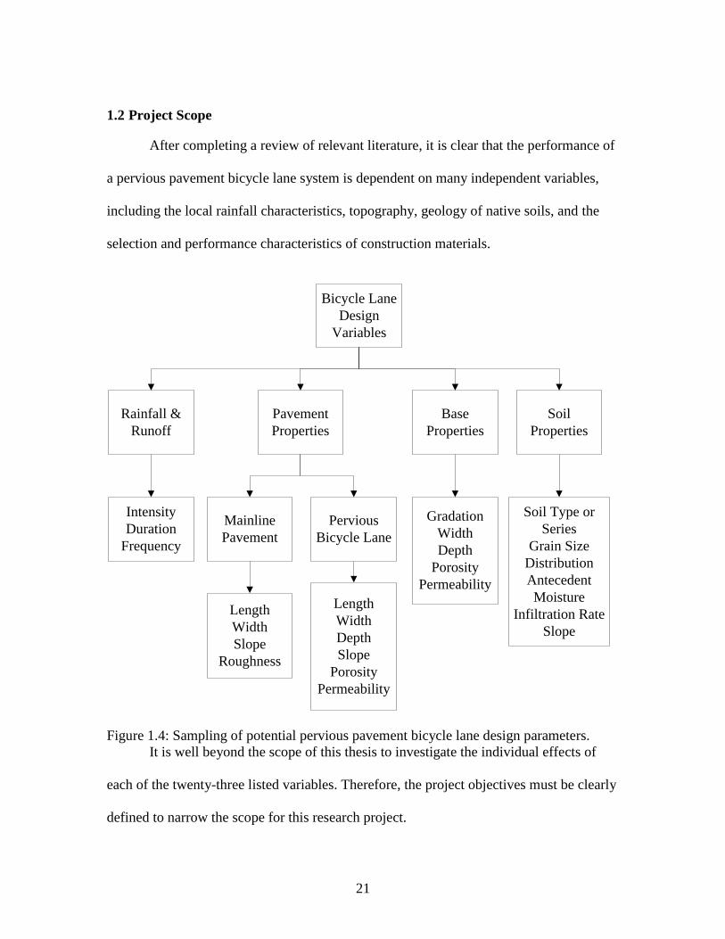
1.2 Project Scope

After completing a review of relevant literature, it is clear that the performance of

a pervious pavement bicycle lane system is dependent on many independent variables,

including the local rainfall characteristics, topography, geology of native soils, and the

selection and performance characteristics of construction materials.

Bicycle Lane

Design

Variables

Pavement

Properties

Rainfall &

Runoff

Base

Properties

Soil

Properties

Mainline

Pavement

Pervious

Bicycle Lane

Intensity

Duration

Frequency

Length

Width

Slope

Roughness

Length

Width

Depth

Slope

Porosity

Permeability

Gradation

Width

Depth

Porosity

Permeability

Soil Type or

Series

Grain Size

Distribution

Antecedent

Moisture

Infiltration Rate

Slope

Figure 1.4: Sampling of potential pervious pavement bicycle lane design parameters.

It is well beyond the scope of this thesis to investigate the individual effects of

each of the twenty-three listed variables. Therefore, the project objectives must be clearly

defined to narrow the scope for this research project.

22

The project objectives for this study are as follows:

1. Determine the effects of slope on surface infiltration rates of pervious pavements

due to run-on from adjoining impervious traffic lanes.

2. Determine the characteristics of sub-surface flow for multiple slope, flow rate,

and discharge weir conditions.

3. Undertake a preliminary investigation of an improved test method to determine

the surface clogging potential of pervious pavements for various soil types and

grain size fractions.

23

CHAPTER TWO

MATERIALS APPARATUS AND PROCEDURES

Several different materials were used throughout the course of this project both as

test specimens and to construct the three apparatus used in conducting the experiments.

The bicycle lane test rig is an approximately three feet by seven feet pervious bicycle

lane model containing soil, aggregates, and a pervious concrete slab. The permeameter

and surface clogging test rigs were designed to test pervious concrete cylinders or loose

materials on a smaller scale. These apparatus will be discussed in more detail in section

2.4.

2.1 Coarse Aggregate

Two types of coarse aggregate, No. 57 and 89M, were utilized for the

construction of the bicycle lane and pervious concrete cylinders. All aggregates,

approximately one cubic yard each, for this project were donated by Vulcan Materials in

Liberty, South Carolina. With the exception of drying, these aggregates were used in the

condition as received from the supplier and no further modification was made. The

material properties of the stone obtained from the Liberty quarry are listed in Table 2.1

Table 2.1: Product specifications for aggregate materials obtained from Vulcan Materials

Liberty, South Carolina quarry (Vulcan Materials 2013).

Geology Granite

Apparent Specific Gravity 2.66

Saturated-Surface Dry Specific Gravity 2.64

Bulk Specific Gravity 2.64

Absorption % 0.6

LA Wear (ASTM C131), % loss 53

Sulfate Soundness, % loss 0.5

24

The No. 57 stone was utilized to form the subbase of the pervious bicycle lane

inside the pervious bicycle lane test rig. No. 57 stone is a large open graded stone with a

nominal maximum size of 25.0 mm [1 in]. A sieve analysis was performed to ensure that

the aggregate conformed to the South Carolina Department of Transportation (SCDOT)

specifications for No. 57 stone, listed in Appendix A-4 of the Standard Specifications for

Highway Construction (SCDOT 2007). The results of ASTM C 136-06, Sieve Analysis

of Fine and Coarse Aggregates, are listed in Table 2.2 and a graphical representation of

the results is shown in Figure 2.1.

Table 2.2: Sieve analysis results for No. 57 stone.

Metric Sieve Size U.S. Sieve Size Percent Finer SCDOT Specification

37.5 mm [ 1.500 in] 100 100

25.0 mm [ 1.000 in] 99 95 to 100

19.0 mm [ 0.750 in] 83 ---

12.5 mm [ 0.500 in] 35 25 to 60

9.50 mm [ 0.375 in] 12 ---

4.75 mm [ No. 4 ] 1 0 to 10

2.36 mm [ No. 8 ] 1 0 to 5

25

Figure 2.1: Particle-size distribution curve for No. 57 stone.

Additionally, the hydraulic conductivity of the No. 57 stone was determined, as it

was utilized in the compacted, loose condition in the bicycle lane test rig. The results of

the hydraulic conductivity test for No. 57 stone are listed in Table 2.3. An effort was

made to replicate the compaction of the No. 57 stone inside the permeameter to the

compaction of the No. 57 stone inside the bicycle lane test rig.

Table 2.3: Hydraulic Conductivity of No.57 stone.

Sample No. Hydraulic Conductivity

*106 mm/hr *10

5 [in/hr]

1 2.67 1.05

2 2.67 1.05

26

The 89M stone material was utilized to mix and cast the pervious concrete slab

for the bicycle lane test rig and several six-inch diameter cylinders for the sediment

clogging experiments. The SCDOT provides specifications for a modified aggregate

blend, No. 89M. No. 89M is a smaller stone size than No. 57 with a nominal maximum

size of 9.5 mm [3/8 in.] that is well suited for use in pervious concrete as it provides a

satisfactory hydraulic conductivity, or infiltration rate, yet maintains a fairly smooth even

surface. A sieve analysis, ASTM C 136-06 was also performed for the No. 89M stone

and the results are included in Table 2.4, with the graphical representation provided in

Figure 2.2. Both aggregates sampled met the requirements specified by the SCDOT.

Table 2.4: Sieve analysis results for 89M stone.

Metric Sieve Size U.S. Sieve Size Percent Finer SCDOT Specification

12.50 mm [ 0.500 in] 100 100

9.50 mm [ 0.375 in] 99 98 to 100

4.75 mm [ No. 4 ] 30 20 to 70

2.36 mm [ No. 8 ] 6.6 2 to 20

1.18 mm [ No. 16 ] 4.5 ---

150 µm [ No. 100 ] 2.0 0 to 3

27

Figure 2.2: Particle-size distribution curve for No. 89M stone.

2.2 Pervious Concrete

Pervious concrete was the material chosen to form the surface of the pervious

bicycle lane system. Pervious concrete is mixed similar to traditional concrete with the

exception that fine aggregates are not included in the mix design. This material has been

used for various applications including infiltration practices, sidewalks, and parking

areas. The composition of pervious concrete allows water to flow through its pore

structure through the pavement surface. Pervious concrete can be made in a variety of

different mix proportions with multiple different aggregate sizes; however one single mix

28

design was used for all pervious concrete cast for these experiments. The pervious

concrete materials and proportions used for this project are listed in Table 2.5.

Table 2.5: Pervious Concrete Properties

Aggregate Size 89M

Portland Cement Type I/II

Super-plasticizer [ounces/100 lbs. cement] 4.5

Water / Cement Ratio 0.25

Cement / Aggregate Ratio 0.25

Unit Weight, kN/m3 [lb/ft

3] 18.1 [115]

2.2.1 Mixing, Casting, and Curing of Pervious Concrete

The pervious concrete used in these experiments was mixed and placed according

to the procedure found in ASTM C 192. Before mixing the pervious concrete, the

appropriate amounts of aggregate, cement, water, and superplasticizer were measured

using a balance. The total volume of material needed to fill the desired number of

cylinder molds was increased by 10% to ensure that sufficient material would be

available. Materials for a smaller mix, called a butter mix, were also proportioned to prep

the mixer each time a dry and clean mixer was used to prepare the sample. The purpose

of the butter mix is to coat the inside of the mixer with a thin layer of cement paste to

prevent the interior of the mixer from disturbing the proportions of materials for the

pervious concrete.

Before starting the mixer rotation, the oven dry, coarse aggregates were placed

inside of the drum. Next, the mixer rotation was started and the absorption water was

added followed by approximately one-third of the cement. The cement was added to the

rotating mixer using a spoon making a special effort to evenly coat the aggregates. The

superplasticizer was then dispersed in approximately one-third of the total mix water and

29

added to the mixer. The sum of the cement and water were then added to the mixer by

repeating the previous two steps. After all of the ingredients had been added to the mixer,

the mixer was rotated continuously for three minutes and then stopped. The pervious

concrete mixture was then allowed to rest for three minutes with the mixer barrel covered

after which the rotation was resumed for an additional two minutes before being dumped

into a moistened container for placement.

One pervious concrete slab and 12 pervious concrete cylinders were cast for use

in this project. The details of the placement of the pervious concrete slab are discussed in

detail in section 2.4.1. The cylinders were each cast inside of a plastic cylinder mold with

an inside diameter of 152 mm [6 in] and a depth of 152 mm [6 in].

The plastic cylinder molds were placed inside of an aluminum cylinder which

provided rigidity to the mold and a 152 mm [6 in] inside diameter steel collar taken from

the standard proctor mold was aligned on top. The steel collar allowed pervious concrete

to be placed inside the cylinder higher than the finished surface allowing for compaction.

Freshly mixed pervious concrete was then placed inside of the cylinder molds in a single

layer to a depth approximately one-inch above the top of the plastic mold.

The pervious concrete inside of the mold was then compacted using a 24.5 N [5.5

lbf] standard proctor hammer. Twenty blows were evenly distributed around the surface

of the pervious concrete cylinder. Following compaction, the steel collar was removed

and the excess material was struck off. Finally, the top of the cylinders were smoothed by

rolling a tamping rod across the surface. A plastic cap was then placed over the finished

cylinders and secured to the exterior of the molds with tape. The cylinders were allowed

30

to set for 24 hours before removal from the molds. The cylinders were placed inside the

moist curing room at 23.0 ± 2.0°C and greater than 95% humidity for a period of 7 days

before performing additional tests (ASTM C511-09).

2.2.2 Procedure for Determining Porosity of Pervious Concrete Cylinders

The porosity of the 152 mm [6 in] diameter pervious concrete cylinders was

determined according to the following procedure. First, the cured pervious concrete

cylinders were placed in the oven for 24 hours to dry. After cooling, the mass of the oven

dry cylinders was recorded to the nearest 0.1 gram. The volume of each cylinder was

calculated using

2

4

avg avg

T

D HV

(2.2.1)

where Davg and Havg where each assumed to be 152 mm [6 in.] which are the nominal

dimensions of the cylinder molds. Next, the cylinders were submerged in a tank of water

at room temperature (25 °C) for a period of 30 minutes. After 30 minutes, the specimen

was inverted without exposing it to the air and then tapped 5 times against the base of the

tank to release any trapped air within the specimen. The cylinder was then inverted once

more returning it to its original orientation within the tank, again ensuring that it was not

exposed to the air, and the submerged mass, Wsub, was recorded. Finally, the porosity of

the specimen was calculated using

% 1 100

dry sub

w

W W

TV

. (2.2.2)

31

2.3 Soil

Soil was needed to form the subgrade layer of the bicycle lane test rig. The soil

used in these experiments was a Cecil soil obtained from a designated plot at Simpson

Agricultural Station in Pendleton, South Carolina. Cecil is a red clay soil characteristic

throughout the Piedmont region of South Carolina and the southeastern United States

often eroded during strong storm events near steep sloped areas (Hayes et al. 2001). Since

infiltration effects of underlying native soils were not included in the scope of this

project, specific soil properties were not investigated and have not been included in this

thesis.

2.4 Experimental Apparatus

Three test apparatus were constructed to aid in the completion of experiments for

this project. The bicycle lane test rig was used to conduct experiments observing the

behavior of surface run-on and sub-surface flow of rainfall and runoff through a pervious

pavement system. Additionally, two permeameters and two pavement clogging apparatus

were constructed for testing the properties of pervious concrete cylinders and loose

construction materials on a smaller scale.

2.4.1 Bicycle Lane Test Rig

A model bicycle lane, Figure 2.3, was constructed to test the flow of stormwater

through the various layers of the pervious pavement structure. The base of the tank was

formed by a deck system of two-by-six (2x6) inch lumber constructed on a steel frame.

The deck framing was covered with two solid sheets of three-quarter inch plywood glued

together with wood adhesive and fastened to the frame with screws. The upper portion of

32

the tank was then framed with two-by-six (2x6) lumber and sheathed on the interior with

three-quarter inch thick plywood. Finally, a bulkhead fitting was placed in the bottom of

the tank to allow drainage and the interior of the box was coated with a proprietary

waterproofing material known as HydroStop. The construction sequence is documented

in Figure 2.4 through Figure 2.11 below.

Figure 2.3: Bicycle lane test rig cross-section. (End View)

The finished interior dimensions of the tank are 902 mm [35.5 in.] by 2134 mm

[84 in.] with a depth of 914 mm [36 in.]. The tank was filled from the bottom with 51

mm [2 in.] of No. 57 stone covered by a geotextile fabric, followed by 406 mm [16 in.] of

Cecil soil, 203 mm [8 in.] of No. 57 stone base, and topped off with 152 mm [6 in.] of

33

cast-in-place pervious concrete. Figure 2.3 shows a cross section drawing of the

completed tank. The materials used in the tank were each placed as received from

suppliers without modifications in an effort to mimic actual construction conditions.

Water is allowed to flow laterally out of the downstream end of the box from the

aggregate and pervious concrete layers respectively to simulate the movement of water

along a continuous slope. A sheet of expanded metal contains the aggregate inside the

tank, but allows the water to pass freely, and a pair of metal trays collects any water that

passes through the pervious concrete layer and subbase at end of the box as seen in

Figure 2.4.

Figure 2.4: Bicycle lane test tank showing waterproofed interior and trays to capture

outflow from aggregate and pervious concrete layers.

Figure 2.5 depicts the beginning of the bicycle lane section construction inside of

the bicycle lane test rig. The white interior of the tank is the HydroStop waterproofing

34

agent which was applied to the interior portion of the plywood tank. The corners were

reinforced with a special fabric tape provided by the HydroStop manufacturer. The

bottom of the tank was covered with a 51 mm [2 in] thick layer of No. 57 stone to

provide a drainage layer for future soil infiltration experiments. This drainage layer was

then topped with a geotextile filter fabric to contain the subgrade soil inside the test rig

and prevent it from migrating through the drain in the bottom of the tank.

Figure 2.5: No. 57 stone drainage layer and geotextile fabric installation.

The geotextile fabric was secured to the interior of the tank using staples. A layer

of duct tape was then applied to the top edge of the geotextile fabric to prevent soil and

water from flowing between the fabric and the interior surface of the tank.

Figure 2.6 shows the completed installation of the geotextile fabric and the first

layer of Cecil soil being placed into the tank. Cecil soil was placed into the tank to a

depth of 406 mm [16 in.] above the geotextile fabric. The soil was placed in

35

approximately 4 inch layers gently compacted with a 254 x 254 mm [10x10 in] hand

tamp to simulate in-situ conditions. Care was taken to reduce the size of any large clumps

of soil that resulted from drying of the excavated soil so that the soil could be compacted

uniformly and evenly.

Figure 2.6: Geotextile fabric and placement of Cecil soil.

Figure 2.7 shows the installation of a plastic moisture barrier and the manometer

tubes used to measure the water level inside the aggregate layer. Similar to the geotextile

fabric installation, the plastic moisture barrier was stapled to the interior tank walls and

sealed with duct tape. The manometers are made from clear plastic tubing with an inside

diameter of 6.4 mm [1/4 in], that were placed into 9.5 mm [3/8 in] diameter holes drilled

through the side of the tank, along its length, at the elevation of the top of the soil. The

manometer tubes were fastened to the moisture barrier separating the soil and No. 57

stone at 152 mm [6 in] on center and extend approximately 460 mm [18 in.] into the

36

interior of the tank. Next, 203 mm [8 in.] of No. 57 stone aggregate were placed into the

tank, leveled and gently compacted with the hand tamper as before.

Figure 2.7: Moisture barrier and manometer tube installation before No. 57 stone

placement.

Figure 2.8 shows the completed No. 57 stone base layer and the beginning of the

pervious concrete placement. A piece of plywood was placed in front of the opening at

the downstream end of the tank to form the edge of the pervious concrete slab, and the

interior of the tank served as the form for the remaining three sides. A large gas-powered

mixer was used to mix the pervious concrete for the slab, allowing the required amount of

pervious concrete to be mixed in two batches and preventing the possibility of issues

related to improper setting of the concrete slab.

37

Figure 2.8: Pervious concrete placement on compacted No. 57 stone base.

Once the necessary amount of concrete was placed inside the tank, the surface

was leveled by screeding with piece of angle iron cut just shorter than the interior

dimension of the tank, see Figure 2.9. The concrete was leveled to a line one-half inch

above the finished thickness of 152 mm [6 in.]. After the concrete surface was leveled, a

piece of one-half inch plywood, cut to fit inside the tank, was placed on top and the hand

tamper was used to compact the pervious concrete. The hand tamp was raised to an

approximate height of twelve inches and forcefully dropped, striking the plywood

covering the concrete. This process was repeated moving back-and-forth lengthwise from

one end of the tank to the other end and then back to the first end, until the concrete was

compacted to the desired final thickness of 152 mm [6 in.].

38

Figure 2.9: Leveling the surface of the pervious concrete slab.

The tank was equipped with several instruments to measure the flow of water in

and through the simulated bicycle lane. A soaker hose was laced across the tank to

simulate rainfall and a weir was constructed of Plexiglas to create sheet flow to mimic

run-on from adjacent impervious areas. Three variable area flow meters were used to

regulate the amount of water placed on the pavement surface via the rainfall system and

run-on weir. A panel of manometer tubes is situated along the length of the box

perpendicular to the flow direction to measure the depth of water, or the water surface

elevation, in the aggregate layer.

Figure 2.10 is an image of the completed tank and rainfall system. The

manometer tubes and ruler for measuring the depth of water can also be seen mounted to

the exterior of the tank. The rainfall system was constructed with PVC pipe and fittings,

dimensioned lumber and a permeable, garden soaker hose. A wood frame was

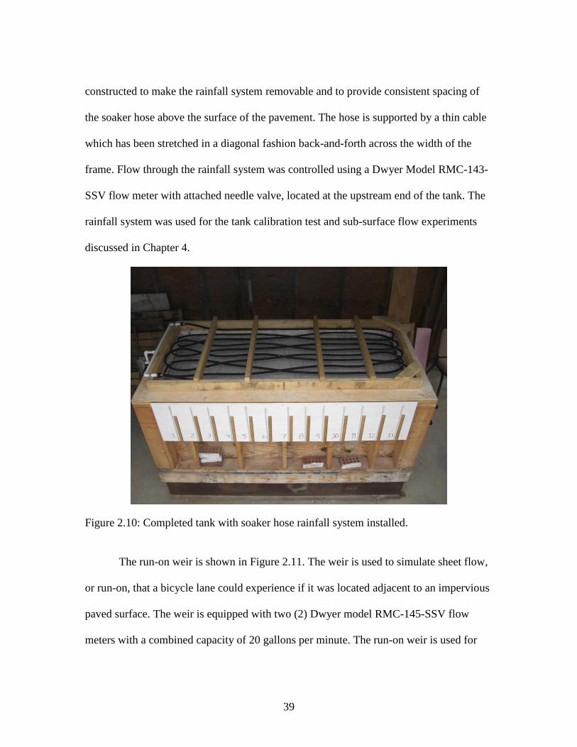
39

constructed to make the rainfall system removable and to provide consistent spacing of

the soaker hose above the surface of the pavement. The hose is supported by a thin cable

which has been stretched in a diagonal fashion back-and-forth across the width of the

frame. Flow through the rainfall system was controlled using a Dwyer Model RMC-143-

SSV flow meter with attached needle valve, located at the upstream end of the tank. The

rainfall system was used for the tank calibration test and sub-surface flow experiments

discussed in Chapter 4.

Figure 2.10: Completed tank with soaker hose rainfall system installed.

The run-on weir is shown in Figure 2.11. The weir is used to simulate sheet flow,

or run-on, that a bicycle lane could experience if it was located adjacent to an impervious

paved surface. The weir is equipped with two (2) Dwyer model RMC-145-SSV flow

meters with a combined capacity of 20 gallons per minute. The run-on weir is used for

40

the surface flow experiments and the sub-surface flow experiments which are discussed

further in Chapters 3 and 4, respectively.

Figure 2.11: Completed run-on weir used for surface flow experiments.

2.4.1.1 Procedure for Surface Flow Experiment

The surface flow experiments were conducted utilizing the bicycle lane test rig

according to the following procedures. To setup the experiment, the weir was placed on

the surface of the pervious pavement at the upstream end of the test rig as seen in Figure

2.11, and also in the diagram of the experimental setup Figure 2.12; a water hose was

connected between a spigot and the flow meter attached to the weir to provide the water

necessary to complete the experiment.

41

Figure 2.12: Surface flow experimental setup.

Before each successive experiment, the upstream end of the test rig was raised or

lowered to maintain the desired pavement slope for that experiment. To begin the

experiment, the spigot was opened on the water supply followed by the needle valve on

the flow meter which was adjusted to the desired flow rate output, beginning with the

minimum flow rate tested for that particular slope. Once satisfied that the flow was

stable, the width of flow, W, (perpendicular to the direction of flow), the maximum length

of flow, Lmax, and the minimum length of flow, Lmin, (measured from the edge of the weir

were recorded as shown in Figure 2.13.

Figure 2.13: Surface flow experiment measurements.

Following the completion of one experiment, the flow rate was increased to the

next highest value and the process was repeated until results had been recorded for each

flow rate at that particular slope. Finally, the slope experiments were repeated for each

slope value completing the series of experiments.

42

2.4.1.2 Procedure for Sub-Surface Flow Experiment

The sub-surface flow experiments were also conducted using the bicycle lane test

rig in a similar fashion as the surface flow experiments with a few additions to the

method. To setup the experiment, the weir was placed on the surface of the pervious

pavement at the upstream end of the test rig as seen in Figure 2.11, and the rainfall

system was situated over top of the weir and bicycle lane test rig. Separate water hoses,

each with its own spigot, were connected to the inlet of the flow meters attached to the

weir and rainfall system to provide the water necessary to complete the experiment and to

allow each system to be regulated independently.

Again, before each successive experiment, the upstream end of the test rig was

raised or lowered and blocked to maintain the desired pavement slope for that

experiment. Once the proper slope was established, the experiment could be conducted.

To begin the experiment, the spigots were opened on the water supplies followed by the

needle valves on the flow meters which were adjusted to the desired flow rate output,

beginning with the minimum flow rate tested for that particular slope. Once satisfied that

the flow was stable, a timer was started. The flow rate meters were periodically inspected

to ensure that the flow rates remained consistent throughout the experiment.

Measurements of the sub-surface flow were recorded by photographing the height

of water inside of the manometer tubes shown in Figure 2.10. After the water level had

sufficiently risen inside of the test rig to maintain pressure in the manometer tubes, the

manometer tubes were purged of air bubbles and a few drops of red food coloring were

placed in each tube to increase the visibility of the water surface. Three photographs were

43

taken at 5 minute intervals, 5, 10, and 15 minutes respectively, from the time the timer

began counting.

Once the series of photographs were complete for each experiment, the

appropriate flow meter was adjusted to begin the next trial. It was considered preferential

to vary the weir flow rate, completing all experiments for one rainfall rate and slope

condition before changing the rainfall rate or slope. The various flow rate combinations

were completed for each slope and weir height.

2.4.2 Falling Head Permeameter

Falling head permeameters are used to measure the hydraulic conductivity of

porous, or pervious, materials. These apparatus were used to determine the hydraulic

conductivity of the No. 57 stone aggregate and the pervious concrete cylinders. Figure

2.14 is a schematic of the permeameters that were constructed for use in these

experiments.

44

Figure 2.14: Schematic diagram of falling head permeameter.

The falling head permeameters were configured to perform a falling head test

with a constant tailwater elevation, ASTM D5856-95 – Test Method B. The main body of

the permeameter was constructed of 150 mm [6 in] schedule 40 clear PVC pipe. Clear

pipe was selected to allow the operator to observe the water level inside of the

permeameter. Next, two PVC reducers, one 150 x 100 mm [6 x 4 in] and one 100 x 50

mm [4 x 2 in], were used to reduce the pipe diameter from 150 mm to 50 mm. A 50 mm

[2 in] PVC ball valve was then attached to the base of the permeameter. The constant

tailwater elevation was maintained using a standpipe constructed of 50 mm [2 in] PVC

pipe which was attached to the valve outlet by a 50 mm [2in] flexible coupling with hose

45

clamps. Two ninety degree PVC elbows were used to reverse the direction of flow up

through the standpipe. Figure 2.15 shows a photograph of the completed permeameter.

Figure 2.15: Falling head permeameter used to determine hydraulic conductivity of

pervious concrete cylinders and No. 57 aggregate.

2.4.2.1 Procedure for Determining Hydraulic Conductivity of Porous Materials

The falling head permeameter was used to determine the hydraulic conductivity

of the No. 57 stone and the pervious concrete specimens. The procedure for the

experiments was consistent; however the sample preparation varied slightly.

The No. 57 stone samples were placed inside the larger standpipe of the

permeameter. A 152 mm [6 in] diameter circular piece of expanded metal was placed into

46

the permeameter before the aggregate to provide an even bottom surface and prevent the

aggregate from entering the reducer segments. Aggregate was placed in the permeameter

to a depth of 152 mm [6 in.] where it was leveled and compacted to match its placement

inside the bicycle lane test rig.

The preparation of the pervious concrete samples was more complex as care must

be taken to ensure that the water flows through the specimen during the experiment rather

than between the specimen and side wall of the permeameter. To accomplish this, the

cylinders were first wrapped around the top with a layer packaging tape which was folded

to allow approximately one-third of its width to contact exterior rim of the cylinder and

the remaining two-thirds to extend above the top of the cylinder facing outward as shown

in Figure 2.16.

Figure 2.16: Pervious concrete cylinder prepared for testing in falling head or forced flow

permeameter.

The outside face of the cylinder was then wrapped with clear plastic wrap making

sure that the plastic overlapped the packaging tape creating a secure seal. Care was taken

to prevent obstructing the top and bottom of the cylinders. The prepared cylinders were

47

then placed inside the permeameter and pushed to the bottom of the standpipe. Plumbers

putty was then spread around the top edge of the packaging tape sealing it to the inside of

the permeameter.

To complete the experiment, the valve was closed and the permeameter was filled

until the water reached a height of 381 mm [15 in] above the sample. The 50 mm [2 in]

standpipe was also filled with water until it overflowed. For each trial, the valve was

opened and the time required for the water level to drop from 305 mm [12 in] to 76 mm

[3 in] was recorded. Three trials were performed for each cylinder and the hydraulic

conductivity was determined from the average of the results.

2.4.3 Forced Flow Permeameter

The forced flow permeameter was designed and constructed to develop a more

precise method of determining the permeability, and thus the hydraulic conductivity of

pervious concrete specimens. The purpose of this device is to measure the permeability of

specimens subjected to a constant flow rate of fluid.

Figure 2.17 is a schematic diagram of the forced flow permeameter. The main

body of the apparatus was constructed entirely of 150 mm [6 in] schedule 40 PVC pipe.

The 150 mm pipe was selected to provide a uniform cross-sectional area for the control

volume surrounding the pervious concrete specimens which were 152 mm [6 in] in

diameter. The specimen chamber was constructed of clear 150 mm [6 in] schedule 40

PVC to allow observation of the test specimen during experimentation and is connected

to the main body of the apparatus by flange connections. Two brass barbs were threaded

into holes drilled into the PVC pipe directly above and below the specimen chamber to

48

allow measurement of the pressure difference across the pervious concrete cylinders. A

manometer was created by attaching clear PVC tubing to these barbs and extending the

tubing to a measurement board suspended above the apparatus as seen in Figure 2.18.

A standpipe was constructed and attached to the outlet side of the apparatus using

50 mm [2 in] schedule 40 PVC in a similar fashion to the standpipe on the rigid wall

permeameters. This prevents air bubbles from entering the area beneath the specimen

maintaining a steady flow along with a measureable pressure gradient. A 50 mm [2 in]

brass ball valve was included to control the outlet of the apparatus. A flow meter was

attached to the inlet side of the apparatus by threading a brass fitting into a 150 mm [6 in]

PVC cap attached to the upstream end of the six-inch PVC section. Finally, two ninety

degree elbows were used to redirect the flow of water being pumped from a 0.2 m3 [55

US Gallon] drum, up through the flow meter, and back down vertically through the

specimen.

49

Figure 2.17: Schematic diagram of forced flow permeameter.

Water used for the experiment was pumped from the plastic drum and circulated

through the testing apparatus using a submersible sump pump which was lowered into the

drum and connected to the flow meter via flexible tubing. Figure 2.18 is a photograph of

the completed forced flow permeameter.

50

Figure 2.18: Forced flow permeameter apparatus.

2.4.3.1 Procedure for Forced Flow Permeability Experiment

The forced flow permeameter was used to determine the permeability and thus the

hydraulic conductivity of the pervious concrete cylinders. Again, special care was taken

while preparing the cylinders for testing to ensure that the water flows through the

specimen during the experiment rather than between the specimen and side wall of the

permeameter. The cylinders were first wrapped around the top with a layer packaging

tape which was folded to allow approximately one-third of its width to contact exterior

51

rim of the cylinder and the remaining two-thirds to extend above the top of the cylinder

facing outward as shown in Figure 2.16. The outside face of the cylinder was then

wrapped with clear plastic wrap making sure that the plastic overlapped the packaging

tape creating a secure seal. Care was taken to prevent obstructing the top or bottom of the

cylinder.

The prepared cylinder was then placed inside the specimen chamber of the

permeameter and pushed down until it rested on the support at the bottom. Plumbers

putty was then spread around the top edge of the packaging tape sealing it to the inside of

the permeameter. The specimen chamber was then securely bolted between the main

body of the permeameter and the valve and standpipe assembly being sealed by the

gaskets inserted between the respective flanges. Finally, the manometer tubes were

attached to the barb ports above and below the specimen chamber to allow for

measurement of the pressure difference across the cylinder.

Before the experiment could begin, the brass ball valve was closed and the

permeameter was filled. The air release valve at the top of the permeameter was opened

as the chamber was filled to allow the air inside of the permeameter to be purged. The 50

mm [2 in] standpipe was also filled with water until it overflowed. Once the permeameter

had been purged of as much air as possible, the experiment was ready to begin.

To begin each trial, the submersible pump was started and the needle valve on the

flow meter was opened while simultaneously opening the brass ball valve allowing both

inflow and outflow. The flow rate was adjusted to 2.5*10-4

m3/s [4.0 GPM] and the flow

was allowed to stabilize. Once the flow was stable, the head difference between the two

52

manometer tubes was measured and recorded. Next, the flow rate was reduced to 2.2*10-4

m3/s [3.5 GPM] and the head difference was again measured. This process was repeated,

reducing the flow rate by 3.2*10-5

m3/s [0.5 GPM] increments until the flow rate was

reduced to 6.3*10-5

m3/s [1.0 GPM]. After taking the final measurement, the pump was

stopped and the system was allowed to drain before removing the cylinder from the

permeameter and repeating the process.

53

CHAPTER THREE

SURFACE FLOW EXPERIMENTS

It is intuitive to begin creating a hydraulic model for a pervious pavement bicycle

lane section where the first interaction with rainfall and runoff occurs, namely at the

pavement surface. If the bicycle lane is to be located alongside an urban street, it can be

used to both intercept the rainfall falling from above and the run-on created by the

adjacent impervious pavement section. This experiment examined multiple flow rates of

runoff and multiple pavement slopes to determine which variable has the greatest

influence on the ability of the pervious pavement to infiltrate the surface runoff and

prevent the ponding of water on its surface.

The objectives of this experiment were: 1) to determine the effects of slope on

surface infiltration rates of pervious pavements, 2) to create a numerical model to use for

the design of porous pavement bicycle lanes along impervious roadways, and 3) to

validate the numerical model for surface infiltration through experimental testing of a full

scale bicycle lane model.

3.1 Model Development

A model, which accounts for both vertical infiltration and lateral flow along the

slope, is necessary to properly characterize the flow of stormwater within the pervious

bicycle lane system. This model must also be able to account for precipitation as well as

run-on from the adjacent impervious surface.

54

Figure 3.1: Schematic diagram of surface flow model.

Two basic equations are needed to model flow in the system: 1) the conservation

of volume or continuity equation and 2) the conservation of momentum equation. The

simplified continuity and momentum equations for a wide rectangular channel are given

in (3.1.1) and (3.1.2) where q denotes the flow rate per unit width along the slope (x-

direction), y denotes the depth of flow in the channel, i is the rainfall intensity, and f is the

infiltration rate.

dq dy

i fdx dt

(3.1.1)

2

0 f

d d q dyq gy gy s s

dt dx y dx (3.1.2)

In the momentum equation (3.1.2), g is the gravitational acceleration constant, s0

is the bed slope, and sf is the friction slope. The friction slope is calculated from the

Manning equation using

2 2

43

f

u ns

R , (3.1.3)

55

where u is the velocity of the water, n is Manning’s roughness coefficient, and R is the

hydraulic radius. The hydraulic radius can be approximated as the depth of water, y, for a

wide rectangular channel, and will be used to approximate the hydraulic radius for the

bicycle lane.

The equations above account for flow occurring on the surface of the bicycle lane

system. In this scenario, sub-surface flow is also occurring and will be discussed further

in Chapter 4.

3.2 Steady State Solution

The first step in the combined flow model was to determine the steady state

surface infiltration rate and the corresponding wave. The goal was to determine the

relationship between hydraulic conductivity, which is determined from the infiltration

rate, and the pavement slope for a constant run-on rate and no rainfall rate. Combining

equations (3.1.2) and (3.1.3) then removing the time dependent and rainfall terms from

equations (3.1.1) and (3.1.2) yields:

dq

fdx

(3.2.1)

2 2

2

0 43

2dy u n

gy u gy s ufdx y

. (3.2.2)

The infiltration rate, f, is approximated by the Green-Ampt model in which the

infiltration rate is the intrinsic permeability multiplied by the head divided by the

thickness of the saturated layer. The depth of the saturated layer is taken to be the

pavement thickness. This assumes that saturated flow occurs in the pavement only and

56

the pressure in the aggregate subbase remains atmospheric which is reasonable given that

the subbase porosity and hydraulic conductivity will be substantially larger than the

pavement. Writing this in terms of the hydraulic conductivity instead of the permeability

yields

1y

f KT

. (3.2.3)

The depth of sheet flow runoff from a paved surface is typically a few

millimeters, and pervious pavements are typically placed with a depth between 50 and

150 millimeters to provide structural resiliency. It can be seen that the infiltration rate

function, f, can be further simplified when the depth, y, is much smaller than the

pavement thickness, T, yielding

f K . (3.2.4)

Furthermore, as the ratio of depth to pavement thickness increases, the infiltration rate

function, f, also increases. Therefore, the approximation (3.2.4) provides a conservative

estimate of the infiltration rate and the conservation of volume becomes,

dq

Kdx

. (3.2.5)

This can be integrated from the initial flow rate per unit width q=q0 at x=0 to q=0 to

establish the distance xmax taken for the run-on to fully infiltrate,

0max

qx

K . (3.2.6)

This can be easily extended to the case of constant rainfall intensity, i, by adding the

rainfall intensity to the right hand side of (3.2.5). In this case (3.2.6) becomes,

57

0max

qx

K i

(3.2.7)

Provided the rainfall intensity is considerably less than the hydraulic conductivity of the

pavement, the correction for rainfall will make a negligible difference to the run-on

distance. This is not an onerous constraint as typical pavement hydraulic conductivities

are several orders of magnitude larger than even 100 year storm rainfall intensities. The

results presented in (3.2.7) means that, to first order, the distance to full infiltration of the

run-on can be calculated without having to solve the momentum equation.

3.3 Surface Flow Experiments

The infiltration rate of the pervious concrete slab cast inside of the bicycle lane

test rig was determined at three representative locations using ASTM C 1701 Standard

Test Method for Infiltration Rate of In-Place Pervious Concrete. The results of these tests

are listed in Table 3.1 and are used to determine the intrinsic permeability and hydraulic

conductivity of the pavement.

Table 3.1: Infiltration rates determined by ASTM C 1701.

Location Infiltration Rate

mm/hr [in/hr]

1 40000 [1580]

2 25600 [1010]

3 25100 [ 990]

Next, a series of tests were performed to determine the behavior of water flowing

as sheet flow onto the surface of a pervious pavement. This would be comparable to

runoff flowing to a gutter from the impervious pavement surface. For the remainder of

this section, this simulated runoff will be referred to as run-on. Utilizing the weir, shown

58

in Figure 3.2, a fixed volume flow rate of water was evenly released across the width of

the pavement at the upstream end. The run-on distance, or the distance from the

downstream edge of the weir spillway to the point where the flow had fully infiltrated,

was measured and recorded for each flow rate and pavement slope combination.

Figure 3.2: Plexiglas weir used to simulate sheet flow across the pervious pavement

surface.

In total, fifteen trials were performed to determine the run-on distance for initial

flow rates of 2.5, 3.8, 5.0, 6.3, and 7.6*10-4

m3/s on pavement slopes equal to 0%, 5%,

and 10%. These values were chosen to represent values of rainfall and slope which could

occur on streets in an urban environment, as well as to capture the extreme events that

may occur due to excessive rainfall intensity or steep slope conditions.

59

Table 3.2: Equivalent surface run-on flow rates.

Metered Flow Rate

[GPM]

Equivalent Flow Rates Flow Rate Per Unit Width

m3/s *10

-4 [ ft

3/s *10

-2] m

3/s /m *10

-4 [ft

3/s/ft *10

-3]

4.0 2.5 [ 0.9 ] 2.8 [ 3.0 ]

6.0 3.8 [ 1.3 ] 4.2 [ 4.5 ]

8.0 5.0 [ 1.8 ] 5.6 [ 6.0 ]

10.0 6.3 [ 2.2 ] 7.0 [ 7.5 ]

12.0 7.8 [ 2.7 ] 7.6 [ 9.0 ]

Flow across the pervious pavement was non-uniform; therefore, the approximate

maximum and minimum flow lengths were recorded for each trial. The range of

measured flow lengths were then plotted and compared with the lengths required for

complete infiltration predicted by the surface flow model, equation (3.2.6), as shown

below in Figure 3.3.

3.4 Surface Flow Experiment Results

Solving the system of differential equations requires an estimate of the hydraulic

conductivity of the pervious pavement that is being modeled. An anticipated value of

hydraulic conductivity could be used for design purposes; however, it was necessary to

determine the in-place hydraulic conductivity of the pervious pavement cast inside the

tank to properly compare the numerical results with the experimentally determined

values. The intrinsic permeability and hydraulic conductivity were calculated from the

infiltration rates determined according to ASTM C 1701 yielding the results listed in

Table 3.3.

60

Table 3.3: Intrinsic Permeability and Hydraulic Conductivity for equivalent infiltration

rates determined in accordance with ASTM C1701.

Infiltration

Rate

Intrinsic Permeability, k

Reynolds

Number Hydraulic Conductivity, K

mm/hr [in/hr] *10-10

m2 [*10

-9 ft

2] m/s [ft/s]

25120 [ 989] 6.399 [ 6.888 ] 0.181 0.0064 [0.0211]

25645 [1010] 6.533 [ 7.032 ] 0.186 0.0066 [0.0216]

40024 [1576] 10.20 [ 10.98 ] 0.363 0.0103 [0.0337]

The intrinsic permeability, k, is found using

I T

kH

(3.3.1)

where I is the infiltration rate obtained by performing ASTM C 1701, µ is the dynamic

viscosity of water, γ is the unit weight of water, T is the thickness of the pavement, and H

is the hydraulic head which equals T plus 13 mm [1/2 in] for tests performed in

accordance with this standard. Next, the Reynolds number, Re, must be calculated using

e

I kR

(3.3.2)

where ν is the kinematic viscosity of water, to ensure that the flow downward through the

pervious concrete follows Darcy’s Law. Finally, the hydraulic conductivity, K, is

determined using

k

K

(3.3.3)

The maximum Reynolds number of 0.363 confirms that the downward vertical

flow occurs within the Darcy flow regime and thus the Forchheimer term can be ignored

in the model (Nield and Bejan 2006). Consequently, each of the hydraulic conductivity

values can be used to solve the set of differential equations without modification.

61

The experimental results obtained from the surface flow test were compared with

the predicted values obtained using equation (3.2.6). Results are reported for the initial

flow rates, q0, ranging from 2.8*10-4

to 7.6*10-4

m2/s gallons per minute and pavement

slopes of 0%, 5%, and 10%. The experimental data is plotted in Figure 3.3 as a bar

extending from the minimum to maximum flow distance with a bar representing the

average. Also shown in Figure 3.3, are the results of the numerical model where the solid

lines represent the lower limit of hydraulic conductivity and the dashed lines represent

the upper limit of hydraulic conductivity. For both hydraulic conductivities, the

approximate solution (3.2.6) and the results of a full numerical solution of (3.2.1) and

(3.2.2) are shown by the solid and dashed lines indicating that (3.2.6) provides an

excellent approximation of the full solution.

62

Figure 3.3: Plot of measured infiltration distance versus flow rate per unit width, q0, for

pavement slopes of 0% (blue), 5% (red), and 10% (green). The same five flow rates were

tested for each slope; however, q0 varies due to flow width contraction. The solid line

represents model results for hydraulic conductivity, K, equal to 0.0064 m/s, and the

dashed line represents K equal to 0.0103 m/s.

3.5 Discussion and Conclusions

The results of the numerical model for the surface flow test indicate that the

distance required for infiltration of surface run-on, or sheet flow that flows across the

pervious pavement surface increases as the flow rate increases. Infiltration appears to be

most affected by the distribution of pore spaces in the pervious concrete surface. Also,

the average distance required for infiltration for all experimental observations lie beneath

the model output for both the minimum and maximum hydraulic conductivity of the

63

pavement slab. Therefore, it is reasonable to conclude that using the minimum hydraulic

conductivity to estimate the maximum distance required for complete infiltration will

result in a conservative estimate of the run-on distance. Finally, the experimental results

yield a maximum run-on distance of approximately 0.13 m [5.12 in] for a run-on rate per

unit width equivalent to that from one 3.66 m [12 ft] width impervious lane, with a 1%

cross slope and a 5% longitudinal slope for a rainfall intensity of 224 mm/hr [8.83 in/hr].

A comparison of the numerical model and the results of the surface run-on test

indicate that the St. Venant equations can be used to reasonably predict the maximum

distance required for complete infiltration of runoff. However, it should also be noted

that the solution can be further simplified when the depth of flow is much smaller than

the thickness of the pavement, which is generally the case. Therefore, the maximum run-

on distance is equal to the ratio of the flow rate per unit width and the hydraulic

conductivity as seen in (3.2.6).

The results of this experiment provide the engineer with a method of determining

the required hydraulic conductivity and lane width necessary to infiltrate both the rainfall

falling directly on the pervious surface of the bicycle lane and the run-on produced by the

adjacent impermeable area. Figure 3.4 is a simplified typical cross-section of a pervious

bicycle lane located adjacent to an impervious traffic lane. The traffic lane has a width,

wL, and a hydraulic conductivity, K, which is approximately zero. Similarly, the bicycle

lane has a width, wB, with a hydraulic conductivity, Kreq, which is the design target of

hydraulic conductivity for the pervious pavement. The rainfall intensity, i, is obtained

from local weather data and the codified design storm event.

64

Figure 3.4: Pervious bicycle lane design section.

Rearranging, (3.2.6) with the conditions that

max Bx w (3.4.1)

and

0 L Bq i w w (3.4.2)

the equation for the required hydraulic conductivity becomes

L Breq

B

w wK i

w

. (3.4.3)

This simplification can be made as the peak flow rate does not depend on the slope

directly, but rather the contributing area and the time of concentration of that area, which

is often small and taken as 5 minutes rather than the calculated time, unless the calculated

time is larger than 5 minutes. Equation (3.4.3) can also be rearranged to determine the

65

required pervious bicycle lane width when the hydraulic conductivity of the pervious

pavement is known or dictated by in-situ conditions or material properties yielding

,L

B req

iww

K i

. (3.4.4)

In summary, the numerical surface flow model has been shown to accurately

predict the maximum infiltration distance within the range of experimental values when

computed using the maximum hydraulic conductivity obtained from the results of the in-

place infiltration test ASTM C 1701. Further modeling and experimental verification is

required to determine if ponding would occur on a bicycle lane surface as the run-on flow

rate increases due to the addition of impervious surface or increased rainfall, or if the

potential for ponding increases as the hydraulic conductivity decreases due to surface

clogging or other factors.

3.6 Surface Design Procedure

The following procedure can be used to determine the required bicycle lane width

and hydraulic conductivity to intercept a design storm event without ponding. Note that

the following equations consider only rainfall falling on the paved surface as shown in

the simplified diagram of Figure 3.4; however, with proper adjustment for the initial flow

rate, the procedure remains applicable.

1. Determine the maximum allowable run-on distance. For simplicity, the

maximum allowable run-on distance can be taken as the width of the bicycle

lane (3.4.1), or as the width of the pervious pavement area.

66

2. Determine the required hydraulic conductivity, Kreq, using (3.4.3) given the

initial flow rate per unit width (3.4.2), or

3. Determine the required pervious lane width, wB, using (3.4.4) given the

hydraulic conductivity of the pervious pavement, K, the rainfall intensity, i,

and the width of impervious areas, wL.

67

CHAPTER FOUR

SUB-SURFACE FLOW EXPERIMENTS

Continuing on from the results of the surface flow model in the previous chapter,

it is prudent to next account for the flow of water as it enters and flows through the

aggregate base layer beneath the pervious concrete slab. Figure 4.1 is an extension of

Figure 3.1 showing the sub-surface flow characteristics. It can be seen that as the rainfall,

i, and the run-on, Qin, infiltrate through the pervious concrete, fconc, a number of different

things can occur with this infiltrated water.

Figure 4.1: Schematic diagram of sub-surface flow model.

First, the water could continue to infiltrate into the underlying native soil beneath

the bicycle lane, fsoil. Second, if the combined volume of the rainfall and run-on exceeds

the infiltration capacity of the native soil, the water can begin to accumulate in the

aggregate base layer as noted by the dashed arc in Figure 4.1. Finally, if the plane

separating the native soil and the aggregate layer is located on a slope, water may flow

68

laterally, downslope, resulting in a discharge Qout, through the aggregate layer to a low-

point in elevation where it will accumulate.

As noted in the literature, infiltration practices are often limited by the ability of

the native soil to infiltrate water. These practices are often sized by balancing the depth of

aggregate necessary to provide a storage volume capable of storing the runoff until it is

able to infiltrate into the underlying native soil. Sizing the storage volume requirements

for pervious pavements on level ground is easily accomplished; however, the situation

becomes more complex on sloping terrain and the storage capacity of the aggregate layer

becomes greatly reduced.

Instead of the water level rising evenly in the aggregate base as it would on a level

or nearly level site, the water in a system with a sloped surface, see Figure 1.1 (a) will

flow to and accumulate at sag locations, or low-points, along the alignment of the

roadway. If the volume of water that accumulates at the sag point of the roadway exceeds

the storage capacity at that location, the water will rise above the surface of the pavement

creating a ponded water condition. This ponded water condition could cause both the

bicycle lane and the adjacent roadway to become unusable; something that would be

unacceptable to local and state transportation departments.

Several potential solutions have been proposed to prevent this ponded condition

from occurring and maintain the viability of the application of pervious pavements along

sloped areas. Two prominent ideas are to install weirs at regular intervals, as necessary,

along the length of the bicycle lane and to stair-step the native soil beneath the base

material to provide additional storage and flat areas to promote the vertical infiltration of

69

water into the soil, see Figure 1.1 (b), (c), and (d). Additionally, underdrains could be

installed to remove the excess water and transfer it to a traditional storm drainage system

for extreme storm events.

This experiment examined multiple combinations of rainfall and run-on flow rates

for multiple pavement slopes with various outlet conditions to determine the flow

regimes within the aggregate base material. The objectives of this experiment were: 1) to

determine the effects of slope on the sub-surface flow of runoff through the aggregate

base material, 2) to create a numerical model to use for the design of the base material

section of the porous pavement bicycle lane, and 3) to validate the numerical model for

sub-surface flow through experimental testing of a full scale bicycle lane model.

4.1 Model Development

The continuity equation (4.1.1) still holds though it must be adapted to account

for the presence of the porous media. A diagram of the situation is shown in Figure 4.2.

0out in

dVQ Q

dx (4.1.1)

70

Figure 4.2: Aggregate base layer control volume.

Considering a control volume of length dx and transverse width w we can write

(4.1.1) as

0o s

dwydx u du yw uyw f wdx f wdx

dt . (4.1.2)

Simplifying and dividing by dx yields the final modified continuity equation

0s

dq dyf f

dx dt . (4.1.3)

Darcy’s law,

k dP

udx

, (4.1.4)

71

gives the velocity of a fluid through a porous media for pressurized flow. The velocity is

a function of the permeability, k, of the porous media, the viscosity, μ, of the fluid, and

the pressure gradient.

According to Dupuit (1863) and Forchheimer (1901), an additional term needs to

be added to Darcy’s law to account for the non-linearity of the velocity term.

1

2 2

F f

dP ku c k u

dx

(4.1.5)

For the Forchheimer equation, k is the permeability of the porous media, cF is the form-

drag constant, and ρf is the fluid density. Re-writing equation (4.1.5) for non-pressurized

flow yields

12 2

2

Fag

q c k qs

kg y g y

(4.1.6)

this is written in a form equivalent to the friction slope due to bed shear stress and

represents the increased friction slope due to the presence of the porous material in the

channel section. In equation (4.1.6), ν is the kinematic viscosity of the fluid, q is the flow

rate per unit width, y is the depth of the fluid, and g is the gravitational acceleration

constant.

Several studies have been undertaken to determine the solution for the form drag

constant, cF, including Ward (1964), Beavers et. al. (1973), Coulaud et. al. (1988), and

Kaviany (1995) among others. Ward (1964) believed that the value cF might be a

universal constant 0.55; however Beavers et. al. (1973) determined that effects from the

boundaries could reduce the factor cF according to

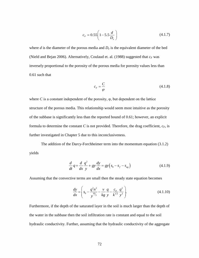
72

0.55 1 5.5F

e

dc

D

(4.1.7)

where d is the diameter of the porous media and De is the equivalent diameter of the bed

(Nield and Bejan 2006). Alternatively, Coulaud et. al. (1988) suggested that cF was

inversely proportional to the porosity of the porous media for porosity values less than

0.61 such that

F

Cc

(4.1.8)

where C is a constant independent of the porosity, φ, but dependent on the lattice

structure of the porous media. This relationship would seem most intuitive as the porosity

of the subbase is significantly less than the reported bound of 0.61; however, an explicit

formula to determine the constant C is not provided. Therefore, the drag coefficient, cF, is

further investigated in Chapter 5 due to this inconclusiveness.

The addition of the Darcy-Forchheimer term into the momentum equation (3.1.2)

yields

2

0 f ag

d d q dyq gy gy s s s

dt dx y dx (4.1.9)

Assuming that the convective terms are small then the steady state equation becomes

2 2 2

0 10 1 2 23

Fdy q n v q c qs

dx kg y k yy

. (4.1.10)

Furthermore, if the depth of the saturated layer in the soil is much larger than the depth of

the water in the subbase then the soil infiltration rate is constant and equal to the soil

hydraulic conductivity. Further, assuming that the hydraulic conductivity of the aggregate

73

and pavement is large compared to the rainfall intensity and that there is no significant

storage and lag time for the vertical flow down to the base of the aggregate then

continuity becomes

L B

soil

B

w wdqi K

dx w. (4.1.11)

The system of ODE’s (4.1.10) and (4.1.11) in y and q can be solved numerically given

appropriate boundary conditions and information about the rainfall rate, aggregate

permeability, and soil permeability. However, for most realistic cases, the soil

permeability often controls design as it can be orders of magnitude smaller than the

permeability of the pervious pavement and aggregate subbase. This fact yields that

utilizing a uniform depth section of pervious pavement and aggregate subbase, Figure 1.1

(a), would be impractical on long slopes.

Therefore, two options exist if using a pervious pavement system is desired. First,

the subgrade beneath the pervious pavement section could be leveled as seen in Figure

1.1 (c) and (d), s0=0.00, which is the case often seen where pervious pavements are

utilized in parking lots. Second, weirs constructed of an impermeable material could be

placed perpendicular to the slope at specified locations to create reservoir areas capable

of storing the necessary rainfall and runoff until it can be infiltrated by the native soil as

seen in Figure 1.1 (b) and (d).

In either case, the depth of flow will be large compared to the aggregate size, the

flow rate per unit width will be small, and the water surface will be approximately

74

horizontal. Therefore, the momentum terms can be ignored and the focus switched to the

weir flow.

The discharge, Q, from a reservoir controlled by a sharp crested, rectangular weir

can be calculated by

3 22

23

dQ C gLH (4.1.12)

where, Cd is the weir discharge coefficient,

0.602 0.075d

HC

P (4.1.13)

L is the distance across the weir, g is the gravitational acceleration constant, H is the

depth of water above the crest of the weir, and P is the weir height (Gupta 2008). This

equation assumes that the entire length of the weir is unobstructed and water is allowed to

flow freely across its surface. However, when the weir is placed within the aggregate

subbase layer, the length of the weir should be reduced to account for the portion which

is obstructed by individual aggregate particles along its length. This is especially

important when the depth of water over the weir, H, is less than or approximately equal to

the nominal maximum size of the aggregates in the subbase, as is the case for the bicycle

lane. Therefore, an appropriate scaling factor must be selected to account for this

reduction in the effective length of the weir. Intuition yields that the effective weir length

would be proportional to the porosity, φ, or void content of the aggregate subbase.

Therefore, the right hand side of (4.1.12) is multiplied by the porosity, φ, yielding

3

22

23

dQ C L gH (4.1.14)

75

Designing the bicycle lane as a series of reservoirs with rectangular weir outlets

transforms the design situation from an open channel problem to a reservoir routing

problem where the subbase depth, weir height, and weir locations can be designed based

on storage and drawdown requirements.

4.2 Test Rig Calibration

Before conducting the sub-surface flow experiments, the test rig was calibrated to

account for any leaks or other minor losses that would affect the correlation between

experimental results and predicted outcomes. The top of the soil layer was sealed with a

sheet of plastic to simulate a zero infiltration condition for the experiments conducted in

this study. The results of the calibration tests were used to verify the numerical model and

to examine the storage capacity of the aggregate base layer.

The test rig was calibrated by leveling the frame and sealing the open end of the

test rig with Styrofoam as shown in Figure 2.11. Three constant rainfall intensities, listed

in

Table 4.1, were simulated using the soaker hose, and the depth of water in the

aggregate layer was recorded at constant time intervals as the tank was filled. Figure 4.3

depicts a calibration test in progress. The water surface level inside the tank was

indicated by the level of the water, enhanced with red food coloring, in the manometer

tubes located along the side of the tank.

Table 4.1: Simulated rainfall intensities for calibration tests.

Metered Flow Rate [GPM] Equivalent Rainfall Intensity

mm/hr [in/hr]

76

0.4 47 [ 1.9]

1.0 118 [ 4.6]

2.5 295 [11.6]

Figure 4.3: Image of calibration testing. Red food coloring was used to enhance the

resolution of the water level inside manometer tubes. Photos were taken at regular

intervals to determine the change in depth of water within the aggregate layer over time.

Assuming the tank is free of leaks, a plot of depth versus time will give a straight

line of slope equal to the filling rate (dh/dt) which can be related to the imposed rainfall

rate (i) and the layer porosity (φ) by

dh i

dt . (4.2.1)

This relationship must be modified due to the existence of an air void space located at the

open end of the test rig, between the aggregate and concrete and the foam used to seal the

tank, yielding equation (4.2.2) where Apave is the area of the pavement and Avoid is the area

of the void.

pave

pave void

iAdh

dt A A

(4.2.2)

77

4.2.1 Calibration Test Results

The porosity, or void content, φ, was used to determine the storage capacity of the

aggregate layer. The calibration test was performed a total of five times, and the data are

plotted in Figure 4.4. The slope was determined for the straight line portion of each

filling curve, and the respective porosity values were calculated using (4.2.2). The results

are listed in Table 4.2.

Table 4.2: Calibration test results.

Test Number Rainfall Rate

Slope (dh/dt) Porosity (φ) m

3/s *10

-5 [GPM]

1 15.8 [ 2.5 ] 0.009587 0.32

2 15.8 [ 2.5 ] 0.009441 0.32

3 6.3 [ 1.0 ] 0.003933 0.31

4 2.5 [ 0.4 ] 0.001949 0.25

5 2.5 [ 0.4 ] 0.002058 0.23

78

Figure 4.4: Plots of water surface elevation (y) versus elapsed time for each of five

calibration tests.

79

The results of the calibration test listed in Table 4.2 indicate that the measured

porosity varies with the imposed rainfall rate. The lower the rainfall rate, the lower the

measured porosity. This indicates that there is some leakage from the tank or infiltration

through the plastic membrane separating the aggregate from the underlying soil.

Therefore, an additional term for the leakage rate, L, must be subtracted from the right

hand side of equation (4.2.2) yielding,

pave

pave void

iAdhL

dt A A

(4.2.3)

The porosity of the aggregate within the tank is then approximated by testing

various values of φ to find the value that minimizes the standard deviation of the leakage

rate across all tests. This analysis yields an estimated porosity of φ= 0.34. The resulting

estimated leak rate was 9.2*10-6

m3/s [3.3*10

-4 ft

3/s]. Additionally, the porosity, or void

content, of a sample of the aggregate base was determined in accordance with ASTM C

29 and found to be 0.36. The estimated porosity, φ, of 0.34 would appear reasonable

since there is no precision data provided in ASTM C 29 for void content and the fact that

void content is dependent on many factors including aggregate shape and level of

compaction.

4.3 Sub-Surface Flow Experiments

A series of sub-surface flow experiments were conducted using the bicycle lane

test rig to characterize the sub-surface flow regimes of water within the aggregate layer

for various flow, slope, and outlet conditions. As noted previously, the soil type and level

of compaction among other factors can greatly affect the ability of a soil to infiltrate

80

water and prevent the accumulation of water within the aggregate layer. Due to the high

degree of variability of soil infiltration rates, this study was limited to observe the

behavior of the fluid flow for the case where zero infiltration occurs into the underlying

native soil. Therefore, all sub-surface flow experiments were completed with the plastic

membrane placed between the soil and aggregate layers in the test rig, as in Figure 2.7,

simulating a zero infiltration condition.

Experiments were conducted for multiple combinations of the rainfall and run-on

flow rates listed in Table 4.3 with the test rig inclined at two (2), four (4), and six(6)

percent and the outlet controlled by either a 38 mm [1.5 in.], 76 mm [3 in], or 114 mm

[4.5 in.] tall weir as shown in Figure 4.5. The duration of each experiment was fifteen

(15) minutes, and photographs of the manometer panel were taken every five (5) minutes

to record the water surface level inside of the aggregate layer. The water surface level in

the manometer tubes was measured on the photographs and recorded in a spreadsheet.

Table 4.3: Metered flow equivalents for sub-surface flow test.

Rainfall [GPM] Equivalent Rainfall Intensity

mm/hr [in/hr]

1.5 177 [ 7.0]

2.0 236 [ 9.3]

2.5 295 [11.6]

Run-on [GPM] Equivalent Run-on Rate

*10-5

m3/s [*10

-3 ft

3/s]

1.0 6.3 [ 2.2]

2.0 12.6 [ 4.5]

3.0 18.9 [ 6.7]

5.0 31.5 [11.1]

7.0 44.2 [15.6]

81

Figure 4.5: Outlet control weir at downstream outlet of bicycle lane test rig.

Photographs for these experiments were taken with a Panasonic Lumix DMC-TS4

12.1 megapixel digital camera. The resolution of the photographs was sufficient to record

measurements to the nearest 1.6 mm [0.625 in.] when the photographs were enlarged in

Microsoft Picture Viewer. Approximately 2 mL of red food coloring was injected into

each manometer tube to enhance the visibility of the water surface level inside of the

tube. Figure 4.6 shows an example image from one of the sub-surface flow experiments.

82

Figure 4.6: Sub-surface flow test image for experiment with slope=0.02, i = 295 mm/hr

[2.5 GPM], Q = 18.9*10-5

m3/s [3.0 GPM], and weir height = 114 mm [4.5 in.]

4.4 Sub-Surface Flow Experimental Results

A total of 148 unique sub-surface flow experiments were conducted over the

duration of this project. Figure 4.7 shows a plot which is typical of the results for each

sub-surface test. The data plotted in Figure 4.7 is that obtained from the photograph of

the test shown in Figure 4.6.

Each photograph yielded 13 measurements of the depth of water inside the test

rig; however, the depth of water at the weir was not recorded. It is necessary to determine

the depth of water above the weir to determine the discharge using (4.1.14). Linear

extrapolation was used to determine the depth above the weir, H, based on the water

surface elevation of the preceding six measurements. Of the 444 observations calculated,

three for each experiment, 63 of the extrapolations indicated that the water surface

83

elevation at the weir was equal to or below the weir elevation ± 1.6 mm, though water

continued to flow over the weir for the duration of each experiment. Therefore, the

surface elevation at the manometer 15.2 cm upstream of the weir was used as an alternate

estimate of the head above the weir. Of these values 400 were above the weir height ± 1.6

mm. The maximum observed difference in the water surface elevation and the weir

elevation for all experiments was 5.8 mm [0.23 in.].

Figure 4.7: Plot of measured results of experiment shown in Figure 4.6. Datum, z=0 is

assumed to be the bed elevation at the base of the weir. Boxes indicate the actual

measured data points.

Figure 4.8 shows the relationship between the head, H, above the weir (the

difference in water surface elevation and weir elevation), and the total flow rate, Qt (the

sum of rainfall and run-on) for each of the 381 calculated H values greater than 0.0 ± 1.6

84

mm. The calculated head values, H, at the weir are plotted as squares and the head, H, at

the first manometer, six inches upstream of the weir are plotted as diamonds. The solid

line plotted in Figure 4.8 is the solution of the weir discharge equation (4.1.14).

Figure 4.8: Plot of Total Flow Rate (Qt) versus H for all sub-surface flow experiment

observations with water surface elevation greater than weir elevation. H at the weir

plotted as squares and H 152 mm [6 in] upstream plotted as diamonds. The solid line

represents the solution to the theoretical sharp crested, rectangular weir equation (4.1.14)

adjusted for the aggregate porosity and the dashed line represents the solution of the

standard rectangular weir discharge equation (4.1.12).

These results seem reasonable given the resolution of the measurements, ± 1.6

mm, and the variability of the input flow rate. The flow rate meters for the rainfall system

and run-on are discretized by 1.26*10-5 m3/s [0.2 GPM] and 6.3*10-6 m

3/s [0.1 GPM]

respectively. Also, the manometer tubes provide an additional source of error as air

85

bubbles often form inside of the tubes and provide inaccurate measurements. Overall, the

modified weir discharge equation appears to reasonably predict the maximum height

above the weir, as only 2.7% of the extrapolated head values at the weir exceed those

predicted using (4.1.12).

4.5 Discussion and Conclusions

Given that the head, H, is small compared to the weir elevation, it is reasonable to

assume that the system can be modeled as a lake problem with a rectangular weir outlet.

Therefore, the momentum is assumed to be zero and the solution reduces to a reservoir

routing situation. Figure 4.9 shows a schematic of the bicycle lane subbase. The objective

is to model the bicycle lane as a series of individual reservoir cells balancing the

dimensions of each cell and outlet controls to provide sufficient retention as the existing

topography allows while ensuring that local drawdown time requirement are met.

Figure 4.9: Pervious bicycle lane subbase reservoir routing diagram.

86

As noted in section 4.1, the weir discharge equation (4.1.12) can be reasonably

modified and scaled by the aggregate porosity, φ, yielding (4.1.14). Inspection of Figure

4.8 indicates that the modified weir discharge equation (4.1.14) provides a reasonably

conservative estimate of the head, H, for a given flow rate, Q.

Therefore, to design the bicycle lane subbase, the designer should first determine

the maximum allowable weir height to meet the drawdown time requirements imposed by

local regulatory agencies. Assuming the section has a level bottom, the drawdown time,

Td, is given by

d

hT

f (4.5.1)

where φ is the porosity of the subbase or aggregate, h is the depth, or stage, of the water

in the subbase; the product φh times the area of the cell is equal to the volume of fluid

retained in the cell for a cell with a horizontal base. This volume will be further reduced

if the base of the cell is sloping. For the denominator, the exfiltration rate is given by the

product φf where f is the constant infiltration rate of the native soil and φ represents the

fraction of the surface area masked by the aggregate particles. If necessary, the

exfiltration rate could be increased by the addition of underdrains; however, the

application of underdrains is beyond the scope of this project.

Next, the base area of each cell is equal to the product of the bicycle lane width,

wB, and the cell length, L. There is no explicit solution for determining the cell length, L.

The design will be restricted by the topography and the vertical profile of the roadway; in

general, the cell length, L, should increase as the pavement slope decreases. In addition,

87

the cell length may be limited by a maximum cut depth or a high water table in the area

of the bicycle lane. Costs may also be a limiting factor as large excavations would require

a large volume of aggregate fill, thereby reducing the maximum volume of the subbase.

Once the allowable geometries of each cell have been determined, the design

storm event should be routed through the bicycle lane’s system of reservoirs to determine

the maximum head, H above the weir for each weir in the system. Figure 4.10 is a cross

section of one individual subbase cell with all of the relevant dimensions labeled.

The stage-storage relationship of an individual cell is given by

BS h Lw h (4.5.2)

where L is the length of the cell and wB is the width of the bicycle lane. Additionally,

Figure 4.10: Schematic diagram of single bicycle lane subbase reservoir cell.

88

The stage-storage relationship of an individual cell is given by

BS h Lw h (4.5.3)

where L is the length of the cell and wB is the width of the bicycle lane. Additionally,

the volume of water stored, S, within the cell varies with time, t, based on the relationship

1 , ,j j B j L j j

dSQ L w i f iw Q

dt (4.5.4)

where the inflow is given by Qj-1, the outflow from the preceding reservoir cell and the

contribution from rainfall is obtained based on the length of the cell, Lj, the width of the

pavement adjacent to the cell, wL,j, the width of the cell, wB,j. The outflow is computed as

the combination of the infiltration rate, φf, and the weir discharge

3 22 23j d BQ C w gH (4.5.5)

The infiltration rate is scaled by the factor φ since the flow is only allowed through that

portion of the soil not covered by solid rock particles (Schwartz 2010).

Finally, some measure of freeboard should be included between the weir elevation

and bottom of the pavement surface to ensure that the water surface elevation remains

within the subbase layer throughout the bicycle lane system. Thus, the minimum depth of

aggregate at the weir is given by

mindepth P H freeboard (4.5.6)

Additionally, the pervious pavement would provide an additional factor of safety to

ponding due to its porous nature.

89

4.6 Sub-Surface Design Procedure

The following procedure can be used to design a pervious bicycle lane subgrade

to control the runoff from a design storm promoting infiltration and meeting drawdown

time requirements of local standards while preventing the ponding of water at sag

locations of the vertical alignment.

1. Determine weir height base on drawdown time using (4.5.1).

2. Determine the length of each cell based on some criteria, possibly:

a) Existing topographic restrictions

b) A prescribed maximum depth of cut based on water table elevation or

reach of excavator

c) Excessive cost associated with the volume of aggregate fill required

3. Route the design storm through the series of reservoirs and determine the

maximum head for each cell using (4.5.4) and (4.5.5).

4. Add weir height, head, and freeboard to determine minimum depth of aggregate

for each cell using (4.5.6).

5. Iterate this design procedure until a desirable and economical solution is found.

90

CHAPTER FIVE

PERMEABILITY EXPERIMENTS

As discussed in Chapter 4, there is some uncertainty in determining the

permeability and thus the hydraulic conductivity of the materials used to construct a

pervious pavement system. These properties become extremely important in situations

where the lateral flow due to gravity driven flow needs to be analyzed.

Classic techniques for measuring the permeability of a course aggregate use a

falling head test method to determine the hydraulic conductivity and then convert the

result to permeability. These test procedures assume that the flow behaves according to

Darcy’s law which is valid only for laminar flow with low Reynolds numbers. However,

experimental results have indicated that these assumptions may be incorrect for higher

Reynolds numbers which occur when the head above the test specimen is large.

Therefore, an alternate method utilizing forced flow permeameter is described here.

5.1 Permeameter Theory

Darcy’s law is given as,

A P

Q kL

(5.1.1)

where Q is the flow rate of the fluid, A is cross-sectional area of the specimen

perpendicular to the direction of flow, ∆P is the change in pressure across the specimen,

L is the length of the specimen, k is the permeability, and μ is the dynamic viscosity of

the fluid. Darcy’s law is valid only when the flow is laminar. Permeability is a measure of

the ability of a pervious material to pass water through its structure and has units of

91

length squared. However, engineers often rely on a related property, the hydraulic

conductivity, K, which has units of length per time in stormwater applications as these

units are easily related to the rainfall rate, which also has units of length per time.

The falling head permeameter test yields the hydraulic conductivity, K, using

relationship

1

2

lnaL h

KAt h

(5.1.2)

where a is the cross-sectional area of the standpipe that the cylinder is inserted into, and t

is the time required for the water to drop from h1 to h2 the initial and final elevations of

water respectively, when using ASTM D5856-95 – Test Method B. Again, this

relationship assumes that flow occurs according to Darcy’s Law and that Reynolds

number is small.

To compare the results of the falling head and the forced flow permeameter test,

the hydraulic conductivity, K, values obtained from the falling head permeameter were

converted to permeability, k, using the relationship

k Kg

(5.1.3)

where ν is the kinematic viscosity of the fluid, and g is the gravitational acceleration

constant. Also, the average Reynolds number is given by

,e Avg

u kR

(5.1.4)

where u is the average velocity given by,

92

Q

uA

. (5.1.5)

However, this approach underestimates the Reynolds number for significant portions of

the experiment as the Reynolds number at any given time is dependent on the ratio of the

head, H, to the length of the specimen, L. The maximum Reynolds number is given by

32

, 2

Maxe Max

H gkR

L . (5.1.6)

The forced flow permeameter yields the head difference, ∆h, for an imposed

velocity of flow, u. The permeability is then obtained by fitting a quadratic function

2hAu Bu

L

(5.1.7)

through the data; ∆h/L and u for the series of flow rates tested and the origin. The

coefficients A and B obtained from the quadratic polynomial can then be used to calculate

two estimates of the permeability, k, where

F

A

cA

g k (5.1.8)

and

B

Bk g

(5.1.9)

according to the general formula of the Darcy-Forchheimer equation (4.1.5). In theory,

there exist some coefficient cF such that the two estimates kA and kB are equal.

5.2 Results and Discussion

The permeability of 12 pervious concrete cylinders was determined using both the

falling head permeameter and the forced flow permeameter to determine if the two test

93

methods produced similar results. Additionally, the porosity of each cylinder was

measured to determine if a relationship between porosity and permeability exists. Table

5.1 list the results for the porosity, hydraulic conductivity, permeability, and average

Reynolds number for the 12 cylinders tested. The porosity is determined according to the

procedure in section 2.2.2, and the hydraulic conductivity is determined in accordance

with ASTM D5856 – Falling Head Test Method B and the procedure found in section

2.4.2.1. The permeability and average Reynolds number are calculated from the results of

hydraulic conductivity using (5.1.3) and (5.1.4) respectively.

Table 5.1: Results of porosity and falling head permeameter testing.

Cylinder Number Porosity, φ [%] Hydraulic

Conductivity [m/s]

Permeability [m2]

Average Re Maximum Re

1 0.32 0.0115 1.17E-09 0.423 0.782

2 0.37 0.0168 1.72E-09 0.752 1.389

3 0.33 0.0112 1.14E-09 0.407 0.753

4 0.31 0.0098 1.01E-09 0.337 0.622

5 0.32 0.0117 1.19E-09 0.434 0.801

6 0.32 0.0102 1.04E-09 0.355 0.656 7 0.31 0.0103 1.06E-09 0.362 0.670

8 0.32 0.0119 1.22E-09 0.447 0.826

9 0.37 0.0160 1.64E-09 0.701 1.295

10 0.34 0.0125 1.28E-09 0.483 0.893

11 0.33 0.0109 1.12E-09 0.395 0.730

12 0.32 0.0109 1.11E-09 0.390 0.721

Following the completion of the falling head permeameter tests, the cylinders

were tested in the forced flow permeameter. The resulting plots of ∆h/L and u for

cylinders 1, 2, 3, and 4 are shown in Figure 5.1. Inspection of these plots reveals that the

quadratic function fits the data nicely. The coefficients A and B obtained from these plots

94

and the plots for the remaining cylinders are listed in Table 5.2. The correlation

coefficients for each plot are also listed in Table 5.2 with a minimum R2-value of 0.9932.

Table 5.2: Curve fitting results for forced flow permeameter experiments.

Cylinder Number A B R2

1 4272 29.57 0.9990

2 1961 22.32 0.9932

3 4143 32.04 0.9951

4 4092 54.02 0.9991

5 2064 81.91 0.9962

6 3931 29.16 0.9986

7 4927 43.96 0.9966

8 3069 36.91 0.9992

9 2035 18.22 0.9953

10 3834 31.00 0.9992

11 4401 37.46 0.9979

12 5567 39.99 0.9964

95

Figure 5.1: Forced flow permeameter quadratic fit results for cylinders 1-4.

96

First, the estimates for permeability were calculated assuming a cF value of 0.55

as proposed by Ward (1964). The resulting estimates are listed in Table 5.3. The ratio of

the permeability estimates is also listed to show the lack of unity.

Table 5.3: Estimates of permeability calculated from forced flow permeameter results

using cF equals 0.55.

Cylinder Number kA [m2] kB [m

2] kA/kB

1 1.72E-10 3.46E-09 20.1

2 8.18E-10 4.59E-09 5.6

3 1.83E-10 3.19E-09 17.4

4 1.88E-10 1.89E-09 10.1

5 7.38E-10 1.25E-09 1.7

6 2.03E-10 3.51E-09 17.3

7 1.30E-10 2.33E-09 18.0

8 3.34E-10 2.77E-09 8.3

9 7.59E-10 5.62E-09 7.4

10 2.14E-10 3.30E-09 15.4

11 1.62E-10 2.73E-09 16.8

12 1.01E-10 2.56E-09 25.2

It can be seen from these results that the permeability estimate kA, obtained from

the quadratic term is significantly smaller than the permeability estimate kB, obtained

from the linear term. Therefore, it seems reasonable to assume that the drag coefficient,

cF , is equal to some other function; possibly a function similar to that suggested by

Coulaud et. al. (1988).

To investigate this further, it was necessary to determine a better approximation

of cF that would minimize the difference in the two estimates of permeability. This was

accomplished by determining the value of cF such that the sum of the ratios kA/kB was

equal to 12. This analysis indicated that cF equal to 2.03 minimized the difference in

permeability estimates. The resulting permeabilities are listed in Table 5.4. The estimated

permeability kB remains unchanged as kB is independent of cF.

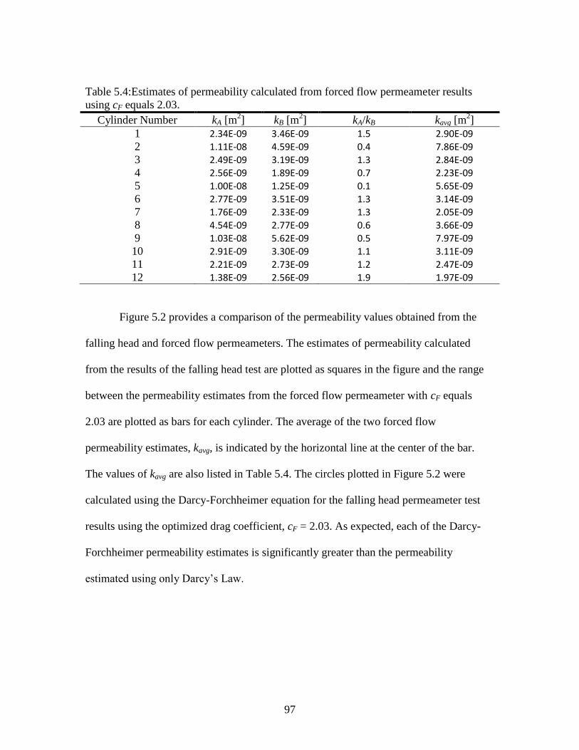
97

Table 5.4:Estimates of permeability calculated from forced flow permeameter results

using cF equals 2.03.

Cylinder Number kA [m2] kB [m

2] kA/kB kavg [m

2]

1 2.34E-09 3.46E-09 1.5 2.90E-09

2 1.11E-08 4.59E-09 0.4 7.86E-09

3 2.49E-09 3.19E-09 1.3 2.84E-09

4 2.56E-09 1.89E-09 0.7 2.23E-09

5 1.00E-08 1.25E-09 0.1 5.65E-09

6 2.77E-09 3.51E-09 1.3 3.14E-09

7 1.76E-09 2.33E-09 1.3 2.05E-09

8 4.54E-09 2.77E-09 0.6 3.66E-09

9 1.03E-08 5.62E-09 0.5 7.97E-09

10 2.91E-09 3.30E-09 1.1 3.11E-09

11 2.21E-09 2.73E-09 1.2 2.47E-09

12 1.38E-09 2.56E-09 1.9 1.97E-09

Figure 5.2 provides a comparison of the permeability values obtained from the

falling head and forced flow permeameters. The estimates of permeability calculated

from the results of the falling head test are plotted as squares in the figure and the range

between the permeability estimates from the forced flow permeameter with cF equals

2.03 are plotted as bars for each cylinder. The average of the two forced flow

permeability estimates, kavg, is indicated by the horizontal line at the center of the bar.

The values of kavg are also listed in Table 5.4. The circles plotted in Figure 5.2 were

calculated using the Darcy-Forchheimer equation for the falling head permeameter test

results using the optimized drag coefficient, cF = 2.03. As expected, each of the Darcy-

Forchheimer permeability estimates is significantly greater than the permeability

estimated using only Darcy’s Law.

98

Figure 5.2: Permeability results for forced flow permeameter (bars) and falling head

permeameter test (squares and circles). Square symbols represent results of Darcy’s Law

and circles represent the solution of the Darcy-Forchheimer equation using the optimized

drag coefficient, cF =2.03.

To investigate whether the coefficient cF is inversely proportional to the porosity

of the pervious concrete cylinders, or related in some other way, it was necessary to

determine individual cF values for each of the pervious concrete cylinders. This was done

by substituting the estimate kB for kA into (5.1.8) for each cylinder.

Table 5.5 lists the resulting drag coefficients for each cylinder.

99

Table 5.5: Individual drag coefficient determined for each cylinder.

Cylinder Number k(B) [m2] cF

1 3.46E-09 2.47

2 4.59E-09 1.30

3 3.19E-09 2.30

4 1.89E-09 1.75

5 1.25E-09 0.72

6 3.51E-09 2.28

7 2.33E-09 2.33

8 2.77E-09 1.59

9 5.62E-09 1.50

10 3.30E-09 2.16

11 2.73E-09 2.26

12 2.56E-09 2.76

The resulting drag coefficients, cF, are plotted in Figure 5.3 along with the

measured porosity for each cylinder respectively. Note the porosity values inside of the

red circles indicate those cylinders with both the highest estimated permeabilities and the

greatest difference between estimates kA and kB. These three cylinders are referred to as

outliers throughout the rest of this section. Of these three cylinders, two of the cylinders

have the highest porosities of the 12 cylinders tested and the other cylinder has the lowest

calculated drag coefficient. Otherwise, there does not appear to be any direct relationship

between the drag coefficient and the porosity for each cylinder.

100

Figure 5.3: Plot of drag constant and porosity for pervious concrete cylinders porosity

values plotted as squares and drag constant values plotted as circles. The red circles

indicate the porosity values for cylinder numbers 2, 5, and 9 which produce extreme

differences in permeability estimates for force flow permeameter experiments as seen in

Figure 5.2.

Figure 5.4 shows the calculated drag coefficient, cF, and the porosity plotted on

the vertical and horizontal axis respectively for each of the twelve cylinders tested.

Likewise, Figure5.5 shows the relationship of the average permeability, kavg, to the

calculated drag coefficient, cF. Again, the outlier values for cylinders 2, 5, and 9 are

circled in red.

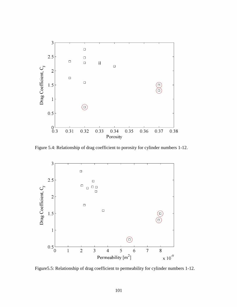
101

Figure 5.4: Relationship of drag coefficient to porosity for cylinder numbers 1-12.

Figure5.5: Relationship of drag coefficient to permeability for cylinder numbers 1-12.

102

Inspection of Figure 5.4 and Figure5.5 suggests that the data, aside from the three

cylinders considered to be outliers, is clustered. There is some indication that the drag

coefficient decreases with increasing porosity; however, many more test would need to

be performed before a relationship between the two properties could be accurately

determined.

The estimates of permeability for cylinders 2, 5, and 9 have been omitted from Figure 5.6

so that the estimates for the other 9 cylinders with similar measures of permeability can

be seen in finer detail. Again, the black bars indicate the minimum, maximum, and

average estimates of permeability obtained from the forced flow permeameter results

using the optimized drag coefficient, cF = 2.03. The squares indicate the estimate of

permeability using Darcy’s Law; the circles indicate the permeability estimate obtained

using the Darcy-Forchheimer equation with cF = 2.03; and the triangles indicate the

permeability estimate found using the Darcy-Forchheimer equation with the calculated cF

values from

Table 5.5. Note that the Darcy and Darcy-Forchheimer approximations are all

calculated using the results of the falling head experiments; however the drag coefficient,

cF, needed to calculate the Darcy-Forchheimer equation was taken from the forced flow

permeameter results. The figure shows that there is wide disagreement in the estimated

values of permeability; however, it does appear that a drag coefficient of 2.03 provides an

estimate of permeability, when using the Darcy-Forchheimer equation with the falling

head test that falls within the range of permeabilities estimated using the forced flow

permeameter method.

103

Figure 5.6: Permeability results for forced flow permeameter (bars) and falling head

permeameter test (squares and circles) with outliers removed. Square symbols represent

results of Darcy’s Law and circles represent the solution of the Darcy-Forchheimer

equation using calculated cF values.

5.3 Conclusions

Three basic conclusions can be made of these preliminary study findings. First, it

appears that the Forchheimer non-linear term is important to the accurate measurement of

permeability. Second, the optimized drag coefficient, cF = 2.03, moves falling head data

into the range measured by forced flow permeameter, or at least much closer to that

range. Third, it is clear that additional research will be required to determine appropriate

values of cF for pervious bicycle lane construction materials.

104

CHAPTER SIX

SUMMARY AND CONCLUSIONS

Bicycles have proven to be an efficient and reliable form of transportation in

urban settings. The addition of bicycle lanes into the transportation network could

significantly impact and improve the sustainability of our urban infrastructure.

Furthermore, incorporating pervious pavements and other low impact development (LID)

strategies into a bicycle lane designs, could both reduce the quantity of stormwater runoff

and improve the quality of stormwater throughout the Waters of the State.

Practicing engineers need both a design aid and research supported methods for

designing these improvements before they can be fully implemented throughout the state

and country. The data and results presented in this thesis have accomplished three main

objectives. 1) The effects of slope on surface infiltration rates of pervious pavements due

to run-on from adjoining impervious traffic lanes was analyzed and a design procedure

for surface infiltration was presented; 2) the characteristics of sub-surface flow for

multiple slope, flow rate, and discharge weir conditions were analyzed and a design

procedure for the bicycle lane subbase was presented; and 3) a preliminary investigation

of an improved test method was completed to determine the permeability of pervious

materials which could be used for bicycle lane construction.

The results of the surface flow experiments, discussed in Chapter 3, provide the

engineer with a method of determining the required hydraulic conductivity and lane

width necessary to infiltrate both the rainfall falling directly on the pervious bicycle lane

surface and the run-on produced by the adjacent impermeable area of the road surface.

105

Figure 3.4 shows a simplified typical cross-section of a pervious bicycle lane located

adjacent to an impervious traffic lane. Given the traffic lane width, wL, the bicycle lane

width, wB, and the rainfall intensity, i, of the design storm event; the required hydraulic

conductivity, Kreq, to prevent ponding of the runoff can be calculated using (3.4.3) when

designing the pervious pavement. Alternatively, the required bicycle lane width, wB,req,

can be calculated using (3.4.4) when the hydraulic conductivity, K, of the pervious

pavement is known.

A method for designing the aggregate subbase layer was provided in Chapter 4,

based on the results of the sub-surface flow experiments. The design method was

discussed for the specific case using a combination of weirs and level bottomed reservoir

areas formed by creating a stair-stepped subbase as seen in Figure 1.1 (d) and also in

Figure 4.9. First, the weir height for each reservoir cell should be set to meet local

drawdown time, Td, requirements using (4.5.1). Next, the length of each cell and thus the

location of each weir should be determined to meet topographical, maximum depth of

cut, costs or other such constraints. Then, the bicycle lane can be routed as a series of

cascading reservoirs, Figure 4.9, with rectangular weir outlets using (4.5.3), (4.5.4), and

(4.5.5). It was determined that the discharge from a rectangular weir with its crest located

within the aggregate sub-base can be approximated using the standard weir discharge

equation (4.1.12) scaled by the aggregate porosity yielding (4.1.14). Finally, the

minimum depth of aggregate base at each weir is obtained by summing the height of the

weir, P, the estimated head above the weir, H, and the allowance of freeboard (4.5.6).

106

Finally, Chapter 5 presented the preliminary findings of a study to improve the

current methods for determining the permeability of the pervious materials used in the

construction of bicycle lanes. Currently, the preferred method for determining the

permeability, via the hydraulic conductivity, of pervious pavements is the falling head

test method ASTM D5856-95 – Test Method B. However; results of the forced flow

permeameter test indicate that the permeability may be 2 to 3 times that obtained using

Darcy’s Law alone. Further research is necessary to determine an expression or

relationship for the drag coefficient, cF, necessary to compute the result of the Darcy-

Forchheimer equation.

Together, these findings show that a conservative hydraulic design for a pervious

pavement bicycle lane is easily accomplished using a few simple formulas and iterative

routines. These methods can be used by practicing engineers to satisfy current regulatory

requirements allowing pervious pavement bicycle lanes to be utilized in place of

traditional drainage systems. While there is still room for improvement, these findings

advance current practice by providing a design method for a simplified case that can be

later modified or expanded as further applications are designed and investigated.

Additionally, these findings may be used for other applications including infiltration

trenches or parking areas where pervious pavements are used on sloped areas.

Future research outcomes could include further study of an improved method to

determine the permeability of pervious pavement construction materials. Also, a better

understanding of the clogging potential of pervious pavements must be investigated

before the use of pervious pavement will be considered for direct runoff capturing

107

applications as described for the bicycle lane. Finally, the interaction between a pervious

bicycle lane system and the adjacent roadway must be addressed, if a pervious bicycle

lane system is to be used directly adjacent to the travel lane, to ensure that the integrity of

the road subbase is not compromised due to the water retained in the subbase layer of the

bicycle lane.

108

REFERENCES

Akan, A. O. (2002). "Sizing stormwater infiltration structures." Journal of Hydraulic

Engineering-Asce, 128(5), 534-537.

Bean, E. Z., Hunt, W. F., and Bidelspach, D. A. (2007a). "Field survey of permeable

pavement surface infiltration rates." Journal of Irrigation and Drainage Engineering-

Asce, 133(3), 249-255.

Bean, E. Z., Hunt, W. F., and Bidelspach, D. A. (2007b). "Evaluation of four permeable

pavement sites in eastern North Carolina for runoff reduction and water quality impacts."

Journal of Irrigation and Drainage Engineering-Asce, 133(6), 583-592.

Chen, L., and Young, M. H. (2007). "Green-Ampt infiltration model for sloping

surfaces." Water Resour.Res., 42(7), W07420.

Coughlin, J. P., Campbell, C. D., and Mays, D. C. (2012). "Infiltration and Clogging by

Sand and Clay in a Pervious Concrete Pavement System." J.Hydrol.Eng., 17(1), 68-73.

Deo, O., Sumanasooriya, M., and Neithalath, N. (2010). "Permeability Reduction in

Pervious Concretes due to Clogging: Experiments and Modeling." J.Mater.Civ.Eng.,

22(7), 741-751.

Dietz, M. E. (2007). "Low impact development practices: A review of current research

and recommendations for future directions." Water Air and Soil Pollution, 186(1-4), 351-

363.

Dreelin, E., Fowler, L., and Carroll, C. (2006). "A test of porous pavement effectiveness

on clay soils during natural storm events." Water Res., 40(4), 799-805.

Eisenberg, B. (2010). Low Impact Development 2010: Redefining Water in the City.

Emerson, C. H., and Traver, R. G. (2008). "Multiyear and seasonal variation of

infiltration from storm-water best management practices." Journal of Irrigation and

Drainage Engineering-Asce, 134(5), 598-605.

Essig, E. T., Corradini, C., Morbidelli, R., and Govindaraju, R. S. (2009). "Infiltration

and deep flow over sloping surfaces: Comparison of numerical and experimental results."

Journal of Hydrology, 374(1-2), 30-42.

Federal Highway Administration. (2009). "Urban Drainage Design Manual. Hydraulic

Engineering Circular No. 22, Third Edition. (HEC-22." FHWA-NH1-10-009.

109

Ferguson, B. K. (1994). Stormwater Infiltration. Lewis Publishers, Boca Raton, Florida.

Gupta, R. S. (2008). "Hydraulic Principles of Structures." Hydrology and Hydraulic

Systems, Third Edition, Waveland Press, Inc., Long Grove, Illinois, 533.

Haselbach, L. M. (2010). "Potential for Clay Clogging of Pervious Concrete under

Extreme Conditions." J.Hydrol.Eng., 15(1), 67-69.

Hayes, J., Godbold, E., and Barfield, B. (2001). "Turbidity Based on Sediment

Characteristics for Southeaster U.S. Soils." Soil Erosion Research for the 21st Century,

International Symposium, Honolulu, Hawaii, 408--411.

Horst, M. (2011). "Multiyear Performance of a Pervious Concrete Infiltration Basin

BMP." J.Irrig.Drain.Eng., 137(6), 352-358.

Kwiatkowski, M., Welker, A. L., Traver, R. G., Vanacore, M., and Ladd, T. (2007).

"Evaluation of an infiltration best management practice utilizing pervious concrete."

J.Am.Water Resour.Assoc., 43(5), 1208-1222.

Luck, J. D., Workman, S. R., Higgins, S. F., and Coyne, M. S. (2006). "Hydrologic

properties of pervious concrete." Transactions of the Asabe, 49(6), 1807-1813.

Matel, L. (2010). Low Impact Development 2010: Redefining Water in the City.

Nield, D. A., and Bejan, A. (2006). Convection in Porous Media, Springer Science and

Business Media, Inc., New York, 1-14.

Paige, G. (2002). "A strip model approach to parameterize a coupled green-ampt

kinematic wave model." J.Am.Water Resour.Assoc., 38(5), 1363-1377.

Pitt, R., Chen, S., Clark, S. E., Swenson, J., and Ong, C. K. (2008). "Compaction's

impacts on urban storm-water infiltration." Journal of Irrigation and Drainage

Engineering-Asce, 134(5), 652-658.

Pitt, R., and Clark, S. E. (2008). "Integrated storm-water management for watershed

sustainability." Journal of Irrigation and Drainage Engineering-Asce, 134(5), 548-555.

Sansalone, J., Kuang, X., and Ranieri, V. (2008). "Permeable pavement as a hydraulic

and filtration interface for urban drainage." Journal of Irrigation and Drainage

Engineering-Asce, 134(5), 666-674.

Schwartz, S. S. (2010). "Effective Curve Number and Hydrologic Design of Pervious

Concrete Storm-Water Systems." J.Hydrol.Eng., 15(6), 465-474.

110

Siriwardene, N. R., Deletic, A., and Fletcher, T. D. (2007). "Clogging of stormwater

gravel infiltration systems and filters: Insights from a laboratory study." Water Res.,

41(7), 1433-1440.

Stone, J. J. (1992). "Infiltration and runoff simulation on a plane." Trans.ASAE, 35(1),

161-170.

Tosomeen, C. (2008). "Pervious Concrete Bicycle Lanes — Roadway Stormwater

Mitigation within the Right-of-Way." Low Impact Development for Urban Ecosystem

and Habitat Protection, 23-23.

Vulcan Materials. (2013). "Construction Materials." http://www.vulcanmaterials.com/

(March 8, 2013).