Template

A Methodology for Delineating Planning-Level Channel Migration Zones

July 2014 Publication no. 14-06-025

Publication and Contact Information

This report is available on the Department of Ecology’s website at https://fortress.wa.gov/ecy/publications/SummaryPages/1406025.html For more information contact: Shorelands and Environmental Assistance P.O. Box 47600 Olympia, WA 98504-7600

Phone: (360) 407-6966

Washington State Department of Ecology - www.ecy.wa.gov

o Headquarters, Olympia 360-407-6000

o Northwest Regional Office, Bellevue 425-649-7000

o Southwest Regional Office, Olympia 360-407-6300

o Central Regional Office, Yakima 509-575-2490

o Eastern Regional Office, Spokane 509-329-3400 Cover photo: Lower Elwha River I f you need this document in a format for the visually impaired, call the Shorelands and Environmental Assistance at (360) 407-6966. Persons with hearing loss can call 711 for Washington Relay Service. Persons with a speech disability can call 877-833-6341.

A Methodology for Delineating Planning-Level Channel Migration Zones

by;

Patricia L. Olson & Nicholas T. Legg Washington Department of Ecology

Tim B. Abbe & Mary Ann Reinhart

Natural Systems Design

Judith K. Radloff Geoengineers, Inc.

Shorelands and Environmental Assistance Program Washington State Department of Ecology

Olympia, Washington

i

Table of Contents Page

Table of Contents ................................................................................................................. i

List of Figures and Tables................................................................................................... ii Figures........................................................................................................................... ii Tables ............................................................................................................................ ii

List of Acronyms ............................................................................................................... iii

Acknowledgements ............................................................................................................ iv

Abstract ................................................................................................................................v

Summary ............................................................................................................................ vi

Introduction ..........................................................................................................................1 CMZ mapping ................................................................................................................1 Channel migration processes .........................................................................................3 Regulatory context .........................................................................................................6

Shoreline Management Act ...................................................................................7 Other Washington regulations ...............................................................................8 NWF v. FEMA Federal legal decision ..................................................................8

Planning-level methodology background ......................................................................8 Planning-level CMZ methodology development ...........................................................9

Planning-Level CMZ Delineation Methodology ...............................................................10 General principles and approach ..................................................................................11 The analyst ...................................................................................................................12 Local knowledge ..........................................................................................................12 Planning-level CMZ map unit definitions ...................................................................12 GIS data sources and processing ..................................................................................13

Topography ..........................................................................................................13 Aerial imagery .....................................................................................................14 Other geospatial data ...........................................................................................15

Mapping the pCMZ ......................................................................................................17 Reach delineation (Data Sheet Section 1, Appendix A) ......................................17 Modern Valley Bottom mapping (Data Sheet Section 2, Appendix A) ..............19 Avulsion Hazard Area mapping (Data Sheet Section 3, Appendix A) ...............23 Erosion Hazard Area mapping (Data Sheet Section 3, Appendix A) ..................25 Disconnected Migration Area mapping (Data Sheet Section 4, Appendix A) ....30 Mapping of other units (Data Sheet Section 4, Appendix A) ..............................31 Planning-Level CMZ mapping in unconfined valleys with minimal migration .32

Recommended QA/QC review ....................................................................................33 Method limitations .......................................................................................................33

References Cited ................................................................................................................35

ii

Appendices .........................................................................................................................40 Appendix A. Reach Datasheet .....................................................................................41 Appendix B. Example Planning-Level CMZ Delineations .........................................42 Appendix C. Comparison of planning to detailed CMZ delineations .........................48 Appendix D. Relevant Washington State Regulations ................................................52 Appendix E. Methods for Generating Relative Elevation Models ..............................56

List of Figures and Tables Page

Figures Figure 1. Example of channel migration on the Lower Elwah River (WA) ........................4 Figure 2. Illustration of channel avulsion classification ......................................................5 Figure 3. Example of channel widening ..............................................................................6 Figure 4. Visualizing floodplain landforms using different remotely-sensed data ............15 Figure 5. Schematic diagram of a pCMZ ...........................................................................18 Figure 6. Conceptual diagram on determining EHA-width ...............................................27 Figure 7. Cross-sectional illustration of geotechnical hazards and pCMZ map units .......30 Figure 8. CMZs versus FEMA floodplains .......................................................................32

Tables Table 1. Required map units of the pCMZ. .......................................................................12 Table 2. Sub-map units and flags likely used in the pCMZ method. .................................13 Table 3. Other units mapped. .............................................................................................13 Table 4. Information on geospatial data used in the pCMZ method. ................................16

iii

List of Acronyms CMZ Channel Migration Zone DEM Digital Elevation Model DMA Disconnected Management Area DNR Washington State Department of Natural Resources DOQQ Digital Orthophotos by Quarter Quadrangle DRG Digital Raster Graphics Ecology Washington Department of Ecology EHA Erosion Hazard Area (pCMZ) EPA Environmental Protection Agency (US) FEMA Federal Emergency Management Agency GIS Geographical Information Systems LiDAR Light Detection and Ranging MVB Modern Valley Bottom (pCMZ) NAIP National Aerial Imagery Program NED National Elevation Dataset NMFS National Marine Fisheries Service NOAA National Oceanic and Atmospheric Administration (US) pCMZ Planning-Level Channel Migration Zone QAQC Quality Assurance/Quality Control Qal Quaternary Alluvium deposits (unit on geologic map approximating MVB) Qls Quaternary Landslide deposits REM Relative Elevation Model SMA Washington State Shoreline Management Act SMP Washington State Shoreline Management Plan USGS United States Geological Survey UW University of Washington WAC Washington Administrative Code

iv

Acknowledgements The authors of this report would like to thank the United States Environmental Protection Agency, Region 10 for their support. The authors also would like to thank the following people for their thoughtful reviews of earlier drafts of this report:

• Janine Castro, National Oceanic and Atmospheric Administration - National Marine Fisheries Service, Portland, Oregon

• Chuck Dalby, Montana Department of Natural Resources and Conservation

• Thomas Dunne, University of California, Santa Barbara

• Christopher Konrad, U.S. Geological Survey, Tacoma, Washington

• Jim O’Connor, U.S. Geological Survey, Portland, Oregon

• Paul Pittman, Element Solutions, Bellingham, Washington

• Betty Renkor, Washington Department of Ecology

This project has been funded wholly or in part by the United States Environmental Protection Agency under assistance agreement PC-00J281-02 to Department of Ecology. The contents of this document do not necessarily reflect the views and policies of the Environmental Protection Agency, nor does mention of trade names or commercial products constitute endorsement or recommendation for use.

v

Abstract The Washington State administrative codes that implement the Shoreline Management Act (SMA) require communities to identify the general location of channel migration zones (CMZs), and regulate development within these areas on shoreline streams. Shoreline streams are defined as those with a mean annual flow equal to or greater than 20 cfs. While many channel migration studies and CMZ delineations have been done in Washington State, nearly all have been detailed assessments. These CMZ delineations are more rigorous then required by the state SMA administrative codes, which emphasize planning-level assessments. The rigorous studies are cost-prohibitive to implement for all regulated shoreline streams in the state. The SMA and its administrative codes provide no guidance on planning-level CMZ delineation methods. The Washington Department of Ecology (Ecology) developed a planning-level CMZ delineation (pCMZ) method to support local communities’ updates and implementation of the SMA requirements. Ecology developed the pCMZ method through a process of: (1) initial pCMZ method development; (2) application and refinement of the method over 900 stream miles near the Puget Sound; and, (3) further refinement through comparison of CMZs mapped using the planning-level approach to CMZs mapped using detailed CMZ methods. The pCMZ method uses the nature and extent of valley bottom features to assess past and potential future channel migration, and then define CMZ boundaries. This document describes the pCMZ approach in context of Washington State regulations.

vi

Summary Dynamic physical processes in streams can cause channels to move laterally or "migrate" over time (Figure 1). The area that a stream channel has historically occupied and is reasonably likely to move over some time (defined by the user) is referred to as the channel migration zone (CMZ). CMZs delineate areas with hazards from migrating stream channels, and therefore serve as a template for mitigating risk. They also allow for protection and restoration of the productive floodplain habitat that channel migration creates (Ward and Stanford, 1995a; Abbe and Montgomery, 1996; Beechie and Bolton, 1999; Collins et al., 2012). This document outlines a relatively low-cost method to CMZ mapping that accounts for variation in fluvial processes and channel migration along streams. The method uses landforms and characteristics of the valley bottom to evaluate past channel migration activity and define a CMZ. The emphasis on landforms and valley characteristics accounts for local variations on channel migration potential while avoiding detailed quantitative analyses. Because the method is best applied over relatively large areas for planning purposes, it is termed the planning-level CMZ (pCMZ) delineation methodology. While less-detailed than some other CMZ methods, the pCMZ approach identifies the general location of the CMZ as required under Washington State Administrative Codes (notably WAC 173-26-201) implementing the Shoreline Management Act (SMA). The associated administrative codes require that communities updating their Shoreline Master Programs (SMPs) map CMZs for all streams equal to or exceeding 20 cubic feet per second mean annual flow. The low-cost approach outlined here facilitates CMZ mapping of the many thousands of stream miles within SMA jurisdiction currently unmapped. The analyst mapping the pCMZ should particularly have experience with interpreting landforms with aerial imagery and other remotely sensed data. Due to the dependence on the landform interpretation, the analyst’s past experience in fluvial geomorphology is as critical for the pCMZ methods as for detailed CMZ methods that utilize channel migration rate measurements Professional Geologist and Engineer licenses alone do not necessarily indicate the requisite experience for pCMZ mapping. In addition to a professional license, the analyst should have at least five years experience in applied fluvial geomorphology. In cases where geotechnical questions are encountered during pCMZ delineation, fluvial geomorphologists should consult with licensed geologists and engineers with expertise in slope stability and geotechnical properties of earth materials. The pCMZ method is based on the simple premise that the channel, floodplain, and valley bottom reflect the activity and spatial influence of channel migration. The channel, floodplain, and valley bottom provide a record of past channel migration, and a baseline for evaluating future channel migration. The method uses readily available remotely sensed topography and aerial imagery, as well as publically available geospatial data such as soils and geologic maps to identify portions of the valley in the pCMZ. Channel migration records preserved in landforms, soils, and geology are the basis for the pCMZ delineation. The pCMZ delineation approach consists of two core steps:

vii

• Identify the Modern Valley Bottom where channel migration has occurred and is likely to occur.

• Assess the potential influence of channel migration on the areas adjacent to the modern valley bottom, and delineate Erosion Hazard Areas accordingly.

The fundamental component of the pCMZ is the Modern Valley Bottom (MVB), which encompasses the area where channel migration has occurred in the past few thousand years. Because channels often migrate into areas they have previously occupied, the MVB will account for much of the pCMZ width needed for future migration (O’Connor et al., 2003; Konrad, 2012). For areas where there is potential for widening of the MVB from lateral erosion, Erosion Hazard Areas are mapped along the outer limit of the MVB. Therefore, the Modern Valley Bottom plus the Erosion Hazard Area defines the pCMZ, the area where channel migration is reasonably likely to occur in the current climatic and hydrologic regime. Because the pCMZ method does not use channel migration rate measurements, the pCMZ delineation cannot be assigned a numerical design life. For this reason, the qualitative design life of the pCMZ definition is the “current climatic and hydrologic regime,” which is considered to be greater and more conservative than the 100- or 500-year design periods typical for detailed CMZ assessments. Additional, but not always present, map units include the Avulsion Hazard Area, a unit within the MVB, and the Geotechnical Flag, which indicates slope stability hazards resulting from lateral channel erosion. In addition, areas disconnected by man-made erosion barriers such as levees are mapped outside of the CMZ as Disconnected Migration Areas. While outside of the pCMZ, Disconnected Migration Areas provide an inventory of potential floodplain restoration opportunities. Other units mapped outside the pCMZ are Potential Inundation Zones and alluvial fans. Appendixes contain supporting information, tools, and methods. • Appendix A contains a Data Sheet for recording information during the pCMZ delineation. • Appendix B provides example pCMZ delineations. • Appendix C outlines an evaluation of the pCMZ method relative to more detailed CMZ

methods. • Appendix D outlines the Washington State regulations relating to channel migration. • Appendix E outlines methods for creation of Relative Elevation Models, a landform

visualization technique essential to the pCMZ method.

1

Introduction Dynamic physical processes in streams can cause channels to move laterally or migrate over time (Figure 1). The area within which a stream1 channel has historically occupied and is reasonably likely to move over some time (defined by the user) is referred to as the channel migration zone (CMZ). The width of a CMZ may sometimes only be slightly larger than a channel width, but for many alluvial channels with their bed composed of sediment, the CMZ’s width is often many times that of the stream. The CMZ may include the entire valley bottom and even extend into adjacent hillslopes for some streams. Channel migration poses a hazard to infrastructure and communities, yet generates topographic and biologic complexity in floodplains that provides habitat for fish and fauna (Ward and Stanford, 1995a; Abbe and Montgomery, 1996; Beechie and Bolton, 1999; Collins et al., 2012). Defining CMZs and regulating development within their boundaries, therefore, can help to minimize risk and maintain biologically productive floodplains. Channel migration provides critical habitat and benefits to riparian areas (Ward and Stanford, 1995b; Florsheim et al., 2008). Channel migration is an important geomorphic process that creates a shifting mosaic of habitat patches of different ages within the river corridor (Fetherston et al., 1995). This mosaic provides highly productive ecological areas for aquatic organisms as well as terrestrial species. Channel migration processes occur on a variety of spatial and temporal scales from local bank erosion to avulsions that create many kilometers of new channel to entire reworking of floodplains. Streams erode some patches each year while other patches accrete sediment and gradually rise in elevation above the river bed (Nanson and Beach, 1977; Abbe and Montgomery, 1996; Brummer et al., 2006; Collins et al., 2012). The high density of complex boundaries between ecotones creates more environmental complexity, maintained by interactions between river channels and floodplain forests (Ward et al., 1999).

CMZ mapping While a number of CMZ definitions and delineation methods exist, a method established by Rapp and Abbe (2003) (https://fortress.wa.gov/ecy/publications/summarypages/0306027.html) is the most often used in Washington State. The method developed by Rapp and Abbe defines a CMZ as a composition of zones; the Historical Migration Zone, Avulsion Hazard Zone, Erosion Hazard Zone, and the Disconnected Migration Area. • The Historical Migration Zone is the area the stream channel has occupied over the time

period spanning the historical record. Historical maps and aerials serve as the record of previous stream channel locations.

• The Avulsion Hazard Zone is an area deemed susceptible to avulsion of the main stem channel. Avulsions are abrupt switches in channel course that can have catastrophic consequences for existing floodplain development. Avulsion Hazard Zones may include low-

1 In this document the term stream is used for all flowing water within a naturally created channel. For example brooks, creeks, spring brooks, and rivers are all considered streams.

2

lying floodplain areas capable of capturing main stem flows, and areas between channel bends prone to avulsions that cutoff meander bends.

• The Erosion Hazard Zone is an area outside the Historical Migration Zone that has a reasonable likelihood to be influenced by channel migration over the design life of the CMZ. A CMZ‘s Erosion Hazard Zone often extends outside and above the Federal Emergency Management Agency’s (FEMA’s) flood zones along actively migrating streams. The Erosion Hazard Zone includes up to two components: an Erosion Setback, and a Geotechnical Setback.

o The Erosion Setback is the projection of channel migration rates into the future, based on the average rate of migration documented from dated time series of aerial photographs and surveyed maps. Where the Erosion Setback overlaps hillslopes or landforms prone to slope failure, a Geotechnical Setback is mapped.

o A Geotechnical Setback identifies the likely area that would be impacted by potential slope failure. Geotechnical Setbacks are delineated where the channel is migrating or could migrate into the valley wall or elevated landforms such as stream terraces. The high terrace actively being eroded by the channel shown in Figure 1 is an example where geotechnical setbacks would be required.

• Disconnected Migration Areas are mapped in certain scenarios where levees or other infrastructure disconnect an area of the CMZ from its natural extent.

Existing CMZ delineation techniques like the methods of Rapp and Abbe (2003) involve detailed analysis of historical channel migration, and therefore are often best-suited for site- and reach-specific projects. Despite the long-term benefits that these detailed CMZ maps can provide, mapping is often too expensive to apply over many miles of channel. Therefore, a lower-cost alternative that provides a conservative estimate of a CMZ is needed. A conservative CMZ, by definition, could provide greater protection and reduction in damages from migrating channels at a lower cost than more robust analyses. Previous efforts to develop low-cost CMZ delineation methods have often involved empirical relationships or corridor definitions that do not account for varying fluvial processes along streams. Locally in the Puget Sound Region, Skidmore et al. (1999) proposed integrating the limits of historical channels, geologic controls, and the 100-year floodplain. While this method likely provides a conservative estimate of CMZ, it also requires the process of mapping historical channels. Other delineation methods have involved empirical relationships between channel size and meander amplitude (Piégay et al., 2005). Despite minimal costs, simple empirical relationships cannot account for local variations in channel pattern, valley type, and migration activity. This document outlines a relatively low-cost method to CMZ mapping that accounts for variation in fluvial processes and channel migration along streams. The method uses landforms and characteristics of the valley bottom to evaluate past channel migration activity and define a CMZ. The emphasis on landforms and valley characteristics accounts for local variations in channel migration potential. Because the method is best applied over relatively large areas for planning purposes, it is termed the planning-level CMZ (pCMZ) delineation methodology.

3

Channel migration processes Channel migration occurs through processes of channel expansion, gradual bend migration, and abrupt channel switching termed avulsions (Knighton, 1998). While the physical mechanisms of each migration process are different, the processes are often intertwined. For instance, avulsions occurring across meander bends (termed meander bend cutoffs) are a direct result of gradual bend migration. Gradual channel migration and abrupt avulsions should therefore be considered together under the overall process of channel migration. Channel widening is a process that can occur naturally, as well as because of clearing of riparian vegetation (e.g. Brooks and Brierley, 2002; Brooks et al., 2003; Eaton, 2006). It can occur episodically in response to floods (Konrad, 2012), or as a long-term change due to increases in surface water runoff resulting from upland development or climate change. Channel migration occurs in three dimensions through time. Channels not only move laterally, but also vertically. Vertical changes directly affect lateral changes. For example, when a channel cuts downward (incises) such as occurs in response to increases in peak flows or channel straightening, it can slow lateral migration temporarily but may ultimately lead to more severe bank erosion and destabilization of adjacent hillslopes (Simon, 1989; Booth et al., 2004). When a channel bed rises, or aggrades, from sediment deposition, channel migration is generally more likely (Dunne et al., 2010). Channel aggradation can also cause rapid migration when the rate of sediment deposition is high, as in the case of deposition resulting from large debris flows and landslides. Gradual migration of meander bends occurs when flow within a stream has sufficient energy to erode banks on the outside of meander bends. Lateral accretion (deposition) of sediment occurs simultaneously on the inside of channel bends (Figure 1.1). Lateral channel migration is dependent on the ability of bank soils to resist erosion by stream flow (Nanson and Croke, 1992). The rate of bend migration generally increases with discharge, velocity and duration of stream flows exceeding a threshold condition; for example, migration rates are generally greatest during floods (Konrad, 2012). Channel migration also can occur as the channel abruptly switches its course, referred to as channel avulsion. Avulsions differ in their frequency and size, and thus have varying levels of hazard (Figure 2). Meander cutoff avulsions create new channels between adjacent bends, and therefore impact a relatively small area of the floodplain (Slingerland and Smith, 2004). However, because channel bends scale with the size of a stream (Leopold and Wolman, 1960), the impact of a single meander bend cutoff can be significant in large streams. Valley-scale avulsions form new channels that can extend long distances downstream. Avulsions vary in their frequency, as well. Meander cutoffs typically occur on yearly to decadal timescales in migrating channels and are a natural and regular response to channel lengthening resulting from gradual bend migration (Constantine and Dunne, 2008). Valley-scale avulsions have recurrence intervals on the order of hundreds to thousands of years (Makaske et al., 2002; Slingerland and Smith, 2004; Tooth et al., 2007). Valley-scale avulsions have not been recorded historically in the Puget Sound, but geological records reveal valley -scale avulsions within the

4

last few thousand years (Pittman and Maudlin, 2003). Depending on a valley’s morphology and geologic history, valley-scale avulsions may be possible (Collins and Montgomery, 2011). Avulsions are also common on particular landforms and in channels with particular patterns. Deltas and alluvial fans form as a result of many avulsions through time. Another avulsion common to anabranching streams occurs when streams switch back and forth between channels or into floodplain sloughs (relict channels) and reconnect with the main channel farther downstream (Collins et al 2003, Collins et al 2012). Often this avulsion process creates forested islands between channels. These two kinds of avulsions tend to be more local and can occur regularly during floods.

Figure 1. Example of channel migration on the Lower Elwah River (WA). A series of aerial photographs of the Lower Elwha River (WA) demonstrates migration from lateral accretion on inside bend and bank erosion on the outside bend. These aerial photographs also illustrate hazardous and beneficial consequences of channel migration. The photographs show habitat creation (side channel) by migration processes and document a property and the encroachment of the channel through time (home in yellow for reference). Despite being located on a Quaternary glacial terrace over 120 ft (40 m) above the river, the eroding embankment has advanced dangerously close to the house. Between 1990 and 2013 the river migrated 145 ft (44 m) to the west and within 55 ft (17 m) of the home. Even if channel migration were to stop now, natural adjustment of the unstable embankment (mass wasting) would continue to place the house at very high risk.

5

Figure 2. Illustration of channel avulsion classification.A hierarchical classification of channel avulsions plotted by length-scale, where length is measured as the length of channel formed by an avulsion (shaded grey). Active, post-avulsion channels (black) and inactive channels abandoned at the time of avulsion (grey outlines) illustrate the style and length-scale of each avulsion type. Local and valley-scale avulsions define the most basic division. Valley-scale avulsions are similar to ‘regional’ avulsions discussed by Slingerland and Smith (2004).. Meander cutoffs, a form of local avulsions, are relatively regular occurrences in actively migrating streams, and are classified as neck and chute cutoffs. Island-forming avulsions are defined here as avulsions that form forested islands in floodplains, and are common in watersheds and floodplains dominated by old-growth forests that generate large log jams that induce avulsions (Abbe and Montgomery, 1996; Collins et al., 2012). Valley-scale avulsions tend to occur when streams deposit material over geologic timescales and form alluvial ridges that create steep gradients away from the channel (Slingerland and Smith, 2004). Channel widening can also occur and is often associated with major flood events or increases in discharge resulting from urbanization common throughout Western Washington (Konrad and Booth, 2002; Konrad et al., 2011). Figure 3 shows a residential development with homes built next to a stream that has widened considerably between 1990 and 2009. The 2009 image shows that the stream in this residential development moved, eroded banks, deposited sediment, and

6

removed trees and vegetation along the banks. The loss of vegetation along the stream banks may further increase the likelihood that the channel will widen and migrate further. The extent of areas historically occupied by channels does not necessarily predict where channels will migrate in the future. For example, the O’Connor et al. (2003) channel migration analysis on the Quinault and Queets Rivers in the Olympic Mountains found that 40% to 50% of the channel migration occurred in areas on the floodplain that the channel had not occupied historically. Channels can also migrate outside of historical migration zones in response to upstream changes such as land development or forest management, which may alter the routing of sediment and wood and change flow regimes (Jones and Grant, 1996; Konrad and Booth, 2002; Booth et al., 2004). For greater detail on channel migration processes and patterns in Western Washington, refer to a Washington Department of Ecology publication (no. 14-06-028) found at the Ecology publications webpage https://fortress.wa.gov/ecy/publications/SummaryPages/1406028.html.

Figure 3. Example of channel widening. Mission Creek near Belfair, WA illustrates channel widening between 1990 and 2009, and its encroachment on the adjacent community.

Regulatory context CMZ mapping in Washington is driven by State shoreline and floodplain management regulations as well as a Federal legal decision.

Mission Creek

7

Shoreline Management Act The Washington State Department of Ecology (Ecology) is the state agency responsible for regulating shoreline and floodplain development through its Shoreline Management Act (SMA) of 1971 (Chapter 90.58 RCW) and implementing rules. The SMA’s policies include both protecting shoreline resources of the state while allowing appropriate and reasonable land use of shorelines. The SMA directs Ecology to develop appropriate administrative codes and to provide assistance to local communities for updating Shoreline Master Programs and ordinances for both freshwater and coastal areas. The Washington Administrative Code (WAC) rules for master program development and updates include the SMP Guidelines (Chapter 173-26 WAC Part III adopted in 2003, amended 2011). The SMPs carry out the policies of the Shoreline Management Act at the local level, regulating use and development of shorelines. Local shoreline programs include policies and regulations based on state laws and rules but tailored to the unique geographic, economic, and environmental needs of each community. The State of Washington recognizes that development in CMZs puts people and investments in harm’s way, requires expensive protection measures, and negatively impacts important habitat for endangered salmon and other species. The State incorporates identifying and regulating CMZs through the SMP Guidelines. The SMP Guidelines address channel migration along shoreline streams (all streams with at least 20 cfs mean annual flow). The Guidelines (WAC 173-26-201(3)(c)(vii)) require a community to identify the “general location of channel migration zones” during the shoreline inventory and characterization phase of the SMP update. The SMP Guidelines provide more detailed information on policies and regulations for CMZs in sections on critical area requirements (WAC 173-26-221(2)(c)(iv)); flood hazard reduction (WAC 173-26-221(3)); modifications WAC 173-26-231(3):, shoreline stabilization (WAC 173-26-231(3), and conditional use for dredge material disposal (WAC 173-26-231(3)(f) and for mining WAC 173-26-241(3)(ii)(E). Appendix C provides Guidelines language and hyperlinks to the WAC sections addressing channel migration.

The flood hazard reduction portion of the SMP Guidelines emphasizes the public safety element (WAC 173-26-221(3)). The Guidelines recognize that channel migration can pose a much greater hazard than flooding alone. Development and shoreline modifications should be limited where they interfere with the channel migration processes and where channel migration could cause significant adverse impact to property, public improvements or people (WAC 173-26-221(3)(b-c)). The SMP Guidelines address management of critical areas designated under the Growth Management Act (GMA) and within shoreline management jurisdiction area. Two provisions of the GMA critical areas regulations include channel migration zones. CMZs are included as erosion hazard areas (WAC 365-190-030(5)) and geologically hazardous areas (WAC 365-190-120(6)(f)).

8

Other Washington regulations The Washington Floodplain Management Program addresses channel migration through Comprehensive Flood Hazard Management Plans developed by local communities. Identification of channel migration zones under SMP criteria may also support community efforts at complying with new FEMA regulations related to endangered species. The FEMA Risk Map program implemented through the Floodplain Management Program incorporates channel migration to align CMZ mapping with the NOAA-FEMA Biological Opinion. Channel migration is also included in state forest practices manual administered by the Washington State Department of Natural Resources. The forest practices manual limits harvest and road building in channel migration areas.

NWF v. FEMA Federal legal decision A Federal legal decision recognizes the importance of channel migration processes in creating critical habitat in the Puget Sound. In accordance with the judicial order in NWF v. FEMA, 345 F. Supp. 2d 1151, the National Marine Fisheries Service (NMFS) Biological Opinion declared that the Federal Emergency Management Agency (FEMA) floodplain management program results in a “take” of Puget Sound Chinook salmon, steelhead and Orca whales (NMFS, 2008). The NMFS opinion allows for reasonable and prudent alternatives to be implemented that would reduce the likelihood of jeopardizing the continued existence of listed species or result in destruction or adverse modification of critical habitat. The NMFS discussed with the FEMA the availability of a reasonable and prudent alternative that the FEMA can take to avoid violation of the Endangered Species Act section 7(a)(2) responsibilities (50 CFR 402.14(g)(5)). Puget Sound communities can demonstrate through a FEMA approved checklist that current community development and land-use requirements such as Shoreline Master Program and other state and local regulatory programs already meet the requirements of National Marine Fisheries Service (NMFS) Biological Opinion reasonable and prudent element 3 and Appendix 4 (FEMA 2010).

Planning-level methodology background The SMP Guidelines require only planning level assessments and delineations of channel migration. Most completed CMZ assessments and delineations in Washington used techniques involving detailed analysis of historical and current conditions to document migration processes, rates and trends of past and present stream movement. Some also included geologic erosion hazards, past channel response prior to development, and estimates of how channel will behave into the future. Detailed channel migration assessment and mapping methods are described in the scientific and grey literature and in Ecology publications (Rapp and Abbe, 2003). A draft Ecology publication includes links to detailed channel migration assessments and CMZ maps (Olson, 2008). The relatively high-cost per stream mile of mapping detailed-level CMZs has caused a large proportion of the stream miles in Washington to be left unmapped. Despite the long-term cost avoidance that CMZs can provide, detailed-assessments are costly and require more information

9

than required by the Shoreline Master Program Guidelines. Thus, the SMP Guidelines only require the identification of the general location of the CMZ. However, the Guidelines provide little technical guidance on how to identify the general location of the CMZ. The SMP Guidelines require communities to only use existing information and data in the watershed characterization and inventory phase of the Shoreline Master Program updates. Consistent with this, the planning level Channel Migration Zone (pCMZ) methodology uses only existing GIS data and does not require field observations or new data. Because the pCMZ is a planning level methodology, the CMZ boundaries will be conservative. Planning level CMZ assessments do not replace detailed-level CMZs. The Shoreline Management Act directs Ecology to provide the scientific basis and technical assistance on delineating regulatory CMZs for the Shorelines Master Program. The planning-level method outlined in this document fulfills those obligations.

Planning-level CMZ methodology development In 2010, the Region 10 USEPA, through the Puget Sound Scientific Studies and Technical Investigations Assistance Program in Support of Implementing the Puget Sound Action Agenda, funded Ecology’s proposal entitled, Channel Migration Assessments: Providing Puget Sound Communities with Information and Technical Assistance for Shoreline Master Programs and Floodplain Management. Development of a planning-level CMZ delineation methodology is an important objective of the project. A two-phase project was initiated to develop and evaluate a CMZ delineation method appropriate for use by SMP communities and others. Phase I included development of the planning-level CMZ delineation methodology (pCMZ) that would meet SMP requirements and be less expensive than available detailed and robust methods. The resulting planning-level CMZ method was applied to approximately 520 stream miles in Clallam, Mason, Kitsap, and Skagit Counties and some small municipalities in other counties in the Puget Sound region of Washington. These are only a subset of all migrating streams in this region. They were chosen based on the local communities’ SMP update schedules. The Quality Assurance Project Plan for the Channel Migration Assessment project required all CMZ maps produced using the pCMZ methodology to be reviewed (Olson and Franklin 2012). Planning-level delineations were supervised and reviewed by senior-level geomorphologists from the consulting team and the Department of Ecology prior to finalization of the maps Although the method was originally developed for use on SMP streams in Puget Sound, the methodology has been applied to streams in non-Puget Sound regions of Washington State. These include approximately 450 stream miles in non-Puget Sound portions of the Olympic Peninsula and central and eastern Washington2.

2 CMZ delineations on these streams were not supported by the USEPA grant for Puget Sound streams but provided additional cases and information to revise the Planning Level CMZ delineation methodology developed under the USEPA grant for Puget Sound streams.

10

The second phase of the project focused on evaluating the results of the pCMZ with respect to CMZs delineated using more robust analyses and more abundant historical data (detailed-CMZs or dCMZ). Objectives of the Phase 2 effort included the following: • Apply the SMP planning level CMZ delineation methodology to a subset of streams with

existing detailed studies. • Evaluate the credibility and usefulness of the planning level CMZ method as compared to

dCMZ maps delineated for a variety of stream types and compare and evaluate differences between the planning level CMZ and dCMZ maps.

• Modify the SMP planning level CMZ assessment based on findings from the comparisons and review by senior-level geomorphologists with extensive experience interpreting fluvial landforms and mapping CMZs.

The original planning-level CMZ delineation methodology (pCMZ) was revised to be more efficient and applicable in other settings. Chapter 2 of this document describes only the modified planning level CMZ approach. Appendix C contains more discussion on a comparison of pCMZ and dCMZs for a subset of Puget Sound streams. The pCMZ is also intended to be used as a floodplain management tool and to identify channel reaches where detailed-CMZ delineations are needed. Other applications for the methodology include the FEMA/state Risk Map program and other hazard assessments, restoration planning, and identification of areas suitable for development or protection. While developed in Washington State, the pCMZ method can be adapted to and applied in other regions.

Planning-Level CMZ Delineation Methodology The planning level CMZ delineation approach (pCMZ ) uses readily available geospatial data to evaluate landforms, stream patterns, and valley bottom characteristics that indicate the level and influence of channel migration activity. The methodology involves only limited analysis of historical channel migration behavior, and is therefore not a substitute for a detailed CMZ assessment. Detailed CMZ assessments, similar to the one proposed by Rapp and Abbe (2003), are most appropriate for providing the science needed to support floodplain management and flood hazard reduction in developed areas and stream and floodplain habitat restoration plans. However, detailed CMZ studies are costly and typically out of reach for most planning purposes. The pCMZ method requires substantially less effort per stream mile than any detailed or robust method. It is, by virtue of the lower level of effort, more conservative, meaning that pCMZ are likely to encompass a larger area than a detailed method that relies on larger dataset and more sophisticated analyses. The pCMZ is intended to offer local governments some insight into the likely long-term behavior of their local streams to aide their efforts to manage floodplains in order to reduce flood damage and maintain and improve shoreline use and aquatic habitat.

11

General principles and approach The pCMZ method is based on the simple premise that the channel, floodplain, and valley bottom reflect the activity and spatial influence of channel migration. The channel, floodplain, and valley bottom provide a record of past channel migration and a baseline for evaluating future channel migration. Detailed CMZ delineation methods typically involve the use of historic time series of photographs and dated survey maps (e.g. Government Land Office Maps), measurement of migration rates from the historical period of record, physical conditions documented during site visits, and basin and reach scale geomorphic characterizations. The pCMZ differs from this approach in that migration rates derived from the historical record are not required or used and site visits are not conducted. Instead, channel migration records preserved in landforms, soils, and geology are the basis for the pCMZ delineation. The pCMZ delineation approach consists of two core steps: • Identify the Modern Valley Bottom where channel migration has occurred and is likely to

occur. (Timeframe: Past to Future) • Assess the potential influence of channel migration on the areas adjacent to the Modern

Valley Bottom, and delineate Erosion Hazard Areas accordingly. (Timeframe: Future) The fundamental component of the pCMZ is the Modern Valley Bottom (MVB), which encompasses the area where channel migration has occurred. Channels often migrate into areas they have previously occupied, so the MVB will encompass much of the area influenced by future channel migration (O’Connor et al., 2003; Konrad, 2012). For areas where there is potential for MVB widening, Erosion Hazard Areas are mapped along the outer limit of the MVB. For instance, the MVB may widen as channels erode laterally at the base of valley walls. Therefore, the Modern Valley Bottom plus the Erosion Hazard Area defines the CMZ, or the area where channel migration is reasonably likely to occur in the current climatic and hydrologic regime. Refer to sections below for detailed explanation. Because the pCMZ method does not use channel migration rate measurements, the pCMZ delineation cannot be assigned a numerical design life. For this reason, the qualitative design life of the pCMZ definition is the “current climatic and hydrologic regime,” which is considered to be greater than the 100- or 500-year design periods typical for detailed CMZ assessments. The method does not directly account for changes in channel migration resulting from changes to hydrologic regimes in a warming climate, but the conservative widths mapped using the pCMZ method will in many cases encompass increasing trends in channel occupation. In some cases, pCMZs will need to be remapped as a result of substantial changes in channel migration extent relative to the historical period. This document outlines the pCMZ delineation by providing the concepts needed to define pCMZ boundaries. The method does not define specific pCMZ map-unit widths, but rather outlines considerations for determining each component of the pCMZ based on characteristics of the valley. Actual pCMZ widths and delineations should be defined according to local conditions, ordinances, and error tolerances, and based on the judgment of the analyst completing the pCMZ delineation.

12

The analyst A licensed geologist, hydrologist, or engineer with experience in fluvial geomorphology should delineate the pCMZ. The analyst should particularly have experience with interpreting landforms using aerial imagery and other remotely sensed data. Due to the dependence on the landform interpretation, the analyst’s past experience in fluvial geomorphology is as critical for the pCMZ as for detailed methods. Professional Geologist and Engineer licenses alone do not necessarily indicate the requisite experience for pCMZ mapping. In addition to a professional license, the analyst should have at least five years experience in applied fluvial geomorphology. In cases where geotechnical questions are encountered during pCMZ delineation, fluvial geomorphologists should consult with licensed geologists and engineers with expertise in slope stability and geotechnical properties of earth materials.

Local knowledge Detailed historical reviews of channel positions or field investigation are not included in the methodology. Therefore, any readily available local knowledge that pertains to channel migration should be taken into account while delineating the pCMZ. The pCMZ analyst should consult with officials in local governments or organizations for institutional and observational knowledge, particularly with respect to flood and erosion control infrastructure such as levees and revetments (discussed in detail in a later section named Disconnect Migration Area mapping). All local and observational knowledge used to map pCMZs should be documented for future reference.

Planning-level CMZ map unit definitions A series of map units define the pCMZ delineation. Each unit is delineated in the process of defining the pCMZ. In some scenarios, additional flags or designations may be necessary. Required map units are defined in Table 1. Required map units of the pCMZ.. A series of common sub-units are defined in Table 2. Sub-map units and flags likely used in the pCMZ method.. Map units outside the CMZ are defined in Table 3. Table 1. Required map units of the pCMZ. Unit Name Description

Modern Valley Bottom (MVB)

A portion of the valley bottom where the stream channel has likely occupied during the current climatic and hydrologic regime (approximately the past thousand years). Relict fluvial landforms, relative elevations, and geologic information are used to define the MVB. The MVB may extend well outside the FEMA/NFIP floodplain. In many cases, the MVB will extend to the physical boundaries of the valley bottom.

Erosion Hazard Area (EHA)

The CMZ unit mapped outside of the MVB to account for future migration outside of the MVB. Factors used to define the EHA include geologic composition of the MVBouter edge and cross-valley distance between the MVB boundary and the MVB boundary. The outer EHA boundary coincides with the pCMZ boundary.

13

Table 2. Sub-map units and flags likely used in the pCMZ method. Unit Name Description

Avulsion Hazard Areas An area with risk of avulsion within the MVB. Areas with avulsion risk may include low areas with abandoned or relict channels connecting to the main active channel, or low portions of the valley connected to the active channel with gradients steeper than the active channel gradient.

Geotechnical flag and setback

Geotechnical flags are notations added along the pCMZ boundary where channel migration is likely to induce slope instability on valley walls. A geotechnical setback is optionally added to the EHA. The geotechnical setback accounts for the lateral influence of slope instability that may be induced by lateral channel migration. Geotechnical flags and setbacks are subunits of the EHA.

Table 3. Other units mapped. Unit Name Description

Disconnected Migration Area (DMA)

Areas that naturally would be mapped within pCMZ boundaries, but are disconnected from channel migration processes by man-made structures such as levees and transportation corridors. The criteria for determining channel migration barriers are outlined in WAC 173-26-221(3)(b).

Alluvial Fan Fan-shaped accumulations of alluvium that often form along the edges of larger valleys at the mouths of tributary valleys. Alluvial fans develop over time as streams deposit sediment at locations with sharp reductions in channel gradient. Alluvial fans build through sporadic switching of the parent channel, forming a convex, fan-shaped landform. The natural tendency for channels to avulse on alluvial fan surfaces makes them hazardous areas.

Potential Inundation Zone (PIZ)

Areas subject to flooding where the land surface is below the approximate water surface elevation, but mapped outside the CMZ.

GIS data sources and processing The pCMZ method primarily relies on available topography and aerial photography data that are processed and used in Geographical Information Systems (GIS) software. In addition, geospatial soils and geologic data aid with the pCMZ delineation. Information on geospatial data used in this method are listed in Table 4.

Topography The pCMZ method relies heavily on the identification of fluvial landforms expressed in the topography of floodplains and valley bottoms. High-resolution digital elevation models (DEMs) generated from Light Detection and Ranging (LiDAR) methods typically have spatial resolutions ranging from 1 to 2 meters and vertical resolutions of less than a meter. These resolutions are fine enough to observe fluvial landforms and interpret past and ongoing channel migration. The Puget Sound LiDAR Consortium (http://pugetsoundlidar.org/) has downloadable LiDAR data for portions of Washington and Oregon. The analyst should obtain the ‘bare earth’ LiDAR DEM

14

(where available), which is a gridded DEM of the ground surface. High-resolution DEMs derived from other remote sensing techniques such as synthetic aperture radar may also be available. Simple processing of LiDAR DEMs can further aid visualization of geomorphic features relevant to CMZ delineation (Figure 4). Using the gridded ‘bare earth’ LiDAR DEM (the product downloaded from online sources), a shaded relief (also referred to as hillshade) raster and a relative elevation model (REM) are generated in GIS. Shaded relief represents topography with shadows based on a user-chosen sun angle, creating a three-dimensional representation of the landscape. The REM represents elevations relative to the stream’s water surface or active channel by removing downstream elevation loss associated with the channel gradient. Jones (2006) describes one method to develop the REM (his term is height above water) and its usefulness in identifying side channels and other fluvial landforms along a stream corridor. Combining the hillshade and REM then allows visualization of subtle landforms on floodplains and valley bottoms. Hillshade and REM maps are shown in Figure 4. Detailed directions for generating and visualizing the hillshade and REM in the geographical information systems (GIS) software ESRI ArcGIS® are contained in Appendix E. In areas where LiDAR data are not available, 10-meter DEMs from the National Elevation Dataset (NED) may be used to map the pCMZ. The NED DEMs can be downloaded from the United States Geological Survey (USGS) National Map viewer (www.nationalmap.gov/), and should be used to produce a hillshade raster using the same methods applied to LiDAR DEMs. The NED 10-meter DEMs resolve large-scale landforms such as valleys and prominent stream terraces, but typically do not resolve small-scale fluvial landforms essential to the pCMZ method. The analyst should therefore endeavor to err towards conservative pCMZ delineations to account for this data gap. The 10-meter DEM may be insufficient to complete a planning-level CMZ. In these cases, historical aerial photograph analysis, field observations, detailed CMZ delineation methods (i.e. Rapp and Abbe, 2003), or LiDAR data collection may be warranted.

Aerial imagery Aerial images provide information on channels, landforms, land cover, and development (Figure 4). Aerial imagery is available for download and viewing online through the USGS and the National Aerial Imagery Program (NAIP). NAIP aerial photographs from the recent decade often have a spatial resolution of 0.5 to 1.0 meter. Local governments may have aerial imagery at a finer resolution than the NAIP images. Stereo pairs of aerial photographs can further aid with landform interpretation due to the three-dimensional perspective they provide. Even though the pCMZ method does not require detailed historical analyses, readily available sequential photos can reveal recent migration and help identify actively migrating sections of a stream channel. Google Earth® makes available sets of sequential aerial images collected during the recent decades (typically no earlier than the 1990s) which record channel positions through time and can help identify actively migrating streams. The short aerial photograph records, however, are not sufficient to capture natural variability in migration rates. Migration rates estimated from the Google Earth are therefore not used for pCMZ delineation. If further documentation and analyses of historical channel migration are required, detailed CMZ delineation methodologies such as Rapp and Abbe (2003) can provide guidance.

15

Other geospatial data Geology and soils data provide information on the erodibility and slope stability of landforms, and are used when determining the location and widths of the Erosion Hazard Areas and the location of the Geotechnical Flag. Geospatial data regarding barriers to channel migration (such as roads, railroads, levees, and revetments) are used to determine the Disconnected Migration Area (DMA). Specific uses of these layers are discussed in the pertinent sections below.

Figure 4. Visualizing floodplain landforms using different remotely-sensed data.The figure compares a DEM (A), a hillshade raster (B), an aerial photograph (C, 2006 NAIP, 1-m spatial resolution), and a REM (D) of the Cowlitz River, WA. Data represented in panels A, B, and D are all generated from the same LiDAR dataset (2007, 1-m spatial resolution). In panel A, elevations range from low in cool colors to high in warm colors (note the poor depiction of landforms in low-relief floodplain areas). In panel D, colors range from cool - representing low land surface heights relative to the river, to warm representing high land surface heights (a maximum of 25 feet) above the river. The REM is overlain at 45% transparency over the hillshade. Landforms resulting from channel migration are shown in panel D.

16

Table 4. Information on geospatial data used in the pCMZ method. Data Source/ Custodian1 Scale/ Spatial

Resolution Purpose

Topography Light Detection and Ranging (LiDAR) elevation data

Puget Sound LiDAR consortium

1 to 2-meter High-resolution elevation data for observation and measurement of fluvial landforms.

Multiple elevation datasets Interagency Elevation Inventory Website

Variable Elevation data for observation and measurement of fluvial landforms. http://www.csc.noaa.gov/inventory/#

10-meter DEM UW/USGS 1:24k Low-resolution elevation data best to observe and measure valley-scale features. Used to generate the hillshade.

Aerial Imagery Recent orthophotos NAIP imagery Typically 1-m Used to observe channel, floodplain, and valley characteristics.

Sequential photographs allow observation of change through time. DOQQ orthophotos USGS Typically 1-m Washington State DRG Image Library USGS 1:24k Soils, Geology, and Geomorphology SSURGO soil data NRCS 1:24k Used to evaluate extent of floodplain and valley bottom soils. Washington State Geology DNR 1:100k Geospatial data on bedrock geology, mapped landslides, and slope

stability. Landslides (DGER) DNR-DGER 1:24k Detailed geologic investigations USGS, DNR 1:24k Jurisdictional Shoreline Management Act (SMA) Suggested Arcs Ecology 1:24k Uppermost channel points within the Washington State SMA jurisdiction

Hydrologic National Hydrography Data USGS/EPA 1:24k Base stream location layer for comparison to stream location in aerial

photograph time series assessment

FEMA Flood Hazard Zones FEMA 1:24k

Location of FEMA 100-year special flood hazard area. Shows estimated location of 100-year flood to help determine potential avulsion pathways and PIZs. Only used where FEMA maps coincide with the channel.

Other

Railroads, WA state routes, local roads WSDOT 1:24k Roads, highways and railroads are potential channel migration barriers as defined under the Shoreline Management Act and Shoreline Master Program Guidelines.

General Land Office surveys UW 1:24K Used to evaluate channel locations and planform characteristics prior to development (late 19th and early 20th centuries)

17

Mapping the pCMZ In its simplest form, the pCMZ is the sum of two core map units: the Modern Valley Bottom (MVB) and the Erosion Hazard Area (EHA), or, in equation form:

𝑝𝐶𝑀𝑍 = 𝑀𝑉𝐵 + 𝐸𝐻𝐴 Sub-map units including the Avulsion Hazard Area, a sub-unit within the MVB, and the Geotechnical Flag, a sub-unit of the EHA, may also be present. Areas within the natural extent of the pCMZ that are disconnected by man-made erosion barriers such as levees are mapped outside of the pCMZ as Disconnected Migration Areas. While outside of the pCMZ, Disconnected Migration Areas provide an inventory of potential floodplain restoration opportunities. Other units mapped outside the pCMZ are Potential Inundation Zones and alluvial fans. Figure 5 shows a hypothetical valley with pCMZ delineated, and supports the following description of pCMZ method. Many of the sections have an Application section, which describes delineation of a particular map unit in Figure 5. Appendix B provides a number of example pCMZ delineations with explanations of the mapping criteria and reasoning. In addition to mapping the pCMZ units in GIS software, the analyst should complete the datasheet for each reach in the delineation area (provided in Appendix A). The sections of the datasheet coincide with the major phases of the pCMZ method.

Reach delineation (Data Sheet Section 1, Appendix A) Subdividing the stream into geomorphic reaches, or sections of the stream with roughly homogenous planform characteristics, can simplify recording of key landforms and notes. Reach breaks delineate zones with similar migration potential, stream planform patterns, or valley characteristics. Reach-break criteria may include: • Changes in gradient (proportional to sediment transport capacity). • Changes in valley width and channel confinement. • Tributary junctions (changes in the ratio of sediment transport capacity to sediment supply). • Changes in channel pattern. • Changes in infrastructure that control lateral erosion. • Changes in geology/erodibility of valley and adjacent slopes. • Changes in land use. It is common practice to assign reach identification numbers starting at the project area’s downstream end and increasing upstream. The datasheet provided in Appendix A is designed to record key information for each reach.

18

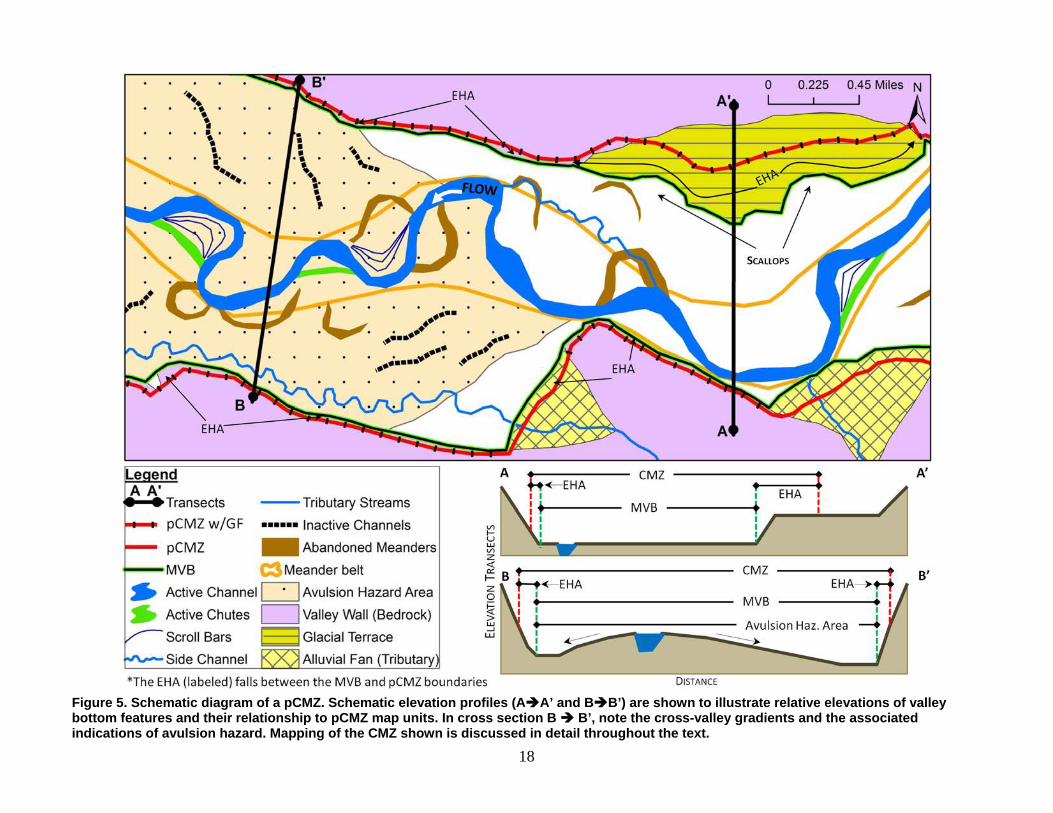
Figure 5. Schematic diagram of a pCMZ. Schematic elevation profiles (AA’ and BB’) are shown to illustrate relative elevations of valley bottom features and their relationship to pCMZ map units. In cross section B B’, note the cross-valley gradients and the associated indications of avulsion hazard. Mapping of the CMZ shown is discussed in detail throughout the text.

19

Modern Valley Bottom mapping (Data Sheet Section 2, Appendix A) The Modern Valley Bottom (MVB) defines the area where channel migration has occurred in the current climatic and hydrologic regime, which is assumed to encompass the last several thousand years. The boundary of the MVB encompasses fluvial landforms on the geomorphic surface where the current channel actively migrates (Figure 5). The MVB is, by definition, equal to or greater than areas occupied by the channel in the historical period. The MVB encompasses landscape features that record past channel migration, and indicate likely future channel migration activity. Over time, streams with a history of active migration are known to repeatedly reoccupy areas that they have in the past (O’Connor et al., 2003; Konrad, 2012). For this reason, the MVB will encompass areas likely to experience future channel migration. In this sense, the MVB uses past evidence of channel migration to predict a portion of the future influence of channel migration. Mapping of the MVB requires evaluating the extent of (1) soil survey map data, (2) geologic map data, and (3) valley bottom features and landforms indicating active channel migration. The MVB boundary is mapped to encompass the domain of active channel influence determined through multiple lines of evidence. Local soil survey reports are an essential guide to soils of floodplains and valley bottoms. Geologic maps also typically include younger units of alluvium (stream-lain sediment), which can provide an approximation for the MVB. Topography, landforms, and vegetation often reveal previous channel locations. The MVB boundary often will coincide with landform boundaries defining significant elevation breaks, such as stream terraces and intersections of valley bottoms and side slopes (Figure 5). Mapping of the MVB also includes an evaluation of possible aggradation (deposition) or incision (downward erosion) in the active channel. Aggradation and incision have potential to directly influence channel migration rates. Areas of active aggradation should be noted as areas with increased potential for migration. Alternatively, areas with active incision may have enhanced chances of channel bank collapse, a process that can affect adjacent infrastructure.

Soil survey map data Natural Resource Conservation Service (NRCS) soil information can provide great help with delineating the Modern Valley Bottom (O’Connor, 2001; Wallick et al., 2013). Key criteria in mapping and defining soil units are landform position and age, which influence soil type and development. As such, soil map units contain information about relative landform age and origin and, in turn, MVB extent. In general, soil information is used as an indicator of MVB extent, as opposed to a measure of landform erosion susceptibility. Local soil survey reports should be gathered in order to identify the key soil map units found in floodplains and valley bottoms. Also important are map units found on terraces or other features near the valley bottom that may be considered within the MVB. Soil survey reports often organize soil map units by landform and landscape position, which simplifies the task of identifying soil map units likely to be in or out of the MVB. While the characteristics of each local soil map unit should be considered, soil map units grouped under headings like “Soils on Floodplains and Terraces” or “Soils of Alluvial Floodplains” will often be within the MVB. Map

20

units grouped as “Soils on Older Terraces” will often fall outside of the MVB. Map units are also commonly grouped as “Soils on Younger Terraces.” The detailed descriptions of landforms considered as “younger terraces” will reveal whether they should be considered in the MVB. For example, the younger terraces discussed in the Soil Survey of Thurston County, Washington - an area shaped by the continental glaciers - are found on terraces composed of glacial outwash. Continental glaciers were present over 10,000 years before present, so soil map units on “younger terraces” should be excluded from the MVB in Thurston County. When mapping the CMZ, soil map units are ideally overlain on elevation data in a geospatial environment. Soil layers for GIS programs are available through the NRCS Web Soil Survey (http://websoilsurvey.sc.egov.usda.gov/). Landforms are then included or excluded from the MVB depending on their predominant soil map units. Because soil survey maps often were mapped many decades ago when high-resolution topography was not available, it is important that final MVB boundaries are delineated based soil survey data and topography in conjunction.

Geologic map data Geologic maps provide information about the age, composition, and extent of geological materials and landforms, which help delineate the Modern Valley Bottom. The common map unit of Quaternary alluvium (Qal) can be used as a preliminary indication of the MVB. In general, Quaternary alluvium is considered to have been deposited by the modern stream in a given valley. Geologic maps range in scale and content, which in turn influences the utility of geologic maps to pCMZ mapping. Publically available geological maps range in scale from 1:24,000 (termed Quadrangle maps) to covering entire states. Where ever available, large-scale 1:24,000 scale maps should be used. The most typical geological map is the bedrock map. Despite their main purpose to display the extent of bedrock geologic units, Quaternary alluvium is commonly mapped on bedrock maps. Surficial geologic maps, though less-widely available than bedrock maps, provide even greater division between units of Quaternary-age sediments than bedrock maps. Oftentimes, terraces of different ages within the Quaternary are mapped, or alluvial units originating from the Holocene (~11,000 years ago to present) and Pleistocene (greater than 11,000 years before present) are mapped separately. Geological maps are available from the U.S. Geological Survey Publications Warehouse (http://pubs.er.usgs.gov/), or from State geological agencies. In Washington, the Department of Natural Resources Division of Geology has a number of geological maps available online (http://www.dnr.wa.gov/researchscience/pages/pubmaps.aspx). The Washington State Department of Natural Resources also has Washington State GIS geology layers, including landslide layers, available for download (http://fortress.wa.gov/dnr/app1/dataweb/dmmatrix.html).

Valley bottom features and landforms A key step in mapping the Modern Valley Bottom is noting (and optionally mapping) features that indicate past and presently active channel migration (Figure 5). The MVB will encompass these features determined to have resulted from channel migration within the current climatic

21

and hydrologic regime. The analyst uses the presence or absence of features described below to determine whether channel migration has occurred. These features may be visible in topography, aerial images, or both. In general, if any of the below features are observed, the channel should be identified as an actively migrating stream. The last sub-section describes possible procedures for delineating the CMZ in unconfined valleys where none of the below features are observed.

Meander scrolls Meander scrolls are small-scale ridges formed on sediment bars located on the inside of meander bends that record the gradual migration of a meander bend (Leopold et al., 1995). Meander scrolls typically form roughly parallel to the active channel on the inside of meander bends, and may support vegetation and forests that increase in age with distance from the channel. Meander scrolls are visible in Panel D of Figure 4 and shown conceptually (scroll bars) in Figure 5.

Vegetation Migration is the process by which streams create and move away from an alluvial landform (usually a point bar) providing surfaces where vegetation (e.g., pioneer species, shrubs, trees) may subsequently germinate. Floodplain vegetation type, size and age may preserve a record of channel change through time (Sigafoos, 1964). In particular, trends of increasing size of vegetation with distance from the channel on the insides of meander bends indicate active channel migration. Forest canopy structure can also help identify the presence of active or recently abandoned side channels. The presence of recently established vegetation adjacent to the active channel may indicate an episode of channel widening followed by channel entrenchment and subsequent vegetation encroachment following a flood or series of floods. Vegetation characteristics can be assessed using aerial imagery and digital canopy models produced from LiDAR data. In areas where forests have been altered more recently than the channel has moved, forest age and structure will not provide reliable information on channel migration.

Channel width Variation of the active channel width is a simple indicator for migration activity along a channel, as found by Brice (1982) and confirmed by Lagasse et al. (2004). The active channel is defined as the wetted channel area plus the un-vegetated bars and surfaces adjacent to the wetted channel (Konrad et al., 2011). Active channels that vary from wide, near the outside of meander bends, to narrow at the inflection points between bends, generally migrate at greater rates than channels with equal width along their course (Brice, 1982). Sinuous streams with equal width and no exposed bars tend to migrate slowly, and are considered to be relatively stable (Brice, 1982).

Meander cutoffs and oxbow lakes Oxbow lakes and abandoned meanders visible in aerial imagery or LiDAR indicate active channel migration. The frequency at which meanders are “cut-off” is partially dependant on the rate of channel lengthening as a result of gradual bend migration (Constantine and Dunne, 2008). Cutoffs are classified as neck and chute cutoffs, and both result in the formation of abandoned meanders and oxbow lakes (Schumm, 1985) (shown in Figure 4 and Figure 5). Neck cutoffs occur when channel migration causes the channel to impinge upon itself, creating a new, straighter channel while at the same time the meander bend is abandoned (Figure 2). Neck cutoffs are most common in channels with high sinuosity where floodplain surfaces are resistant to scour and vertical erosion by overbank flows. Floodplains resistant to vertical erosion have

22

gentle floodplain gradients, heavy vegetation cover, and are composed of erosion-resistant material (Dunne et al., 2010). Chute cutoffs occur when a new channel is incised across a meander bend and a former meander is abandoned (Dunne et al., 2010) (Figure 2). Chute cutoffs tend to occur in actively migrating channels with relatively low sinuosity (Constantine and Dunne, 2008). Vegetation and other features can provide rough age estimates of cutoffs and oxbow lakes. Extent and structure (i.e. implied relative age) of nearby trees can also provide information on the relative age of abandoned meanders and oxbows. In cases where an oxbow lake is named on local maps, it is likely a relatively old and persistent feature on the valley bottom. Some abandoned meanders and oxbows are relics of past climatic and hydrologic regimes and thus are not within the MVB. For example, abandoned meanders and oxbows located on terraces deposited during the last glacial episode would be considered outside of the MVB. In these cases, soils and geologic information (discussed above) will help determine whether a given set of fluvial landforms should be considered within the MVB.

Vertical channel changes and channel migration Channels can actively aggrade (build their beds through channel deposition), which can drive channel migration. In general, aggrading channels often have enhanced migration rates because deposition of sediment as bars directs water toward the outside of meander bends and induces lateral erosion (Dunne et al., 2010). Aggradation of channel beds occurs naturally along particular stream reaches where reductions in channel slope make the channel unable to transport the sediment supplied to it (Montgomery and Buffington, 1997). Reaches of the channel with on-going aggradation often can be recognized due to their common landforms. Locations where the valley rapidly widens moving downstream often have accompanying reductions in gradient and aggradation. Stream channels also often form alluvial fans in locations where valleys widen and channel gradients lessen. Alluvial fans are fan-shaped landforms that form as a result of sediment deposition over time. Their apex occurs where a channel emerges from a narrow valley. Channels often switch and avulse on alluvial fans so they are also hazardous areas for development. Alluvial fans are discussed further in a dedicated section below. A channel may also aggrade in response to changes in sediment supply from its watershed. Changes in sediment supply can result from natural or human-induced disturbances. Natural disturbances such as landslides and debris flows can often induce channel aggradation in streams. Man-made disturbances often relate to changes in land use and forest practices (Montgomery, 1994). Channel aggradation is best observed using sequences of aerial photographs, which allow observation of channel change through time. Historical aerial photographs in Google Earth® - often extending back to the early 1990s – are usually the most readily available to observe recent aggradation. Aerial images should be used to identify bar formation in a channel. Sediment bars can build along channel banks or within the channel. It should also be noted that channel widening in response to large floods may create the appearance of newly deposited bars. Thus,

23

whenever possible, channel widening should be distinguished from aggradation. Areas with active aggradation or landforms indicating long-term aggradation (e.g. alluvial fans) should be flagged as potential high hazard areas. Alluvial fans are mapped as a separate map unit, as discussed in below. Stream channels can also incise, or lower their beds through erosion, in response to changes in their watersheds. Incision can result from channel modification such as straightening or dredging (Simon, 1989) or enhanced peak flows from land-use change, urbanization, or changing flood regimes in response to climate change (Konrad and Booth, 2002; Booth et al., 2004; Elsner et al., 2010). Incised channels tend to migrate less than they might otherwise. However, elevated banks often are unstable along incised streams, causing a predictable change that affects adjacent areas (Simon, 1989). In particular, incised streams tend to first incise, and then undercut their banks causing bank failure. Bank failure progresses until channels widen. Channel widening then induces aggradation of the channel. Channel incision is generally more difficult than aggradation to recognize using remotely-sensed data; however, common indications may include: • Steep banks and failures visible in LiDAR. • Un-naturally straight channels relative to reaches upstream and downstream (indicative of

channel straightening). • Extensive sediment faces observed along banks.

As with areas with aggradation, active incision should be flagged due to hazards adjacent to the channel.

Application: Modern Valley Bottom mapping in Figure 5 Figure 5 shows a hypothetical valley bottom with a pCMZ mapped. The MVB boundary, shown as a black and neon green line, is mapped along three different landform types, including: (1) the base of valley hillslopes composed of bedrock; (2) the base of tributary alluvial fans; and, (3) the base of Pleistocene-aged glacial terraces. The MVB in all cases encompasses the observed fluvial landforms such as cutoffs and meander scrolls present on the valley bottom. Where there is a lack of geologically recent landforms from the current climatic and hydrologic regime, the MVB boundary is mapped at intersections with the valley bottom and bedrock hillslopes. MVB boundaries placed at the base of tributary alluvial fans demarcate the boundary between portions of the valley influenced heavily by the tributary stream and the main channel of interest. Finally, MVB boundaries are mapped to exclude the Pleistocene-aged glacial terraces (greater than 11,000 years old), due to the known origin and age of the features falling outside of the current climatic and hydrologic regime.

Avulsion Hazard Area mapping (Data Sheet Section 3, Appendix A) Potential and existing Avulsion Hazard Areas are mapped as a sub-unit within the Modern Valley Bottom. Mapping Avulsion Hazard Areas notifies planners and pCMZ users of the potential for abrupt changes in channel course, which can have catastrophic consequences for adjacent property and infrastructure. In general, mapped Avulsion Hazard Areas identify areas susceptible to larger-scale avulsions (island-forming and regional avulsions in Figure 2), defined

24

here as those avulsions that roughly exceed the size of regular meander cutoffs. However, it also may be appropriate to map Avulsion Hazard Areas in the area within meander bends covering large areas of the floodplain. Avulsions occur when overbank flows from a main channel take advantage of and permanently occupy secondary or relict channels on the floodplain or create new floodplain channels (Slingerland and Smith, 2004). In addition, avulsions can also occur when man-made levees are breached and a channel takes advantage of low-lying areas behind the levee. Avulsions are hazardous in developed areas because they occur quickly, can cause substantial property damage, and endanger people. Conditions leading to avulsions are not always evident. Research shows that avulsion mechanisms are diverse and vary by stream and valley morphology, vegetation coverage, and geologic conditions (Abbe and Montgomery, 1996; Slingerland and Smith, 1998, 2004; Collins et al., 2003; Brummer et al., 2006; Tooth et al., 2007; Makaske et al., 2002; Collins and Montgomery, 2011; Collins et al., 2012) For example, large valley-scale avulsions (may be many miles in length) may occur along streams that form alluvial ridges, which are products of channel aggradation over many hundreds or thousands of years. In these cases, a steep cross-valley gradient between the alluvial ridge and the lower flood basin can lead to natural levee breaks and channel formation through the flood basin (Slingerland and Smith, 1998, 2004). Channel aggradation may also induce avulsions. Makaske et al. (2009) found that large avulsions in the Upper Columbia River occur because of channel bed aggradation inducing losses in channel capacity which caused relatively greater overbank flow. While the causes and timing of avulsions are often unpredictable, some conditions of note can indicate where avulsion potential exists. Slingerland and Smith (1998) found that avulsions tend to occur when the slope ratio (avulsion pathway slope to main channel slope) is high (greater than approximately 4). Tooth et al. (2007) reported that increases (2-3 times) in floodplain gradient in a downstream direction enhance the likelihood of avulsions. While these relative floodplain slope values should not be used as hard thresholds to predict avulsions, they provide a measure of valley bottom conditions that may lead to avulsions. In addition to variations in slope across and along a valley bottom, avulsion potential also likely relates to the resistance of the valley bottom surface to vertical erosion. Factors that influence erosion resistance include the nature and abundance of vegetation, and the composition and cohesion of floodplain sediments (Constantine et al., 2009; Dunne et al., 2010). Avulsion Hazard Areas may therefore be more likely in areas with sparse vegetation such as tilled agricultural fields than those with forests. Similarly, if the roughness of floodplains provided by vegetation is much less than channel roughness, overbank flows may have large erosive power on floodplains and induce avulsions (Wallace and Geyer, 2000). Large wood accumulations and channel-spanning logjams can also promote avulsions, but generally promote chute cutoff and island-forming avulsions (Figure 2) that occur as part of important natural floodplain processes (Abbe and Montgomery, 1996; Brummer et al., 2006; Collins et al., 2012, 2003). Because of the mobility of wood, the locations of avulsions induced

25

by large wood are difficult to delineate. However, in areas where large log jams are visible in the channel, delineation of Avulsion Hazard Areas may be warranted. While no exact rules define Avulsion Hazard Area delineation, the analyst should consider factors including: • Cross-valley gradients relative to main channel gradients (Figure 5). • Areas at lower elevations than the main channel with downstream outlets. • The presence of abandoned, side, or secondary channels that diverge from the active main

channel and have steeper slopes than the main channel (Figure 5). • The composition and cohesion of the floodplain and valley bottom sediments. • Abundance and type of vegetation in potential avulsion pathways. • Channels on an active alluvial fan or delta. • Indications of active channel aggradation or filling. • Accumulations of LWD and channel-spanning log-jams.

The analyst should use these features to map Avulsion Hazard Areas within the MVB. The MVB boundary must fall landward of the Avulsion Hazard Area.

Application: Avulsion Hazard Area mapping in Figure 5 An Avulsion Hazard Area is mapped on the west side of Figure 5. Key features that indicate avulsion hazards are (1) the floodplain surface that slopes toward the valley wall and away from the channel (as visible in cross section B), and (2) inactive channels (shown in black dashed lines on the map). The floodplain gradients from the channel toward the valley wall visible in valley cross section indicate that over-bank flood waters may have enhanced erosive power to either cut new channels across the floodplain or permanently occupy mapped inactive channels. The tributary stream entering from the south and running along the valley margin also indicates the presence of the cross-valley gradient and suggests the area along the valley wall could capture overbank flows from the main channel. As well as creating avulsion pathways, the inactive channels may suggest that partial avulsions have occurred in the past. The cross-valley gradients extend to the valley walls, so the Avulsion Hazard Area is mapped to the boundary of the MVB.

Erosion Hazard Area mapping (Data Sheet Section 3, Appendix A) The Erosion Hazard Area (EHA) – the second core component of the pCMZ - is an area added to the MVB to account for potential valley widening caused by future channel migration. The outer boundary of the EHA will define the boundary of the pCMZ. Where future migration has potential to impinge upon high ground and induce slope instability, Geotechnical Flags are mapped on the outer pCMZ boundary to indicate the geotechnical hazard potential. Because the outer boundaries of the EHA and pCMZ coincide, the Geotechnical Flag is mapped in conjunction with the EHA. Robust CMZ methods (Rapp and Abbe, 2003) include mapping of a Geotechnical Setback to account for the lateral influence of slope instability. However, mapping the Geotechnical Setback is optional for the pCMZ method. When the analyst elects to map a Geotechnical Setback, it is considered a sub-map unit of the EHA. This section describes methods and considerations for mapping the EHA, Geotechnical Flags, and Geotechnical Setbacks.

26

Valley history and the Erosion Hazard Area Valley form and widening depend largely on the geologic history of the stream and valley over geologic timescales. Over geologic time, the rate of valley widening depends on the stream power, the erodibility of the valley walls, and the tendency of a channel to migrate. In cases where a stream and valley have been in approximate steady-state form over geologic time, the size of the valley may reflect the balance between the channel’s lateral erosion potential and the valley wall’s resistance to erosion. In many cases, however, a stream in its current form is drastically different from the stream that carved its valley. Underfit streams represent one example where stream size does not scale with valley size (Dury, 1964, 1965). An underfit stream has a smaller discharge than the ancestral stream that carved the valley, which leads to no or relatively small valley widening rates at present. In many cases, the MVB will not extend to the physical valley walls for underfit streams. In other cases, the stream and valley may be actively forming or responding to some geomorphic disturbance causing either channel incision or aggradation resulting in valley expansion (Schumm,1993; Collins and Montgomery, 2011). Rates of lateral erosion along valley walls will likely be relatively high in these settings. Given these situations, geology and geologic history should be considered when mapping the EHA and the geotechnical sub-map units.

Determining the Erosion Hazard Area width While considerations of valley widening over time can provide a context to the Erosion Hazard Area (EHA) width determination, the EHA-width will largely depend on the current state and configuration of the channel and valley, and landform types along the valley (Figure 5). The EHA is analogous to the Erosion Hazard Zone of Rapp and Abbe (2003), but is mapped differently. The width of the Erosion Hazard Zone of detailed CMZ methods is determined by extrapolating measured rates of channel migration into the future while accounting for geological materials. Channel migration rates are not available for pCMZ delineations; therefore, EHA-widths are figured qualitatively given valley conditions. EHA widths are generally scaled to the size of the channel or meander belt. Factors considered in the EHA-width determination include: • Erodibility of Valley Margin: The resistance of the landforms at MVB boundary to future

lateral erosion depends on the characteristics of the valley wall. o Valley Wall Composition: Valley walls composed of bedrock will generally be

erosion resistant in the timescales considered for the pCMZ. On the other hand, valley margins composed of alluvium and glacio-fluvial sediments should be considered erodible (Figure 1). Glacially-derived till and other ice-contact deposits often have high-clay content making them relatively erosion resistant. In addition, glacial deposits often have large grain sizes that exceed the size of sediment the present day stream is able to transport. Glacially-derived till is considered to have intermediate erodibility. Geotechnical properties of local geologic materials and slope stability should also be considered.

o Valley Wall Height: In general, higher valley walls produce greater volumes of material for a given distance a channel erodes into a valley wall. Thus, landform height corresponds with the amount of sediment introduced to a stream for a given distance eroded, where a stream has to transport greater amounts of sediment on high landforms relative to low landforms. High landforms therefore should have greater

27

erosion resistance than lower ones. As discussed above, other factors such as erodibility and stability of valley wall geologic materials can affect this relationship.

• Channel Impingement on Valley Margin: Channel impingement and stream erosion along a valley wall depends on the MVB width and the distance between the active channel and the MVB boundary.

o MVB Width: The valley width relative to the meander belt width relates to the frequency at which the channel will impinge upon, and thus erode, the valley wall. A channel’s meander belt is the envelop that connects the outermost points of each meander bend (as shown in Figure 5).

o Distance of the active channel to the MVB boundary: As distance between the active channel and the MVB boundary increases, the likelihood of the channel impinging upon and eroding the landforms defining the MVB boundary is less likely in the near-term.

The factors above are plotted along the opposing axes in Figure 6 in order to evaluate approximate EHA-widths for each landform type along the MVB. In addition to these factors, the presence and size of scallops (arcuate indentations on the valley wall created by lateral channel erosion, Figure 5) on the MVB margin can indicate past lateral erosion of valley walls and may suggest high erodibility of material along valley margins. Scallop size can be used as an additional measure to scale the EHA-width.

Figure 6. Conceptual diagram on determining EHA-width. The user plots valley characteristics along each of the axes. Individual axis values such as “Valley Wall Composition” and “Height-Scale of Valley Wall” are qualitatively combined to determine the overall rating for the axis (e.g.“Valley Margin Erodibility”), and in turn determine the Erosion Hazard Width in terms of channel and meander belt width. Actual widths can be adjusted to the local geological materials, but in general, are scaled to the size of the channel and meander belt. The meander belt is the envelope connecting locally extreme bends of the channel, as shown in Figure 5.

28

Application: Erosion Hazard Area mapping in Figure 5 The Erosion Hazard Areas shown in Figure 5 generally were determined qualitatively using concepts shown in Figure 6. Erosion Hazard Area widths were determined separately for each landform along the Modern Valley Bottom boundary. These landforms are (1) valley walls (bedrock), (2) the upstream-most tributary alluvial fan, (3) the downstream-most tributary alluvial fan, and (4) the Pleistocene-aged glacial terrace on the northern valley wall.

Bedrock valley walls Because the bedrock composing valley walls is generally volcanic in nature and relatively erosion resistant, EHA widths were all less than a channel width. The relatively large valley width relative to the active meander belt as well as the fact the active channel does not impinge upon valley walls further supported an EHA width of less than a channel width.

Tributary alluvial fans The two tributary alluvial fans were generally considered separately for EHA mapping, although a few common considerations applied. The fans, composed of erodible alluvium, are actively being built by their parent tributary streams. Sediment deposition by the tributary streams acts to push the main channel away, so the EHA widths are somewhat less than would be mapped on alluvial landforms without an active tributary stream. However, diversion of the main channel by tributary streams does not necessarily occur at all stream junctions. When mapping the EHA at tributary junctions, possible considerations may include: • The size of the tributary stream relative to the main channel. • Any visible indications the tributary stream is affecting the main channel (e.g. sediment

deposition at confluences) (Benda et al., 2004). • Visible indications that the main channel is eroding the alluvial fan. Of the two tributary alluvial fans in Figure 5, the one upstream has the greater EHA. This is due to its proximity and orientation relative to the active main channel. The tributary alluvial fan downstream is sheltered by a small bedrock landform, so the EHA width is small relative to the channel (less than one channel width).

Glacial terrace The glacial terrace on the north side of the valley is the most erodible of the landforms along the MVB. The presence of scallops along its outer edge indicates its susceptibility to lateral erosion. Scallops indicate the main channel has eroded laterally into the terrace in the past. The EHA was set to approximately one-half to one meander belt width, which was approximately the size of the valley scallops. The distance of the active meander belt from the terrace also suggested erosion would not impact the landform for some time. Alternatively, if the active channel was near or actively eroding the terrace, the EHA would have been mapped to a width greater than the meander belt.

Geotechnical Flags Channel migration can undermine high landforms and induce slope failure. The outer boundary of the EHA and pCMZ (which coincide) should be flagged where these hazards exist. Geotechnical Flags differ from most map units discussed to this point in that they do not represent an area within the pCMZ. Rather, Geotechnical Flags are notations added along the

29

pCMZ boundary where there is potential for slope instability induced by channel migration. Geotechnical Flags are added when landforms at the margins of the CMZ are high enough that slope failure would have a significant lateral influence. Figures 5 and 7 show the use of Geotechnical Flags. In general, Geotechnical Flags denote a potential hazard. They also identify areas where detailed geotechnical studies by professional geologists and engineers may be required if development is proposed along valley side slopes. The geologic composition and geotechnical properties of landforms along the valley margin should also be considered. For instance, high landforms composed of unconsolidated sediment such as shown in Figure 1 are more susceptible to failure than those composed of erosion resistant bedrock. While this document defines no specific landform-height threshold above which a Geotechnical Flag must be mapped, the analyst should consider the approximate lateral influence of potential slope failure relative to the precision of the pCMZ delineation. For landforms below approximately 25 feet, the lateral influence of potential slope failure is likely insignificant relative to the detail-level of pCMZ delineation. Geotechnical Flags may not be required in these scenarios. Existing landslides along valley margins can also be noted or mapped. The Washington State Department of Natural Resources has readily available geologic and landslide maps. Existing landslides are hazardous both for their immediate damages, and for their ability to divert and block stream channels. Landslides along narrow valleys particularly have the ability to alter the course and character of channels.

Application: Geotechnical Flags mapping in Figure 5 In Figure 5, Geotechnical Flags (indicated by black hash marks on red CMZ boundary) are mapped along any high landform at the CMZ boundary. These landforms include the valley walls (bedrock) and the glacial terrace. Note that relative geotechnical hazards are not denoted with geotechnical flags. Rather, the simple presence of a geotechnical hazards is flagged. Geotechnical Flags are not mapped on alluvial fans (in Figure 5) due to their minor height above the MVB surface elevation.

Geotechnical Setbacks (Optional) Where geotechnical hazards exist, a Geotechnical Setback can also be added as a sub-map unit to the EHA (sensu Rapp and Abbe, 2003). The Geotechnical Setback should be a standard practice for detailed CMZ delineations, but is optional for the pCMZ. If delineated in the pCMZ, the Geotechnical Setback is added to the original EHA-width described above (see Figure 7). In detailed CMZ methods, the Geotechnical Setback is quantitatively figured as the approximate lateral influence of potential slope failure induced by lateral erosion of a high landform. Detailed-CMZ methods of Rapp and Abbe (2003) provide a means of estimating a Geotechnical Setback using the vertical height (H, Figure 7) of the landform and an assumed (or measured) failure angle (θ):

𝐺𝑒𝑜𝑡𝑒𝑐ℎ𝑛𝑖𝑐𝑎𝑙 𝑆𝑒𝑡𝑏𝑎𝑐𝑘 =𝐻

tan(𝜃)

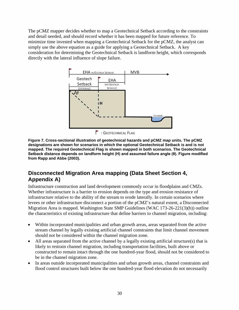
30

The pCMZ mapper decides whether to map a Geotechnical Setback according to the constraints and detail needed, and should record whether it has been mapped for future reference. To minimize time invested when mapping a Geotechnical Setback for the pCMZ, the analyst can simply use the above equation as a guide for applying a Geotechnical Setback. A key consideration for determining the Geotechnical Setback is landform height, which corresponds directly with the lateral influence of slope failure.

Figure 7. Cross-sectional illustration of geotechnical hazards and pCMZ map units. The pCMZ designations are shown for scenarios in which the optional Geotechnical Setback is and is not mapped. The required Geotechnical Flag is shown mapped in both scenarios. The Geotechnical Setback distance depends on landform height (H) and assumed failure angle (θ). Figure modified from Rapp and Abbe (2003).

Disconnected Migration Area mapping (Data Sheet Section 4, Appendix A) Infrastructure construction and land development commonly occur in floodplains and CMZs. Whether infrastructure is a barrier to erosion depends on the type and erosion resistance of infrastructure relative to the ability of the stream to erode laterally. In certain scenarios where levees or other infrastructure disconnect a portion of the pCMZ’s natural extent, a Disconnected Migration Area is mapped. Washington State SMP Guidelines (WAC 173-26-221(3)(b)) outline the characteristics of existing infrastructure that define barriers to channel migration, including: • Within incorporated municipalities and urban growth areas, areas separated from the active

stream channel by legally existing artificial channel constraints that limit channel movement should not be considered within the channel migration zone.

• All areas separated from the active channel by a legally existing artificial structure(s) that is likely to restrain channel migration, including transportation facilities, built above or constructed to remain intact through the one hundred-year flood, should not be considered to be in the channel migration zone.

• In areas outside incorporated municipalities and urban growth areas, channel constraints and flood control structures built below the one hundred-year flood elevation do not necessarily

31

restrict channel migration and should not be considered to limit the channel migration zone unless demonstrated otherwise using scientific and technical information.

In addition, all structures considered to be barriers to CMZs must also be legally existing structures. Legally existing structures are defined under the Shoreline Management Act definition for floodway (RCW 90.58.030) as those “...flood control devices maintained by or maintained under license from the federal government, the state, or a political subdivision of the state.” Only structures with a public agency commitment for maintenance are considered a barrier to channel migration. The pCMZ method uses existing geospatial data to identify barriers to migration, which include US Army Corps of Engineers-certified levees, state highways, active railroads and major county roads that provide sole access to infrastructure or habitations. Whenever possible, local databases of levee age and construction type should be consulted while delineating the pCMZ and Disconnected Migration Areas. Where levee databases are not available, knowledge and information on levees from local officials should be gathered by the mapping analyst. Areas within the pCMZ landward of structures determined as channel migration barriers are mapped as Disconnected Migration Areas. Channel migration is a primary process that creates and maintains floodplain habitats, so mapping of Disconnected Migration Areas provides an inventory of areas with potential for floodplain restoration. The utility of the pCMZ as a restoration planning tool depends on the detail and quality of data used to define Disconnected Migration Areas.

Mapping of other units (Data Sheet Section 4, Appendix A) The pCMZ method also includes optional units map units which denote unique types of hazard. The Potential Inundation Zone delineates areas on the floodplain or valley lower than the channel elevation, but outside the CMZ. Alluvial fans formed by tributary streams are also mapped to delineate hazardous areas with potential for channel avulsions. Due to their common association with tributary streams, alluvial fans can be mapped outside of the CMZ. In Washington State, a CMZ is delineated for shoreline streams (defined by the SMA) flowing on alluvial fans. CMZs can be mapped on non-shoreline stream alluvial fans for to bring attention to hazards.

Potential Inundation Zones A Potential Inundation Zone identifies low areas in the floodplain that have potential to be inundated during flooding. Potential Inundation Zones are only mapped outside of the pCMZ to denote flood inundation hazards extending landward of the pCMZ boundary. Potential Inundation Zones are common in valleys with underfit streams, where the MVB is narrower than the physical valley bottom. A Potential Inundation Zone may also be mapped in closed depressions with no outlet along irregular valley walls where Avulsion Hazard Areas are not appropriate. pCMZ versus FEMA Floodplain The boundaries of the CMZ and FEMA floodplain generally will not coincide, and should be considered independent of one another. Where a Potential Inundation Zone is mapped, the FEMA floodplain will likely exceed the width of the CMZ. FEMA floodplains will commonly

32

exceed the CMZ in underfit streams with low gradients and little migration potential (shown in left panel in Figure 8). Alternatively, CMZs may exceed the FEMA floodplain in actively migrating streams. CMZs mapped outside FEMA floodplain boundaries are common where erodible terraces at the FEMA floodplain boundary are contained within the CMZ (shown in right panel in Figure 8).

Figure 8. CMZs versus FEMA floodplains. Schematic illustrations of valleys where the FEMA floodplain (orange) is wider than the CMZ (left), and the CMZ (red) is larger than the FEMA floodplain (right). The stream in the left panel is underfit, as indicated by the Quaternary glacial outwash (Qg) composing the valley floor. The stream on the right has incised (cut into) a deposit of Quaternary alluvium (Qa) susceptible to lateral channel erosion.

Alluvial fans Alluvial fans often form along the edges of larger valleys at the mouths of tributary valleys (Bull, 1977). Alluvial fans develop over time as a stream deposits sediment at abrupt reductions in channel gradient and sediment transport capacity. Sporadic switching of the parent channel forms a convex, fan-shaped landform. The natural tendency for channels to avulse on alluvial fan surfaces makes them hazardous areas. The alluvial fan map unit provides extra hazard information to the CMZ user, but does not replace any of the pCMZ map units. The alluvial fan should therefore be mapped in addition to other pCMZ map units. Alluvial fans should be mapped using a separate map unit when either the subject stream has deposited the alluvial fan, or when tributary streams have deposited alluvial fans in the valley bottom of the pCMZ stream. In the case where the subject stream of the pCMZ mapping has deposited an alluvial fan, the pCMZ will generally encompass the entire alluvial fan landform unless the analyst determines that the alluvial fan is a product of a past climate and is presently abandoned. Avulsion Hazard Areas are a common unit within alluvial fans deposited by the pCMZ stream. Mapped alluvial fans formed by tributary streams will often extend outside of the pCMZ boundaries, but are necessarily mapped to show hazards.

Planning-Level CMZ mapping in unconfined valleys with minimal migration In some valleys where valley width is large relative to the stream, and indications of channel migration are minimal, alternatives to the main pCMZ approach described above may be warranted. These scenarios are most prevalent with underfit streams flowing through valleys

33

eroded during a past climate when the parent stream was much larger and erosive. These streams should be identified using the following criteria: • The present-day stream must have no indications of active channel migration as discussed in

the section on MVB mapping (above). Note that a stream may be sinuous and have no indications of active channel migration.

• The present-day stream must be deemed underfit (Dury, 1964), based on a known geologic history of a valley indicating a drastic reduction in stream discharge and/or erosive power. Common causes for underfit streams in Washington include past carving of valleys by large glaciers or glacial streams draining ice sheets. Present-day streams occupying these valleys have drastically less erosive power than the original stream or glacier.

• The physical valley bottom is too large to reasonably be considered the MVB. If a stream meets the criteria above, an alternative pCMZ mapping approach includes: • The pCMZ boundaries are mapped approximately one meander belt width on either side of

the channel’s present-day meander belt. A channel’s meander belt is the envelop that connects the outermost points of locally extreme meander bends (as shown in Figure 5). Therefore, the pCMZ will be approximately three meander belt widths wide. The meander belt would encompass the area affected by a cycle of meander bend migration and cutoff, if it were to occur in the future.

• The MVB map unit is not mapped. In valleys containing underfit streams, there oftentimes are no landforms within the physical valley bottom on which to map the MVB. Therefore, the MVB is not mapped in order to avoid arbitrary map unit delineation.

The Goldsborough Creek example in Appendix B is an underfit stream in which an approach similar to this was used.

Recommended QA/QC review The following process is recommended for QA/QC review. Senior-level geomorphologists should review delineations in conjunction with reach-data sheets. Each QA/QC reviewer should evaluate the channel migration maps and data sheets individually and recommend any changes, if necessary. Then the mapping analysts and reviewers should meet as a group and discuss the draft maps and the recommendations changes.

Method limitations The pCMZ methodology is a conservative assessment that uses remotely-sensed data as a basis for delineating areas of potential channel migration. The planning-level method does not analyze historical channel occupation or migration rates, and therefore does not allow for assignment of a CMZ design life (effective time period). As a result, the pCMZ boundary line is a conservative approximation of areas reasonably likely to be influenced by channel migration. While channel migration should be considered unlikely outside of the CMZ boundary, extreme events where channel migration occurs outside of CMZ boundaries are nonetheless possible. Where and when a perceived threat to infrastructure or life is present, a detailed-level assessment should be undertaken to quantify channel migration rates and processes. These methods are provided as guidance. The responsibility for pCMZ map quality falls solely upon the practitioner applying

34

the pCMZ method. As such, the method outlined above should be considered a conceptual framework, but not a prescription, for pCMZ mapping.

35

References Cited Abbe, T.B., and Montgomery, D.R., 1996, Large woody debris jams, channel hydraulics and

habitat formation in large rivers: Regulated Rivers Research & Management, v. 12, p. 201–221.

Beechie, T., and Bolton, S., 1999, An approach to restoring salmonid habitat-forming processes in Pacific Northwest watersheds: Fisheries, v. 24, p. 6–15.

Benda, L., Poff, N.L., Miller, D., Dunne, T., Reeves, G., Pess, G., and Pollock, M., 2004, The network dynamics hypothesis: how channel networks structure riverine habitats: BioScience, v. 54, p. 413–427.

Booth, D.B., Karr, J.R., Schauman, S., Konrad, C.P., Morley, S.A., Larson, M.G., and Burges, S.J., 2004, Reviving Urban Streams: Land Use, Hydrology, Biology, and Human Behavior: JAWRA Journal of the American Water Resources Association, v. 40, p. 1351–1364.

Brice, J.C., 1982, Stream channel stability assessment: Federal Highway Administration FHWA/RD-82/021, 48 p.

Brooks, A.P., and Brierley, G.J., 2002, Mediated equilibrium: the influence of riparian vegetation and wood on the long-term evolution and behaviour of a near-pristine river: Earth Surface Processes and Landforms, v. 27, p. 343–367.

Brooks, A.P., Brierley, G.J., and Millar, R.G., 2003, The long-term control of vegetation and woody debris on channel and flood-plain evolution: insights from a paired catchment study in southeastern Australia: Geomorphology, v. 51, p. 7–29.

Brummer, C.J., Abbe, T.B., Sampson, J.R., and Montgomery, D.R., 2006, Influence of vertical channel change associated with wood accumulations on delineating channel migration zones, Washington, USA: Geomorphology, v. 80, p. 295–309, doi: 10.1016/j.geomorph.2006.03.002.

Bull, W.B., 1977, The alluvial-fan environment: Progress in Physical Geography, v. 1, p. 222–270.

Collins, B.D., and Montgomery, D.R., 2011, The legacy of Pleistocene glaciation and the organization of lowland alluvial process domains in the Puget Sound region: Geomorphology, v. 126, p. 174–185.

Collins, B.D., Montgomery, D.R., Fetherston, K.L., and Abbe, T.B., 2012, The floodplain large-wood cycle hypothesis: A mechanism for the physical and biotic structuring of temperate forested alluvial valleys in the North Pacific coastal ecoregion: Geomorphology, v. 139-140, p. 460–470, doi: 10.1016/j.geomorph.2011.11.011.

36

Collins, B.D., Montgomery, D.R., and Sheikh, A.J., 2003, Reconstructing the historical riverine landscape of the Puget lowland: Restoration of Puget Sound Rivers. University of Washington Press, Seattle, WA,, p. 79–128.

Constantine, J.A., and Dunne, T., 2008, Meander cutoff and the controls on the production of oxbow lakes: Geology, v. 36, p. 23.

Constantine, J.A., McLean, S.R., and Dunne, T., 2009, A mechanism of chute cutoff along large meandering rivers with uniform floodplain topography: Geological Society of America Bulletin, v. 122, p. 855–869.

Dunne, T., Constantine, J.A., and Singer, M.B., 2010, The Role of Sediment Transport and Sediment Supply in the Evolution of River Channel and Floodplain Complexity: Transactions, Japanese Geomorphological Union, v. 31, p. 155–170.

Dury, G.H., 1964, Principles of underfit streams: US Government Printing Office.

Dury, G.H., 1965, Theoretical implications of underfit streams: US Government Printing Office.

Eaton, B.C., 2006, Bank stability analysis for regime models of vegetated gravel bed rivers: Earth Surface Processes and Landforms, v. 31, p. 1438–1444.

Elsner, M.M., Cuo, L., Voisin, N., Deems, J.S., Hamlet, A.F., Vano, J.A., Mickelson, K.E.B., Lee, S.-Y., and Lettenmaier, D.P., 2010, Implications of 21st century climate change for the hydrology of Washington State: Climatic Change, v. 102, p. 225–260, doi: 10.1007/s10584-010-9855-0.

FEMA (Federal Emergency Management Agency), 2010, Draft Model Ordinance for Floodplain Management under the National Flood Insurance Program and the Endangered Species Act Produced by FEMA - Region 10 July 2010, Bothell, WA 98021-9796

Fetherston, K.L., Naiman, R.J., and Bilby, R.E., 1995, Large woody debris, physical process, and riparian forest development in montane river networks of the Pacific Northwest: Geomorphology, v. 13, p. 133–144.

Florsheim, J.L., Mount, J.F., and Chin, A., 2008, Bank erosion as a desirable attribute of rivers: BioScience, v. 58, p. 519–529.

Hooke, R.L.B., 1967, Processes on arid-region alluvial fans: The Journal of Geology,, p. 438–460.

Jones, J.L., 2006, Side channel mapping and fish habitat suitability analysis using lidar topography and orthophotography: Photogrammetric engineering and remote sensing, v. 72, p. 1202.

Jones, J.A., and Grant, G.E., 1996, Peak flow responses to clear-cutting and roads in small and large basins, western Cascades, Oregon: Water Resources Research, v. 32, p. 959–974.

37

Knighton, D., 1998, Fluvial forms and processes: a new perspective.: Arnold, Hodder Headline, PLC.

Konrad, C.P., 2012, Reoccupation of floodplains by rivers and its relation to the age structure of floodplain vegetation: Journal of Geophysical Research, v. 117, doi: 10.1029/2011JG001906.

Konrad, C., Berge, H., Fuerstenberg, R., Steff, K., Olsen, T., and Guyenet, J., 2011, Channel Dynamics in the Middle Green River, Washington, from 1936 to 2002: Northwest Science, v. 85, p. 1–14, doi: 10.3955/046.085.0101.

Konrad, C.P., and Booth, D.B., 2002, Hydrologic trends associated with urban development for selected streams in the Puget Sound Basin, western Washington: US Geological Survey.

Lagasse, P.F., Zevenbergen, L.W., Spitz, W.J., and Thorne, C.R., 2004, Methodology for predicting channel migration: Transportation Research Board, National Research Council.

Leopold, L.B., and Wolman, M.G., 1960, River Meanders: Geological Society of America Bulletin, v. 71, p. 769.

Leopold, L.B., Wolman, M.G., and Miller, J.P., 1995, Fluvial processes in geomorphology: Courier Dover Publications.

Makaske, B., Smith, D.G., and Berendsen, H.J., 2002, Avulsions, channel evolution and floodplain sedimentation rates of the anastomosing upper Columbia River, British Columbia, Canada: Sedimentology, v. 49, p. 1049–1071.

Makaske, B., Smith, D.G., Berendsen, H.J., de Boer, A.G., van Nielen-Kiezebrink, M.F., and Locking, T., 2009, Hydraulic and sedimentary processes causing anastomosing morphology of the upper Columbia River, British Columbia, Canada: Geomorphology, v. 111, p. 194–205.

Montgomery, D.R., 1994, Road surface drainage, channel initiation, and slope instability: Water Resources Research, v. 30, p. 1925–1932.

Montgomery, D.R., and Buffington, J.M., 1997, Channel-reach morphology in mountain drainage basins: Geological Society of America Bulletin, v. 109, p. 596.

Nanson, G.C., and Beach, H.F., 1977, Forest succession and sedimentation on a meandering-river floodplain, northeast British Columbia, Canada: Journal of Biogeography,, p. 229–251.

Nanson, G.C., and Croke, J.C., 1992, A genetic classification of floodplains: Geomorphology, v. 4, p. 459–486.

NMFS (National Marine Fisheries Service), 2008, Endangered Species Act – Section 7 Consultation Final Biological Opinion and Magnuson-Stevens Fishery Conservation and

38

Management Act, Essential Fish Habitat Consultation Implementation of the National Flood Insurance Program in the State of Washington Phase One Document – Puget Sound Region Lead Action Agency: Federal Emergency Management Agency Consultation. National Marine Fisheries Service Northwest Region Date Issued: September 22, 2008

O’Connor, J.E., 2001, Origin, extent, and thickness of Quaternary geologic units in the Willamette Valley, Oregon: US Geological Survey.

O’Connor, J.E., Jones, M.A., and Haluska, T.L., 2003, Flood plain and channel dynamics of the Quinault and Queets Rivers, Washington, USA: Geomorphology, v. 51, p. 31–59.

Olson, P.L, 2008, Web Guidance for Channel Migration Assessment under SMA, Washington Department of Ecology Publication 08-06-013, Olympia WA http://www.ecy.wa.gov/biblio/0806013.html http://www.ecy.wa.gov/programs/sea/sma/cma/index.html

Olson, P.L and J. Franklin , 2012, Quality Assurance Project Plan for Channel Migration Assessments of Puget Sound SMA Streams, Washington State Department of Ecology publication 12-06-006, https://fortress.wa.gov/ecy/publications/SummaryPages/1206006.html

Piégay, H., Darby, S.E., Mosselman, E., and Surian, N., 2005, A review of techniques available for delimiting the erodible river corridor: a sustainable approach to managing bank erosion: River Research and Applications, v. 21, p. 773–789, doi: 10.1002/rra.881.

Pittman, P.D., and Maudlin, M.R., 2003, Evidence of a major late Holocene river avulsion, in Abstracts with Programs, Seattle, Washington.

Rapp, C.F., and Abbe, T.B., 2003, A framework for delineating channel migration zones: Washington Department of Ecology Publication 03-06-027.

Schumm, S.A., 1985, Patterns of alluvial rivers: Annual Review of Earth and Planetary Sciences, v. 13, p. 5.

Schumm, S.A., 1993, River response to baselevel change: implications for sequence stratigraphy: The Journal of Geology,, p. 279–294.

Sigafoos, R.S., 1964, Botanical evidence of floods and flood-plain deposition: US Govt. Print. Off.

Simon, A., 1989, A model of channel response in disturbed alluvial channels: Earth Surface Processes and Landforms, v. 14, p. 11–26.

Skidmore, P., Cooper, P., and Boyd, K., 1999, Methodology for Determining Meander Corridor Limits: American Water Resources Association Watershed Management to Protect Declining Species, 4 p.

39

Slingerland, R., and Smith, N.D., 1998, Necessary conditions for a meandering-river avulsion: Geology, v. 26, p. 435, doi: 10.1130/0091-7613(1998)026<0435:NCFAMR>2.3.CO;2.

Slingerland, R., and Smith, N.D., 2004, River Avulsions and their Deposits: Annual Review of Earth and Planetary Sciences, v. 32, p. 257–285.

Tooth, S., Rodnight, H., Duller, G.A.T., McCarthy, T.S., Marren, P.M., and Brandt, D., 2007, Chronology and controls of avulsion along a mixed bedrock-alluvial river: Geological Society of America Bulletin, v. 119, p. 452–461, doi: 10.1130/B26032.1.

Wallace, D.C., and Geyer, W.A., 2000, Waterbreaks: Managed trees for the floodplain: Agroforestry Notes (USDA-NAC),, p. 19.

Wallick, J.R., Krista Jones, O’Connor, J.E., Keith, M.K., Hulse, D., and Gregory, S.V., 2013, Geomorphic and Vegetation Processes of the Willamette River Floodplain, Oregon--Current Undrstanding and Unanswered Questions: U.S. Geological Survey Open File Report 2013-1246, 70 p.

Ward, J.V., and Stanford, J.A., 1995a, Ecological connectivity in alluvial river ecosystems and its disruption by flow regulation: Regulated Rivers: Research & Management, v. 11, p. 105–119, doi: 10.1002/rrr.3450110109.

Ward, J.V., and Stanford, J.A., 1995b, The serial discontinuity concept: extending the model to floodplain rivers: Regulated Rivers: Research & Management, v. 10, p. 159–168.

Ward, J.V., Tockner, K., and Schiemer, F., 1999, Biodiversity of floodplain river ecosystems: ecotones and connectivity1: Regulated Rivers: Research & Management, v. 15, p. 125–139.

40

Appendices

41

Appendix A. Reach Datasheet

A Microsoft Excel version of the data sheet is available as a supplemental file online.

42

Appendix B. Example Planning-Level CMZ Delineations Contained in this appendix are five examples of planning-level CMZ (pCMZ) delineations. With each example are maps and supporting discussion of key considerations involved in delineating each example pCMZ. The examples include a variety of pCMZ scenarios and considerations on the following streams:

1. Middle Fork of the Nooksack River (Whatcom County): A relatively straight-forward pCMZ where fluvial landforms extend to the margins of the Modern Valley Bottom (MVB).

2. Bogachiel and Sol Duc Rivers (Clallam County): An underfit stream incised into glacially-derived deposits.

3. Elwha River (Clallam County): The CMZ encompasses high glacial-terraces actively being eroded by the stream.

4. Nisqually River (Pierce County): The MVB encompasses high landforms composed of volcanic mudflow (lahar) deposits.

5. Goldsborough Creek (Mason County): An underfit stream where the MVB boundary falls inside of the physical valley bottom.

Map units include boundaries of the Modern Valley Bottom (MVB) in green with black borders and the planning level CMZ (pCMZ) in red. Other map units used are identified specifically in each example.

43

Middle Fork Nooksack River (48°49'12.22" N 122°08'04.66" W)

This Middle Fork Nooksack reach is an anabranching channel subject to active migration and frequent small to large-scale avulsions. The LiDAR relative elevation model (REM, left image above) shows that repeated small and large scale channel avulsions occurred in the lower half of image over the last 100 years. The avulsion channels are also visible on the orthophoto image (right image above). Avulsion extent was controlled by continental sedimentary bedrock (Ec(cb) on left valley wall and M.F. Nooksack lahar deposits (Qvl(m)), glacial terraces, and alluvial fans (Qaf) on valley right. The downstream channel (upper part of image) is confined between lahar deposits on valley left and landslide and alluvial fan deposits on valley right. The MVB (green line with black border) mostly extends along the perimeters of both bedrock valley wall and the margins of glacial terraces (glacial and lahar deposits) and alluvial fans. The Erosion Hazard Area width (EHA) (area between the MVB and pCMZ boundary, red line) width is based on active channel widths. The EHA also includes abandoned and secondary channels as avulsion hazard areas. The EHA width is modified based on the erosion potential of the geologic units adjacent to the MVB. In general, the EHA is narrower along the bedrock valley wall where erosion potential is low and much wider along the glacial terrace where erosion potential is higher.

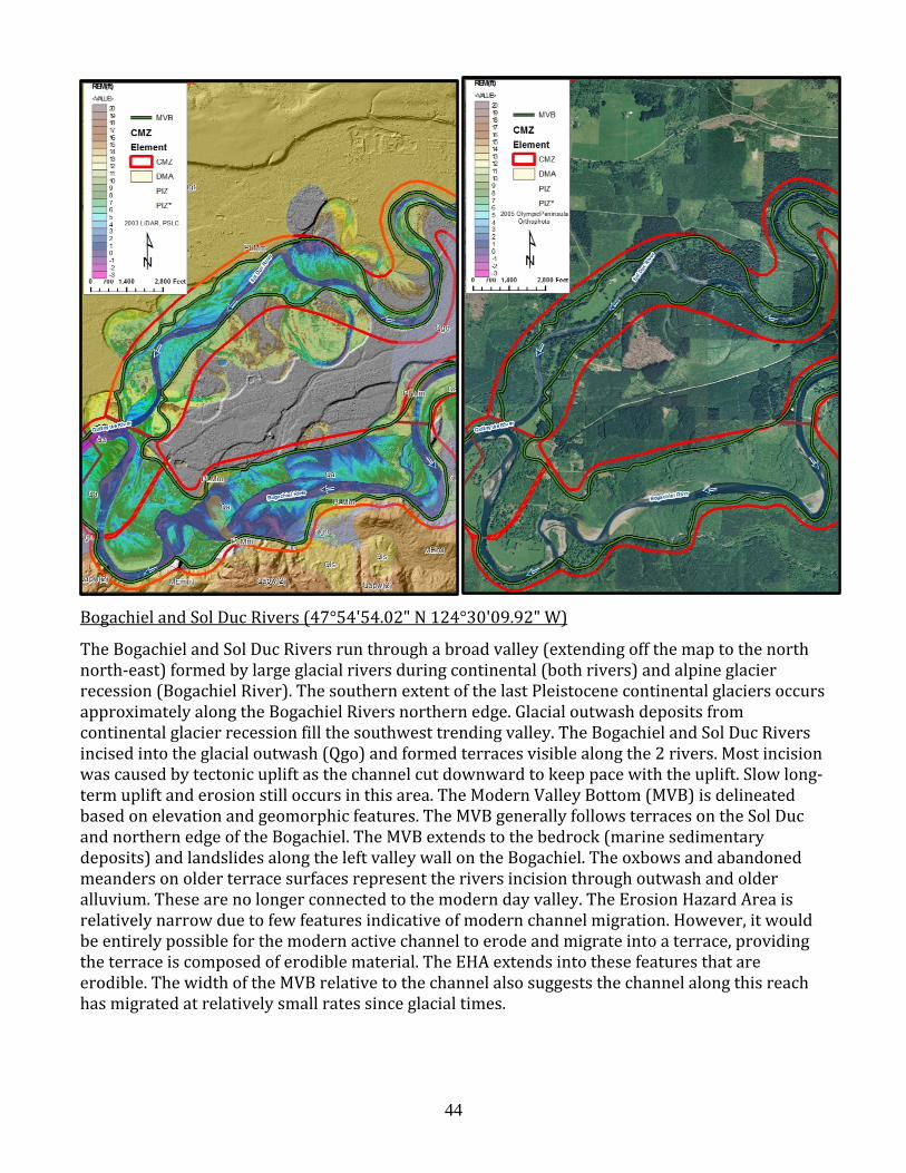
44

Bogachiel and Sol Duc Rivers (47°54'54.02" N 124°30'09.92" W)

The Bogachiel and Sol Duc Rivers run through a broad valley (extending off the map to the north north-east) formed by large glacial rivers during continental (both rivers) and alpine glacier recession (Bogachiel River). The southern extent of the last Pleistocene continental glaciers occurs approximately along the Bogachiel Rivers northern edge. Glacial outwash deposits from continental glacier recession fill the southwest trending valley. The Bogachiel and Sol Duc Rivers incised into the glacial outwash (Qgo) and formed terraces visible along the 2 rivers. Most incision was caused by tectonic uplift as the channel cut downward to keep pace with the uplift. Slow long-term uplift and erosion still occurs in this area. The Modern Valley Bottom (MVB) is delineated based on elevation and geomorphic features. The MVB generally follows terraces on the Sol Duc and northern edge of the Bogachiel. The MVB extends to the bedrock (marine sedimentary deposits) and landslides along the left valley wall on the Bogachiel. The oxbows and abandoned meanders on older terrace surfaces represent the rivers incision through outwash and older alluvium. These are no longer connected to the modern day valley. The Erosion Hazard Area is relatively narrow due to few features indicative of modern channel migration. However, it would be entirely possible for the modern active channel to erode and migrate into a terrace, providing the terrace is composed of erodible material. The EHA extends into these features that are erodible. The width of the MVB relative to the channel also suggests the channel along this reach has migrated at relatively small rates since glacial times.

45

Elwha River (48°07'33.16" N 123°33'12.12" W)

This reach of the Elwha River is anabranching and located just upstream of the river’s confluence with the Straits of San Juan de Fuca (Puget Sound). The reach flows along a 125-foot (41 m) high glacial outwash terrace on valley left. This geologic deposit is highly erodible. In places, the river channel is actively eroding the terrace and widening its valley. See photo insert as well as Figure 1.1 in the main body of the text. As a result, the pCMZ designates an Erosion Hazard Area that extends approximately one meander amplitude back from the edge of the high terrace. The width of this EHA can be refined in a more detailed CMZ analysis. A Geotechnical Flag should be mapped along the valley left CMZ shown. In the image, note the sediment that has accumulated at the base of the slope as a result of chronic instability.

The CMZ on valley right is constrained by a 100-year levee built and maintained by the US Army Corps of Engineers. The levee meets the criteria for a legal barrier to channel migration under Washington State Shoreline Management Act and Shoreline Master Programs. East of the levee to the MVB boundary is a disconnected migration area. However, two upstream dams are being removed and much sediment is being deposited in this reach. The CMZ boundary may need to be remapped in the near future.

46

Nisqually River (46°44'39.03" N 121°57'07.49" W)

The reach of the Nisqually River shown is a scenario where high landforms are within the Modern Valley Bottom (green line with black border). The gray areas marked >-5 feet are portions of the MVB that are more than -5.0 feet below the main channel. The landform outlined in white dotted line is a volcanic lahar deposit (large mudflow) originating from Mount Rainier. The most recent lahars that traveled down the Nisqually drainage occurred approximately 500 years before present, so the landform is young enough to be included in the MVB. The left Nisqually River bank is steep and scalloped where the river has eroded the margins. The banks indicate that the river is eroding the northern margin of the lahar. The remaining portion of the lahar deposit slopes to the south, suggesting that the modern channel would encounter decreasing amounts of material as it eroded southward. On valley left a channel has eroded through the lahar margins and is now considered an avulsion hazard. The lahar is included in the MVB because of the channel migration indicators. This provides an example of higher relief that does not represent a boundary to river migration.

Other items of note are:

• This example includes a DMA where a legal and publically maintained levee was built along river right (yellow dashed line).

• On the western map boundary, the MVB excludes a large bedrock hill (Ec(2pg) continental sedimentary deposits or rocks) in the center of the valley.

• The Erosion Hazard Area is relatively narrow due to the width of the MVB and the bedrock composition of valley walls.

• Geotechnical flags are mapped along the entire CMZ boundary (denoted by black dashed lines) because the valley side margins consist of glacial drift (Qgd) which was eroded during a flood in 2006 and is assumed to likely erode again.

>-5 feet

>-5 feet

> -5 feet

Bedrock

47

PIZ

Goldsborough Creek (47°12'29.56" N 123°12'54.88" W)

The present-day Goldsborough Creek is an underfit stream (Dury, 1964). The valley was carved by glaciers and was a glacial outwash (Qgo) channel. The present day stream has drastically less erosive power than the parent stream. While the channel is sinuous, channel migration rates appear to be low. The physical valley bottom is too large in relation to the streams erosive power to reasonably be considered the MVB. The MVB map unit is not mapped. In valleys containing underfit streams, landforms within the physical valley bottom on which to map the MVB are often not present or discernible. Therefore, the MVB is not mapped in order to avoid arbitrary map unit delineation.

The pCMZ boundaries are mapped approximately one meander belt width on either side of the channel’s meander belt. A channel’s meander belt is the envelop that connects the outermost points of each meander bend (as shown in Figure 2.2). Therefore, the pCMZ is approximately three meander belt widths wide. The meander belt would encompass the area affected by a future cycle of meander bend migration and cutoff.

Flood basins and/ or wetlands often form along the physical valley margins of underfit streams like Goldsborough Creek. Areas where flood basins and wetlands are lower than the channel are mapped a Potential Inundation Zones (PIZ). The PIZ is not within the pCMZ but maybe within the FEMA floodplain. Goldsborough Creek is also an example where the pCMZ is narrower than the FEMA floodplain.

PIZ

PIZ

PIZ

PIZ

48

Appendix C. Comparison of planning to detailed CMZ delineations The performance of the planning level CMZ delineation methodology (pCMZ) was evaluated by comparing a set of pCMZ delineations to detailed channel migration (dCMZ) maps, both delineated for the same streams. This analysis involved pCMZ mapping of seven streams. Comparison between the pCMZ and dCMZ included identification and discussion of ambiguous portions of the original pCMZ method (originally developed to map ~520 miles of stream-miles across the Puget Sound region) and quantitative and visual comparison of the pCMZs to corresponding dCMZs completed with rigorous methods. Ambiguous portions of the original pCMZ method were then revised to the final methodology outlined in this document. This is a summarized discussion of the comparison. A complete discussion of methods and results is in Comparison of Planning-Level and Detailed CMZ Mapping Results report. Methods and Considerations Mapped and analyzed streams included the: Three Forks Area of the Snoqualmie, Dungeness, Duckabush, South Prairie, Upper Nisqually (below Mount Rainier National Park), South Fork Nooksack, and Raging; all of which are in the Puget Sound region. The set of streams intentionally included the variety of river patterns found in the Puget Sound Region: meandering (Snoqualmie), moderately confined meandering (Duckabush and Raging), underfit meandering (South Prairie) braided (Upper Nisqually), and anabranching (Dungeness, SF Nooksack) planform types. The reports outlining delineation of the CMZs using rigorous dCMZ methods are referenced at the end of this appendix. Analysts mapped pCMZs for the seven streams without reference to or knowledge of the detailed-level delineation. Planning-level mapping included disconnected migration areas (DMAs), which fall behind man-made erosion barriers disconnecting areas of the natural CMZ (as defined in section 2.6.5 main body of the text and Washington State Shoreline Master Program guidelines WAC 173-26-221(3)(b)))). Planning-level delineations were then reviewed and discussed by senior-level geomorphologists, finalized, and compared to dCMZs by reach both visually and quantitatively. The detailed CMZs used in the comparison were completed by multiple practitioners for different local governments and site specific projects. Different organizational and project needs led to different dCMZ mapping strategies, which were accounted for in this comparison. Most differences in the approaches were related to delineating disconnected migration areas (DMA). DMAs were treated in three different ways, including: 1) DMA mapping where appropriate (DMA Mapped; Table B1); 2) no DMA mapped -- CMZ boundaries mapped to coincide with erosion resistant structures (No DMA, Mitigated; Table B1); and, 3) no DMA mapped -- CMZs mapped to their natural extent while ignoring erosion resistant structures (No DMA, Natural; Table B1). Table B1 shows the DMA mapping strategies used in each of the dCMZ delineations. Differences in DMA mapping strategies required that two comparison groups be defined, (1) mitigated CMZs, and (2) natural CMZs. The mitigated CMZ is defined here as the CMZ constrained to man-made migration barriers, which is based on a term used in the Snoqualmie

49

River CMZ report (1996). Conversely, the natural CMZ ignores all erosion barriers. Any CMZ delineation – pCMZ or dCMZ – with mapped DMAs provides the information to define both the mitigated and natural CMZs. From CMZs with DMA mapping, the CMZ alone defines the mitigated CMZ, and the CMZ plus DMA defines the natural CMZ. Table B1 shows the two comparison groups. Table C1: Table of relevant information for comparison streams.

Stream DMA Mapping Strategy Comparison Group(s) Elevation data used for

dCMZ delineation Dungeness DMA mapped Mitigated and Natural LiDAR DEM Duckabush DMA mapped Mitigated and Natural LiDAR DEM

Nisqually (Upper) No DMA, Natural Natural LiDAR DEM

Nooksack No DMA, Natural Natural LiDAR DEM

South Prairie No DMA, Natural Natural 10-m DEM

Raging No DMA, Mitigated Mitigated 10-m DEM

Snoqualmie (Three Forks)

No DMA, Mitigated Mitigated 10-m DEM

Comparisons were completed by reaches defined identically for pCMZ and dCMZ delineations. Reach-average width (reach area divided by reach length) was the main metric used to compare the two groups. Results The comparison reveals that planning-level delineations were on average wider than detailed delineations for both mitigated and natural CMZs, as shown in Figure B1. These results indicate that planning-level methods on average produced more conservative CMZ delineations - one of the necessary requirements for the planning-level method. Nevertheless, differences in analyst judgments may produce differing results for other project areas. The pCMZ delineations are intended to provide a preliminary map that is intentionally conservative to account for the limited analyses required for mapping, which is borne out by the comparison completed here. Local municipalities or landowners can use more detailed data and analysis to refine the CMZ and modify maps accordingly.

50

Figure B1: Plots of detailed-CMZ width versus planning-level CMZ width by reach. Mitigated and Natural CMZ comparison groups are shown.

51

References King County Surface Water Management, 1996, Channel Migration in the Three-Forks Area of

the Snoqualmie River. Geoengineers, 2007, Channel Migration and Avulsion Potential Analyses, Upper Nisqually

River: Pierce County Public Works and Utilities, Water Programs Division. Geoengineers, 2005, Geomorphic Evaluation and Channel Migration Zone Analysis, South

Prairie Creek: Pierce County Public Works and Utilities, Water Programs Division. Klawon, J., 2004, Channel Migration Zone Study: Bureau of Reclamation, US Department of the

Interior. Pittman, P., and Gill, P., 2009, Erosion and Avulsion Hazard Mapping and Methodologies for

use in the Nooksack River Channel Migration Zone Mapping: Whatcom County Public Works.

Rot, B., and Edens, P., 2008, Delineation of the Dungeness River Channel Migration Zone, River Mouth to Canyon Creek: Jamestown S’Klallam Tribe.

Shannon & Wilson, Inc., 1991, Tolt and Raging Rivers Channel Migration Study King County, Washington: King County Surface Water Management W-5666-01.

52

Appendix D. Relevant Washington State Regulations The Washington State Department of Ecology (Ecology) regulates shoreline and floodplain development through the state Shoreline and Floodplain Management Acts. Both Acts direct Ecology to develop appropriate administrative rules and to provide assistance to local communities for developing shoreline and management plans and ordinances for both freshwater and coastal areas. “Permitted uses in the shorelines of the state shall be designed and conducted in a manner to minimize, in so far as practical, any resultant damage to the ecology and environment of the shoreline area and the public's use of the water (RCW 90.58.020)”. The SMPs are developed and implemented at the local level and include the regulation of the use and development of shorelines. SMPs are required on shorelines of (1) all streams equal to or greater than 20 cubic feet per second mean annual flow, (2) all marine water-bodies, and (3) all lakes exceeding 20 acres in area. The SMP guidelines specify that, during the watershed characterization and inventory phase of their SMP update, local communities will identify the general location of channel migration zones using information that is relevant and reasonably available WAC 173-26-201(3) (c) (vii). The WAC identifies what information is relevant and reasonable under WAC 173-26-211:

The channel migration zone should be established to identify those areas with a high probability of being subject to channel movement based on the historic record, geologic character and evidence of past migration. It should also be recognized that past action is not a perfect predictor of the future and that human and natural changes may alter migration patterns. Consideration should be given to such changes that may have occurred and their effect on future migration patterns.

Inventory shoreline conditions: Local governments shall, at a minimum, and to extent information is relevant and reasonably available, collect the following information WAC 173-26-201(3)(c)(vii): (vii): General location of channel migration zones and flood plains. Relevant and reasonably available information is defined under WAC 173-26-221(3)(b) and recognizes the value of the historic record: • Geologic character and evidence of past migration • Channel characteristics such as channel gradient and confinement. • Existing GIS geology and soils data to evaluate erosion potential. • 2 to 3 time series of aerial photographs, maps, LiDAR or other available remote sensing

imagery. WAC 173-26-201(3)(d)(i)(D):The species composition and structural diversity of plant communities in river and stream areas and wetlands that provides summer and winter thermal regulation, nutrient filtering, appropriate rates of surface erosion, bank erosion, and channel

53

migration and to supply amounts and distributions of woody debris sufficient to sustain physical complexity and stability. Critical area requirements: The SMP regulations include channel migration under guideline sections that address shoreline habitat, resources, and critical areas WAC 173-26-201(3)(d)(i)(D): channel migration included as one of the ecosystem functions and processes of overall condition WAC 173-26-221(2)(c)(iv): Critical areas • CMZ included as a critical freshwater habitat • New development in the CMZ limited to that which does not: • Cause net loss of ecological functions WAC 173-26-221(2)(c)(iv)(C)(IV): Requires that SMPs include standards to implement principles described above . Flood Hazard Reduction provisions: The SMP guidelines section on Flood Hazard Reduction WAC 173-26-221(3) has more detail. WAC 173-26-221(3)(b): Applicable shoreline master programs should include provisions to limit development and shoreline modifications that would result in interference with the process of channel migration that may cause significant adverse impacts to property or public improvements and/or result in a net loss of ecological functions associated with the rivers and streams. WAC 173-26-221(3)(b): Failing to recognize the [channel migration] process often leads to damage to, or loss of, structures and threats to life safety WAC 173-26-221(3)(b): Exemptions The SMP guidelines recognize that previous human actions may deter channel migration. Areas may be removed from the channel migration area if: • Within incorporated municipalities and urban growth areas, areas separated from the active

river channel by legally existing artificial channel constraints that limit channel movement should not be considered within the channel migration zone.

• All areas separated from the active channel by a legally existing artificial structure(s) (as defined in RCW 90.58.030) that is likely to restrain channel migration, including transportation facilities, built above or constructed to remain intact through the one hundred-year flood, should not be considered to be in the channel migration zone.

• In areas outside incorporated municipalities and urban growth areas, channel constraints and flood control structures built below the one hundred-year flood elevation do not necessarily restrict channel migration and should not be considered to limit the channel migration zone unless demonstrated otherwise using scientific and technical information.

Legally existing artificial structures are defined under the Shoreline Management Act definition for floodway (RCW 90.58.030): “...protected from flood waters by flood control devices maintained by or maintained under license from the federal government, the state, or a political subdivision of the state.”

54

These exemptions need further consideration because in reality, structures do not always constrain channel migration or bank erosion. WAC 173-26-221(3)(b)(i) - (vii): Describes more specific flood hazard prevention principles, including encouragement to plan for and facilitate removal of artificial restrictions to natural channel migration. WAC 173-26-221(3)(c)(i): Standard generally prohibiting new development in shoreline jurisdiction where it would require new dikes or levees within the CMZ. “New development or new uses in shoreline jurisdiction, including the subdivision of land, should not be established when it would be reasonably foreseeable that the development or use would require structural flood hazard reduction measures within the channel migration zone or floodway.” This subsection includes a list of specific developments that may be appropriate exceptions to the standard. Modifications and Conditional Use provisions: WAC 173-26-231(3)(c): Fills must protect shoreline ecological functions, including channel migration processes. WAC 173-26-231(3)(f): Requiring conditional use permit for disposal of dredge material on shorelands or wetlands within CMZs. WAC 173-26-241(3)(ii)(E): Requiring conditional use permit for mining within CMZ WAC 173-26-241(3)(ii)(D) Mining within the active channel or channels (a location waterward of the ordinary high-water mark) of a river shall not be permitted unless:

(I) Removal of specified quantities of sand and gravel or other materials at specific locations will not adversely affect the natural processes of gravel transportation for the river system as a whole; and

(II) The mining and any associated permitted activities will not have significant adverse impacts to habitat for priority species nor cause a net loss of ecological functions of the shoreline.

Shoreline Stabilization: WAC 173-26-231(3)(a)(iii)(A): New development should be located and designed to avoid future bank stabilization. New development that would cause impacts to adjacent or other properties and shoreline areas should not be allowed. WAC 173-26-231(3)(a)(iii)(B): New structural stabilization measures not allowed except when need is demonstrated to protect an existing primary structure and meets criteria outlined in WAC 173-26-231(3)(a)(iii)(B)(I-IV). WAC 173-26-231(3)(a)(iii)(C): Existing structures can be replaced if there is a demonstrated need to protect principle use or structures from erosion based on criteria listed in this section

55

WAC 173-26-231(3)(a)(iii)(D): Geotechnical reports are needed to demonstrate need to prevent damage to primary structure. The report must show time frames and rates of erosion, and urgency for stabilization. Stabilization methods using Hard armoring solutions (defined in WAC 173-26-231(3)(a)(ii)) should not be permitted except if the structure will be damaged within 3 years. WAC 173-26-231(3)(a)(iii)(E): Standards for new stabilization structures (besides geotechnical reports) when found to be necessary include limiting the size to minimum, using measures to assure no net loss of shoreline ecological functions, using soft approaches, and mitigating for impacts.

56

Appendix E. Methods for Generating Relative Elevation Models A Relative Elevation Model (REM) is a powerful tool for examination of subtle floodplain landforms important to CMZ delineation. A REM represents elevations relative to the stream’s water surface or active channel by removing downstream changes in elevation associated with the channel gradient, a process termed “detrending”. In development of the general method, Jones (2006) describes the REM’s utility in identifying side channels and other fluvial landforms along a stream corridor. Jones originally named the method the Height Above River (HAR) method – we have termed it the Relative Elevation Model to allow for relative elevations below the river level. REM generation generally involves (1) extraction of water surface elevations along a stream channel (2) creation of a “detrended” Digital Elevation Model (DEM) from a LiDAR DEM, or a smoothed elevation surface with a slope approximating the valley’s slope, and (3) subtraction of the raw LiDAR DEM from the detrended DEM. In the following text, we outline three methods of REM generation in ArcGIS® geographical information systems software. The methods involve varying levels of effort and customization as shown in Table 1, and therefore may fit user needs differently. In the following sections, the three REM methods are described in detail. All methods require a gridded LiDAR DEM covering the floodplain area of interest. The methods do not depend on the spatial resolution (grid cell size) of the DEM being used; however, high-resolution DEMs will reveal more subtle topographic features than DEMs of lower spatial resolution. All descriptions assume that the user has obtained the bare-earth LiDAR DEM and has a basic understanding of ArcGIS® operations. A license for the ArcGIS® Spatial Analyst toolbox is required for all methods outlined here.

57

Table 1: General information on the different REM methods outlined in this document.

Method Name Source* Effort

Level

Level of Possible Customization

Kernel Density

Modified from Dilts et al. (2010)

Low Low

Inverse Distance Weighted (IDW)

Washington Department of Ecology

Low Low

Cross-Section Method Jones (2006) High High

Kernel Density Method The Kernel Density (KD) method requires relatively little investment in time and produces a REM with few artifacts or erroneous relative elevation values. The method was documented by Dilts et al. (2010), and is described in a white paper (http://www.esri.com/news/arcuser/0110/mapping-with-lidar.html). In addition, the method developers have made the Riparian Topography Toolbox for ArcGIS® with REM generation and associated tools (http://arcscripts.esri.com/details.asp?dbid=16792). The method described here is modified slightly from the methods described in the above web documentation. Extraction of Channel Water Surface Elevations KD-Step1: Manually trace the channel line*

• KD-Step1a: Create new line feature class or shapefile. • KD-Step1b: Draw a line feature along the lowest elevation in the channel. The line

should approximate the channel centerline in channels with single-thread planform patterns. In braided streams, the user should take special care to draw a line connecting the lowest elevation points along a river.

o To minimize effort in later processing steps, the user should minimize the number of consecutive line features that compose the channel line.

o Hints for visualization of the channel on the LiDAR DEM: Generate a hillshade raster using the LiDAR DEM (Spatial Analyst Tools Surface Hillshade)

As an alternative to the hillshade map (above), generate a “slope shade” raster using the LiDAR DEM (Spatial Analyst Tools Surface Slope). The Slope tool generates a surface slope raster. The default color scheme is grey-scale with light colors corresponding to high slopes. Invert the color scheme so dark colors indicate steep slopes. With the inverted color scheme, the slope raster takes the appearance of a hillshade with all steep slopes shaded, making small scale features more visible.

Overlay the LiDAR DEM at ~50% transparency on either the Hillshade or Slopeshade raster.

58

o On some LiDAR DEMs with spatial resolutions near 2 meters, pyramids elevated above the prevailing water surface may be present. These pyramids are a result of LiDAR data processing, do not reflect true surface topography, and should be avoided with the channel line, if possible.

* KD-Step1 deviates from methods suggested by Dilts et al. (2010). Refer to their documentation for an approach of channel line delineation using ArcGIS Hydrology Tools (Spatial Analyst).

KD-Step2: Generate points along the channel line and extract elevation

• KD-Step2a: Create a new point feature class. o Note that point feature classes, as opposed to shapefiles, tend to be more stable in

the following step. • KD-Step2b: Construct points along the channel line drawn in KD-Step 1.

o Begin editing the channel line feature class o Select one of the channel line features o On the editor toolbar, select the Editor drop-down menu and click construct

points o In the construct points menu, choose the destination point feature class created in

Step2a and the desired point spacing distance. A good starting point spacing distance is the approximate channel width in the river reach of interest; however, point spacing can be adjusted.

o Repeat KD-Step2b until you have generated channel points along all line features contained within the channel line feature class. Note: If your channel line is composed of so many features that creating channel points is overly time-consuming, you can use the Dissolve tool (Data Management Tools Generalization) to combine your line features into a single feature.

• KD-Step2c: Extract elevations to points o Make sure the previous editing session is no longer active. o Open the Extract Multi Values at Point Tool (Spatial Analyst Extraction),

choosing the channel point features as the input points, the DEM as the input raster, and the output field name. This tool will extract the elevation at each point and place the elevation value in a new field in the attribute table. (NOTE: if you are using ArcGIS® sub-versions of 9.3 or before, you will have to use the Extract Values to Points tool. The Extract Multi Values to Points tool was new to ArcGIS® Version 10.0.

o NOTE: Where the extent of the LiDAR dataset is much larger than the spatial extent of the point features, we recommend that the Processing extent be limited under Environments.

Raster Processing – Generating the detrended DEM and REM

59

The Raster processing steps are best performed in Model Builder, particularly if multiple REMs will be generated in the future. Model builder will allow relatively quick creation of subsequent REMs. Figure 1 shows the Model Builder workflow. The inputs to each of the steps shown in the Model Builder workflow are also described below. Creation of the detrended DEM requires two runs of the Kernel Density tool (Spatial Analyst Density). The detrended DEM will represent the weighted average of elevations within a search radius of each grid cell, and will generally slope downward at the approximate gradient of the stream. KD-Step3: Create the point density raster The first run of the Kernel Density tool creates a “point density” raster, or the number of points within a search distance of each grid cell. The inputs are:

• Input features: Channel points (created in Step 2) • Population field: NONE • Cell size: Equal to the cell size of the DEM • Search Radius: The search radius determines the buffer size around the input channel

points and thus the size of the final REM. Larger search radii also cause greater smoothing in the detrended DEM because weighted averages of elevation are determined using a greater number of points form a larger distance up and down the channel. The search radius should thus be chosen as the minimum that will cover the floodplain area of interest.

o KEY POINT: The search radius must be the same in both Kernel Density

operations (Step 3 and 4)

The “point density” raster produced in Step 3 represents the number of points within a search distance of each grid cell. Point density values will therefore be largest near the channel, and smallest near the margins of the output raster.

Figure 1: The model builder workflow for generating the REM using the KD method, once channel points have been created. Dark blue ellipses are input datasets, light blue ellipses are model parameters, yellow rectangles are operations, and green ellipses are datasets generated during the GIS operation. Arrows show the direction of workflow.

60

KD-Step4: Create the stream elevation density raster Step 4 involves a second run of the Kernel Density tool, and creates a “stream elevation density raster”. Stream elevation density values at each grid cell are the sum of elevation values within some search distance of that grid cell. The inputs are:

• Input features: Channel points (same as Step 3) • Population field: Attribute Field Name where elevation values are stored (different than

Step 3) • Cell size: Equal to the cell size of the DEM (same as Step 3) • Search Radius: Must be the same as the search radius used in Step 3.

The stream elevation density raster produced will have the largest values with the channel centerline. KD-Step 5: Create the detrended DEM. Step 5 uses the output rasters from the previous two steps to produce the detrended DEM (Figure 1). The detrended DEM is the weighted average of channel point elevations within the search radius chosen in the previous two steps. Use the Divide tool (Spatial Analyst General) with the following inputs:

• Input Raster 1 (the raster that will be divided by raster 2): Stream Elevation Density Raster (generated in Step 4)

• Input Raster 2 (the raster values by which raster 1 will be divided): Point Density Raster (generated in Step 3)

Figure 2: Map showing the detrended DEM created using the kernel density method. The detrended DEM is overlain with transparency on a hillshade map.

61

KD-Step 6: Generate the Relative Elevation Model (REM) The REM is generated using the minus tool, which subtracts the raw DEM from the detrended DEM. Because the detrended DEM is based on elevations of the water surface within the stream channel, relative elevation values will generally be positive, except in low-lying floodplain areas that sit below the adjacent channel. Inputs to the minus tool are:

• Input Raster 1 (the raster from which raster 2 values will be subtracted): Raw DEM • Input Raster 2 (the raster values which will be subtracted from raster 1): Detrended DEM

You have now generated a REM (Figure 3). See subsequent sections for useful color schemes.

Figure 3: Figure showing a REM created using the kernel density method. Note the color scale extends from -5 to 26 feet above the river elevation. All other relative elevations have no color.

Potential artifacts or erroneous relative elevations resulting from the KD Method: As with any method, the user should understand the underlying errors and limitations. In general, all REMs should primarily be used as a visualization tool, as opposed to a flood mapping tool. Flood mapping is best approached using hydraulic modeling techniques not discussed here. Fortunately, CMZ mapping more often requires landform mapping as opposed flood inundation modeling. Potential errors and limitations of the KD Method include:

• Endpoints of the project reach will be biased, with the detrended DEM systematically low

at the upstream end of the project area and systematically high at the downstream end of the project area. Based on these biases, relative elevation values will be higher than reality on the upstream end and lower than reality on the downstream end of the project area. The distance at which these effects are present depends directly on the search distance used in Steps 3 and 4.

62

• The larger the search distance used, the greater the smoothing effect in creation in the detrended DEM. Thus, project areas with abrupt changes in slope lose detail as a result of large search distances.

• Steps in the REM may occur on the inside of sharp channel bends near the margin of the search distance buffer. A similar effect occurs on the inside of meander bends using the Inverse Distance Weighted method described below. With both methods, the search distance should be set such that it reaches beyond the floodplain area of interest.

Inverse Distance Weighting Method Like the KD REM method, the Inverse Distance Weighting (IDW) method requires relatively little investment in time. The method was developed at the Washington Department of Ecology by Jerry Franklin and Patricia Olson. The IDW method is also similar to the KD method in that it involves (1) extraction of elevations along the channel, (2) generation of a detrended DEM, and (3) differencing of the raw LiDAR DEM with the detrended DEM. The IDW process to create channel points and extract elevations is identical to that of the KD process. Creation of the detrended DEM uses the Inverse Distance Weighting tool to generate the detrended DEM. Extraction of Channel Water Surface Elevations IDW-Steps 1 and 2: IDW steps 1 and 2 are identical to KD-Steps 1 & 2 described above. Raster Processing – Generating the detrended DEM and REM Raster processing steps are best performed in ArcGIS® Model Builder, particularly if multiple REMs are being generated. Model builder allows relatively quick creation of multiple REMs with the workflow shown in Figure 4. The inputs and relevant considerations for each of the steps shown in the Model Builder workflow are described in detail below.

Figure 4: ArcGIS® Model Builder workflow for IDW raster processing.

IDW-Step 3: Create the detrended DEM. Step 3 uses the ArcGIS® Inverse Distance Weighting (IDW) Tool (Spatial Analyst Tools Interpolation) to generate a detrended DEM. The IDW tool assigns elevations to the detrended DEM based on the distance-weighted average of elevation points within a specified search

63

radius. The weighting scheme effectively causes elevations with closer proximity a greater weight in the average calculation. The inputs for the IDW tool are as follows:

• Input Point Features: Channel Point feature class with elevation values (created in IDW-Steps1 and 2).

• Z value field: Choose the name of the attribute field containing elevations from a drop-down list.

• Output Raster: Specify the output raster directory and name • Output cell size: The same as the raw LiDAR DEM • Power: The default power is 2. Changing the power value will change the distance

weighting factor, with higher powers giving a greater weight to closer elevation points. • Search radius: The default search radius is variable such that the 12 closest elevation

points to a grid cell are used in the IDW calculation. We recommend that the search radius be changed to “Fixed” in the drop down. The Search Radius should then be assigned a Distance based on the width of the floodplain area.

o It is important that the search radius be set so that the search distance extends well beyond the floodplain area. The IDW algorithm will produce pronounced steps in the detrended DEM within the floodplain area on the inside of meander bends if the search distance is set too small.

• NOTE: Where the extent of the LiDAR dataset is much larger than the spatial extent of the point features, we recommend that the Processing extent be limited under Environments.

IDW-Step 4: Generate the Relative Elevation Model (REM) Like KD-Step 6, the REM is generated using the minus tool to subtract the raw DEM from the detrended DEM. Potential artifacts or erroneous relative elevations resulting from the KD Method: As with any analysis, the user should understand the underlying errors and limitations. In general, all REMs should primarily be used as a visualization tool, as opposed to a flood mapping tool. Flood mapping is best approached using hydraulic modeling techniques not discussed here. Potential errors and limitations of REMs produced using the IDW Method includes:

• The larger the search distance used, the greater the smoothing effect in creation in the detrended DEM. Thus, abrupt changes in slope may be lost as a result of large search distances.

• In our testing, we observed abrupt steps in the REM on the inside of channel bends when search distances in IDW-Step3 were set to values less than approximately the floodplain width. These steps are a product of the IDW interpolation algorithm, and do not reflect the true floodplain topography.

64

Cross-Section Method The Cross Section (XS) Method requires a greater amount of user decision and less automation than the previous two methods. The customizability is a positive, but also requires a corresponding increase in time spent. The user will have to decide whether the increased time investment is worth the end result. The major difference between the cross-section method and the KD and IDW methods lies in the generation of the detrended DEM. Instead of using an automated, algorithm-based approach to extrapolate channel elevations to the detrended DEM, the method utilizes user-drawn cross sections to define how channel elevations are extrapolated away from the channel. The user must therefore draw cross-sections manually, and then assign channel elevations to each cross section through geoprocessing approaches. This method was originally developed by Jones (2006). The GIS methods presented here are a modified set of GIS steps provided by the Oregon Department of Geology and Mineral Industries (DOGAMI). Generate Channel Line and Cross Sections XS-Step1: Manually trace the channel line (follow KD-Step 1) XS-Step2: Draw Cross Sections

• XS-Step2A: Create a new polyline feature class to contain cross sections. • XS-Step2B: Begin editing the new Cross Section Feature Class. • XS-Step2C: Draw cross-sections. Consider the following while drawing cross-sections:

o All cross sections must cross the channel centerline. o Cross-sections cannot intersect other cross-sections o Cross-section orientation: Generally, cross sections should be drawn

perpendicular to the channel centerline so that channel elevations will be extrapolated outward from the channel. However, cross sections may need to be oriented obliquely to the channel line in sinuous channels. In other cases, it may be appropriate to place a kink in a cross-section in the intersection with the channel line to accommodate a bending channel (see Figure 5).

o Cross-section lengths: Cross-sections should generally extend to the margins of the floodplain area of interest. In cases where channel bends cause cross sections to converge, in may be appropriate to have cross sections of variable lengths (see Figure 5).

o Cross-section spacing: Spacing of cross sections depends on the level of detail required by the user. A shorter cross-section spacing will cause the final REM to better capture variations in channel and valley gradient; however, greater densities of cross-sections also require greater effort to prevent intersection of cross-sections.

o At points in the river where there are abrupt changes in elevation or gradient (like waterfalls), cross sections should bracket these changes on the up- and down-stream sides.

• XS-Step2D: Stop editing the Cross-Section Feature Class.

65

Figure 5: An example of channel cross sections drawn to create a REM. Note cross-sections of variable length, occasional kinks, and the orientation of cross-sections with respect to the channel. Intersection points used to extract channel elevations are also shown.

Assign Channel Elevations to Cross-Sections XS-Steps 3 to 5 involve the geoprocessing steps to assign channel elevations to the cross-section lines created in Step 2. If you will plan to create multiple REMs, Steps 3-5 are best performed in Model Builder (Figure 6) to automate the process. In general, this set of steps include: 1) creation of points features at the intersections of cross-sections and the channel centerline; 2) extraction of elevation values at each channel point; and 3) assignment of point elevations to cross-sections.

Figure 6: Model Builder workflow that assigns channel elevations to the cross-sections. Individual steps are described below. XS-Step3: Use the ArcGIS® Intersect Tool (Analysis Toolbox Overlay) to create points features at the intersections of cross-sections with the channel line. The inputs for the Intersect tool are as follows:

• Input Features: Channel Line feature class and the Cross-Section Feature Class. • Output Feature Class: Specify the name and directory of the output feature class. • Join Attributes: Select ALL. • XY Tolerance: Leave this field blank.

66

• Output Type: Select POINT

XS-Step4: Use the Extract Values to Points Tool (Spatial Analyst Extraction) to extract elevations to a new point feature class. The inputs to the Extract Values to Points Tool are:

• Input point features: Channel point features generated in the previous step. • Input raster: The bare-earth LiDAR DEM • Output point features: Specify the name and directory of the new point feature class to be

created. • Optionally, CHECK the option to “Interpolate values at the point locations” • Importantly, CHECK the option to “Append all the input raster attributes…”

NOTE: XS-Step4 generates a new point feature class with an attribute field titled “RASTERVALU”. The “RASTERVALU” attribute contains the elevation extracted at each point. XS-Step5: Use the ArcGIS® Join Field Tool (Data Management Tools Joins) to append elevation values contained in the point feature class to the corresponding cross section features. The Join Field Tool uses a common attribute between the channel points and cross sections to assign channel point values to the appropriate cross sections. The inputs to the Join Field Tool are as follows:

• Input Table: Select the line feature class containing the cross-sections drawn in XS-Step2.

• Input Join Field: From the drop-down, select “FID” • Join Table: Select the point feature class containing the channel point with elevations

generated in XS-Step5. • Output Join Field: From the drop-down list select the attribute “FID_XXXXXX” where

XXXXXX is equal to the first six characters of the cross-section feature class name (created in XS-Step2). For example, if your cross-section feature class is named “cr_sect.shp”, choose the attribute “FID_cr_sec”.

• Join Fields: Check the “RASTERVALU” option.

The feature class containing cross-sections will now contain an attribute field entitled “RASTERVALU” containing the appropriate channel elevations at each cross section. Raster Processing – Generating the detrended DEM and REM Raster processing involves steps to interpolate the detrended DEM according to the created cross-sections. Like in previous methods, the detrended DEM is then differenced with the LiDAR DEM. For greater automation, the geoprocessing steps outlined in XS-Steps 6-9 can simply combined in Model Builder with the raster processing steps shown in Figure 7 and described below.

67

Figure 7: Model Builder workflow for creating and processing raster datasets for the XS Method. XS-Step6: Create a Triangulated Irregular Network (TIN) from the cross-sections (shown in Figure 8) using the Create TIN tool (3D Analyst Tools TIN Management). Inputs to the Create TIN tool are as follows:

• Output TIN: Specify the name and directory of the output TIN • Spatial Reference: IMPORTANT – choose the spatial reference to match that of the

LiDAR DEM. • Input Feature Class: Select the feature class containing the channel cross-sections (with

elevations). In the table below, under the “height_field” heading, select the attribute field containing elevation values (most likely RASTERVALU). Under the “SF_type” field, choose hardline or softline.

• Leave “Constrained Delaunay” UNCHECKED.

68

Figure 8: Map of TIN created using the cross-sections shown.

XS-Step7: Generate the detrended DEM from the TIN, shown in Figure 6, using the TIN to Raster Tool (3D Analyst Tools Conversion), with inputs shown below.

• Input TIN: Select the TIN created in the previous step. • Output Raster: Specify the name and directory of the output raster. • Leave the remaining settings as their DEFAULT.

69

Figure 9: Map with detrended DEM created from the TIN shown in Figure 8.

XS-Step8: Change the cell size of the detrended DEM to match the cell size of the LiDAR DEM using the Resample Tool (Data Management Tools Raster) with the inputs shown below:

• Input Raster: Select the detrended DEM (raster) created in the previous step. • Output Raster Dataset: Specify the name and directory of the output raster. • Output Cell Size: Specify the cell size as the same as the cell size of the LiDAR DEM. • Resampling Technique: Select Bilinear from the drop-down. • ENVIRONMENTS Processing Extent Snap Raster: Specify the LiDAR DEM.

XS-Step9: Use the Minus tool to subtract the detrended DEM (created in previous step) from the LiDAR DEM, as described in KD-Step6. You have now created a REM using the XS method (Figure 10). In some cases, elevation values and extents of cross sections may have to be adjusted to produce realistic maps. If adjustment is necessary, repeat XS-Steps6-9 after adjusting your cross sections.

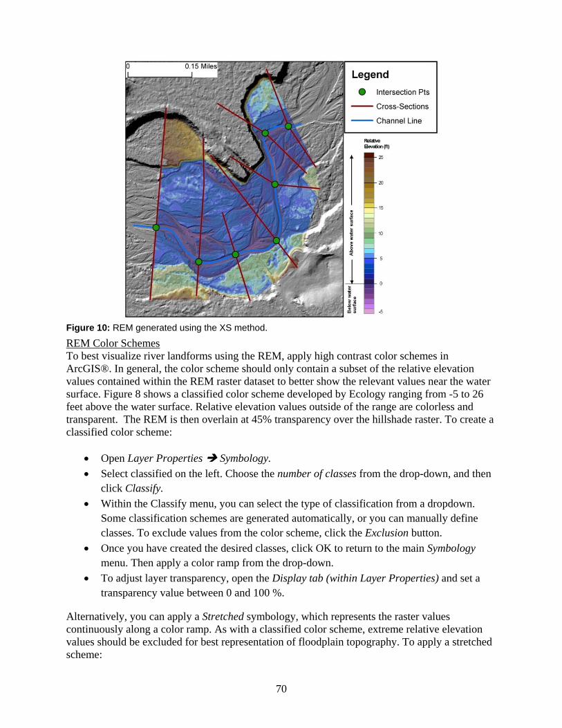
70

Figure 10: REM generated using the XS method.

REM Color Schemes To best visualize river landforms using the REM, apply high contrast color schemes in ArcGIS®. In general, the color scheme should only contain a subset of the relative elevation values contained within the REM raster dataset to better show the relevant values near the water surface. Figure 8 shows a classified color scheme developed by Ecology ranging from -5 to 26 feet above the water surface. Relative elevation values outside of the range are colorless and transparent. The REM is then overlain at 45% transparency over the hillshade raster. To create a classified color scheme:

• Open Layer Properties Symbology. • Select classified on the left. Choose the number of classes from the drop-down, and then

click Classify. • Within the Classify menu, you can select the type of classification from a dropdown.

Some classification schemes are generated automatically, or you can manually define classes. To exclude values from the color scheme, click the Exclusion button.

• Once you have created the desired classes, click OK to return to the main Symbology menu. Then apply a color ramp from the drop-down.

• To adjust layer transparency, open the Display tab (within Layer Properties) and set a transparency value between 0 and 100 %.

Alternatively, you can apply a Stretched symbology, which represents the raster values continuously along a color ramp. As with a classified color scheme, extreme relative elevation values should be excluded for best representation of floodplain topography. To apply a stretched scheme:

71

• In Layer Properties Symbology, select Stretched from the left bar. • Choose Standard Deviations stretching method from a drop-down, and choose 2 to 2.5

standard deviations. • In the statistics box below, change the drop-down from “From Each Raster Dataset” to

“From Custom Settings”. • Adjust the Minimum and Maximum values below to exclude values from the symbology. • Adjust transparency as described above.

The user can adjust color schemes that allow them the best visualization of floodplain and valley bottom topography.