A METHOD OF CALCULA TING THE LIFT ON SUBMERGED …
130
NORWEGIAN SHIP MODEL EXPERIMENT TANK THE TECHNICAL UNIVERSITY u,- NORWAY A METHOD OF CALCULA TING THE LIFT ON SUBMERGED HYDROFOiLS by Harald Aa. Waiaerhau.g NORWEGIAN SHIP MODEL EXPERIMENT TANK PUBLICA TI()N N 71 NOVEMBER 1963
Transcript of A METHOD OF CALCULA TING THE LIFT ON SUBMERGED …
NORWEGIAN SHIP MODEL EXPERIMENT TANK
THE TECHNICAL UNIVERSITY u,- NORWAY
A METHOD OF CALCULA TING THE LIFT
ON SUBMERGED HYDROFOiLS
by
Harald Aa. Waiaerhau.g
NORWEGIAN SHIP MODEL EXPERIMENT TANK PUBLICA TI()N N 71NOVEMBER 1963

LIST OF CONTENTS
THE 3 DIMENSIONAL HYDROFOIL
ABSTRACT
Page
i
2NOTATI ON te OS0eøO0S 0@0000 Q t 0QQ Ott Cotto
THE 2 DIMENSIONAL HYDROFOIL
FUNDANENTALEQUATIONS
THE POINT V'ORTEX . . . . . . . . . . . . . . . . . . 6
¶t'IiE DIPOLE , O O O Q t O O C O t O O QOOtOt 9
THE HYDROFOIL ,,,,,,,,,,,,, ......... 10
CIRCULATION OF THE HYDROFOIL . . . ... . e.,. 18
SUBSTITUTION BYA VORTEX 20
SUBSTITUTION BY A VORTEX AND A DIPOLE ,. 22
THE HYDROFOIL AT HIGH SPEEDS . 23THE CIRCULATION REDUCTION FACTOR ...., 28COMPARISON BETWEEN THE SYSTEMS
OF SUBSTITUTION o o o t . . o o t e o t e e s o , o o o o o 37'
CHORDWISE DISTRIBUTION 0F CIRCULATION .. 1i8
ANALYTICAL MODEL OF THE FOIL ... . . . 59
MOMENT OF DIPOLE DISTRIBUTION 000 63
THE DOWNWASH VELOCITY 66
DESIGN OF A HYDROFOIL 73
ANALYSIS OF A HYDROFOIL ...O 8)-i-
EXPERIMENTAL PART
THE DYNAMOMETRE . . .. .,. ....,,, .. 90
EXPERIMENTALSETUP 95T:: - :::::NsIONAL IZDROFOIL 95
THE) DIMENSIONAL HYDROFOIL lii
DISCUSSION 0t. 00 0 tO O O 00000 116
12)-l.
REFERENCES . . . . . . . . . . . . . . , , . , . 126

ABSTRACT
Applying Kotchin's [1]*com1ex velocity potential for
a vortex in the vicinity of a free surface and the corresponding
potential for a dipole developed in an analogous way, the complex
velocity potential for a 2 dimensional hydrofoil has been found
by substitution of a vortex at the approximate centroid of
circulation, alternatively by substitution of a vortex and a dipole
at the centre of the hydrofoil. The two ways of approximating the
hydrofoil have been discussed. The strength of the vortex and the
moment of the dipole have been determined by satisfying the Kutta
condition at 3/k e. Expressions for the circulation reduction
due to the free surface at finite and infinite speed have been
found and streamlines have been drawn by substituting the hydrofoil
with a) a vortex, b) a vortex and a dipole, both cases with and
without gravity terms. Further the hydrofoil has been approximated
by a vortex sheet and the circulation distribution and lift on the
vortex sheet have been calculated. Some values have been computed
on a digital computer.
An analytical model has been proposed for the
3 dimensional hydrofoil applying the results obtained for the
2 dimensional foil. Further an example of lift calculation and
analysis is given for a 3 dimensional hydrofoil.
A dynamometre suitable for hydrofoil testing has been
designed, and a series of experiments have been conducted to cheek
the validity of the theoretical results.
* See list of references.
i
NOTATI ON
a radius of Joukowski. circle0
b span of 3 dimensional hydrofoil0
e chord of hydrofoil.
g acceleration due to gravity.
h distance from undisturbed water surface to centre of hydrofoil.
k circulation reduction factor for 2 dimensional flow,
koo circulation reduction factor at infinite speed.
i factor in equation of Joukowski transform0
q resultant of free stream. and induced velocities.
r radius0
s distance from transformed circle to centre of Joukowski profile.
length (span) of 3 dimens ona1 foil measured along foil
centreline.
t thickness of hydrofoil.
time.
V total induced velocity vector0
u x-component of induced velocity.
y y- I? It ft
w z- ¡I II Vt
complex velocity potential in z-plane0
WD " of dipole0
WV't It Vt vortex.
A a/i.
Fh depth Froude number, u/VaK0 g/U2.
U velocity of undisturbed flow along x-axis,
W complex velocity potential in '-plane,
incidence relative to chord line.
.4It It II line of zero lift, corrected for
3 dimensional effects, i0e. =4gi4g incidence relative to line of zero lift.
dihedral angle0
' (x) circulation along foil chord.
6 sweep back angle.*J displacement thickness of boundary layer.
E downwash angle due to 3 dimensional effects0b9 angle defining coordinate y through y = - cos
2
3
kinematic visc4tty.
9 mass density.
T1 angle between foil chord and tangent to foil mean line at
point Zjeangle defining coordinate x through x = -(l - cos
r circulation.
in unbounded fluid.
at infinite speed.
velocity potential.
- stream function.
THE 2 DIMENSIONAL HYDROFOIL
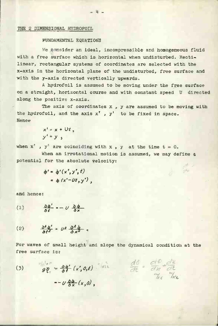
FUNDAMENTAL E QUATI OMS
We cDnsiier an ideal, incompressible and homogeneous fluid
with a free surface which is horizontal when undisturbed. Recti-
linear, rectangular systems of coordinates are selected with the
x-axis in the horizontal plane of the undisturbed, free surface and
with the y.-axis directed vertically upwards.
A hydrofoil is assumed to be moving under the free surface
on a straight, horizontal course and with constant speed U directed
along the positive x-axis
The axis of coordinates x , y are assumed to be moving with
the hydrofoil, and the axis x', y' to be fixed in space.
Hence
XI = X + Ut ,
y'=ywhen x' y' are coinciding with x , y at the time t = O.
When an irrotational motion is assumed, we may define a
potential for the absolute velocity:
4,'- '(x',y',t)4, (x'l./t,y') ,
and hence:
òx
ò24' - ¿j2 O2e?t2 òx
For waves of small height and slope the dynamical condition at the
free surface is:
(3) ò4' /=ai?
ec
.,_,1ò?p (x,O),"òx
dy}/ hi//,(C fè(c.
(4) ò'at ày
- ò4ày
when we define
¿,y_
From (2), (3) and (4) we obtain:
Ò77 ¿jZ ò24'9 àx
=-,or: òy
(5)
with
5
and the kinematical condition
_L_oz4 -ok òx2 òy
K-Bo
'.7jj'a
I ,4 c7d«1jjhe/ r1$c
wheny= O
The boundary condition on the hydrofoil surface may be written:
- ¿I cos (nx).
The velocity components must remain finite when x2#y2co,and at infiniti in front of the hydrofoil there must be no waves,
i.e.:
1/fl,)2
()2}
-*--1' 00We now introduce the complex variable
z = X ¡y
and the complex velocity potential
= 'I j

where is the stream function, and
¿1=- ay
¿1=y ax -
Since
di,' ò+.òIidz - / ÔX
=4;ì&_òx
we obtain
d2w ò24 - ¡dz2 òxX òyòx '
and hence the condition (5) may be written
mn{} im( }o when y = o ,
or
(8) 'n fiì;' =o when y = O.
THE POINT VORTEX
We consider a vortex of strength r/2crr at the point
under a free surface. For this case the complex velocity function
is holomorphic in the entire region yO except at the point
z = , and may be regarded as built up by the complex velocity
of a vortex in an unbounded fluid together with a certain perturbation
velocity due to the free surface, thus:
a'k#'y,C_ / +dz 211 z-

where g'(z) is holornorphic for yO. Referring to (8) we
introduce the function:
E(z) = ¡ dw,dzZ dz
which for yLO may be written:
f f- 2Ti (z-0)2 # ,9(Z)
where is holomorphic for yL O. From (8) we find that
f(z) has real values on the x-axis, hence by Schwartz's reflection
principle it may be continued analytically into the region y> O,
with:
In the region y.O we have:
(9)
1(z) f- (z."z0)2 j; Z
and in the whole plane:
1(z)=¡ ¿2, g dwdz2 dz
r / - 2.r_. i
¡A."_r211 (z0-0)2 2-7e 2iT (z-z0)2 ° 2iT z-z0
with the condition:
¿in, ft'z)O.Z-oo
The homogeneous equation
dwv/ dz2 0dz
has the solution
WV C/
c)t 't"
,
and making use of Lagrange?s method (variations of the constants)
for the solution of the inhomogeneous equation, we write:
(io)
We take:
dC, dC -/Jc'z(II) dz dx e =0,
hence by derivation of (10):
dw d, dC k,z_;j(cC_i4zdz a'z
= - '' C e4'02
and:
-- e' dC e1'('Z -K02 (2e- / ° dz
Substituting in (9) we have:
-M;' z r i+ (zz)]
r, t i(i4) 1e0c,/2 e L(z0)2 02'_i_ 1.z- z-z0J
from which we obtain by partial integration:
z
(15) C2eZ_ L._t_" 7' / \i.i_Ce_'C'oZ Çei('otK0 2Çf2-, z-go) IT j t-0 ¿t
+00
when
òm C,"tim 2Z--?co 2___._
From (ii) and (1k) we obtain:
d_ LI_ tJ
d K0 2 [(Z_Z0)2(2_'Z0)2] ZZ0
hence:
r / f.
rK0 2Ti' z-i0 -0) 2iT ZZ0
and from (io), (15) and (17):
zj. , r e0Z ( ;JY dt.''2TÍ og 2-2e 'rro
From (12) and (15):
dw. r ( 1_ / 2e'otS t-z019) d -, 2i \z-z z-z0
THE DIPOLE
Defining the complex velocity potential of a dipole ofmoment M in an unbounded fluid
D 2ì(z-z0)
we may write in analogy with (9):
We have:
C e'0Z
(20)i, aw, ' 1e e/ dz' '° dz L(zQ3 (z-z)

and taking:
we find:
(21)
and hence:
(2) VD _ ZrIO ti e'9 .,L/ 1t'.// e9ek'.z
2e
z-0 2í z-z0 t-z000
z
(2k) If e fi c-9 ¡ N e , %2,? e'g - ¡/(0 Ç 1k: dt.- 2'ÎT (zi)2 W(zz,)z 'T z-z0 ii j tz0
THE HYDROFOIL
It may be shown (see f.ex.. ) that at sufficiently
large distance from a Joukowski hydrofoil, the flow is that due
to a vortex and a dipole both at the centre of the hydrofoil, ialternatively a single vortex, the substitutional vortex, placed
at the centrold of circulation.
We shall consider these two systems of substitution
more closely. Referring to Fig. 1, the circle V'-ika is
transfonned into a Joukowski profile by:
dC dC+ e"=O.dz dz
N I e(22) Ç#eZ
/ 2rh Lz
z
___ dt-zo
(25)
- lo -
1..d_.. 1e' -io -i1
ioe -/e2'Th.L(z-0) i_z)2j 2'iT1z-0 . z-zò J
e'0 1f e' ; ''")2 (z -Z0)2] T z - i0 ejr

or:
z1*V_422
With this reversal the usual expression for the complex velocity
potential in the -plane of a circle with circulation:
L/ = (le '°' ¡ 2T1 -s)
or, since s for thin and comparatively straight profiles is
very small:
¿/e4Ca2(27) 2q-r
¿O9.(
(26)
may be written:
li -
FIG. i

-. r
- 12 -
, -/ 2Ue a, (/ec (zv/z2 4L/Z,)#2'#Vz'2_4c122
tr
¿ 2]2'Tt
For a hydrofoil moving under a free surface, it is more
convenient to use the axes x, y of Fige 1. We then have:
Z'- Ze'
and:
e' (ze°'# /_2')# 2¼a2 . iogze1#i2(2 ze'vÇ' Z2'fT
211a2 r r.' V- ae12 #1 j z '
/ 2# Ic'
2 2 /1
¿'e
where the constant K may be omitteth Equation (29) may also be
written:
2V_Ì2i2 /1O9(30) w=k# z
"e) yt2_2/2oc)z
z /2
.
f-
)
I liC2ee
z
z
Writing:
(32)
¿o-2
21T
we obtain:
(31) 20Z {i_
and when
I. '?ií./(a2-1'e ¡2.0
r' , (t /_(2e14')ì
is small, we may write
,2Ç1() (at_/2ei2oC)
r
13
t',
¡ t_il.- .r
/ (2/eYiiz V'vP'; ¡ log ',
{e
2 ,2G'4' (2/e')Z2
ext-irz1f#/ (2/«. )
-
f_(21e)2 ;2u(a/zei2L 2 r2
For a flat plate in an unbounded fluid, we have
r= '-i-r ¿IL sin oC e'
and consequently
20.leb0C ,
When z is large, we obtain the usual, approximate expression for
the centroid of circulation as given in f0ex. [3]
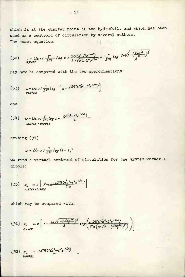
(33) L./1Jz#i1ogVOR7TX
Writing (3k)
k'=
we find a virtuel centroid of circulation for the system vortex +
dipole:
(35) ; - z { I-exp-;241
¿('02_12e ¡2
JrzVORTEX *D(POIJ
which may be compared with:
- 1k -
which is at the quarter point of the hydrofoil, and which has been
used as a centroid of circulation by several authors.
The exact equation:
/ 121e" )2¿1(a_I2eo) 1'l/t- z(30) w=lJz#i 2fl' 2 4/2121C 2
(XACT
may now be compared with the two approximations:
/_2e/2C)z
VORTEX # DlPOLi
r ,2TrV(o2 12.c)]
12 r
z20 - 2 [ I f'.k4' (21iøG)zexp(i4(rr1/(a2_Zze ¡2.G)
2 rzEXACT
z¡2J(a2_4')
rVORTEX
- 15 -
o
FIG. 2

- 16 -
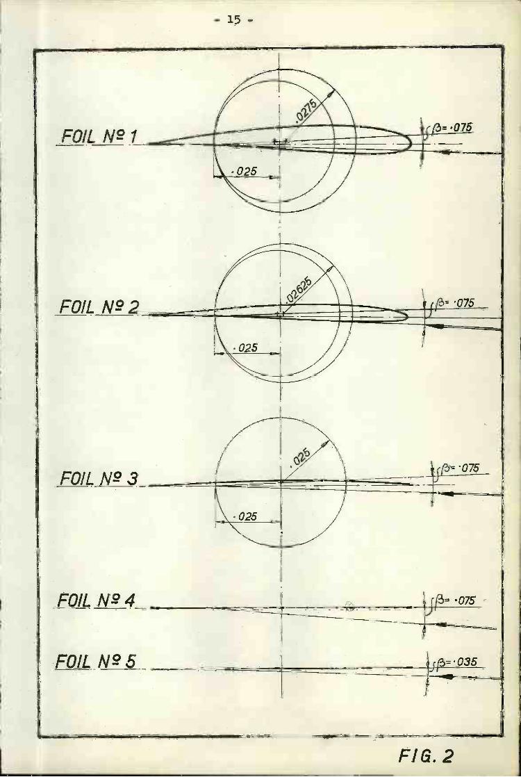
As a practical example we choose
i//C
¡21e aMd /e
and consider the foils defined by:
i = 0.025
a = 0.0275
oc 20
=
i = 0025
a = 0.0262500c= 2
»3 =
i = 0.025
a VT
20
/3 =
k) 1 = 0,025
a t?
I O= Lf3T?
5) 1 = 0.025
a
20
/3
The 5 foils are shown in Fig. 2.
Further we define the circulation
P=zj 4'uia tJsìn,4
where k = i in an unbounded fluid, and where k#1 in the
neighbourhood of a free surface. As an example we choose k = 057
and k = 029
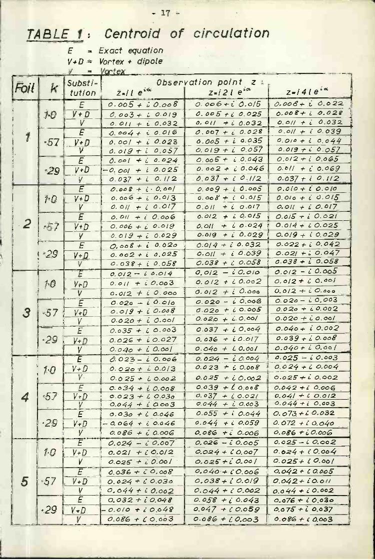
TABLE 1: Centroid of circulationE = Exact equationVD = Vorte> # dipole
a
I ,' Substi-1tutfon
Observationzil e'
point zz=i21 e zai4ie'
lQE o.ôo5O.008 o.òc6*zO.o/5 Ò0C+ O022
V*D O. oo3 -t- . ooi o. cog , 0.025 ö.cc8'+ ¿ ô.oV ô. O/i -t- i. 0.032 . °1/ # ¿ 0.032 C.c// -t- ¿ 0.032
57 E o. o .'. ¿ o.oi 0.007 1- ¿ o.02g 0.01/ -e'- 0.039_VD O.00/ - ¿ 0.023 ô0o5 * ¿ 0.035 0.0/0 - ¿ 0044
V O. ô/9 -i'- ¿ 0.c.57 O, 0/9 -t- ¿ 0.057 0.019 i- ¿ Ò.57
29E Ô. cI -+ ¿ O. 024 O. ocG i ¿ 0.O3 0.0/2 - ¿ O,o5
VD -c ô, + ¿ 0.025 0. ö 4 ¿0.04e O.b// - ¿ OO9V 0.037 + ¿ 0.1/2 .0.037 - 0.1/2 0.037y-/ 0.1/2
7.0E -- ¿. ûoo/ o.009 -t- ¿ OooS c.Ó1ô-t. ¿ c.oic
0.ôo-t- ¿ 0.0/3 O.00-t- ¿ 0.O/5 0.0/o + ¿ cJ.O/5V 0.01/ ,'- ¿ ô.017 o.ô/f ¿ oöí7 o.oi/ . ¿ .0/72E.57
ò.o(i -t- ¿ Q.00 0.0/2 .,'- ¿ 0.0/5 o.ö,5 - ¿ 0.021V+b o. ôo, ¿ 0.0/9 0.0/f -i'- ¿ 0024 0.0/4 -t- ¿ 0.025
y ô.öi.9 -t- ¿ 0.029 o-dg -t- ¿ 0.029 0.0/9 -t- ¿ 0.029
'29E -t- ¿ O02o C0/4 -t- ¿ 0.032 0.022 .'. ¿ 0.042
V*D O. oo2 # ¿ &025 0.01/ -t. ¿ Ô.O39 0.021 0.047V C. 3g -t- ¿ ôo5g' 0038 -t- o.o58 ô.03e ¿ 0058
3
1.0E 0.0/2 - ¿ 0.014 00/2 - ¿ 0..oío 0.0/2 - ¿ C.005
Vt-D 0.0/i -t- ¿O.003 0.0/2 -t- ¿C.ôo2 0.0/2+ C 0.00IV 0.0/2 -f ¿ O,öoo 0.0/2 + ¿ Oôøö 0.0/2 ¿ Ö.ôa.o
57I E 0.02o - L O.O/ 0.020 - ¿ 0,o 0.o2o ¿ 0.003
EVD o.o/g + ¿ O.ôo9 d.02o # ¿ O.005 0.02o -t- ¿ 0.0020.020 -t- C coot
V 0.020 + ¿ OooI 0.o2ö + ¿.C.ööJ
29E 0.ö35 - 0003 0.037 -t- ¿0.004' o.04o ¿ 0.002
VD 0.ô2G -I- ¿ 0.027 0. o3, -t ¿0.017 0.039 -- ¿ o.006'V 0.o4o + ¿ Ooo/ O.04o -t. ¿ 0.00/ ô.c40 1- ¿ Oôö /
4
7'Q
- E ó023- ¿ O.00 0.024 - ¿ 0.004 0.025 - ¿ 0.003V+D 0. 02o -t- ¿ 0.0/3 0.023 * ¿ 0,009 0024 .t- ¿ 0004
V. 0.025 ¿ O.ôo2 0.025 * ¿ O,002 Ö.025-f--i 0.002
'57-
E 0.034 -# ¿ OÖoê 0.039 * ¿ Oco6 0.042+1 0.00GVtO 0.023 + ¿ 0.030 0.037 ¿ 0.02/ 0.o4/ +
V 0.044 - ¿ Cô3 ao44 -t- ¿ c.003 0.o44 -e.- ¿ 0.003
'2.9E o.03c -i'- ¿ oò4 0.055 * i O.o44 0.o73+C 0032
Vi-D -0.o,4 - ¿ o.c c.c44 - ¿ 0.059 0.072 -i-iÖ.o4oV e'.o96 + ¿ Ô.ÖO C.og +C O.oÔG C.Og -t-COOoG
5
1.0E O.c24 - ¿OOo7 0.0.2 -00.005 0.o25-'..0.002
VD 0.. 02/ + ¿ 0.0/2 0.024 - e O.007 0.024 + ¿0.004V 0.025 + ¿ OôôJ O,.Ö25* 00o/ 0025.t- ¿
'57E O. o3 -t- C 0,. oô9 0. o4c - - o. o42 c o. co5
. Vt-O 0.02-4 -t- ¿ O.03i 0.038' -t- ¿ O.oiQ 0.042 ¿0-0/1V O.e44 O.co2 0.044 ¿ 0.062 oo'i4 + ¿0.002E 0.032 -i- ¿0.049 0.059 ,'- 0,043 Ö..ö7 * ¿ C.03o
29 V+D - o.o/o -t ¿ oo4g 0.047 -i- C 0059 0.075+ ¿ 0.037V c.ôS -t- C o.o.3 0.o9 + ¿ O.003 O,o -t-¿ 0.003
18 -
With the given values, Table 1, of z0 has been computed.
Some information may be obtained from this table:
In an unbounded fluid (k = i) , substitution by a vortex and
a dipole at the foil centre as well as substitution by a vortex
at the approximate centroid of circulation, both give a good
approximat1on to the complex potential at a distance from the
foil at least equal to the foil chord.
As we approach the hydrofoil,substitution by a vortex seems to
give the best approximation to the potential for infinitely
thin hydrofoils, whereas substitution by a vortex and a dipole
gives the best approximation for hydrofoils of some thickness.
The quarter point may be regarded as ceritroid of circulation
only for infinitely thin and straight foils.
In the nei:hbourhood of a free surface k1 , substitution
by a vortex and a dipole at the foil centre seems to give the
best approximation to the complex potential at all distances
from foils of finite thickness. For infinitely thin, straight
or curved foils, there seems to be little difference between
the two systems. Substitution by a vortex at the quarter point
is in no case permissible.
The effective centroid of circulation of a hydrofoil In
the vicinity of a free surface is not the same as that given by
z0 in (31), (32) or (35), since the image system will influence
the velocity distribution. This will be shown later by substituting
the foil with a vortex sheet
CIRCULATION OF THE HYDROFOIL
In an unbounded fluid the circulation around a Joukowskiprofìle may be evaluated in the -plane of the Joukowski circle
by making a stagnation point the point which transforms into the
trailing edge of the airfoil, I.e the point -le" Strandhagen
and Seikel ¡2J applied a related method for evaluating the
circulation around a flat plate hydrofoil under a free surface They
substituted the flat plate by a vortex at the i/k point, le" ,
and satisfied the Kutta condition at -le"'
- 19
In this paper we consider the flow around a Joukowski
hydrofoil of finite thickness and in the vicinity of a free surface
as approximately equivalent to the flow around a dipole and a
vortex of suitable strength at the centre of the foil together with
the images due to the presence of the free surface. In analogy
with the case of unbounded flow, we now regard as "undisturbed"
flow the free water stream together with the disturbances due to
the image system. The circulation is found by making the point
on the Joukowski circle a stagnation point, we then consider
the perturbation velocities at -le1" in the zplane insteadof in the plane. This may be done since the perturbation
velocities at leC re approximately the same in the z-plane and
the ' -plane. By derivation of (25) we find the velocities in
the z-p1ane
dl'dz dl' dz
dw
Hence the flow at some distance from the dipole and the vortex,
i.e. for large '// , will be approximately the same in the
z-plane and in the r-plane. We shall discuss this at the end of
the paper.
The considerations above will of course also be valid
when the hydrofoil is substituted by a vortex.
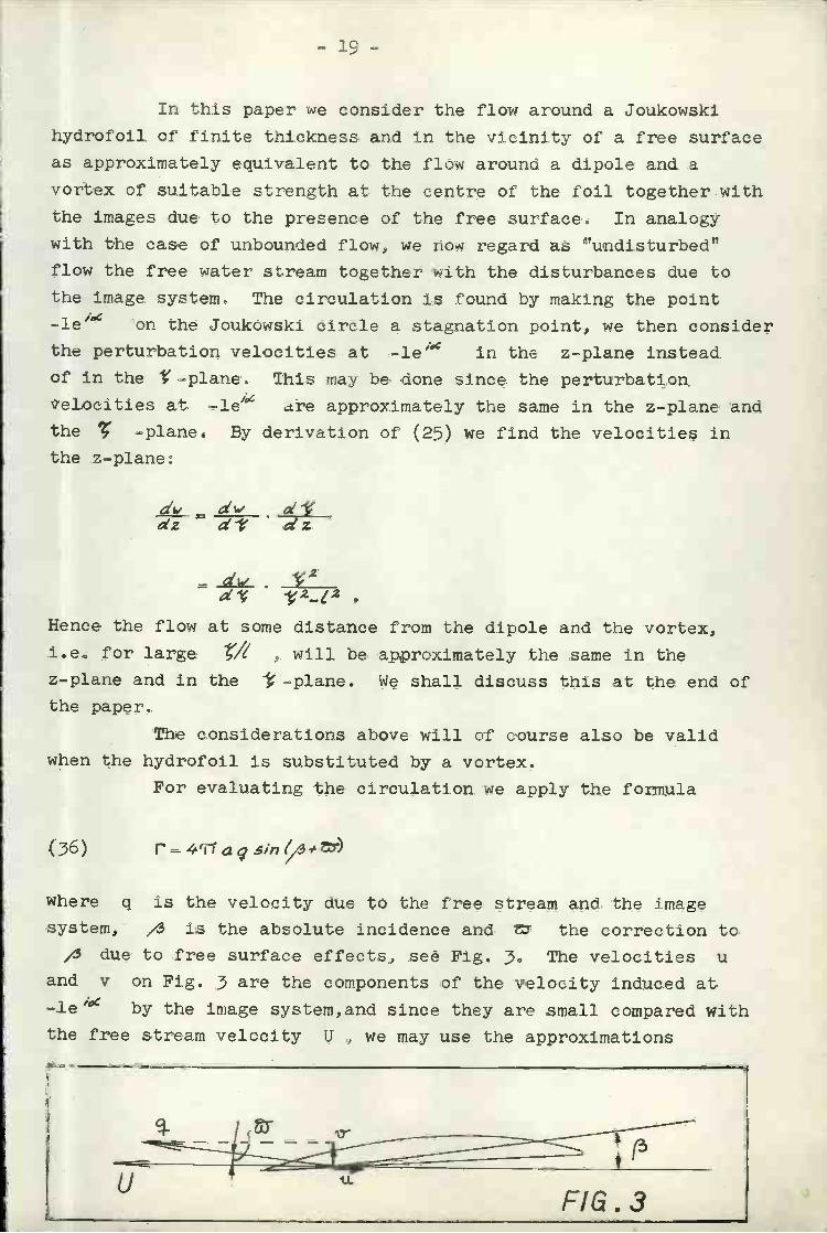
For evaluating the circulation we apply the formula
(36) P=4ia, Sin
where q is the velocity due to the free stream and the image
system, ,4 is the absolute incidence and the correction to,3 due to free surface effects, see Fig. 3 The velocities u
and y on Fig. 3 are the components of the velocity induced at-le' by the image system,and since they are small compared with
the free stream velocity U , we may use the approximations
t
or:
41Ta(U-u)(/3* )=krra«From the last equation we obtain:
4 (-4ç; iì )
SUBSTITUTION BY A VORTEX
Approximating the complex velocity potential of a
hydrofoil in an unbounded fluid by:
r=br', ,
- 20 -
'- ¿Iu
I,,
¿1-
For thin hydrofoils the angle ,4# is small and
1cin (/3# /34.With these approximations (:36) may be written:
y
Denoting the circulation of the hydrofoil in an unbounded fluid
by Ç , we define
(33) w(Jz#if ¿og [ /2ci(1(#a2_1Le20c)1

and putting
- ¡2'rru(2 I2OCa-Le ) 1/,z0 = r
- -i2'TWe'a2- l2e12' ) ,20 rwe obtain with reference to (19) the complex velocity due to the
image system:
(40) 2'
dz 2T( z ,.,,
21
eìA'e dt.¡h
(42) " = i - ' - e' b 4a ¿j' (-le 'A) e dt
For thin profiles, we may use the approximation
and
20-;2r(1J (I - éc)
= ¿Si»ol ek
or:
(ki) z0., e'°'# iii
With this 1.st approximation we obtain for the complex velocity
at -1e'-ih due to the image system:
-le hh1c/h
¿11 J2T(V(a2- ¿2e-/2.r*14
S
and
VJrr7
we may evaluate the circulation reduction factor k of (38) using
(21.2).
SUBSTITUTION BY A VORTEX AND A DIPOLE
If we approximate the complex velocity potential of a
hydrofoil in an unbounded fluid by (see (34) ):
(43) w/z#i-2-1ogz ¿/(a2_12e121C)z
and put
('ti
we obtain with reference to (19) and (2k) the complex velocity
due to the image system:
z
dw, =.;_[_ /dz 2i z-1h t-;A dt
£
_L._ e'8 ./k' N e ,'2.JL. i9e_'0Z Ç ,'4Y2í (z-1h)2 O IT z-1h o \ tii di',
or, at the point -1e'-ih- ¿'e
' ,Adw - ¡ 421/a srnSdz - le°- ¡ZA k, k 41/a 8ífl/ iÁ'
(-le ''-1it) Ç g dtf-lizcO-le '/A
ík,tdt¿Ja2 ¡K 21/a2 K22¿Ja zj 14 (-le 'i. ¡h)
('.1e'"-l21') -le i'd_124
k .-eHt -o)-
- 22 -

-23-
../ '-í1i
ic' 2012e -20C I e IkOt dt.(-te ''-2h)2 -' ° -c '-i2A t -liz00
This is a more convenient expression than
when evaluating the circulation reduction
the hydrofoil by a vortex and a dipole at
foil.
THE HYDROFOIL AT HIGH SPEEDS
From (18) and (23) we find the complex velocity potential
for the system vortex + dipole at the centre of the hydrofoil,
i.e. at = -1h
zz ¡h r - f14, z C(46) wUz-/f.tog
co
N e'9 N i'9 #/1_ejo2 C e°t29T z*/h 2T1 z-1h O9 \ t-i dt.
At high speeds when
the complex potential approaches:
(47)
M e'8 ÌY e'8'2'íT Z.'ih 2T z-,h
j-2w
(42), and we shall therefore,
factor k , substitute
the centre of the hydro-

With the approximations:
-/e''-/2A------- 121z
and denoting
I/
fl f.= -
we obtain from (49)
'A(50) a ¿í"kM -4 P s2oc' - i c
82
1'
i T ços2ac - T - 7.42-Ávoo=
2k -
or:
t,= ¿'z . ¡b 2 ¿la gi,/ ¿09 (z ¡h) ¡k 2 ¿Ja sin/3 log (z -¡h)
lía2 ¿Ja2 tí2eI)G jj/2 ez#ih Z-lA zìA .
An expression for the complex velocity at the point -le°- ¿kdue to the image systems is found from (45)
dw...; A2Ya ¿J&
dz / 1e '° -,2 /z (-/e,.,)2
(-le 'K ¡2A )2
25 -
The circulation reduction factor is from (39)
j=i
.a_, V¿1 ¿1,4
and using (50) we find the following expression valid at high
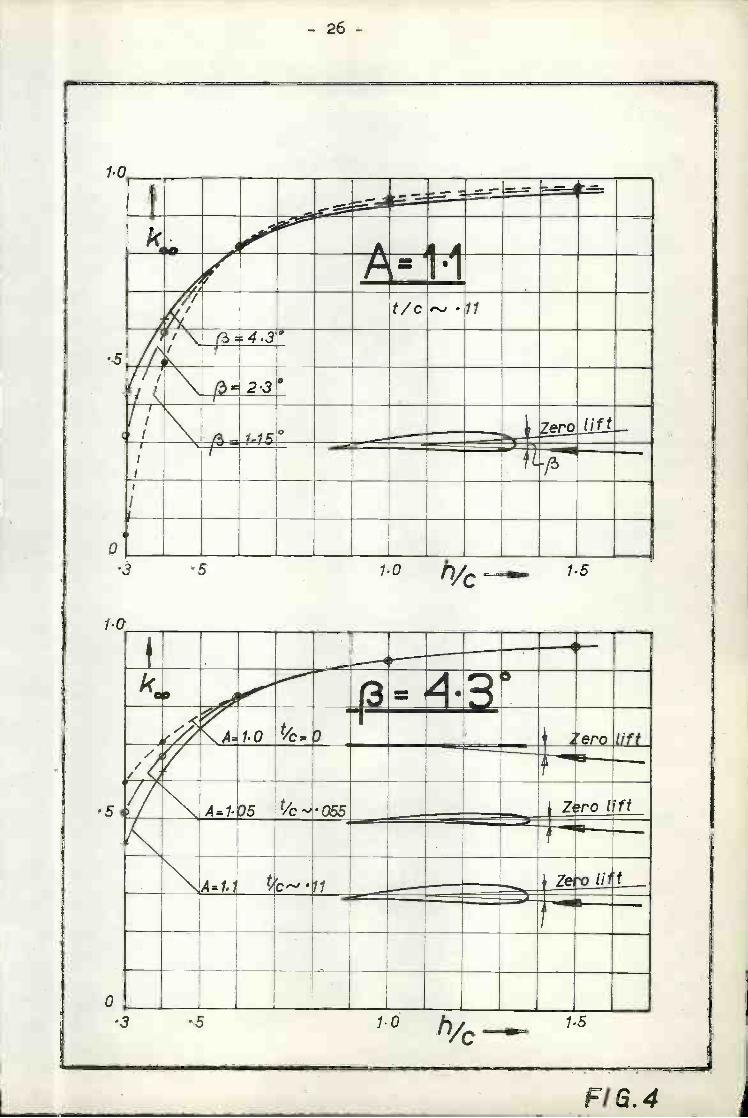
speeds:
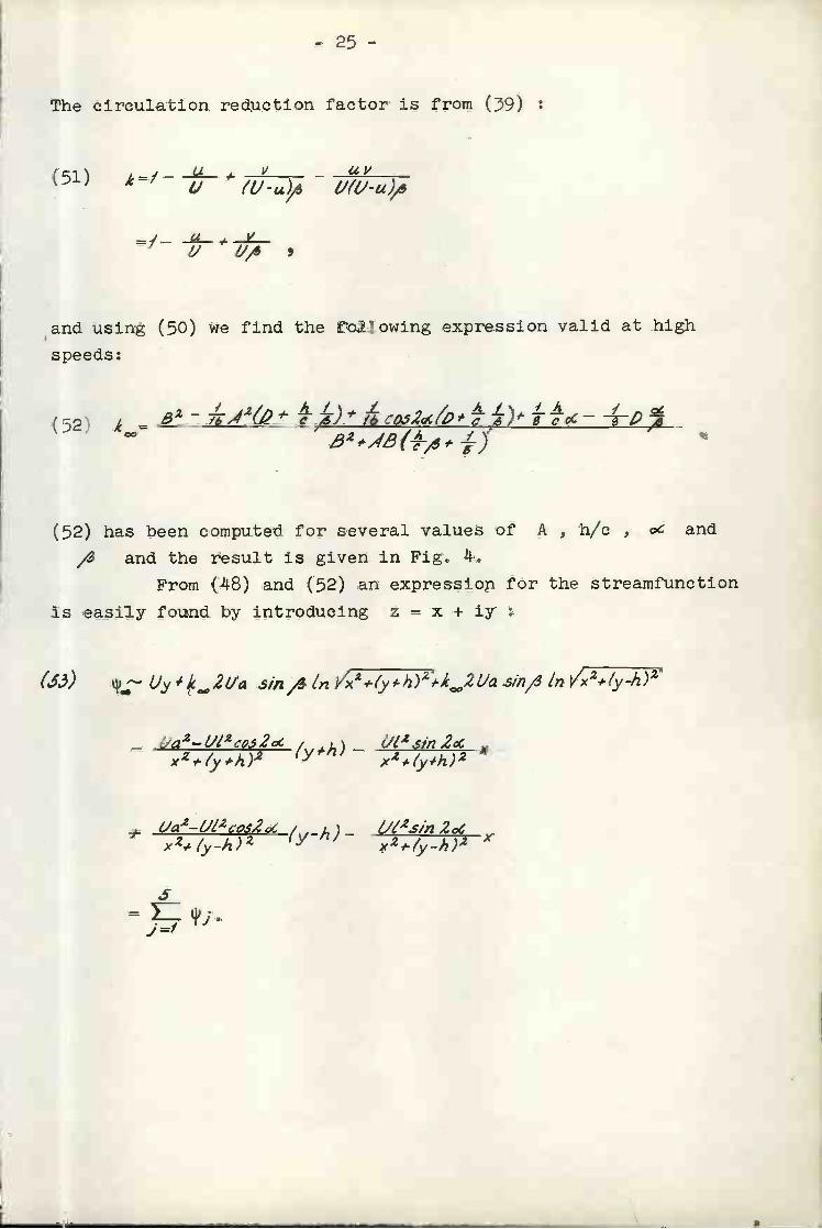
(52' A00-- z( n-),' 4 coi2oc(ßt t,f)' LA i' o
82(Á i)
has been computed for several values of A , h/c , o and
4 and the result Is given in Fig0 .
From (11.8) and (52) an expression for the streamfunction
is easily found by introducing z = x + iy :
(6.3) Vyik2Ua s/n,4 ¿n y/2*(y,.h)2.A 2Va sin,, ¿n Vx2(yh)2'
=/
¿la2- ¿l/2o2 (yi'h)
* ¿la2-E1/2,2 (y h)
5=
XX2 L (y'h)2
¿/'21/fl 22X
- 26 -
FIG.4
1.0
5
o.3
10
-W--.-
_-=_-=-=:--
kUir A=1'l/1'/ t/c''11
-
[3r43/I'\\o 11f
.5 10 h/c 15
ILI_________
A.
1/f t
5 U.A =1.
1-ro 1f ft
/c ii __________________ Zero lift
Û
4
lo h' ___ 1.5¡C
- 27
the 5 parts of which may be written implicite like:
(54) y
(.55) x2# (y#h)2 - (ep4 )2
)C:Z ,' ( 42)2 - (eXpA 21/a s/n/s / '
(U2sin2oC 2
#12 # (ai4_2a2/2os.2ot)2L) ,
(59) * [ /z - - (a2_I2as2oc)}= (a#/-2a2/2c,s2oc,).
When the circulation reduction factor for the foil at high speed
is found from (52), it may be more convenient to substitute the
hydrofoil by a vortex at the appropriate centroid of circulation
expressed by:
(5Q') / (a2-í'e i2) h- A2as/n/3
At high speeds we obtain the complex velocity potential:
,ia*_¿2/2oC)
(60) -Uz*iÁ2(Jai/n/J1og { 42a
.
#-ik,211a 6/fl/ ¿[
and the stream function:
k,2a d/>?

we find
28
=(Iy ,'Aoe2tJa sfn,,4 ¿a y"('x ¿'im2oc 2 / a2-c'2co.c2aÁoe2a 5th) IY 2a
# k 2 ¿la g/n,/ i /( ¿25in 2 c 2 / a212co52Áoe 2 a ( Y 2a GInA
h )2
=.
or
W'¿1 '
( ¿2.9in2o '\2 a2-tcos2oc \2 /Áoe2a /n,,4 /1
Aoe2a (/?,) -Çe
(6k) l25jn2oC \2
( , * a2-Ico2c '2 / 2
Aoe 2a 2 a= (e oe2aUin)
THE CIRCULATION BEDUCTION FACTOR
Substituting the hydrofoil by a vortex and a dipole, we
shall find a general expression for the circulation reduction factor
k , and consider first the integral:z
(65) T=e0hS eY dt
Introducing
¿ =k('h)
)2
J
(66) 7=e_2K0
oo
e' da
D,r #iZ/-4)
or, withC
X
y=-Á
(67) r=_e21co e"
-K0 -;21t,Á
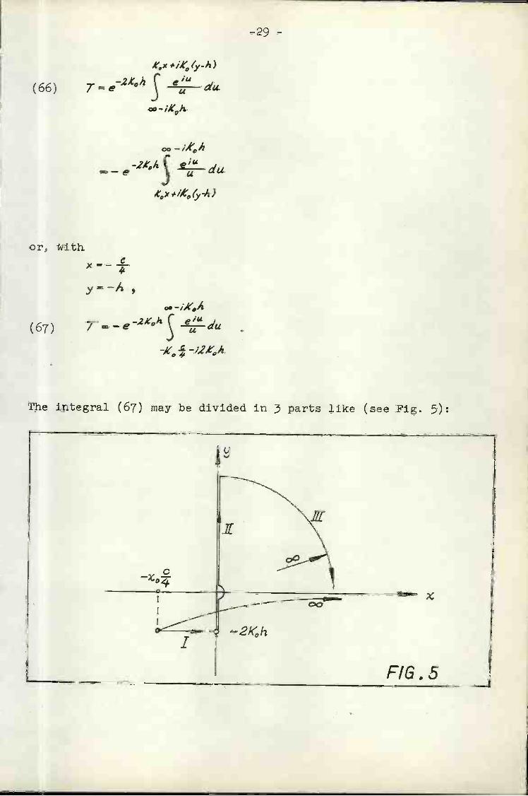
The integral (67) may be divided in 3 parts like (see Fig. 5):
-29 -
/00-24'0h
(68) T = - Ç e duS
Q/U au #S
e ¿L du-i2K0h -/2Kh
e2Koh
The last integral3 III, is equal to zero9 and the remaining 2 may
be developed as follows:
(69 i
If#14
'urther:
-0-2N,A
I, = - du u du
- -/2K04) * Ûc'o -i2kA)
= ';(ì'f " Ci(í24Ç i»
and:
-4 -2K0/z;=-/Ç '1' du
-/20h
-12123 -2K0h
Ç 03 ¿ du . / Ç sÑ u duu
- -i24 h - h
-2k;,fr-e
31
--S;(-K0 -,2X0A)
- /3'! (i ;'4 L
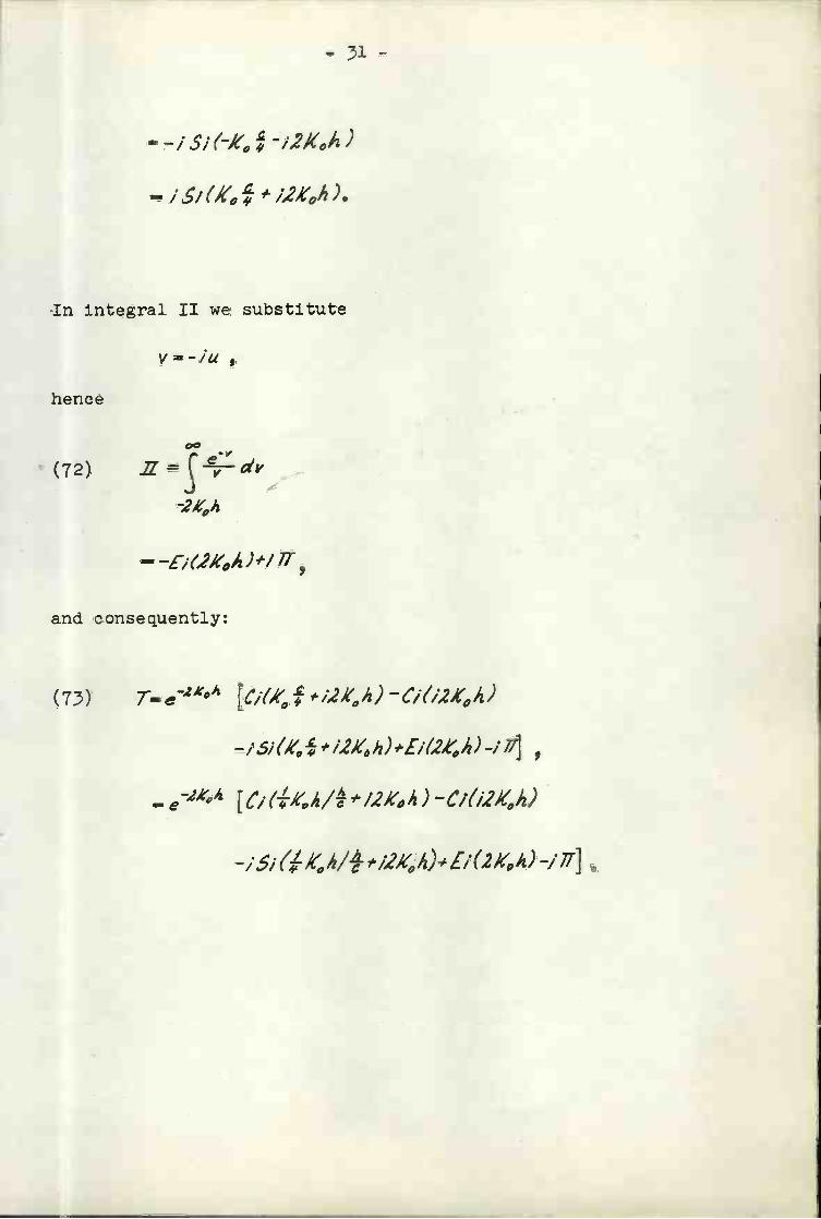
In integral II we substitute
V-/L(
hence
r &'
-2AÇIz
- E«JK0h )#/ iT,
and consequently:
T_ie.21'0'1 {C/(/(,f*/2A'0h»C/(/241z)
[C,(*k/# i2Koh) Ci(/21c',h)

- 32 -
With the approximations
_1e"_/2#4sf -/2,4
and
I/fl S#/4
we find from (k5) the induced velocity at the point ('.- - 1h)
due to the image system:
.- -/4
(7k) 42/Ja Ç eAt¿t-/21 D ) t-1h
00
--i,¿la2 A',21a.L # 2(a2e16"f et
(- -,2h)2/ /2k t -1h dt
Co
¿/Icoo2oc / 2cJtc, K,2//2o2oc(_J2%,)2 (_/21z)2 /
KD22O1eCOs 2oCe''' C
--/2h dtCO
-i-iA# K2/2oe'0 (-J-1h) Ç
ejt-,½
dz'.
With the abbreviations:
(75)
FR
EE
SU
RF
AC
E
Line
of z
ero
lift
r .
FR
EE
5'L
/RF
AC
E
zero
!1.
/3 =
4.3
° co
nst.
h
lo
Line
oft/c
O-O
.O6
-uO
'l1
4.3
3.15
2
---
.4
U9u
IPuu
I!IP
uII_
___
_i _.__
__Ii
34
58
78
9lo
F
15
- 35 -
E ,4s/n X - co.s gin X 2C CO.9 X
T4Z cos A o2c C06 )2'c .5/fl A
6 =sin À *,,4co A
N =,. .in ).. - CO.5 A
,,_ì-i AL
L
and the approximation
¿fl%d,
the circulation reduction factor derived from (51) and (Vi.) may
be written down in the following form:
(76) A 32",4BLAAß2 [C,FeTmI/JmT]
#
#A [LCo62
c,3j
#2A2ß2 [(Çt*r),peTt (,F)Jm TJJ
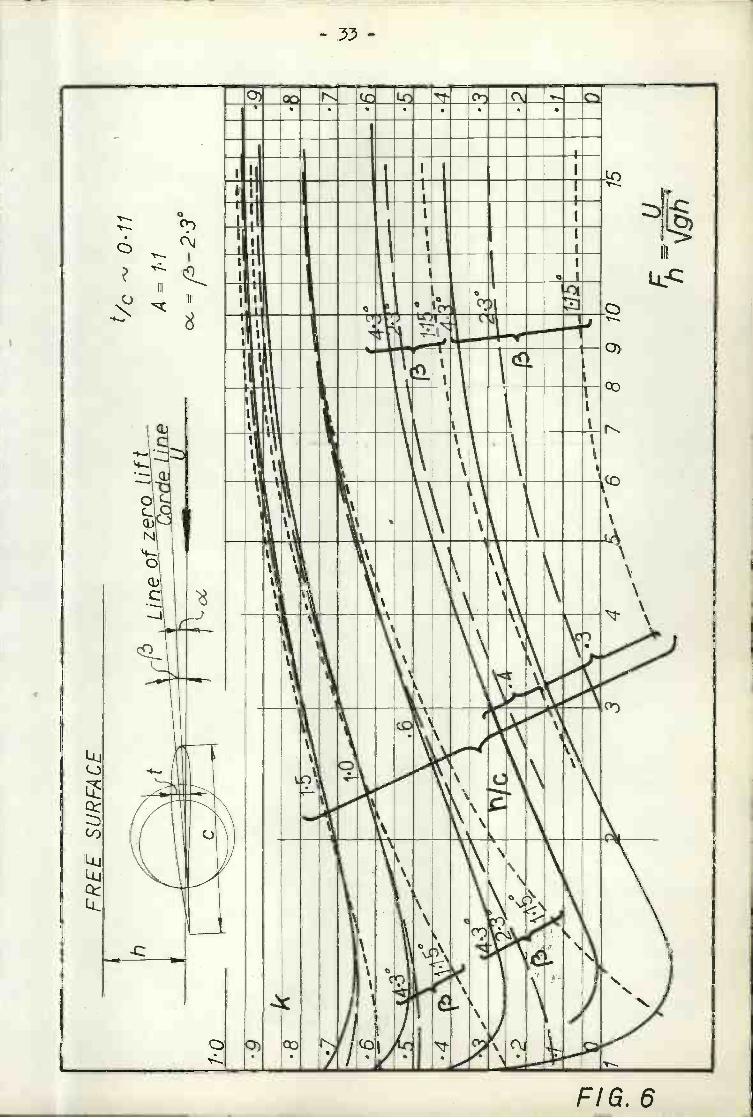
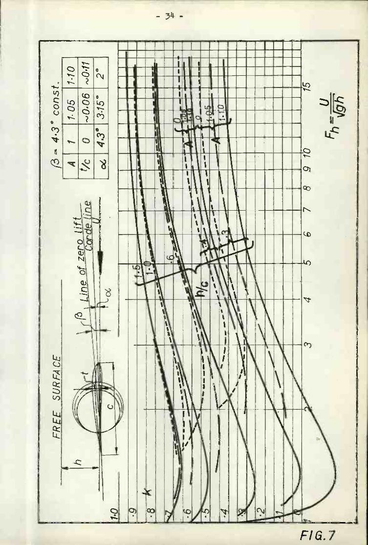
With K0 = 0, (76) reduces to (52). (76) bas been evaluated for
several values of a/i , h/c , U , oC and , , and the result
is shown in Figs. 6 and 7.
The calculations were performed as shown in Table 2,
and for the smaller values of K0h, the following approximations
have been found to be sufficiently accurate:
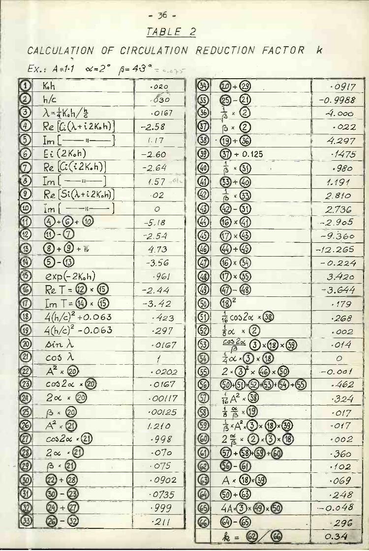
- 36 -
TABLE 2
CALCULATION OF CIRCULATiON REDUCTION FACTOR k
Ex.: A=11 c=2°
® .020
© si/C
© A01/ .0(67
-2.58((7ii
J
(2K0h) -2.60[C(c2I<6h)] -2.64
® rí- 1.57' ]
® R.[S(1\.+26h)) 02
©Irn[ J o
® -5.18
© D- 2.54
© ®++T 473® ©-©© exp(-2K0h)® -2.4i© LmTx® /c)2+o.o63 23
® (h/c2 0063 297® 01G7
© coX y
® A2 x 0202
® co2o xJ 01G7
® 2o<. ' Oo/!7® f? '00/25
® A2 1210
© .99g
j::i 2o -070
© «-'® 075® .0902
® ®-® .0735.999
@ '2/I
I® +® -09/74 -® -0. 9988e -® .o0o
,® r»© .022® 297® ®0.125® ® .98°® ©+ (.191
© ® 2.8/O
© -® 2.73C
® ©x© -2.9c5® 9.3,o® -/2.265© ®x® -0.22'© 3/'2o© ©-© -3.644® .179
® co2o '268(J .002
© co2& .0 r'-
o
®® ©+++© A2,(® ¿324
© k-© 017© xA2x©x@x® C17
® 2®ÇJ® '002® ©+©+c
f02© ô.9® 2483 Ax®x® .- oo48
'29e0.34

-37-
Si (4-K,h/# i2JÇ,1z) '
124',h) 0.5772 '. {(/Á)2#(2Xh)2
2/61z1 iaia,?
6' o 'C
These approximations are readily obtained from the general
expressions for Si(x + iy) and Ci(x + iy).
COMPARISON BETWEEN TEE SYSTEMS OF SUBSTITUTION
We shall make a comparison between the systems:
Vortex
Vortex + dipole
Vortex + gravity terms
Vortex + dipole + gravity terms
The systems a) and b) may further be divided into:
a)1 and b)1 r=k ça)2 and b)2 r=kr
For systems a)1 and b)1 the effect of gravity is disregarded
altogether, whereas for systems a)2 and b)2 the effect of gravity
upon the circulation is taken into account although the gravity
terms in the complex velocity potential are disregardedWe shall compare these 6 systems and choose 2 particular
h/c= oiiU = 6 rn/see
= 2°
/3 =
k = O57k00= 0.63
cases:
i) A = 1.1 This gives:
C = O1 m = 9.6
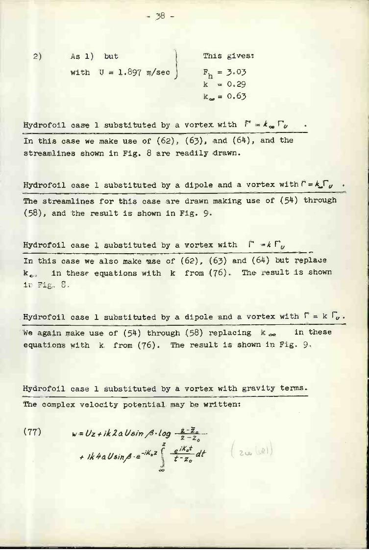
2 ) As 1) but
with U = 1.897 rn/sec
This gives:
Fh =
k = 0,29
k= 0.63
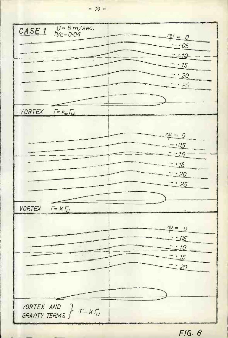
Hydrofoil case i substituted by a vortex with r = k fl,
In this case we make use of (62), (63), and (6k), and the
streamlines shown in Fig. 8 are readily drawn.
Hydrofoil case i substituted by a dipole and a vortex with r=kj'e,
The streamlines for this case are drawn making use of (5k) through
(58), and he result is shown in Fig. 9.
Hydrofoil case i substituted by a vortex with r =k r
In this case we also make use of (62), (63) and (6k) but replaue
k, in these equations with k from (76). The result is shown. -
_Lt
Hydrofoil case 1 substituted by a dipole and a vortex with r = k Ç,
We again make use of (5k) through (58) replacing k,,, in these
equations with k from (76). The result is shown in Fig. 9.
Hydrofoil case i substituted by a vortex with gravity terms.
The complex velocity potential may be written:
(77) w=Uz#ik2rillain,41o9 £ìb2
# ika um .e/X02 e'° dt ( :t20
- 59 -
FIG. ê
CASE1 U=6m/sec.
.O5
15
2O- '25
VORTEX r=kr
_ --- oQ5
-
VORTEX =k1,
VORTEX AND
GRAVITY TERMS I r= k

- ko
FIG. 9
f10
VORTEXDIPOLE r=
VORTEXDIPOLE r- kr
- 05
VORTEXDIPOLE 1GRA VI T Y TERM S J'
r- kLJ
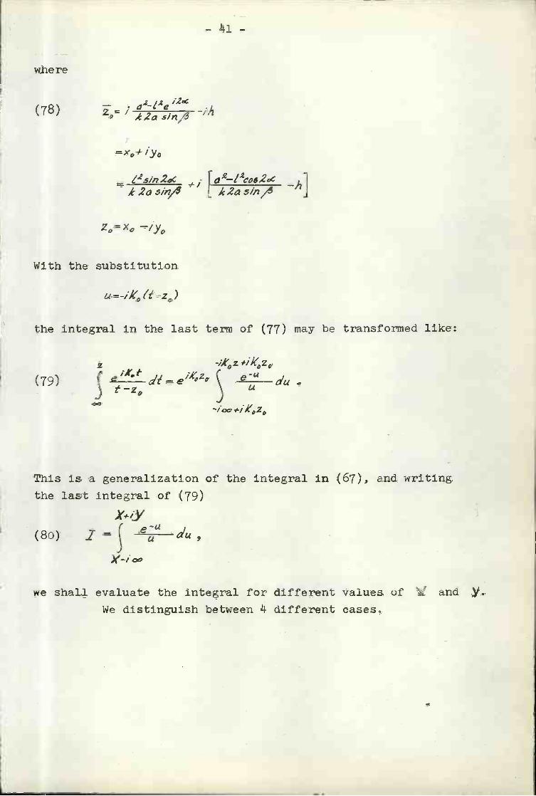
where
a2-t2e 12CC
¡1Zo=/A2a$jn/3
=Xo 'Yo
¿5ii72oC Ia2_/2c62ack2a5/n '
j k2a5m h]
zo=xo -/yo
With the substitution
a = -,h', (t 20)
the integral in the last term of (77) may be transformed like:
z -;Áz 'ik'0z0e 6¡A;z0 e dut-z0
ocOc z0
This is a generalization of the integral in (67), and writing
the last integral of (79)
7 = du
we shall evaluate the integral for different values of 'X and Y.We distinguish between 4 different cases
-
In 1. quadrant we have:
x,y
(81) e" du
x#,y XÇ e da * S
e"
X
=z,' iz7
In integral we substitute
a = -iv
and obtain-y/X
IVdv
ix
-y#,X oc X _yI/xC O5V=
Vdv # # i s/nv V dv
oo#1X ¡X ¡X
'- y ¡X) - C/(1X) i .5, (- Y' ì')
Further
e" du
X-ioo
42
X
=Ti(-X).
Hence, with X + IY in 1. quadrant, we obtain
1, Ci(-Y*i X) -C1iix) ¡S (-Yx) #L7 (-x)
e a'u
= Cì( Y/X) -cjX) -is,(» ¡ Y) *Ei(-X) # i ri'.
The second case is
e du
X,00
=C;(YiX) - C/(/X) -, 5/(Y*iX) #(j(X) -
In 3. quadrant:
-X-iX
(81#) Z =ÇetduJ jUX-
- 11.3 -
-C,(Y/X) - c(ìX) + ¡ 5i(Y íX)#Ei(X),
and in 4 quadrant:
X-i)'
(85)
X-ioo
C/(Y#IX) -C('Y) # ï 61(V*IX) #[ (-y)
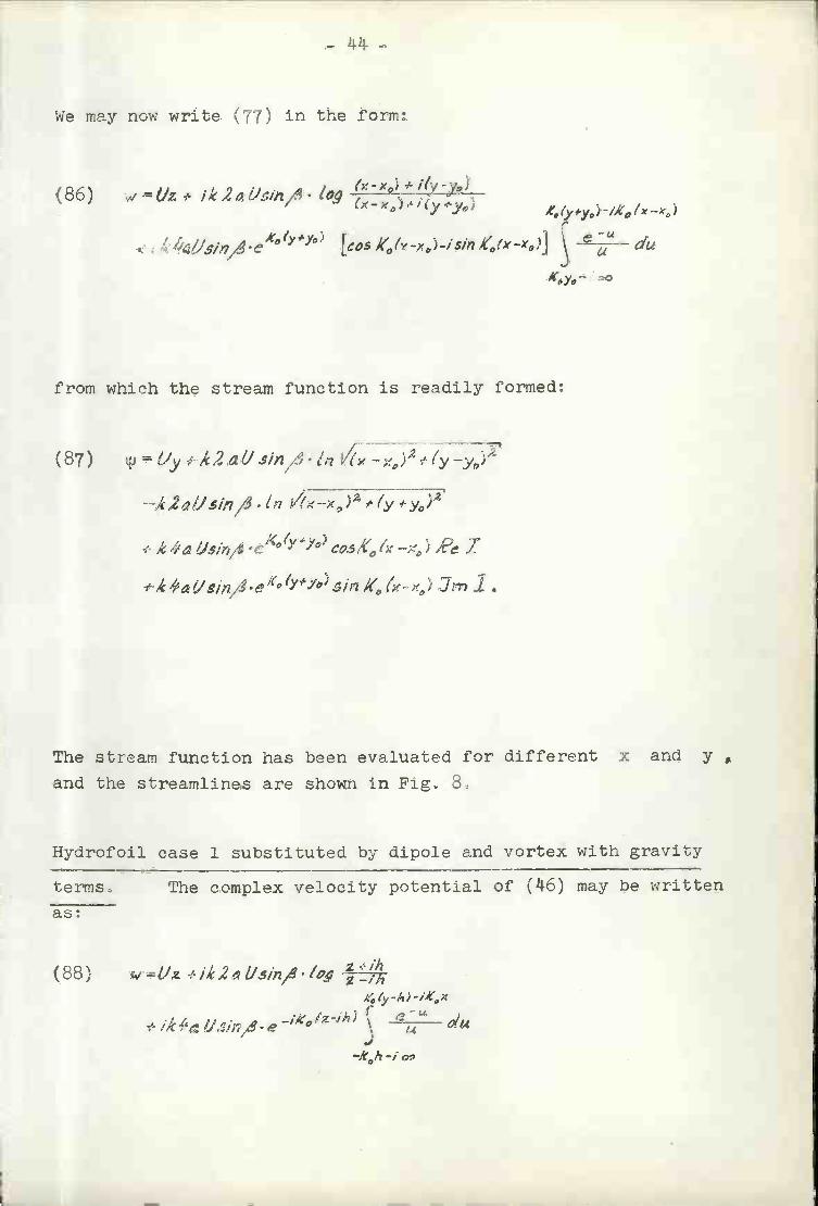
We may now write (77) in the form:
from which the stream function is readily formed:
2aJin,i3.tn
4'a ¿ls/ríA o'Yo CO'I': xa) .7
4ai,A.e1Y'Y0in/4(x) .7ml
The stream function has been evaluated for different x and y
and the streamlines are shown in FigS 8.
Hydrofoil case i substituted by dipole and vortex with gravity
terms The complex velocity potential of (24.6) may be written
as:
w=LJz/k2lJsÌn./og4 (y Á) - /4Ç
¡k - Ç
(86) \JUz ¡k2alIein/. log (?'-x0 í('yy0
4(y*y iK0/x.-x)
iJ$in/. 4 (y #y,)[cos A'-x0-i5/fl (r_X)] du
- 145 -
* a2_2eM0C) /J2_I2eiA'OC)
S
e a'u
-X0h -,00
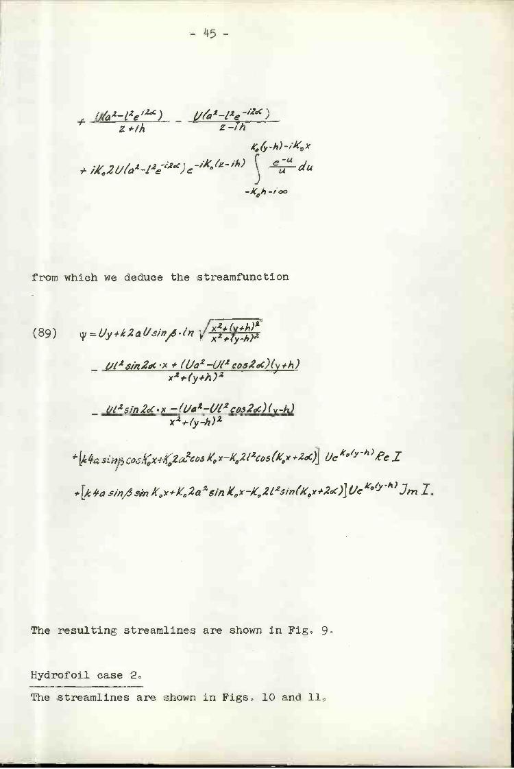
from which we deduce the streamfunction
z*ih 2-112
The streamlines are shown in Figs lo and iL
(89) =Uy142a1Lci17./n x2,' (h)2
-x # (¼2 U/2 cos2oc) (y #12)
x2*(y#h)2
¿'125m2c.X(y-h)
fr4. Srìf3CO.5Ax"Za.2(.OS k, x X,2 /2CO5(Ç #2oc)] ¿Je 'e» ee I
#/Ika sIn,,in /{o#Ko2a6in X0x-K 212s1n(Kx#2o4Je"0")Jpn I.
The resulting streamlines are shown in Fig 9
Hydrofoil case
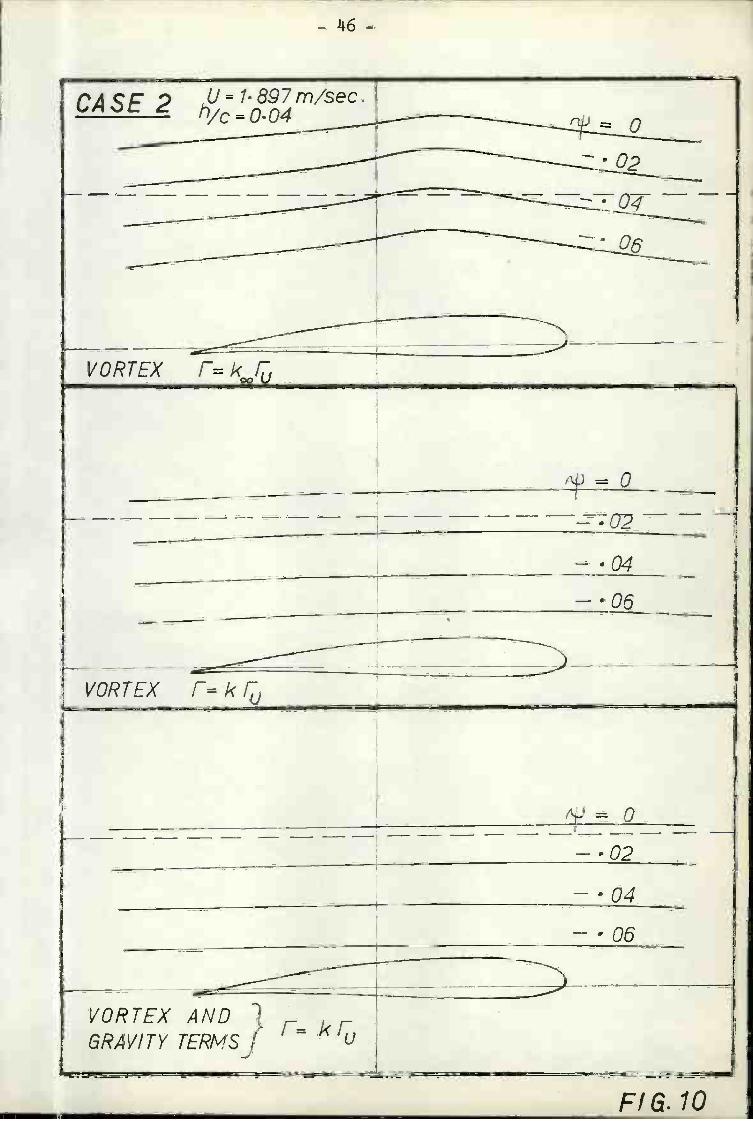
FIG. lo
CASE 2 U=1897m/sec.h/c0.04
'O2
-----o---VORTEX
AQ
0406
VORTEX rkr
02p0406
VORTEX AND R.
GRAVITY TERMSJr=
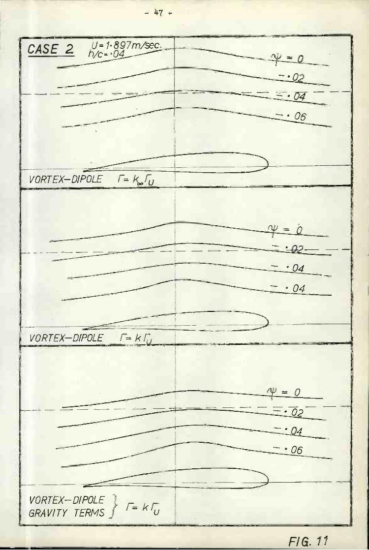
FIG. 11
CASE 2 U=1897m/sec.
-04 - -
VORTEXDIPOLE r Içr
VORTEXDIPOLE =kfi,
O2
VORTEXDIPOLEGRA VI T Y TERMS
r k
H
or, with
and
C
(91) - ¿i */v k / y(x)dx * /Ç
¡Y'x) dx
j xi-x j-i-i2A ITo o
-
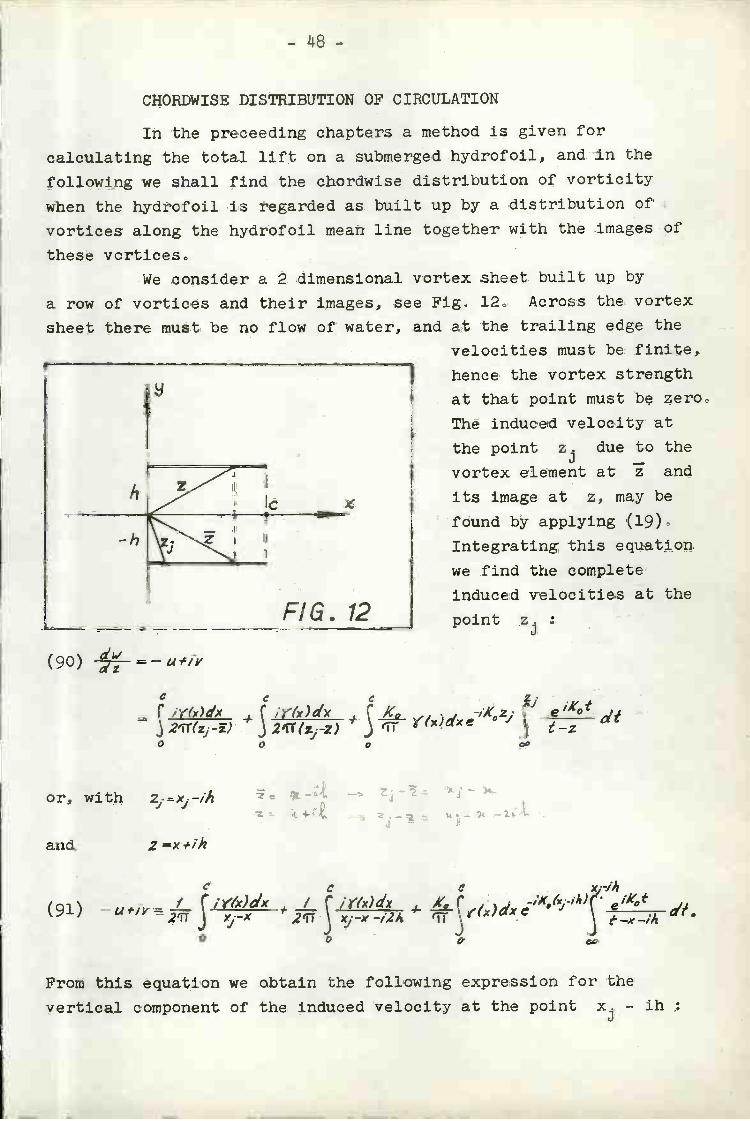
CHORDWISE DISTRIBUTION OF CIRCULATION
In the preceeding chapters a method is given for
calculating the total lift on a submerged hydrofoil, and in the
following we shall find the chordwise distribution of vorticity
when the hydrofoil is regarded as built up by a distribution of
vortices along the hydrofoil mean line together with the images of
these vort1ces
We consider a 2 dimensional vortex sheet built up by
a row of vortices and their images, see Fig. l2. Across the vortex
sheet there must be no flow of water, and at the trailing edge the
velocities must be finite,
hence the vortex strength
at that point must be zero
The induced velocity at
the point z due to the
I
vortex element at and
i Iits image at z, may be
-.
f dund by applying (l9).Z Integrating this equation
we find the complete
induced velocities at the
FIG. 12 point z.
(90) -=-avv
o C C z.r /Y(x)d.'c C ¡r()d +
a't2'rr(z -i) j 2 ( -z) Y (x ) dxz1 Ç e 1K0 t
o 0 0 00
>4-
o x-1i5
y () dx''T
di'.
From this equation we obtain the following expression for the
vertical component of the induced velocity at the point x - 1h
k9-
C C C Çe't(92)
L.Çr&a'x /= 2/ri 2 j (jx)2 4hz .Çr(x)a'x .Jm [ex(-i(x.-i4)J dt
o o O cG
or, with X0(e-x-/Á)A,
c c C
/ Ç Yfx)dx . j. Cr(x)(x.-xg'x() v1 - X 2TJ ()2 V(x)dx .JmfrxLiK.óv4Jt4-dÀJ
O O O oo-th,h
IntroducIng
(9k) x = f(/co )
jai--(/CO59j) cy c-- c'
we may write (93) in the following form:
Ir (Ir
(95) v,1 Çy(p)s/npd _L( ç)(co-cosçjsinp 4f2'rrj co p-coi ç1 2fT (cos-cos» #.(4ih)o o
e P dp Jm f (ces ip - ces1erTo -
Regarding the circulation distribution, we shall make the f ollowir
assumption which is wellknown from airfoil theory:
//-cA1p 4LJA ./n ,np*
satisfying the condition
i(0) O.

where
Hence:
(98)
- 50
Since there shall be no transport of water across the vortex sheet,
we must satisfy the condition (see f.ex [i4J)
(97) ,
çiuk e-
angle between foil chord and tangent to vortex
sheet at point zj
= angle between U and foil chord (incidence)
IT IT
i-o(-=4S/-osq d'f-co -cos
Applying the integral formula
IT
COSn'fCOStqCosLq1
efl.
(I- os r côsIT j (eos t CO5 p7) # (4' .4'-)
00z.A sinnwsi>npdqn.t ¿7
COS q -cas
IT
*sFr) (co -co»2 (42L)2
o
ir&2 j'/-ca5tP)a'LrJm [exflL_/Ahncoo6ije__a'Al
J
Ir 4hJ(CO5p-COSf)-i2k0h
;LAÇh -2X0h ,4sin n q' 5/n p 4 mFxp{IItchß(cw -° dÀ
à
5/fl q'.,. J Cf - C4.
:0
-
I, o
jL 't-

together with the relation
sin n 'p s/n ip =f{cos(n-/)p- ca
the two first integrals in (98) are readily integrated We find:
(99)
¿ I Ç 4srnn If $/ %9 = -2 I i,, Ca.5 Pl 9j.(loo)i-r
\cos-cos1
o
It is convenient to write (98) in a more compressed form by use
of the following parametre:
A0 C = -A0Co.54-ca5f1o
AhMJ -/24,h
i-r ke2 Jm(exL-/4',h
JÇe/ dAj
Qa-ìIt;#4
o
Introducing the notation:
iT
IT
o/mp a'p.
where
(102) = cos i - cas
and hence:
IT
(lo)) -Z,1-0c
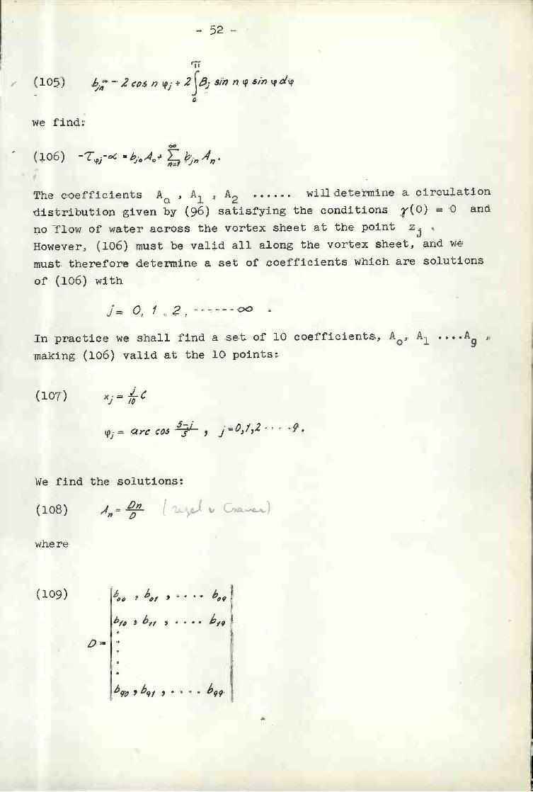
(105) 4;- 2 co n + 2jj si» n in a4
we find:
- (106) - -o = A0 ¿ .4,.
The coefficients A0 , A1 , A2 will determine a circulation
distribution given by (96) satisfying the conditions 1(0) = O and
no flow of water across the vortex sheet at the point Zj
However, (106) must be valid all along the vortex sheet, and we
must therefore determine a set of coefficients which are solutions
of (106) with
j= 0,12, ------
In practice we shall find a set of 10 coefficients, A0, A1 ....A9
making (106) valid at the 10 points:
(109)
D
= rc COS5;i , = O, 1,2-. -9.
We find the solutions:
(108) A - I 2c1LJn-D
where
470 ,46/ ,..-.....
- 52
, .. 499
(107) xi = C
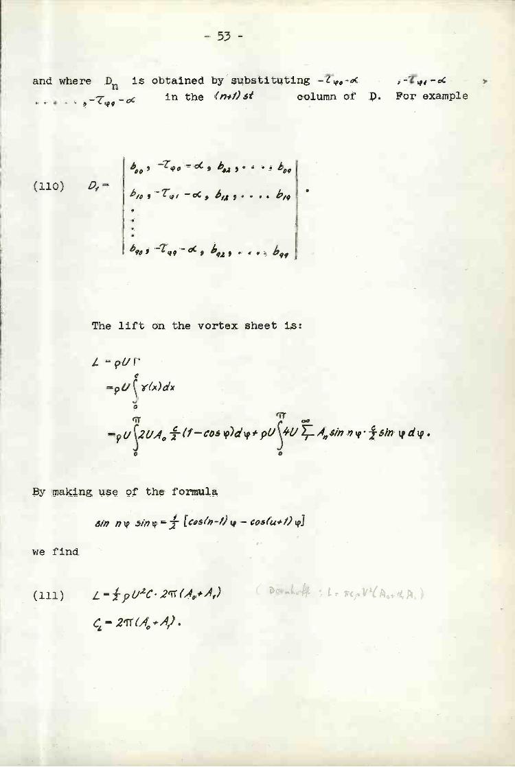
and where is obtained by substituting -T,,-(
-t-c in the (n#/)5t column of D. For example
- 53 -
"fl' .b00
- - c , . . . b,9t
b9, -7;, - oC"92
The lift on the vortex sheet is:
i =9ír=p1J5(9dx
.pli 21A0 pdp.o o
By making use of the formula
rn n w 5m (p = ;f (cos ( -1) L - cos # ,) pl
we find
(iii) LfpO2C2'iT('4o#4)
2'1TM,#4).
t
L:)
51. -
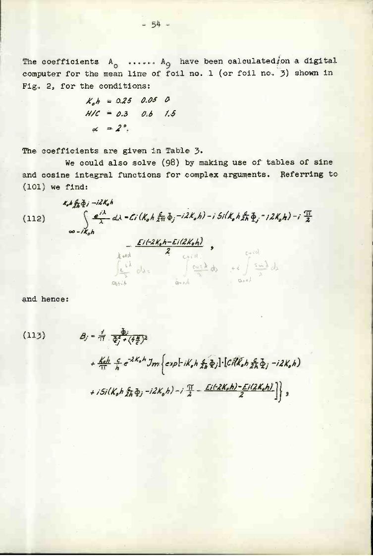
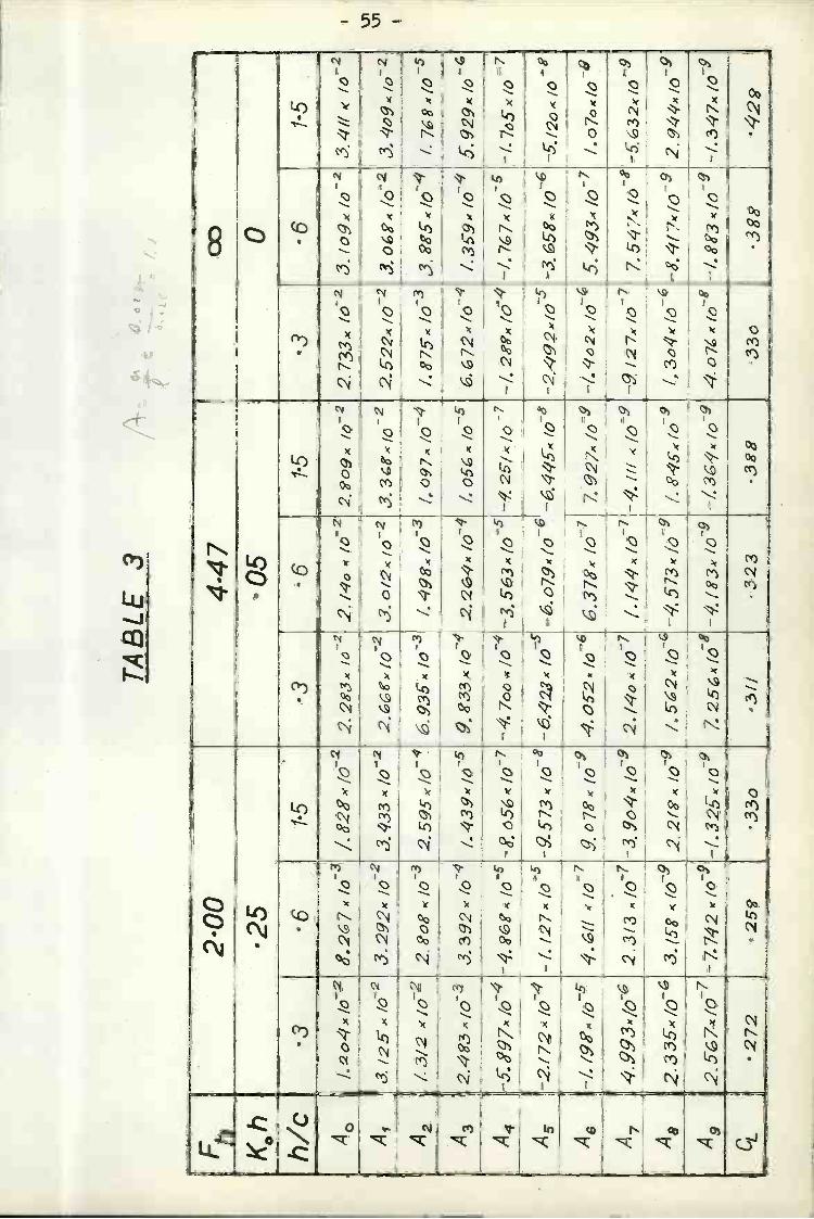
The coefficients A0 A9 have been caiculatedjon a digital
computer for the mean line of foil no. i (or foil no. 3) shown in
Fig. 2, for the conditions:
oC =2°.
The coefficients are given in Table 3.We could also solve (98) by making use of tables of sine
and cosine Integrai functions for complex arguments. Referring to
(loi) we find:
(112)S
EÀ dÀ -it4 -; 5iA/. -244) -0o
and hence:
(,(-2kh-L/(2k,4)2
a>
. 4jÁ f e21<°1Jm {exIiki4h4JF[C4'Á4A4j -J2Kh)
. ¡5/(K0hñJ -/2AÇ4') ,. y -2Ah)-4i(2.th) P2 .iJ'
A'Qh = 0.25 ¿.01 0H/C = 0.3 ¿'.6 1.6
TA
BLE
39
- -o
- -
h/c
153
-515
-3-6
1-5
A0
Jo4b
o8.
27x/
O3/
828/
02 2
.283
x2 2
.14o
*102
2o9x
iò2
2.73
3x1O
2310
9xb0
2 34
/1k
1O
A1
3.12
5x10
2 3.
292x
,o2
3433
2.%
fO2
3. O
/2x/
O33
/02
222x
/O2
ìo2
309x
ío6.
93g
m io
i./O
f. O
7 /0
I. 57
io3,
9S
5 /O
i, 7
g ¡o
A2
7.3/
2/2
2. o
8 Jo
2.59
5 io
A3
2.43
fO3.
392
1. 4
39x/
O5
9 33
x fÒ
2.24
x /o
I. O
5/O
.72
x-4
/.39x
I05.
929
x Io
A4
-97/
oIo
- ó5
f°-4
.7oc
3.56
3f0
2/x/
0_/
. 25/
O7ô
5x10
7
A5
-2./7
2x /O
-7. ¡
27 ¡
c-g
.573
1o8
-64
2x1S
-.o7
x70
6.4x
fO2.
492x
(O.5
5x /O
5.f2
ôx /0
A6
-/.8
o4.
fÌo7
8fo
4.2x
/ô6
6,37
8/O
7.g2
7A/O
/.ô2x
/O5g
<f7
/.o7o
1O
A7
4.99
3/o
2.31
3 to
-3.9
o4/o
2./4
ôx10
7 //4
4/7
-iíi /
ô9/
27/c
754;
1x/O
'32K
IO/.&
2fO
4.57
3/ô
/.R45
/ô/.3
o41ô
-8.4
f?/o
2.94
4/o
A9
2.33
x/O
3.15
8fO
2.2(
Io
4/83
10_/
34%
f0g
4.07
xfô
/.53f
O-/
.347
/0A
925
7/0
-7.7
42f0
-(.3
210
7251
OC
L-2
7225
330
-311
323
.33
330
388
200
4.47
2505
- 56 -
97
/1(/-CO?) tj(ilk) 6= jZ #(4 _»ZO
e2f(/ co )1e5/(4hhj"i244)Jm Û(A1,2Áh)(j7 ho
- co (JcÇh f,i ) d,
"iK0h c 21(h\(/..c05ç0)LJ?fl11h
o
EÍ-24'04) -E,/2K04) Js/n(Á'Dk -;)dLp2
i-r
c 24k* e -cod )E-,& 5i(-K +iÁh) Im C/(-Jh 24,J «,!KD 4)
tj
_frrrj
K0h c 24h- --e p))Jìn
t9j
-2Ah)-(2kh)]51(_,2
and
i-r» W S/I?(115) 4»-2eo n 4
O
± 'ir hn EEe C$/aÁÂ #;2Ç4) 2m C/(Á11 ,z *)
_]CO3 (k;,h j- 1)dtp
- 57 -
,h - ern n ip4srn wLJm Si(k,4fr1 #iZ4),'k'eC/(K,%2j #,'4 A)
o
(;(-2KÇ)-L7(2k'04) }smoc'04 frcj)d2
ir2t'4 e26Aj'irn n 'ç -c/n Eieesi(-#t hA ; #/ %4)#17m',(Kh f /2k, h)
-fr!1 côs(#t,h f1)d,
'Tr
2K,#Ç fe2t'1Çrn n q5fn /2kh)#&C/%j1,I244)"J
-2
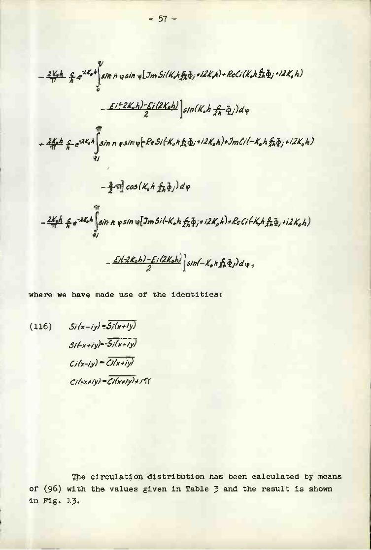
where we have made use of the Identities:
(116)
Sì(-x /y)* Siór#iy)
C'x-iy) - C/tx vyi
C//-xtiy) - ''iy)' ¡IT
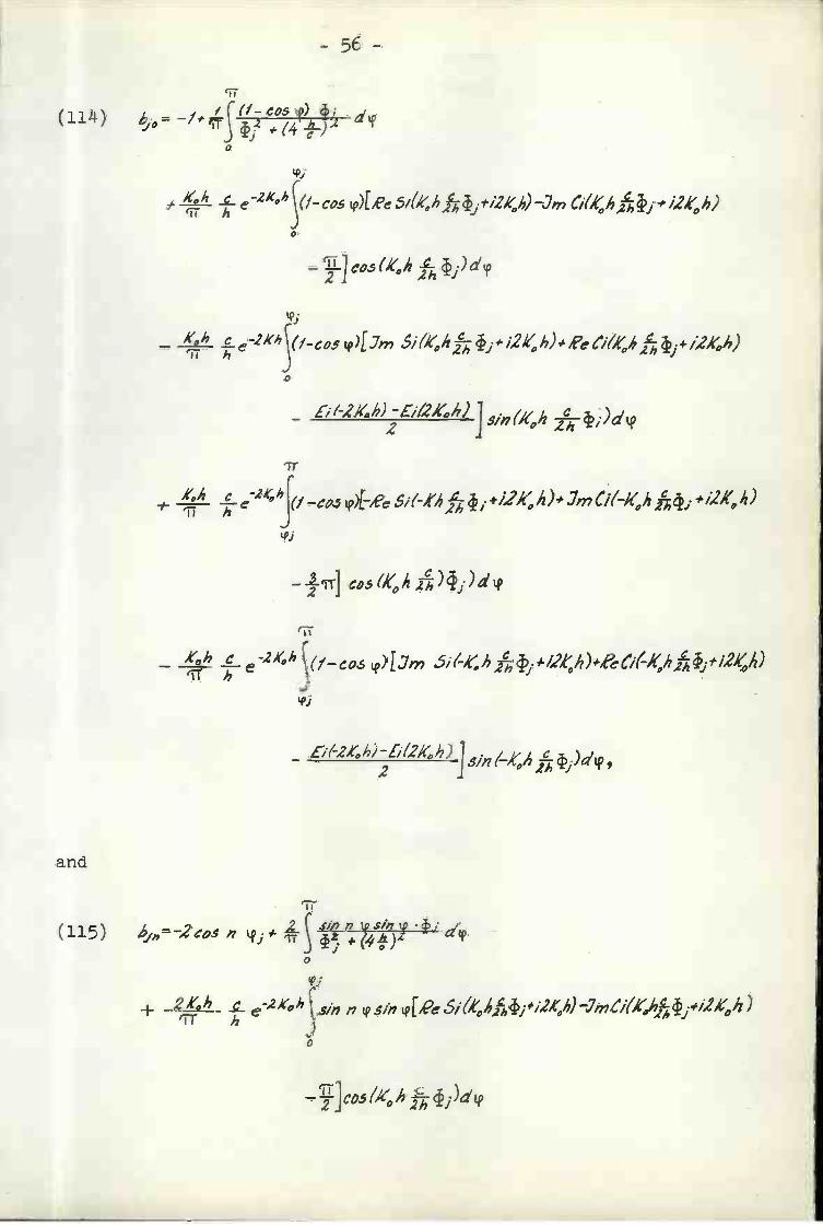
The circulation distribution has been calculated by means
of (96) with the values given in Table 3 and the result is shown
in Fig. 13.

- 58 -
FIG. 13
-I
.3
U
.1
o0
3
1 2 3 4 5 6 7 89 10
2
= 4. 4, 7
h/;±..
i - ---
0
/0
3
1 2 3 4 5 6 7 8.9 10
2
f=2
0O 1 2 34 56 7 8.9 10
- 59 -
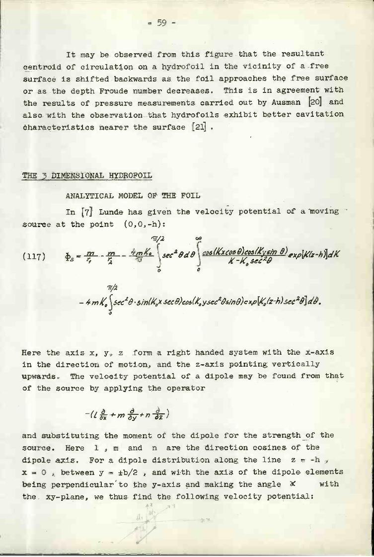
It may be observed from this figure that the resultant
centroid of circulation on a hydrofoil in the vicinity of a free
surface is shifted backwards as the foil approaches the free surface
or as the depth Froude number decreases. This is in agreement with
the results of pressure measurements carried out by Ausman [20] and
also with the observation that hydrofoils exhibit better cavitation
characteristics nearer the surface 1211
THE 3 DIMENSIONAL HYDROFOIL
ANALYTICAL MODEL OF THE FOIL
In [7] Lunde has given the velocity potential of a moving
source at the point (0,0,-h):
41/2
Lsec2 Odû ' ° ¶;» 8)ex4K(zh)1dK(117) A'-1sec
o O
- m K 6/fl(1CX ec8)cos(Ayxc2&s,»O)ex'1á (z -h) ec28J d&.o
Here the axis x, y, z form a right handed system with the x-axis
in the direction of motion, and the z-axis pointing vertically
upwards. The velocity potential of a dipole may be found from that
of the source by applying the operator
(t'-m ò-
and substituting the moment of the dipole for the strength of the
source. Here J. , ni and n are the direction cosines of the
dipole axis. For a dipole distribution along the line z = -h
x = O , between y = ±b/2 , and with the axis of the dipole elements
being perpendicularto the y-axis and making the angle X with
the xy-plane, we thus find the following velocity potential:

(1l8)
.6/2
xco.#í'z,.4)th IJ
1T/2
Sec
- 60 -
X CO5 zWz-h)5m z I N7,)&4r îT
b/Z
sìKxca8)caEK(y-)sth G3e.L K/i-I2 )1 co KdJK-Çsec29
Cú6(KxCt5 9)c'oLK/y-)s/i1ex,vIK(z-h)L;ìz z1C'dK
6/2 tTr/2
'kif Çft()d sec cs ( x cc )cak (y-ec20 ,
-6/2
.6/2 1V2
K02 1ft/&d Çc.si (K, xseco)csL x0 (y-) 5ec20 8]exp[&-h) ec9J5' dO.
-.6/2
The velocity potential of a vortex distribution along the line
z = -h , x = O , between y = * b/2, including the trailing vortex
system, has been given by Wu in 181
(119) (yzh)2 1 [x2#(y?)2#(z#)2t/2]d?-ill,
- 61
6/2
zh Ç r(y-7)2(z-h)2
[/# [X2#(Y)2(2h)t]/d7
- -i'- r( )th2 d Jec2ed9 coo (Á'.cs & Li'(y-r),,' 9] cx, [k(z-h)lic'dK.(- , sec2cÎrj
-b/2 o p
b/2
4 r()dpScos[#t'e'y)] exp[4ë(2-h)} d1t'
-b/2 O
b/2 91/2
- çs(kxe-4V2
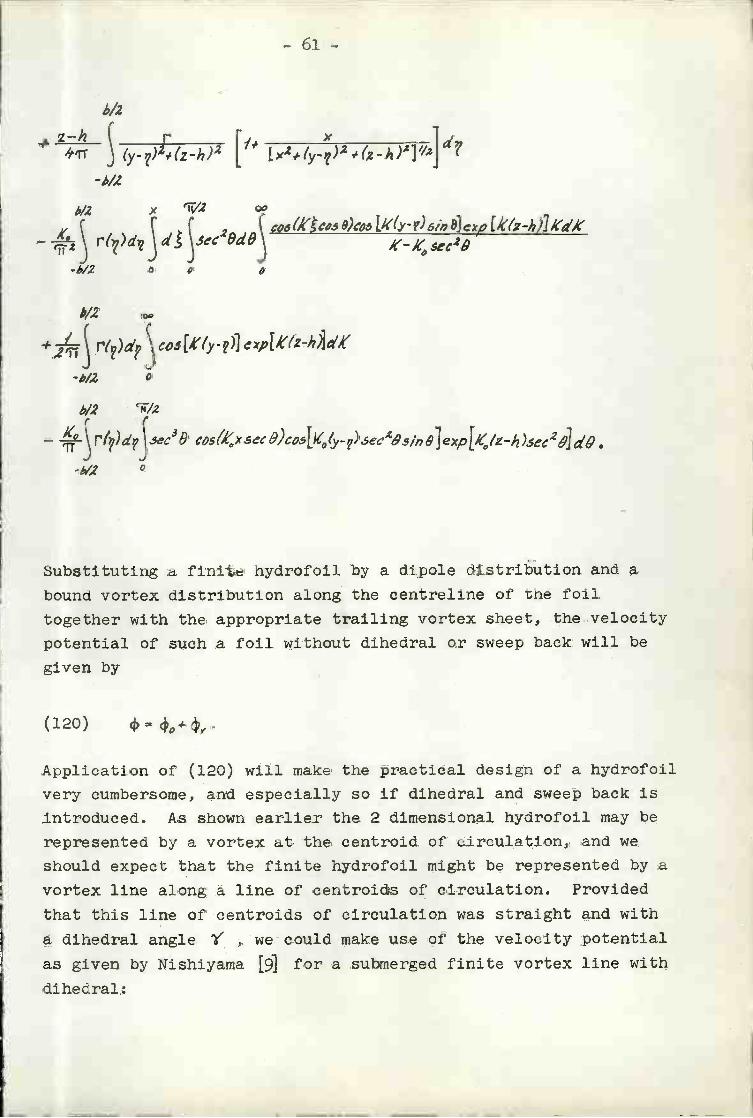
Substituting a finite hydrofoil by a dipole distribution and a
bound vortex distribution along the centreline of the foil
together with the appropriate trailing vortex sheet, the velocity
potential of such a foil without dihedral or sweep back will be
given by
(120)
Applìcation of (120) will make the practical design of a hydrofoil
very cumbersome, and especially so if dihedral and sweep back Is
introduced. As shown earlier the 2 dimensional hydrofoil may be
represented by a vortex at the centroid of circulation, and we
should expect that the finite hydrofoil might be represented by a
vortex line along a line of centroids of circulation. Provided
that this line of centroids of circulatïon was straight and with
a dihedral angle ' we could make use of the velocity potential
as given by Nishlyama [9] for a submerged finite vortex line with
dihedral:
b/2 X
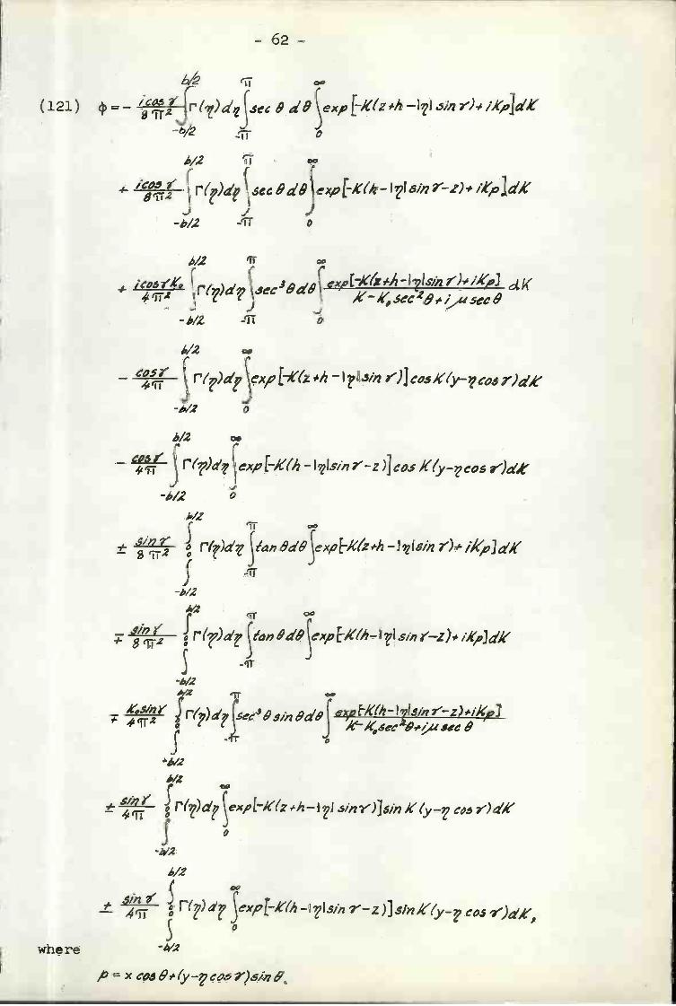
(121)
- ß2 j (r)deee8d8eok(_116mt)4to]dK-b/2 JT o
-b/2'TT
A'?7Y ¡r(912 7'
$
iT
89T2J ()dÇse 84' aSexp {-íc(z #h - 1J ia r) /Kp}dKb/2
62 -
OC
I ep&K(h- I 1Ism Y-z)#/1'pJkAec
$/i?V_ç00
±(IT
r()a'p expL/'(z 'h - i l 3/frVY)JS/>? K c r)dKo
-4/2
6/2
S/a '
o
where -4'2
p x
4/2 00
6/2 lT 00
dKjCD5 y4 1r()a'ec 38a'81X-% Se( 28 84972
-WZ tiT o
4/2 00
(05V 1( )dpexfl Et'(z h -1 3,>? y)] os frt'(y-rr
-A'2 o
-Is/n Y-Z)}J K(y-ces Y)d
4,/2
± r()déan 8d8expEk(zi'h - Ile/>z r)# i/(pJdK
J
.9/121'8'1r2
s
rr(?)d éa 8d8exp&K(h- ) l

Thin and deeply submerged hydrofoils with dihedral, might
be substituted by (121) when 'Y and h in (121) were replaced by
the hydrofoil dihedral angle and submergence at the centre of the
hydrofoil. Referring to the previous discussion of 2 dimensional
hydrofoils, such a substitution is doubtful for hydrofoils of some
thickness and with a small submergence, and moreover the practical
design or analysis of a hydrofoil would be very cumbersome by
application of (121). We shall therefore make use of a simpler
analytical model of the foil based on the results obtained earlier
for the infinite foil and which lends itself for practical applica-
ti on.
A usual assumption in ordinary airfoil work is to
substitute the finite wing by 2 dimensional strips and with the
wing followed by a trailing vortex sheet. The lift force on such
a 2 dimensional strip is found from the 2 dimensional lift
characteristics of the section when the induced velocity components
from the other strips and the trailing vortex sheet have been
added to the free stream velocity.
The velocity potential as given by Wu for a submerged
3 dimensional vortex without dihedral or sweep back, has been
discussed by Kaplan, Breslin and Jacobs [lO'J . They were able to
show that at high speed the potential approaches that of a vortex
and its biplane image when x is small (near the foil) and that
of a vortex and its wall image at large distance downstream.
Since we are interested in finding the liftcharacteristics
of the foil, or the down-wash velocity at the foil, we shall make
the assumption that the foil is built up by a series of
2 dimensional strips whose lift characteristics are found by means
of the results derived earlier for the 2 dimensional hydrofoil.
Further we assume that the hydrofoil is followed by a trailing
vortex sheet and its biplane image. For the application of the
results obtained for the 2 dimensional hydrofoil, we shall find
the corresponding moment of the 3 dimensional dipole distribution.
MOMENT OF DIPOLE DISTRIBUTION
The velocity potential of an element of a 3 dimensional
dipole distribution along the y-axis is (see Fig. lu):
(122) d //JCOÔZdJWr2
- 63 -
-
4 ç- J c
('.'S t

I / ò/j.a3 ,
= H.smrdy
The component of dv along the x-axis is:
4,.5mz
with a negative direction. The radial velocity component is:
ò '4'3
= /fcoZdy2íT3
The component of dv along the x-axis is:
CO5 't
hence the total velocity along the x-axis due to the dipole
element M3dy is:
- 64 -
and the tangential velocity due to this dipole:

and
- 65 -
= ,% Z a'y ra2L-3 rrr3
We further observe that
21 =
ay i- C062t
hence:
(2c v-srn'rcor)dr
Integrating we find the total velocity along the x-axis at the
point (R, O):
vTv
(2co3 z-5m2Z
m/z
When is considered constant, we find:
,32TT/?2MJ
The corresponding velocity due to a 2 dimensional dipole of
moment M2 is
y2!'2 2íi,c2
- 66 -
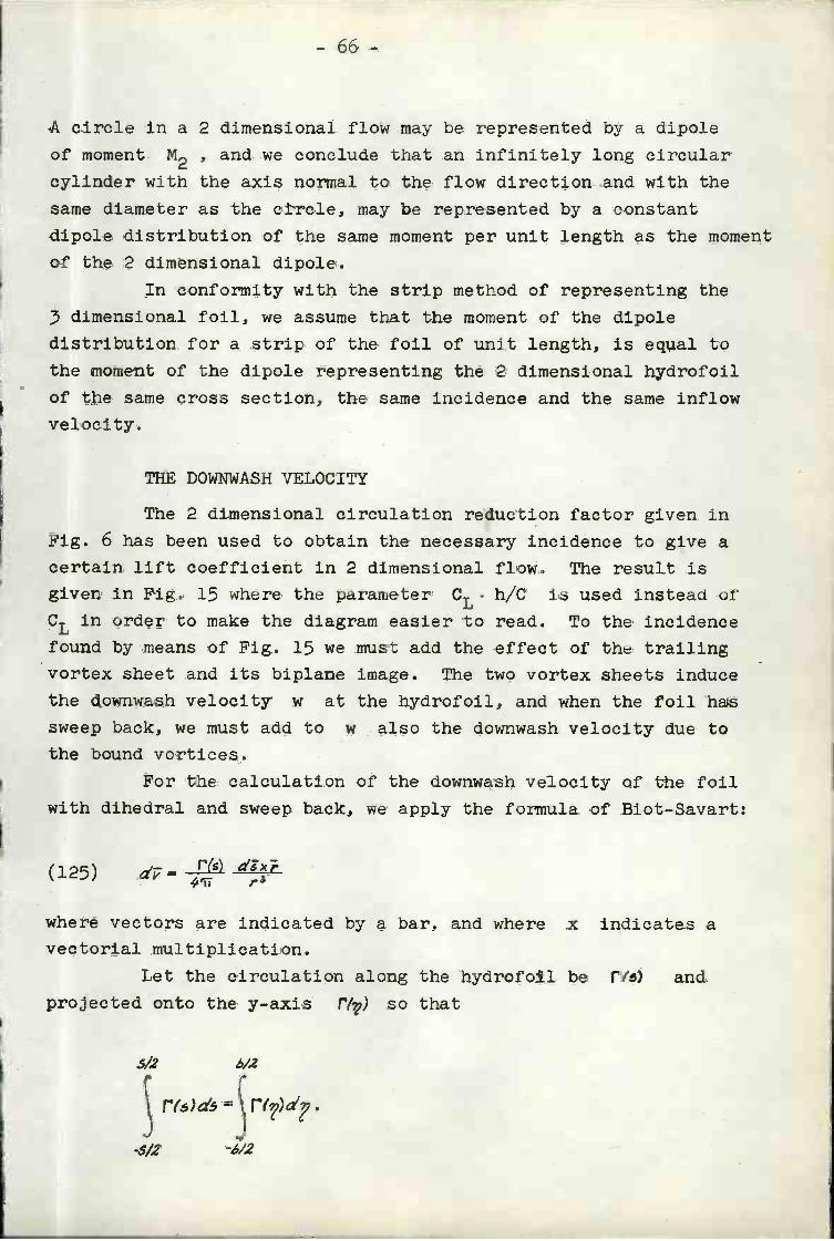
A circle in a 2 dimensional flow may be represented by a dipole
of moment M2 , and we conclude that an infinitely long circular
cylinder with the axis normal to the flow direction and with the
same diameter as the circle, may be represented by a constant
dipole distribution of the same moment per unit length as the moment
of the 2 dimensional dipole.
In conformity with the strip method of representing the
3 dimensional foil, we assume that the moment of the dipole
distribution for a strip of the foil of unit length, is equal to
the moment of the dipole representing the 2 dimensional hydrofoil
of the same cross section, the same incidence and the same inflow
velocity.
THE DOWNWASH VELOCITY
The 2 dimensional circulation reduction factor given in
Fig. 6 has been used to obtain the necessary incidence to give a
certain lift coefficient in 2 dimensional flow. The result is
given in Fig. 15 where the parameter CL h/C is used instead of
CL in order to make the diagram easier to read. To the incidence
found by means of Fig. 15 we must add the effect of the trailing
vortex sheet and its biplane image. The two vortex sheets induce
the downwash velocity w at the hydrofoil, and when the foil has
sweep back, we must add to w also the downwash velocity due to
the bound vortices.
For the calculation of the downwash velocity of the foil
with dihedral and sweep back, we apply the formula of Biot-Savart:
(125) r(s)9T r3
where vectors are indicated by a bar, and where x indicates a
vectorial multiplication.
Let the circulation along the hydrofoil be r(5) and
projected onto the y-axis rl,» so that
s/2
Sr(s)d5=r(?)dF.-5/2 -6/2

.. :::
::::::
::::::
:::..
ù..J
...:.:
.:U
...p.
Ub.
.....
1_
::':
L9::.
uj..
..F
....
: ::
L:
..:
JLJj
i4h3
:F .:
Wh1
hIJ
'$F
J!P
....
.¶!
. ....
.:il::
::::u
::2#I
.....
...ifl
:r.'-
.... :
!!u:q
:::...
......
.:::::
:::r
:::::q
::::r
::h.
g.r
g:rir
" r:
:::
L:::
L1
:r
aua
..:..n
..u'J
i:::q
:::..
....fl
. ....
.. s.
.._
. :L.
.....:
....
..:18
UR
. rn
#:::
::ll
"il
L.Lr
n:L.
.Lr
::pr9
dJj.:
..s
. .;.h
;.uI;;
;;r
Yg
z1f
r. ::
1jr.
...r
i.:!:
:j9k!
!:Ig
%5!
9hz
:P f
::
:r
::9g
:gg'
....
...:z
zmr
:::u:
::::::
::w:m
u;:.
...m
!.....
. ii!!
R..
-r-R
.!
:L!
:VØ
!!.!ç
..ij
j..!
.:::z
zu::
u::
; ir:
:::..
'z:
:::ir
h::::
::..
z:::
- 68 -
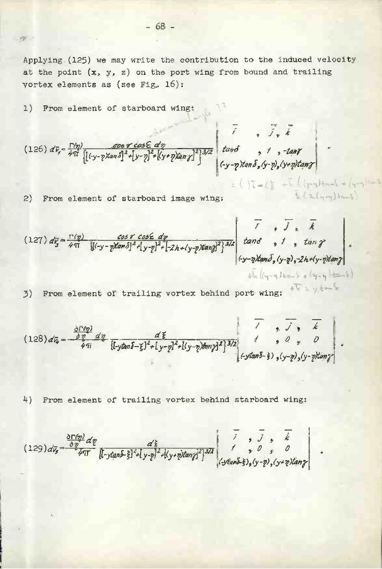
Applying (125) we may write the contribution to the induced velocity
at the point (X, y, z) on the port wing from bound and trailing
vortex elements as (see Fige 16):
i) From element of starboard wing:
j,A(126) 4 = 'rr f[ S 24y- J2#jy# rJ2j
3/2
From element of starboard image wing:
I ,j,(l27)dv=' r() rc
Q/76 / ' .
(-y-')tj, (y-e) ,-2h1'(y- ')irn
From element of trailing vortex behind port wing:
ò d{[-ytanî-J2* Ly_12*L(y_)t712}3/2
ò). '2)3/2(129 ) a'i = ')wnj j
, / ,
(-y-,)Qft5, &-'),&')a#rïL
/ 7/ ,c, O
(-ytm-- ) ,(yi),'yiXm;'
k) From element of trailing vortex behind starboard wing:
7' ,o , a
(-ytp$.), ( -),(y#&anT
.

- 69 -
FIG. 16

- 70 -
5) From element of trailing vortex behind port image wing:
ÒP(V(l30)d è., c17
4i1 {f-yi*nJ- Ly_12#[-2y#Fr?l312J312
6) From element of trailing vortex behind starboard image wing:
t1)a42
(131 ) d3=' 4cr
j ,j, T7' 0
(-yt4P S- ),(yi),24 (yq)vT
/ ,j, 4/ ,0, O
(-y4nS-V ,(y-)j2h -)6vi
From (126) through (131) we deduce the following
expression for the downwash velocity at the point (x, y, z) of
the port wing:o
Z '1)
o
(132) Ç2T j ty_p);]2#Lyij2(y)tì2J3'2-A'2
o
C5fcO tôìiSy I2Tr
Ja(_Y) JJ2fty_,J2,.[_2,4 (y_)t,nJ2JJi
4'12 -o.
Ç('Y ,)orb)d-à 'z ) ([-jtQoã_}32#Ty,12#L(y _,)tu32jsI2
o
n -
- - ) 4 [[y.J )2 ) 3/2

6/2
-k (y-) òr) d]2 [-2 h ¿y 3/2
o -?'-oc
/- a
-4/2
- 71 -
When y+ , integration of the last term of the k double
integrals will give:
o
cas
J )2#t,f '1y - ,)2,L(y#r)2,,>JJ/2
-4/2
o
Ct.CO5ttP1J.0 \2 îJ-
J[( a12d;(yi)2#L_2A#(y?)?,7l2}J/4
-,2
6/2
' / çÒr),,1
Yf#toé'ta#7) i#nj t' 1'
(1)3) w-

6/2
-h5&
4/2
(l2) _L.a?/çjft TJ
t,
- 72 -
a r (ag)/J)») {t(rp2t4J y-
ï
y
e
teìn J-fr('- 1 #(7)2 2hy)fr7ça)1 --Wi
When the foil has no sweep back, i.e. ¿ O , we have:
1
- TJ
,,' (o
o
Iri )T/ y1-liz
)I,!t24 )21
oIf tj-b/2
òr(

and when the angle of sweep back as well as the angle of dihedral
are zero, i.e, S r = O , we have:
6/2
/(135) w-
The last expression is the usual one for the downwash velocity
of biplane wings, and a similar expression may be found f.ex in
[1k]
DESIGN OF A HYDROFOIL
By means of the foregoing expressions, calculation of the
downwash velocity is straight forward when the circulation
distribution is given. Analysing a given wing under given flow
conditions is more difficult, but may be performed by successive
approximations.
For the experimental check of the strip method of
representing the 3 dimensional hydrofoil, we shall design a hydro-
foil for the following conditions:
speed of advance 6 rn/sec
sweep back 00
odihedral angle 15
total lift 12 kg
circulation distribution clliptic
draught at centre oo6 ¡n
foil span O.32 m
foil chord at centre 0-10 m
chord distribution elliptic
thickness/corde ratio 0.11 = constant
- 73 -

FIG. 17
- 75 -
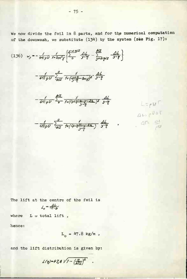
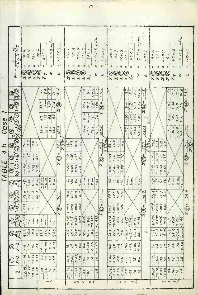
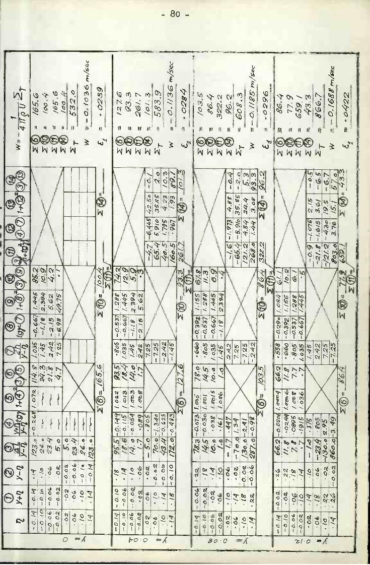
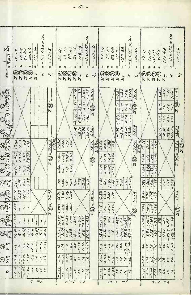
We now divide the foil in 8 parts, and for the numerical computation
of the downwash, we substitute (134) by the system (see Fig. 17):
(136)
where L = total lift
hence:
a/ '¼
rr2v 'b/2 f*(
6/2/ :5-Q /(/YFt2 )2 y
/ >° I ¿IL49Tp(1 -6/2 /(Qf) y-.
The lift at the centre of the foil is
9-r-b
L0 = 47.8 kg/rn
1/2¿iL ¿iL
and the lift distribution is given by:
(3)2
e
Lr

p'2.
av 0V
-4 .1=
7
.-
o. 9
8.4
-ô./.
'q-o
.i-q
.i4-0
.10
-&.1
Öfe
'
-o.o
1= -
O.o
.4o
-D02
-O
.02
QO
-02
.10
-'4 -o.ii
/ -o.
iô /8
-O. (
o -&
O6.
/4r
-o,o
1= -
CO
Q*
fo-O
.0.
OQ
Ö
-Oj
-0.0
4 .
-O.0
-0.
02. f
-0.Ö
(oó
_f-4
-0.0
2 O
1062
-fo
Ot,
-oz
-fo
.g -
o.o
(42Z
-O
.Ö?
O.O
-06
ÖQ
ò6(0
-O.o
2L/
1,n
.(-/
40.
Ö6'
fO
./25
(4/8
-0.1
03f
(-o
.4ê3
51/
35H
Z
- 26
.o
4(6
5.27
-0.6
73 '.
;-/4
.r-0
.03o
1..o
-IO
3/.1
5,,j
I.1J2
(o/.Z
:.4 7
1.31
.2.4
/-O
g
I(=
ô3.
5
'-C
.Ç'
I.1.
20-o
.c1.
/.ß7
-'-7e
,4.
a-t_
OD
-.7
3 3ö
I=J
.,7-o
.4o
/.f.
/5_I
.I&,
-O.g
9/.ç
:Z±
(.2-
o -O
.93
/87
t,-f
73 4
.0-V
.5,0
-t,.
-
TA
BLE
4a
Des
ign
1®1b
755_
f
S
.2/4
.34
7;.o 75
-ç
f1. o
Ç,2
.,2f
-f2.
'23
e'.o
-4.
.2.7
IQI.3
,-'
29r-
-72.
.I.
e2do
'..)
i@2=
77.''
-w.z
-1.
5534
'-7
.1=
2290
-4.
t'.7
_10.
g,4ç
3.7
35.0
-4q-
.1bz
2.o4
'5(.
0
I.Ct,
f(7.
Ç1o
7g'
4ff.f
23Ç
f.5F
3
(o. ô
v-
-co
-7&
-4.3
/ 472
Id)=
74J0
iW
_4T
TS,
UT
I I I I Iw =
-_
i. i
'ó5
h-1
= = = =o
=/4
/3/.
g
W=
- O
.(g(
o r7
/,
w = =
w
= .0
3/3
I©=
:?47
-. O
(4
-z'
í1.
-002
f. r4
/.2I
.-0
.10
0z22
44.1
o 24
41?
7.s
OS
9S27
.1-O
.OQ
/0¡4
II. Z
(oj
.14
.10
/&.6
37S
II06
19
-o"
-20
5.9
5IO
ÖQ
-2j
/4-
-0.0
215
7f -
3.49
q.E
-ö.
ii5.7
-4q.
-ô.0
54 f.
Ot3
4'q.
:24
089
/.dò8
'2.
8-7
hR
o5
.jtg7
12i
Y-'?
.-0
.2f0
722/
f.-'
---_
-.9o
.5--
---
7&.
7.3,
'Ó2
-O.0
.-0
1=-0
.ö6
.10
(4 -
0/4
Y-1
2'2
Y+
'2
=ic
g= 3
tE
h
f
- 0J
'f.
0713
3.2
-67
-040
I-/f
oS
h-c
$/.3
Ç-c
).93
/.?7
212.
!=
:2J-
/-.f
4Ç/.o
¿=
-03/
¿=
031
Ic
Eo
-o 0
2'Ö
2Ó
2 T
±°
.0(0
Ó, -
O.0
)38
.4.f
.10
-O(c
350
(4(4
-0/4
94
o ( o ç)
O. k
jj- o
. k?
-0. i
oj_o
. (o
02 66 10 (4
YQ 0(0
-0.0
(0-
O.O
QO
Q
-O
TJ°
-O.Ó
(,O
2.-0
0gO
,Io
0(0
.14
o .g
.14
[.0.1
4 T
OÖ
[:0 .0
2-O
.o.o IO '/4
4 /8 /4 fo -02
(o-C
.o2
.74
-0'O
.g .-
ô./0
- oz
-Ö.9
z-0
.Oé
z5ô
.-0
.020
L2:Z
..f9
oz4'
qf
12.8
05'9
S/4
535
.19(
5
Y-'?
.'9
4.3
35.ô
3'.4
37. 6
73.5
5. o
©
- o.
. '-H
-o. i
lSo.
054
-089
-37.
S.9
05/1
5.0
-/.4
o59
.3 -
O..z
5-o
.49.
3
-O. ó
73-O
.Ö3o
038'
1,I
-15
.447
-//5
.b¡.
3417
5,o
-;.4
I22
oô
.7.5
'.37
5-3
'4 -
2o5
-175
.o95
L;Ö
.o -
3.49
1*®
2
-o.2
f. O
7
1 02
2
1(6
3? .7
35. g
35. o
=/9
1.5
7.9
q. 7
¡2.4
1(5)
= /3
2.ö
= Iò
.9/.o
tq5.
S/o
,/5
,9/.O
Dg
/2.7
j.036
5.2
y-I?
.-8
6t o -6.
-2.
- f.
'2eT
AB
LE 4
bC
ase
i
co 55
tgr-
Ø-o
9 /3
-0.9
3/87
-/73
4.O
V-5
.73
33.8
-0.2
4'1(
)7'
_Ö.6
9.1
¡3G
-°31
,7
- 64
e-S
G-0
.59
/35
/t.5
1.2e
_o.9
3/.g
7/2
.2c
v-i.
734c
v3.
/
9.4
/g/.
1(T
h=J
I
.7
-0/9
l.o36
9.o
-o.2
gi.o
7gi4
.&-O
,4o
1.16
/1.0
-c.5
9/.3
54.
c
/(
74Q
ÇO
.5
55.7
/2.2
4.0
3c.°
5,7
333
1.73
4irz
3:.7
.93
/.7g0
9 /.
35 I6?.
4
-351
0-5
.2o
'I -'
z.44
.,ó22
.75.
/&
53/.3
'Z
9/Q
c.-9
/23.
072
/G2
Rl.
o
2es.
o
2 9.
3
I
/. ô2
iE
.Z(1
d)=
'1
I. I
9.6
/g,.7
7e .o
(If.
2
1.8
-7o
O.2
¡.67
-4.5
-bT
S -
/.2o
2.44
-/5
7-I
G.'2
.P/ô
3-(
7.o
e(o
739O
516
4= L
3.3
iW
_4T
rSU
T
I L= =
/02.
91f
J=
1J =
IW-
0. ff
3/.&
QC
.
=
w=
-o.
iç7
w =
./O?/
--1/
c.N
¿=
.07
W ¿
=59
1_I
=52
.7s\
.L/
84.6
7' g
'.'-
o9. 9
53.3
26.
,
O3o
5
=/3
2.I
=97
.4I
=25
o.5
I=
/7/,2

o Il
12y+
1zy-
12
-o.,
-o.jö
/g-0
.06
/
OQ
-&I.1
-0.
04 z
-ojo
-&
OZ
.,g
-O.0
.O.
- f-
4-ô
.OQ
O(ô
-0. Ö
.
O-O
Z.1
4-0
6.g
,1'j
Z2
-/4
-
- oz
-0.0
-z-0
.0
Y-'?
.17
.23
-I7.
095
.9.
57.
03.
'17
.2
'34
1.2/
4.2
3.i7
9.27
-
--
OQ
-9.
5. P
o5-C
.o2
21.0
Ö.Ö
(D5.
,7 &
f.2S
-o-1
0 24
.! -o
.4S
3
10.9
5 -Ó
73¿
72 T
°°3°
:038
L9f-
1-3
_17
.447
-2/.o
1.34
/55_
-.2
.4I
4o-2
-O
.98
-0.0
20
-1.9
-37S
-04
-gp5
-0.2
. -16
.5.9
5-ô
öz 1
20.5
-3.
49
f. o7
-0.l-
4'f.O
-0.1
15 /.
013
-ö.o
54 f.
0b3
O89
f.O
-ò
16.c
s2.
896.
559.
8e
I©=
/747
- I.
2o-
o.
22.6
2
IO 9
e,1.
72
/.S5
JAB
LL 4
CC
ase
2
5 -o
.:ò7
1 /0
.15
-67
o.4o
1; /,
-86
059
¿g
2.22
/.Q.
25,7
r71o
2.
- 0.
19
Í48
1.03
689
5
293
_52o
28./-
0.34
.-4
p6 2
27-9
2¡.
382.
911.
7872
1.52
/5.S
S1'
.2/
_T?.
96 -
/.55
3.4
-O93
-i95
-466
22.
7 -
0.93
/445
1 y9
/3.9
1.12
37.5
óI-
022.
O4'
f974
I4)
19.c
o
-1.7
7 -.
042
/.e7
-'Li
-6.5
3 -/
.2o
2,44
' -22
7-/
445
-3 c
.Ç /0
.3 -
/.5o
/f2.2
o2.
577.
3 b
a63
89/5
=-/
2: I I
iW
_4T
TS
U T
=34
35/6
45=
34_3
5=
/6.4
5=
/01.
60w
O.O
39ffm
/(f
= O
/9'
I) T-
w ¿f
2: 2: 2:
22.'G
2/3
.23
3.5'
. 0E
/8-2
f95
./2=
-O
..037
m/6
= -
oies
-0/5
7/4
, g,
/328
89.4
5/1
. o 2
= /2
8.ô5
w=
- 0
,O5o
=. o
2g0
ori.
-22
1.41
-oz4
q-0
.28w
/0 t
1.3/
-0.0
6/9
0895
1. le
;-O
.OQ
IO14
1.36
-0.5
9 t:3
51-
o
= /6
.45
34.3
534
.35
w
=¡7
47
1) =
29.4
3=
/9,0
0=
So.
77=
-0.
03/m
/

T;?
-014
-0.
I'?-0
.10
-&.fc
-0.0
6 -o
.o.
-0.0
.2 -
O.0
202 06 fo (4
-0.0
4I_
0.10
O.0
2. .i -
o.c
OQ
-6.1
4-O
-IO
-0.0
6
Y+
'2Y
-12
10 14 ¡gÓ2
-Ô.0
.ô(
..1
0-0
.Io(4
-oi
l
"4 'fo
-CO
Q.
Z4
.02;
.2Z'JI
2Ç97
.oIö
7o.o
5gz
0. 2
.o
/ß9,
o38
.25
-o 5.0
.o--
.-f'
-0.0
2-/
0/4
3.6
ôZ14
io-5
.o-0
4-5
t.4.1
0o.
-35
0.o
/4O
.o20
8O.d
Y'T
f gy.
- 12
25o
534
-7o
.o29
7.
-O. 0
73-O
.03o
038
('I&
f'-4
47-/
75.4
'f.
35b.
o -,
4/53
o _ö
.qg
1-.c
-u2
/ô.o
-0.
02o
/.T4
3/.'
oz4
/.ßtIb
409
95i.c
r.r
1(S
[o36
375.
95m
3.
25&
8
2/4.
7
Q Y-1
2
277.
1.03
554
1.4
554
.5 2
4223
.37.
25
/88.
o38
.5'
8o2s
.o 1
.035
4'9
/.4'5
,-' 2
.Q2
7.25
'_7
.2.r
tg-Ç
7
667
/.'/4
5-/
18 í3
,4-
-2./Ç
5Z
-6.5
8 49
7Ç
-0.3
52-O
.53j
-1/8
'
2o /04
J5
24'6
./q2
o.2
'cm
=J
1.15
5/3
.31.
282
30.2
/445
/73
2.34
2.!
I©=
_2/3
.4 8
02.c
/o.
-55e
-42
9e/4
773/
.:.6
6e -
O-3
92 1
.15_
52z
5/9
.4 8
o5 -
& 5
37 /2
8:/5
.23.
5 ¡.
635
-67
1.44
6Q
.5'.4
52.
-42
7.25
-7Q
5
12
6/?'
4'5
¿'2
.j -0
e;5.
5'o
351
¡.Z
?54'
.23J
27.
0.97
/.73J
2/6.
oL
I=4'
7-9
-.9
-/97
3 4.
83-1
.7-/
3/-1
.9/ 3
5.8
-4.9
325
4.8-
4 Q
4.4
/4.4
_46
5 /4
4 3.
oe 2
25.ö
iQ=
232.
8
2T-4
'5 -
i. 6/
5 3.
61-1
6.2
27p-
43/2
.5 -
/8.c
/94o
.ó 3
.7c
13./
/38.
0LS
!I)
= /0
h5
I4T
Tç3
UT
I I w 1
="1
2o.2
= =4'
2o.2
= = /3
32.
0285
=-.
/875
'i/s.
=. 0
3/2
256.
82/
3.4
8c Q
. o23
2.8
T=
/505
.ow
= -
o./9
55/
= .0
326
I6)
= 2
147
=/9
2.9
= /5
53.8
=/o
/.5=
2O
2.9
W-Ò
.26c
?lfl/
SE
t
= .o
447
-o./q
-.0
.(0
-/8
¡.02
222
.o 8
o5 -
0.53
7 /8
/7.9
. S'
-0.1
0-O
.O'/4
50.o
-O
.!¡5
/.::'t
3',9
4/,0
35-û
.i7 /.
5 34
'.-
O.O
QIo
35.ø
-ö.
054
/.0b3
3«.y
J.4
'5'
-1./8
2.3.
9V/4
'.-0
.0.2
ÖQ
O8.
q08
9 /.ô
gg4
2.4
2 -2
.15'
3-62
/..5
.02
06oz
-25
.o o
57.
25-2
5.3
Ô6
(o-O
.62Z
I75.
o-/.4
,í!
.°/4
//65-
0.62
5-2
.q2
/o8.
á(4
¡g-0
.10
4/.o
-o.4
338
&o
- o
f. 07
2
I©=
318
.7Q
ç=_2
4'O
.23
I=
3/8.
7=
27a-
2
247.
Y=
Q Il
û /''
-o.i
o-0
.0-',
Ö2
Ob (o (4
Y'Z
Y-1
2
-O.k
/ -o.
14.4 ¡g /4 Io
06O
Zfo
-0.6
2/4
-O
.00'
-18
-ot
-OJ
-0.O
42.
Z-ö
.tc -
o.o
. fg
-0.0
6O
Q-
-O.Ö
__ O
i;,IO
o
y-ri
/43.
0
23/
5_. o
783
/45
fo. 1.ô
ytg
Y-1
2-
O.2
23.4
'
/23
.-
-5:0
.o5
7c.o
-/.
34"
43.1
/ -'0
. tzS
172-
o -o
.43
-0. ó
73-O
.O3o
038
.Oz
-04
.14
-z -
7o.c
L34
.g-4
±2'
7.o
_ô,q
g
1.i.®
f. O
7Z
/6.S
965-
o.'--
r Iô
.z93
.5/8
.6-O
. 11J
3 J8
..4'
14.
-c 0
54 f.
T3
/4,o
1.7
û89
¡.0?
&1.
7
/27.
.6
7g'.o
&G
o -0
,39
¡.15
567
.gI.
ÔD
(¡4
.5P
805
_O.5
37I.
288
/1.3
f.rc1
5/0
-oI.o
35 -
0.Ç
,7 1
.445
6.9
/O2.
é/.d
1.45
' .-1
.l'2.
39-4
.4
Ic=
/03.
5Z
,66
.2 -
0.02
of.
-i-o4
-'6.1
0-
-22
II.--
--oz4
/ I'
-0.0
6¡'
7.F
O89
-6.0
2. l
o/4
.7 .(
9f5
¡.o6
./4
./-
/O.3
76'
-23.
4.
1ô2-
o -/
3&o
.95
/4-0
.02
860.
01-3
.49
/,4. g
'1.
036'
-O
(D7
¡.44
,524
.3¡.
45-(
./2.
394
/0.9
21.8
242-
2.15
5.2
4.2
7 7.
25 -
6.98
49.
75.
J
1.03
5-.
4524
27.
25-7
25-2
42
.2.4
.272
5-
725
-2.4
2
6.Q
.558
ii.: i
6o7.
7-8
o5.7
/.o35
1.45
2.42
7.25
-7.2
5
-0.5
37 ¡
.288
-0.6
k7 1
.445
-1.1
8.2
.394
-2.1
5 52
=
'(Th=
J74
.2/2
.9 5.9 .3-
=93
.2G
I i
-0.2
90 1
.084
6/. /
-0.3
92 1
.156
/0.2
-0.5
37 1
.288
¿. /
-O.7
1.4
45-5
322.
2
_-_4
.7 i_
5o -
C. /
65.4
9Io
36.8
52.
c4o
.3I.7
964.
23/0
./6
.5t
. 9'7
1.93
99. /
LZ.
/cI.3
-/.
-1.9
734.
88 -
0.4
-6.4
. -s.
910
355'
-2.
ó/2
/.24.
84' 2
4.4'
5:3
261.
o1.
443.
os 9
3.3
96.2
-0.9
-1.
075'
2.1
5-0
-Ç-2
1.1
-1.6
15-6
.5-/
2/.2
-43
19.5
' -.7
c?03
.o3.
76/5
.15'
7ô77
65P
./43
.3
I 1 I I IW_4
Uy
w-Ö
./036
m/s
ece1
=
/2 7
=93
.3=
26/
7/o
J.3
583.
9w
=-C
.//3G
n-t/s
ec=
.028
4'=
./0
3_5
=86
.4'
=32
2..2
=96
.260
8.3
w=
- O
. /f9
5 P
'i,1e
c
-.0
29e
77.9
65g
/=
.4.3
.386
6.7
w=
1=
-0.
4222
O
O.O
(.
-O.0
2
Io
0.Q
.O
.O 0.02 02
Ó2
ô( -io
-O.0
L-ö
.o&
II
- 4
14-o
.i-q
I=
/651
6z
/65.
G= =
532o
'2 02 66 (0 (4
-bill
-0.
04-Ö
0 -O
.ô.
-0.Ó
-OQ
0-0
2
10
() y+,
Y-'2
-0(0
/8-ô
..ö1
.14
O.O
Qfo
-02
06-0
2(o
-0.o
2-/
4O
.Ö9
-/8
-(°
Io-1
4 ¡g 2Z
O. O 02 IO
2, -22
y-ri
24. 5.'
4,7
L,O
4-O
/1.6
75.
,Q
4- 19.'
.3.3
-4.0 /4.o 85
34.-
4
Q -ö.0
54-0
89 905
-I. 3
4o-o
. 25
-o. 4
3
22/5
.6-0
.073
./g2.
e3-o
.03o
«1-4
2.o
-038
-Io
q' íi
.o-1
.33
«L.
-&-/
4,d
1,34
-0.O
z25
.5-2
,4/
-O.O
574
-ö.9
9
/3.:2
-o.
O2o
2.32
oz'
ìq/.5
3 -0
9S.5
7 i1
O.
-14
Io-O
.S37
-. /
O4
21
2C
.2. -
25.5
2.9
514
O02
/72.
0 -3
. 49
1®2
/ 072
I o.2
/.c'i3
/ . C
b 3
t O-Ò
g
23.
437
437
3.7»
.
= 3
5.88
I()=
2.4
fl.Ö
b/5
.53
/.ÔD
I2.
3!.a
-o(5
2.oø
/.0'é
7?
Z©
= 2
/./4
/ 3. 2
o2.
3Q/.5
4S
S
/76/
y-ri
/035
1.45
.242
7.25
/8.7
o'8
ô5J.
6o ¿
O35
2.79
1.45
¡.32
2.42
7.25
- 7.
25-
2Á2
-1.4
5
805
1.03
51.
452.
4272
5-7
.25
- 2.
42
.-0.
7 /4
45-I
-18
2.3q
4-2
.15
S.t2
--6.
98 4
9.7v
-9. 3
7-
O. 6
67
-1-/
es'
-2. /
S
a® / Zoo
2.13 83
/.2/4
.82
/44e
; 22.
394
1.17
5.62
.24
-0.3
9.2
1/5b
/.26'
82.
Qo
-1.1
923
94'
.33
558
-O.2
9' /.
ô4'
/6(
oo -
0.39
2I./
ST
Ç.2
°!.g
os -
6.53
7 12
8f¡.
2/I-
035-
-O
.7 /.
44.
'4/
52.
-42
225
-725
i
-.44
s .4
2.cc
-.c
.ö_f
o.9
'° 3
85.3
97
/79
4.23
2.0
/32
./e96
7/9
3 /7
85=
"5
4'9.
4/
I/3.5
.2
= /7
.44
63.ö
6
-0.7
5 -/
o7-4
.3-i(
a/5
-23.
êo -
4.3o
/6o.
53
.Th
/5.8
c/3
1.59
I(T
hf
-/24
' -1.
973
4..5
' -0.
27ig
r°23
9ö 4
..4 2
4.4
/.o&
53.6
o¡.
44'.
'/f.
621=
/9öi
w=
417
ÇU
=3S
'82ö
.o'
= 3
5S?
= =///
.84
= =/8
.75
1(17
) =
494i
2o./G
=1/
4.73
w=
-022
4
1 I 1 1 Iw=
-. o
.
ç =
-02
/8
u qe W=
0. O
47
m/c
¿02
351(
5) =
/7c'
//5
.11
) =
/3J.
59=
8.43
Wo6
7n7/
5cc
¿Ï
2/ /4
/744
63.O
/9,0
/=
/20.
65
= /7
3.-4
3
= .0
338
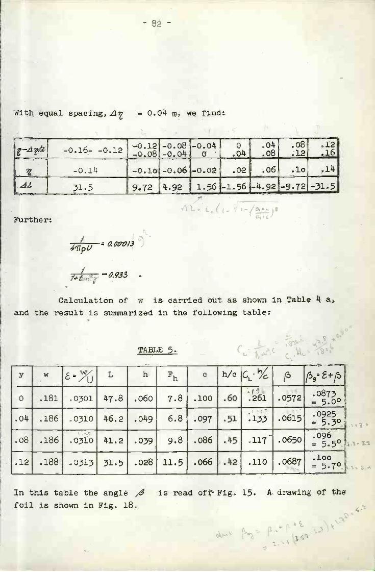
With equal spacing, Z17 = 0.04 m, we find:
2933
Calculation of w is carried out as shown in Table 4 a,
and the result is summarized in the following table:
- 82 -
TABLE 5.
f-Further:
In this table the angle ,4 is read off Fig. 15. A drawing of the
foil is shown in Fig. 18.
-i /z 0 16 0 1- . - - . 2 -0.08- -0.12-0.08-0.04
-0.04 00 -
.04.04.08
.08
.12.12.16
-0.14 -0.10 -0.06 -0.02 .02 .06 .10 .14
31.5 9.72 4.92 1.56 -1.56 -4.92 -9.72 -31.5
y w ¿ L h Fh c h/c CL i ¡
0 .181 030l 47.8 .060 7.8 .100 .60 .261 .0572 0850
.04 .186 .0310 46.2 .049 6.8 .097 .51 .133 .0615
.08 .186 .0310 41.2 .0)9 9.8 .086 .45 .117 .0650
.12 .188 .0313 31.5 .028 11.5 .066 .42 .110 .0687

- 83 -
Joukówski sectionsA aj 1mL= 23°
FIG. 18

8k
'NALYSIS OF A HYDROFOIL
As mentioned earlier, the lift distribution on a given
foil under given flow conditions may be found by successive
approximations. As an example we shall analyze the foil wh.L;h
was des1ned in tne foregoing chapter under the followingconditions.
'4k=50
U =km/sech = .06 m
o
The analysis is 'arried out following the steps:
Assume a value of E , called £ , equal to f.ex.
1/3 ,4g at centre of foil. This E value is kept
constant over the span.
b) Compu& fre) CL is found frort Fig. 15 and the Uft distribution
is 3omptted.
d) The first approximation to E , i.e. E iscalculated using Table k, and the procedure is repeated
with £2 =f(E0,)
1)
2)
speed of advance
th'augnt at centre
at centre
U
U
ni/sec
0.06 m50
=2m/sec= .06 m
50
3) U =6m/sec= .0725 m=50
U
h=km/sec= .0725 m
o=5
5) U
h=2m/sec= ,072 m
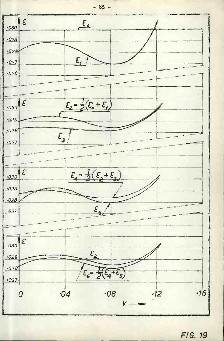
- 85 -
FIG. 19
030¡E o
029
02
027
026 -S_
'O28
027(3/
029
028
0274
,
0 '04 '08y
12 16
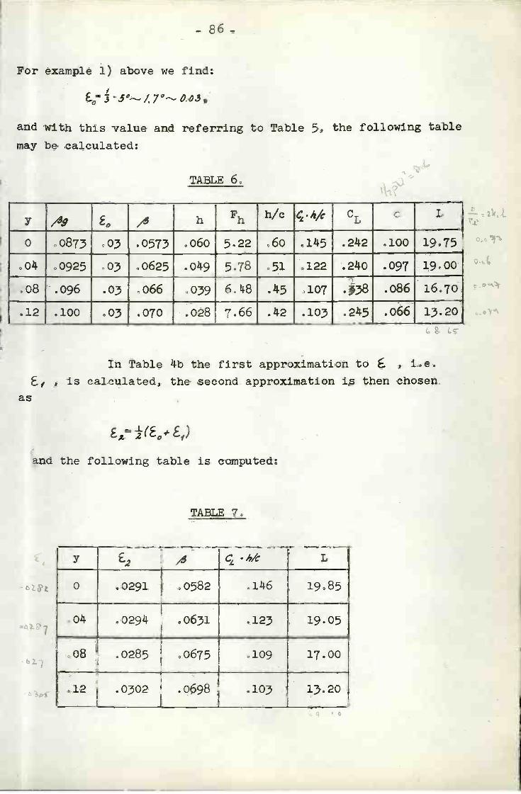
- 86 -
For example i) above we find:
and with this value and referring to Table 5, the following table
may be calculated:
TABLE 6.
In Table b the first approximation to , I.e.
is calculated, the second approximation is then chosen
as
£ ±(E0# E1)
and the following table is computed;
TABLE 7.
83:
a
OD
A h Fh h/c h/c CL L
o .0873 .03 .0573 .060 5.22 .60 .15 .22 .100 19.75
.0k .0925 M3 .0625 .0k9 5.78 .51 .122 .2k0 .097 19.00
.08 .096 .03 -066 o39 6.8 .k5 .107 .38 .086 16.70
.12 .100 .03 .070 .028 '.66 .k2 .103 .2k5 .066 13.20
y £2 Ç.4/c L
0 .0291 .0582 .1k6 19.85
.0k .02911. .0631 .123 19.05
.08 .0285 .0675 .109 17.00
.12 .0302 .0698 .103 13.20
- 87
Since only the lift distribution 4 L is altered,
a recalculation of Table 14b is very easily done, and a new
approximation to E is found. Once more this process is repeated
giving £5 values very close to the values, The E values
obtained in the different steps of the process are shown
graphically in Fig. 19, and it has obviously little meaning to
carry the process further than to the approximation E6 , where:
E= 'E,).As a matter of fact, a comparison between E and 6 shows
that even £2 will be accurate enough for practical purposes.
See the curves at the bottom of Fig. 19.
The analysis for example 2) through 6) above is
carried out similarly, and the calculated lift distributions are
shown in Fig. 20. The results of the analysis are given in
Table 8. Integrating the llftdistribution as given in Table 8
in the column headed L kg/rn, we find the total lift L kg, also
given in Table 8. Based on the submergence hrn and chord Cm
at y = 0.08 (= ), we may compute a mean submergence/chord
ratio (h/C)m and a mean depth Froude number, Fhmo These are
given in Table 8. The total lift based on mean depth Froude
number and as a function of mean submergence/chord ratio is given
in Fig. 20 for the design condition and the analyzed off design
conditions.
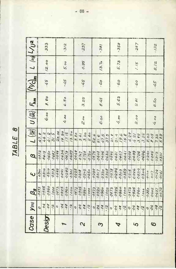
TA
BLE
8
Cas
e(m
)/3
/3L(i
m(h
,)L
(kL,
2(J
()
o0g
73. 0
:30/
P05
7247
. 9'
.04
'092
603
/o96
f54.
2D
esiç
r'.
o45
12.0
033
3o'
090
'Ö3f
o05
o41
.26.
12¡e
co03
/3O
69'7
3/ g
O08
73O
285
0588
2o.0
004
0925
'02/
'cn3
419
2e4c
c5o
o3/
208
O9G
ô'0
292
°78
1716
'/2'0
30/
Ö99
/3.2
oO
0873
'022
538
e
2ô4
'092
502
1307
o73/
2cc
3.25
.45-
o.9s
237
O90
'02e
2'07
5g3.
2e'/2
fOoo
'025
o'0
75e
2.G
oo
'087
3'0
299'
'057
552
.
304
0926
0317
./Qß
945
O/3
.7e
'38/
ogO
9Go
033o
'03G
47.5
'/2IO
oô'0
368
'02
37.5
oc2
973
'027
805
9521
.8,4
09g
.029
403
/21
.45.
3'0
5.73
358
'0g
O9Ç
oO
303
O65
7/2
'035
'906
41o
0?73
02/5
05#
4.2e
'04
09.2
5''O
22'0
699
4.2/
2oo
2.s/
o¡.
15-
'287
ôSO
90-0
234
'072
G3.
6'Q
'/2/o
O3c
4Ò
6932
gO
035o
-011
e'0
24e
o3
604
'040
2.0
117
029'
68.
O5
5ö-4
52.
72-1
32'8
.043
7'
'012
403
/3Z
33'/2
o472
.0/4
/.0
33/
589
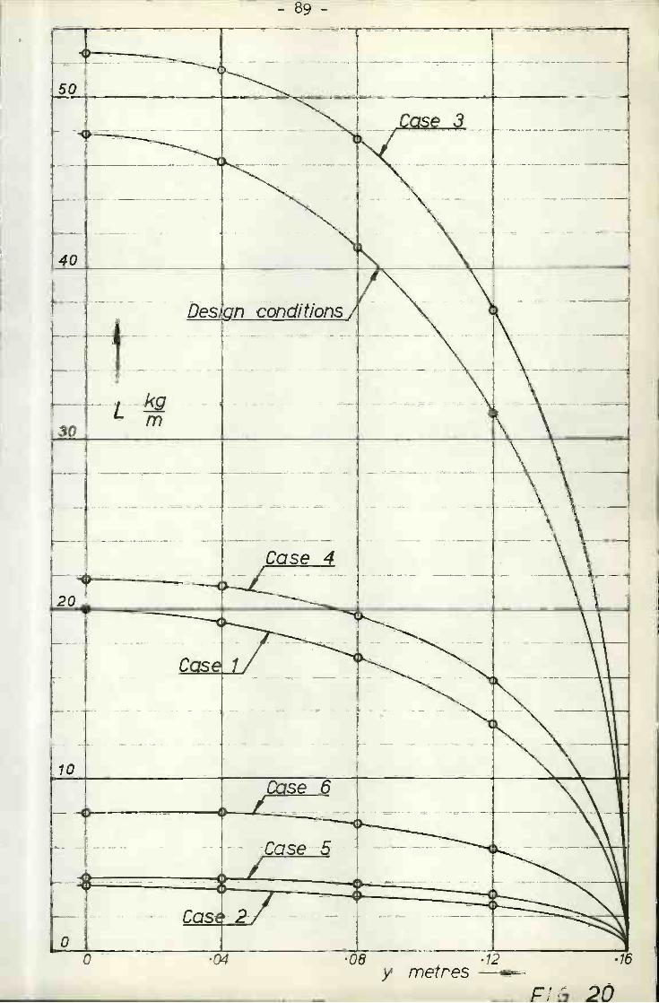
- 89 -
08 .12 16y metres
r1; 20
H
s-3
40
Design conditions
ï
20V.
Case 4p
C.sV
Case6/- oCase 5
2Cas-

EXPERIMENTAL PART
THE DYNAMOMETRE
A 6 component dynamometre siitable for general model
testing of hydrofoils, trawl boards, yachts, rudders etc was
designed and built, Some guiding principles for the design were:
i) The recordings should be based on electric strain
gauges in order to make the instrument as simple as
possible.
Component interferences should as far as possible
be avoided since separation of 6 components would make
the use of the instrument complicateth
The recording part of the instrument should be above
the water surface to avoid unnecessary disturbances
of the water flow and inaccuracies due to moist strain
gauges.
¿t) All forces and moments should be recorded directly
on the recording paper so that intermediate calcula-
tions could be avoided. It is f.ex possible to
measure a force norrrial to a bar by recording the
moments due to the force at two sections of the bar.
The force is then (N1-M2)/l, where M1 and M2 are
the two bending moments and I is the distance
between the sections. By recording the two moments
the force could be computed, but in connection with
f..ex. tests in waves, calculation of the force would
represent a considerable amount of work which should
be avoided.
5) There should be a linear relation between the forces
and moments and the recordings by the instrument. This
will simplify the analysis of the recording papers.
A drawing of the dynamometre is shown in Figs. 21 and
22. Vertical position of the foil as well as angle of heel, trim
and yaw can readily be adjusted. The possibility to alter longi-
tudinal or transverse position of the foil relatively to the
carriage was not considered to be of any importance. The recording

- 91 -
::SISI
a..
i
s.
I
u
s
Lift
---- --Side force
DraQ
Yawing moment
Pitchi i
i
Rolling u-
358
îr
- - - - - - - -
1
FIG. 21
tI - I

L
H L
'L
-
yuit
4
I
fi-
J- i
S SJ
IIT
L-
J -
I

Straingauges
- 93 -
Bridge
Connecting rod
Deflection plates
Bridge
Bottom piafe
r-
/f
¡I
II
FIG. 23
i H To pp i at e
- 9 -
of the 3 moments is straight forward; it might be observed that the
strain elements are connected to the fixed points by short rods to
avoid axial stresses (tension or compression) in the strain elements.
Due to deformations in the instrument, such stresses might otherwise
be very difficult to avoid.
In Fig. 23 is shown the principle of recording the drag force,
the same principle being used for recording lift and sideforces As
observed from the drawing the vertical deflection plates are made
thick and broad to reduce the unwanted deformations due to the
3 moments, the lift or the sideforce. At the same time the plates are
given horizontal notches at the top and bottom to increase the
sensitivity of the drag recording system and also in order to reduce
deformations of the horizontal top- and bottom plates. Further, to
obtain symmetrical and linear response and to avoid component inter-
ference, the strain element and the fixed point of the connecting rod
were both attached to bridges resting on the top- and bottom plates
at the connection points between these plates and the deflection
plates. The spherical bearings at the ends of the connection rods
for lift, drag and sideforce, were shrinked into the rods to eliminate
clearances in the roller bearings. These clearances amounted to
approximately 1/loo mm in a free bearing, which could not be tolerated.
The strain element and the bridge circuit are shown in
Fig. 23 With this circuit the effect of temperature is cancelled
out as long as the two gauges are subjected to the same temperature,
which may be expected for this instruments At the same time the
output potential is twice as great as when only one active gauge is
used The dimensions of the strain elements were chosen to give
bending stresses at the gauges from i - 10 kg/mm2 at normal ioads
Extensive calibration tests n the dynamometre, has with one
exception, shown no component interference The exception is the
drag recording element, where a trimming moment of 100 kgcm about the
drag element introduces a drag readin of 003 k. This seems to be
the result of a slight, initial inclination of the notched deflection
plates due to inaccuracies when welding together this part of the
instrument, When testing hydrofoils, the lift and drag forces will
give a resultant which usually acts through the drag recording element
Hence the trimming moment about this part will be small, and it is not
necessary to compensate for trimming moment influence on the drag
readings. Generally, however, the drag readings must be compensated
- 95 -
for trimming moment influence. Since this is the only component
interference the compensation is simple, but still the drag recording
part of the dynamometre should be replaced by a new part. It may be
noted that in a strain gauge balance, component interference seems to
be difficult to avoid and is often accepted [17] . In {18J is described
a 6 component strain gauge balance where each component influences all
the other components. Even when the interference is linear, it would
be very time consuming to calculate the separate components from the
readings in case such a calculation should be carried out by hand.
EXPERIMENTAL SET UP
In Fig. 18 and Fig. 2k are given details of the foil
arrangements.
The arrangement for measuring lift distribution on the
3 dimensional foil is best explained by Fig. 18. As shown one half
of the foil Is divided into k parts by slots starting 1 mm behind the
leading edge and 1 mm before the trailing edge. At the centreline
the slots form strain elements onto which strain gauges are glued.
Before and after the model tests, the system was calibrated by loading
the foil tip with hanging weights. The material left at the leading
and trailing edges at the slots served to absorbe torsional moments
so that the strain element left in the centre of the profile should
be exposed to pure bending.
2 DIMENSIONAL HYDROFOIL
The hydrofoil shown in Fig. 2k departs in several ways from
the theoretical 2 dimensional hydrofoil as treated earlier, and
differences between predicted and observed lift may, besides imperfect
theory, also be due to:
Effect of viscosity on angle of zero lift.
Effect of viscosity on slope of lift curve.
Boundary layers on the struts.
k) Flow contraction and increased speed due to wedge
shaped struts.
Flow circulation around the outer struts.
Lift forces on the struts.
Variation in lift due to effect of laminar -
turbulent flow.
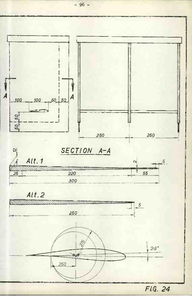
i25
Alt. i
Alt.2
bSECTION A-A
220
300
250
- 96 -
i250
C\1
55
250
FIG. 24
50HSO100
o

-97-
The effect of point 2) and 3) Is a reduced lift, whereas
the effect of point k) is ari increased lift. Based on data given In
L5J the lift reduction under point 2) may amount to approximately
2%. The effect mentioned tinder point 3) Is difficult to evaluate,
but the displacement thickness of the boundary layer, see f.ex.
[161, will give an Idea about this effect. The displacement thick-
ress for a laminar layer is
(137) 6= 1.73 / X
which, with x = 0.1 m , u = i rn/sec to 6 rn/sec, will give:
c(=0.2-0.5mm
According to data given in [16], the transition from laminar to
turbulent flow takec place at Ux/ = 300 000, so that we may
expect a laminar boundary layer on the struts upstream of the
foil. With a d1sp1aement thickness as given above, we therefore
conclude that the effect mentionea under point 3) will be
negligible. The increase in speed mentioned under point li.) is
difficuit to evaluate, but Lince the contraction amounts to
approximately 3%, it is expected that the increase in speed is
small. It Is therefore assumed that the effect of point k) more
or less cancels out the effects of point 2) and 3), and in-any
.ase these effects are too small to seriously disturb the
2 dimensional flow.
It is tiffIoult to determine whether there Is any
circulation around the outer struts as mentioned under point 5)
above. A series of test was therefore run with different
distances from the foil to the leading edge and to the bottom line
of the outer struts. The two types of outer struts are shown in
Fig. 2k. The main test series was run with the distance from
the leading edge of the foil to the ing edge of the struts
and from the foil to the bottom line of the struts equal to the
foil chord length, and the test series to determine the amount
of strut circulation was run with the distances above equal to
half the foil chord length, as shown with dotted lines on Fig. 2.
No differences In 1' could be detected, however, and It is

- 98 -
therefore assumed that the effect of strut circulation is
negligible0 After the main test series was finished, the struts
were run without foil and the lift was recorded0 The observed
lift value during the main tests were corrected for lift on the
struts and for buoyancy forces on foil and struts, and the
corrected values are given in Tables 9a through e.
Referring to the discussion above, we must expect that
the test results are to some degree disturbed by the presence of
the struts, by the effect of viscosity and by some 3 dimensional
effects0 In order to calculate the experimental circulation
reduction factors, k, we have therefore plotted the observed
L/1J2 values at constant Fh and ,c5 on a basis of h/c0 The
curves so obtained have been extended to give asymptotic values
of L/U2 at large submergence0 These values again have been
plotted at constant ,4 on a basis of depth Froudenumber to give
asymptotically the final values of L/U2 in unbounded flow,
Based on the values so obtained, the k-values in the
Tables 9a through e and In Figs0 25, 26 and 27 have been computed0
It may be observed that the agreement with the theoretical values
of the circulation reduction factor is satisfactory at h/c > o6and ,4 20. It is noted that ,,'ß = 20 corresponds to a
liftcoefficient less than 0.2 which may be regarded as small from
a practical point of view. At h/c = 033 and O»1 the agreement
with the theoretical values is less satisfactory0 It is
supposed that the main reason for this disagreement Is the
increase in submergence depth due to the wave formation above the
hydrofoil. The wave heights were observed during the tests, and
the result is given in Fig0 28. Based on these observations,
the theoretical circulation reduction factors have been corrected
as shown in Figs. 29 and 30, and also shown in Figs0 25, 26 and 27
As observed it now turns out to be a much better agreement between
theoretical and experimental k-values at the lower h/c values
where the submergence Increase is best felt.
As mentioned earlier the agreement between theoretical
and observed circulation reduction is best at the larger angles
of attack. This might have been expected since a certain
disagreement in angle of attack is best felt at a small lift or
small angle of attack.
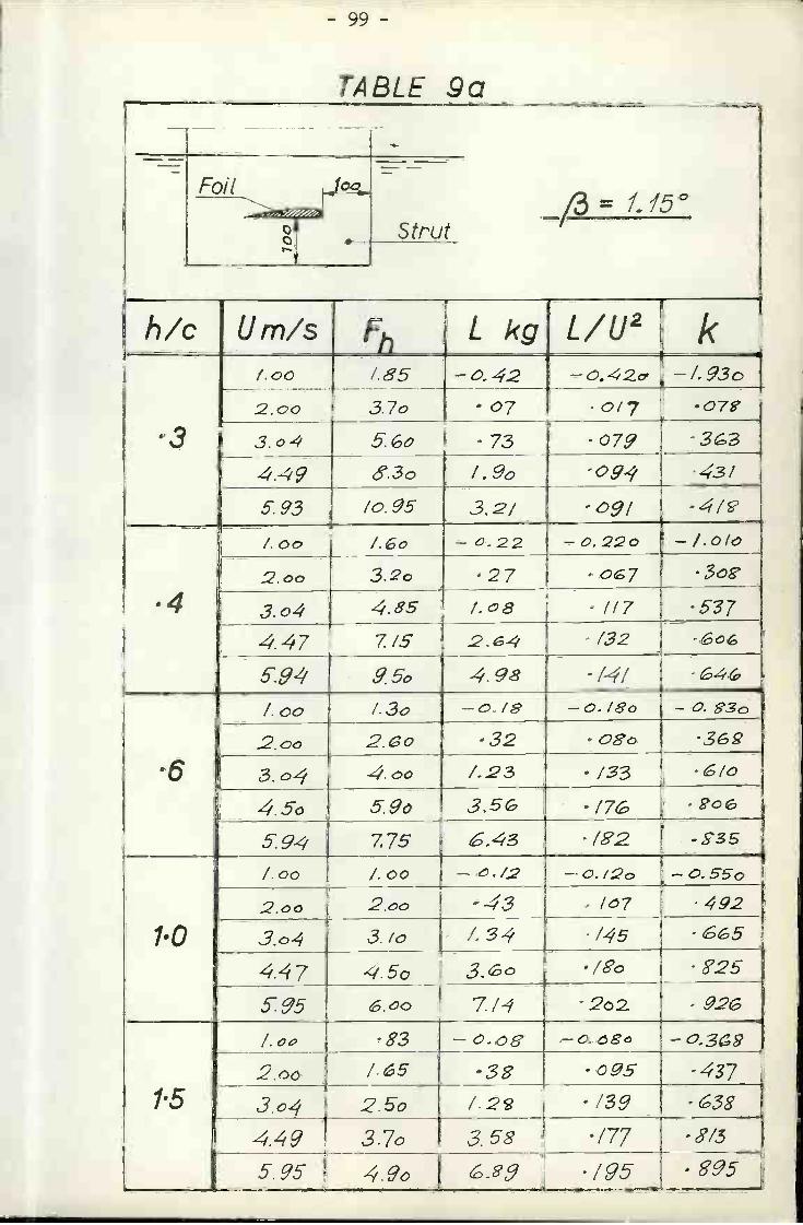
- 99 -
TABLE .ga
/3 = 71. 15°Fo/I loo
Strut
h/c Urn/s F, L kg k
.3
4
cY
3. o4 7
-. 47 .O
6 94
'6
I. cc . ¿. 0. 93
2.cc -. -369
3o44.50 - -
5:94
10
¡.00
2.co 492
3.o
47 3 ./'o3T95 7./- 2o2
15
/. 83 Ocq O.ogô2.ôo /.5 38 -005 -437
2.5o 7.2S -13g .3g4.49 3.7o 3.8 -177
5.95 4.9c // g
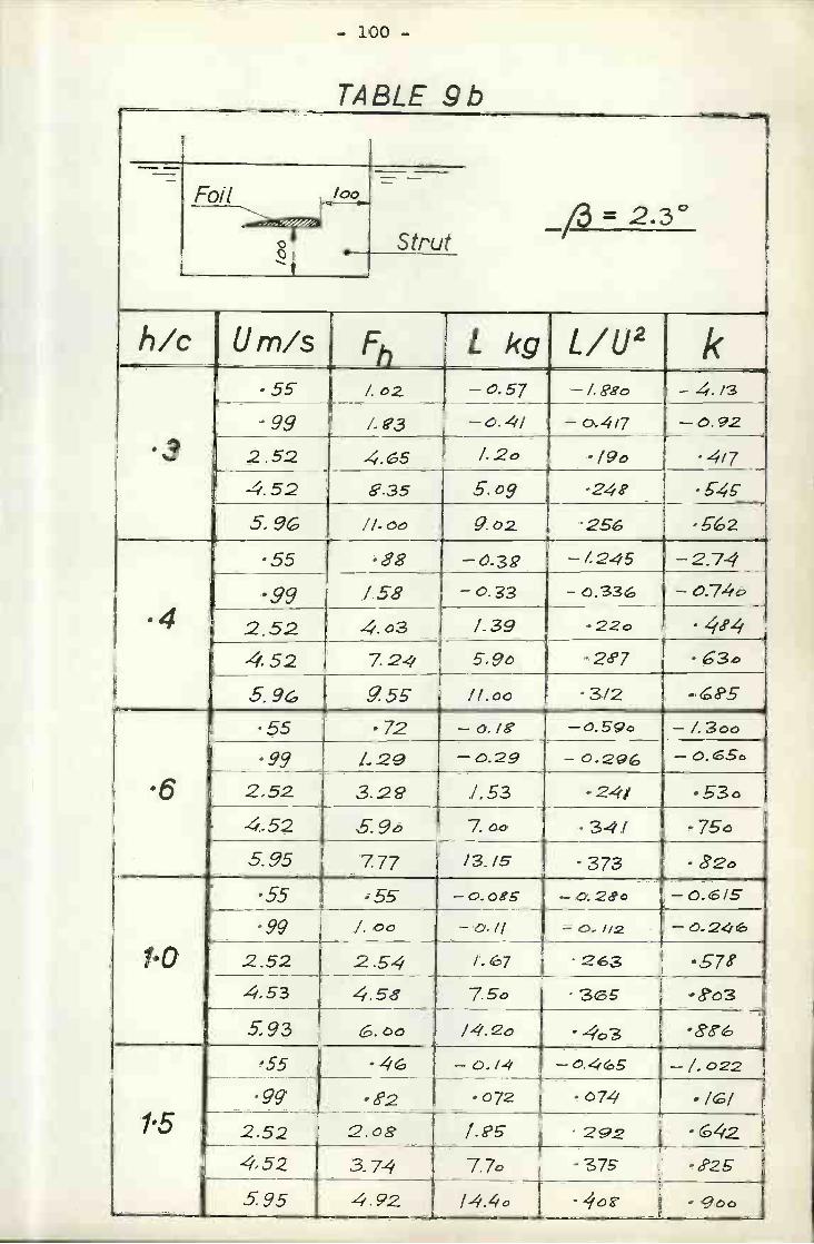
- loo -
TABLE 9b
= 2.3Fo/I loo- -
StrutTh.
h/c U rn/s Fh L kg L / U2 k
.3
-0.57 -/.gg0 -4.13.99 /.3 -0.4/ -0.4/7 -0.92
2.52 45 /.2c 19ö 4í74.52 p.35 5.o9 '248
5.9 /i.c 902 '256
'4
55 8g -O.3g -f245 -2.7.4
.99 /58 -°.3 -&336
2.52 4.03 ¡.39 22c4.52 7.24' 5.9c 2c759c. p55' /f.00 -3/2.55 72 -ó.ig -0.590 _/399___ ¿2g -0.29 - 0.2Q, -
252 3.29 ¡.53 24/ 53ö4.52 5.9e 7oö .3_4f
5.95 7.77 /3./S -373
110
55 .55W -O.2 -0.6/5.99 f o - 0./f - 0. f12 -
2.52 2.5'4 /.7 '263 .57e?
4.53 4.5c 7.5'c 3g o3
593 .òö /4.2e
1'5
'55 -4, -o.14 -Ö.4S -7.022.072 . 74
2.52 2.02 /.& '292 c424' 52 37.4 7.70 - .
595 4.92 /-4.4o -
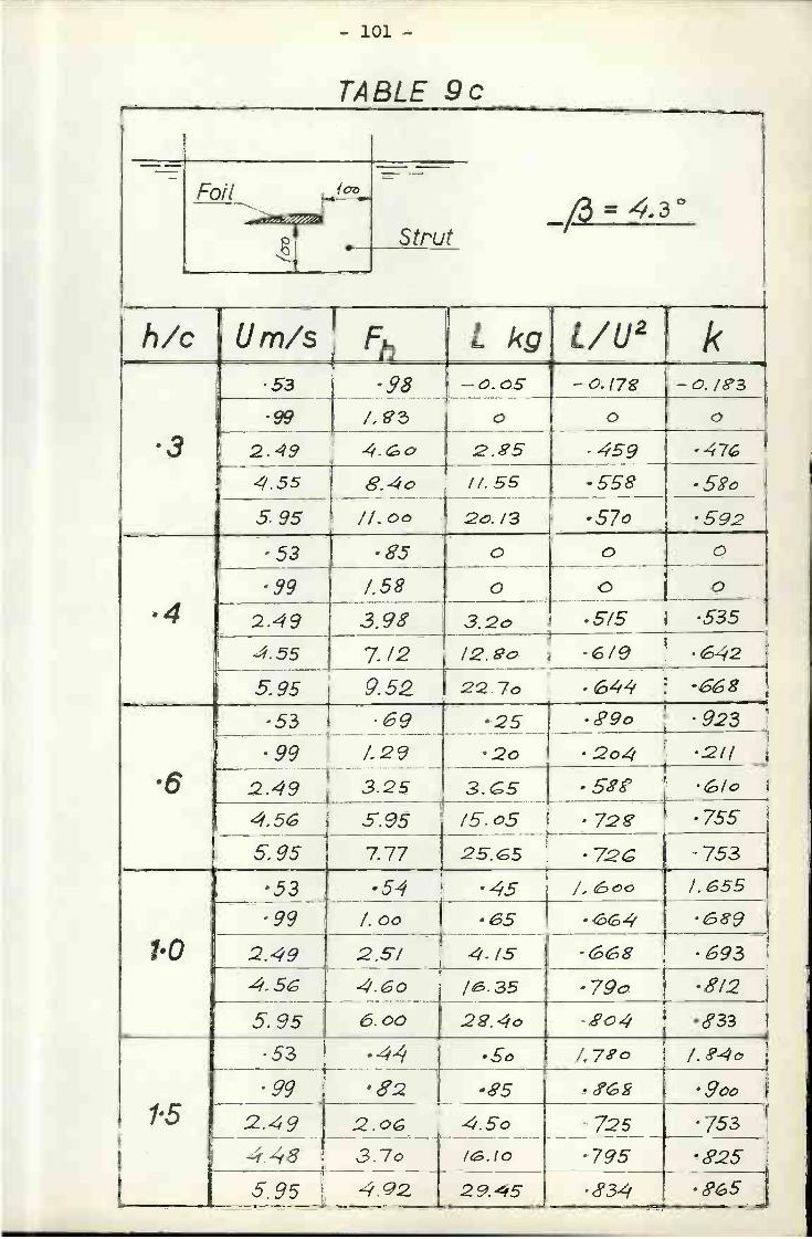
- 101 -
TABLE 9c
¡3 = 4 OFi Ql 1cr
Strut
h/c U rn/s Fh L kg L / U2 k53 98 -0.05 -O.(7' -C./S'3
.99 /.6'3 o O o
2.49 40 2.5 .459 .474.55 8.4o //55 -5-sg
5.95 //.oc 2.13 -57e 592
'4
-53 -cq5 O O
-99 1.58 o o O
2.49 393 3.2c' .5_15 .535
. 55 7. /2 /2. go /9 642595 9.52 227e .644' -66g
6
.53 .9L293.25
25 .890 923F .99 -2e 2o4 211
.2.49 3.5 .5'5.95 /5. c5 - 72g .755
5.95 7.77 25.G5 72G .753
1'O
53 -54 .45 ¿6ccf.cc .5 .4' 689
2.49 2.57 4.15 -66S -6934.5 4.6o
6.00/.35 -79e
5 95 2g,40 . 8c4 833
1'5
.53
'99.4-482
-5e /78o-85 f6 g 9cc
2.49 20G 4.50 725 753
I 448 3.70 /(o -795 825
59 4.g2 29.45 .?3zí
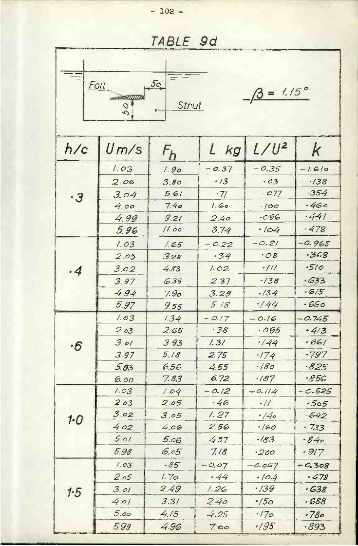
h/c
3
10
15
Urn/s
- 102 -
TABLE 9d
¡3= fJ5Ô
Lkg L/U2-0.37 -0.35
.13 .037/ .077
'34 -081.02 -7/1
2.37 .7353.29 ./34
./441
- o. S255o5
-733
.9/7
/.c3 /.34 -°.'72.O3 2.25 .353.0/ 3.93 ¡.3/3.97 5:/e 2.75 -/74
4.55 /8o.00 783 672 -787
7.03 ¡.04 - o-12 -0.7/42.c3 2.c5 .7/3.02 3.05 ¡.27
254.02 -/05.0/ 5.c 4.57 /83
7/8 2O0598/.ô3 85
2.o5 ¡.70 .7043.oi 2.49 /.2 139.4.0/ 3.3/ 24ô -/505.ôo 4/5 .25 -170
4.%
¡.03 7.90Q.06 3.8o3.o4 5.r/4.co 7.4o
499 9.2/ 2.4°59 3.74 -/04/.O3 /.5 -0.22 -0,272.05 32g3.o23.974.94 7905.97
.700-ö9&
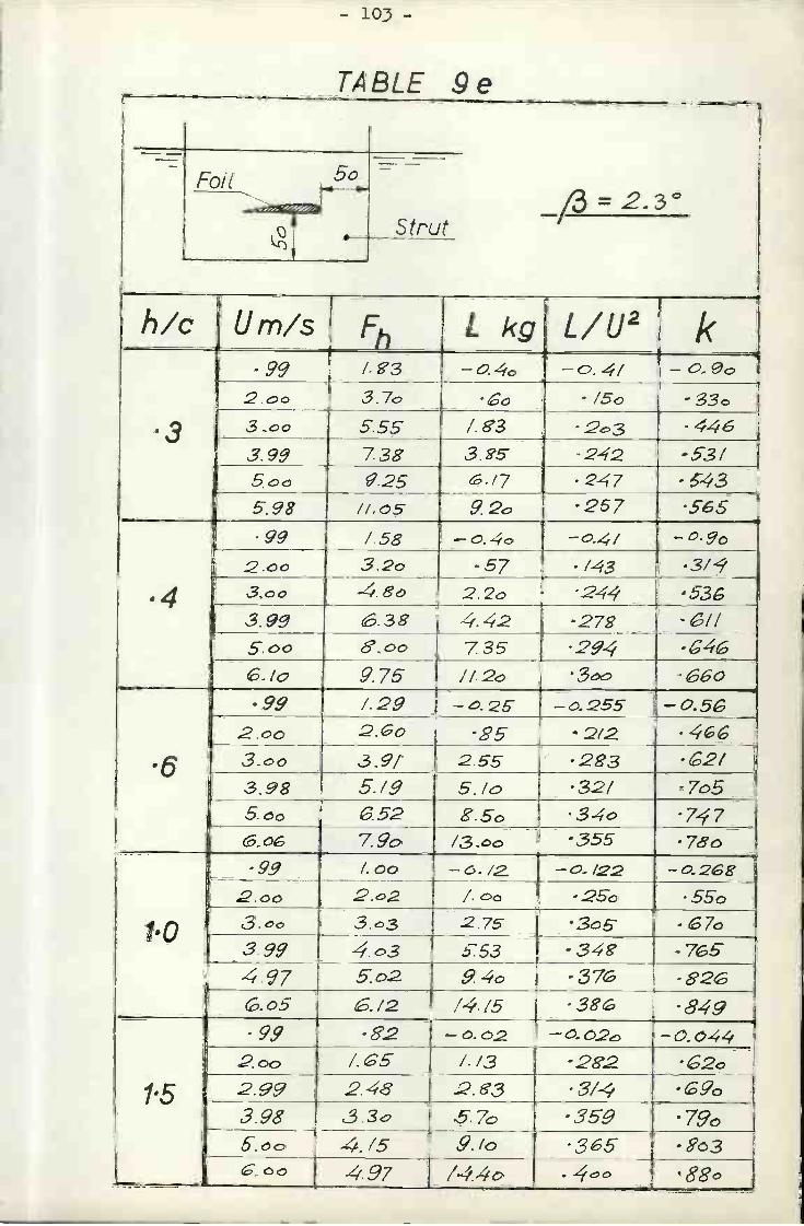
- 103 -
TABLE .9e
¡3 = 2. 3Foil
ru
h/c tim/s Lkg L/U2 k
.3
.99 /.'3 -c24 -0.4/ -O-So2.00 3.70 cGo "/50 "'33o3co 5.55 ¡.83 -23 446399 733 3g5 242 -53/
9.25 ./7 -2-47598 ¡/05 92 257
4
.99 ¡.58 -0.4ó -0.4/2.co 3.2o -57 -/433,00 4.8o 2.2c 2-44 533gg .3S 2 -27g -cG!!5.co 8.00 735 -294
975 //.2 '3oö -G60.99 /29 -'.25 -c.255 -O.5G
2.00 2Go -85 '2/23.00 3.9/ 2.'5 -283398 5./.9 s.i -32f -705500 G52 8.5e '3-4c .77
/3.öô -355 780
10
-2.9 ¡.00 -O./2 -0.122 -0.282.'2 /.o 25o -550
3.o 3.3 2.75 .305_3.99 4. c3 .53 34 - 7654.97 5o2 .4o .37 -82G6 o5 6/2 /4.75 38 849
15
99 -82 -0.02 0. O2 - O. 04/. cG5 ¡.13 282
2.99 2.48 2. e3 - 3/-g3.98 .3o 5.7e 35:9 7906. co 4.75 9. fo 365 - 8ó 3
4.97 /4o ..4cc

O D
ista
nce
from
foil
to le
adin
g ed
ge
valu
esva
lues
of s
trut
50 m
m
- lo
o -e
'-
for
incr
ease
d su
bmer
genc
e du
e
¡'3 =
115
O+
--
-e-
= M
ean
abs
e've
d
The
oret
ical
-er-
corr
ecte
dto
wav
e fo
rmat
ion
- =
____
___
__-n
-h/
c=
15)
¡Ç
'1
6
4
41
AI!É
IÜJ'
hip
uo
:89
i15
23
46
78
910
U
15
gh
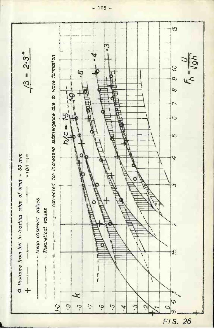
O D
ista
nce
from -ii
-M
ean
foil
The
oret
ical
to le
adin
g ed
ge
valu
es
of s
trut
50 m
m=
loo
--
for
incr
ease
d su
bmer
genc
e ot
ieto
f3 =
23
O+
-II-
--ob
serv
ed-- valu
es ,-co
rrec
ted
wav
e fo
rmat
ion
--
- -
- -
--
- -
.9 6 .5
I
____
__'e
ii
i;i
-- £!i
-
- -
iílIli
P"
3
IIIO
IIL
Wi
.1iiI
I"
4 o4i-
56
7:8
9
f
153
89
10U
15
'J.g
h
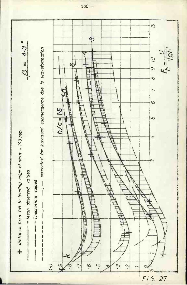
+ D
/sta
ncfr
om = M
eanfo
il
/1
The
oret
ical
to obse
rved
lead
ing
edge
of
valu
es
valu
es
corr
ecte
dstru
tlo
o m
m
for
incr
ease
d su
bmer
genc
e du
e to
43__
___
'I wav
efor
m a
t/on
____
_ __
___
--
- -
10
h/c
1.5
1
Ic_1
.II
6111
1iii
IilIii
iÌ11
1i
1iiï
iii pp
e
r"
45
67
:°J
hV
gh'

3 cm
2
2
cm
- 107 -
U= 2.5 rn/sec
U 6m/sec
= 1.15°
1-15 °
FIG. 28

lo g
The
oret
ical
kva
1ues
cor
rect
ed fo
r in
crea
sed
subm
erge
nce
due
to o
bser
ved
wav
efo
rmat
ion
abov
e hy
drof
oil
h=
dist
ance
from
foil
to u
ndis
tur'b
edw
ater
sur
face
t/c01
1
A=
11o,
=
8910
15
FU
h

- 109 -
FIG. 30
4
.4
Th eor etica I CX h/c -values corrected for ¡n cre se dsubmergence due to observed waveformation above hydrofoil
h = distance from foil to undisturbedwater surface
________
rlI //i
/
IA
.3CLXIVc
rA 44.A, /r /
-A h/c.4.1
h/c = .3
- -
.ddllIlÒ2 03 04 05 06 07 08 09
/3

- 110 -
CASE i U=6m/sec. h/00.04 /3=Q.Q75
L- _-;____-
Observed Streamlines
Theoretical -'j rtex,gmvity termsVr t ex, dipole gravi ty term s
CASE 2 U= 1 897m/sec. ?/c = 004 = 0075
FIG. 31
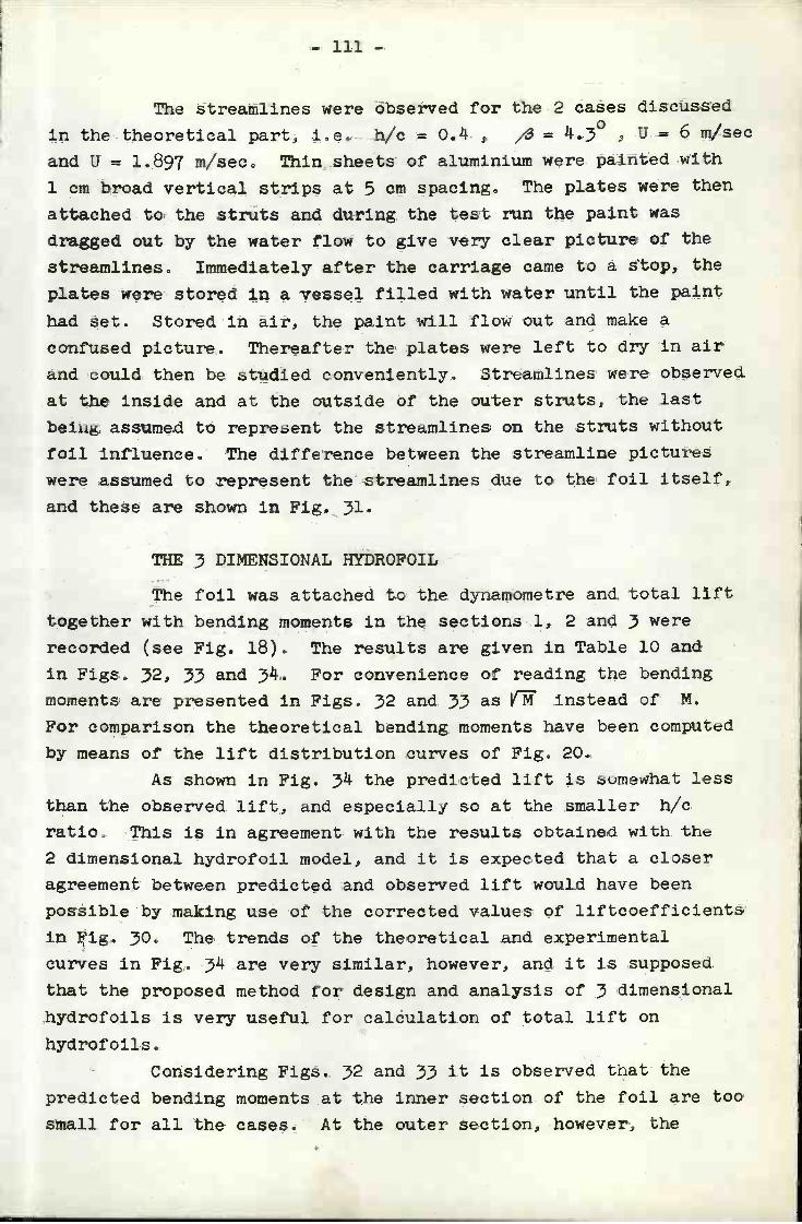
The streamlines were observed for the 2 cases discussed
in the theoretical part, i.e. h/c = , ,,3 = 4.3° , u = 6 rn/sec
and U = 1.897 rn/sec. Thin sheets of aluminium were painted with
1 cm broad vertical strips at 5 cm spacing, The plates were then
attached to the strúts and during the test run the paint was
dragged out by the water flow to give very clear picture of the
streamlines0 Immediately after the carriage came to a stop, the
plates were stored in a vessel filled with water until the paint
had set. Stored in air, the paint will flow out and make a
confused picture. Thereafter the plates were left to dry in air
and could then be studied conveniently. Streamlines were observed
at the Inside and at the outside of the outer struts, the last
being assumed to represent the streamlines on the struts without
foil influence. The difference between the streamline pictures
were assumed to represent the streamlines due to the foil itself,
and these are shown In Fig. 31.
TRE 3 DIMENSIONAL HYDROFOIL
The foil was attached to the dynamometre and total lift
together with bending moments in the sections 1, 2 and 3 were
recorded (see Fig. 18). The results are given in Table 10 and
in Figs. 32, 33 and 34. For convenience of reading the bending
moments are presented in Figs. 32 and 33 as YM instead of M.
For comparison the theoretical bending moments have been computed
by means of the lift distribution curves of FIg. 20.
As shown in Fig. 34 the predicted lift is somewhat less
than the observed lift, and especially so at the smaller h/c
ratio. This is in agreement with the results obtained with the
2 dimensional hydrofoil model, and it is expected that a closer
agreement between predicted and observed lift would have been
possible by making use of the corrected values of llftcoefficients
in Fig. 30. The trends of the theoretical and experimental
curves in Fig. 34 are very similar, however, and it is supposed
that the proposed method for design and analysis of 3 dimensional
hydrofoils is very useful for calculation of total lift on
hydrofoils.
- Considering Figs. 32 and 33 it is observed that the
predicted bending moments at the inner section of the foil are too
small for all the cases. At the outer section, however, the
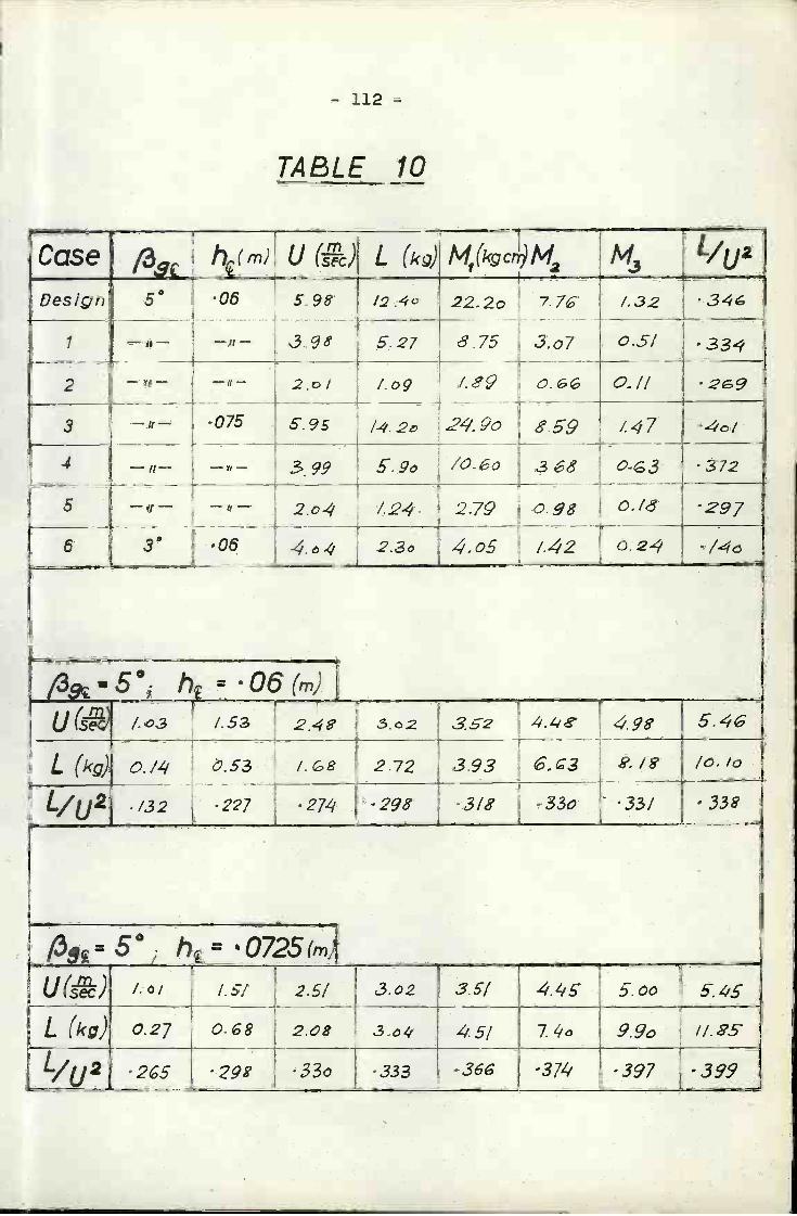
Case
50
¡ih(m) ti (sec
TABLE 10
95'
- 112 -
'4° 22.2o 7.76 1.32 .34'Design 06 5. /2
- Il - 3»8 5.27 8,75 3.07 0.5/ .334- ¡I -i
- (f - 2.o/ 1.09 ¡.89 ô.G 0.1/ 2692 - -3 - ¡I - 075 5.95 /4. 2 24'. 90 8.59 147 40 /
- I, - 3.99 5.9e /O.6o 38 0.3 372-4 - II -
2.79 0.3 0.18 2975 - Il - -(I - 2.o4 ¡.24.
06 4.o4 2.3ö 4,05 ¡.42 /4o6 30
= 0725 (m
I I 1_ ¡.0/ /.51 2.5/ 3.o2 3.5/ 5.00 5.115c, isec
L (kg) 0.27 O.8 2.08 3.04' 45/ 7.4'ö //.5'5
L/U2 25 298 330 .333 36 .374, .397 .39
06(m)1I ¡ f_W.')U tseC.' ¡.03 .53 2.4k' 3.02 3,52 4.98
/0. /0L (kg) 0.53 '. 2.72 3.93
.338227 .274 -298 -3/8 -33ô .33/L/U2 .132
L (kg) (kc M2
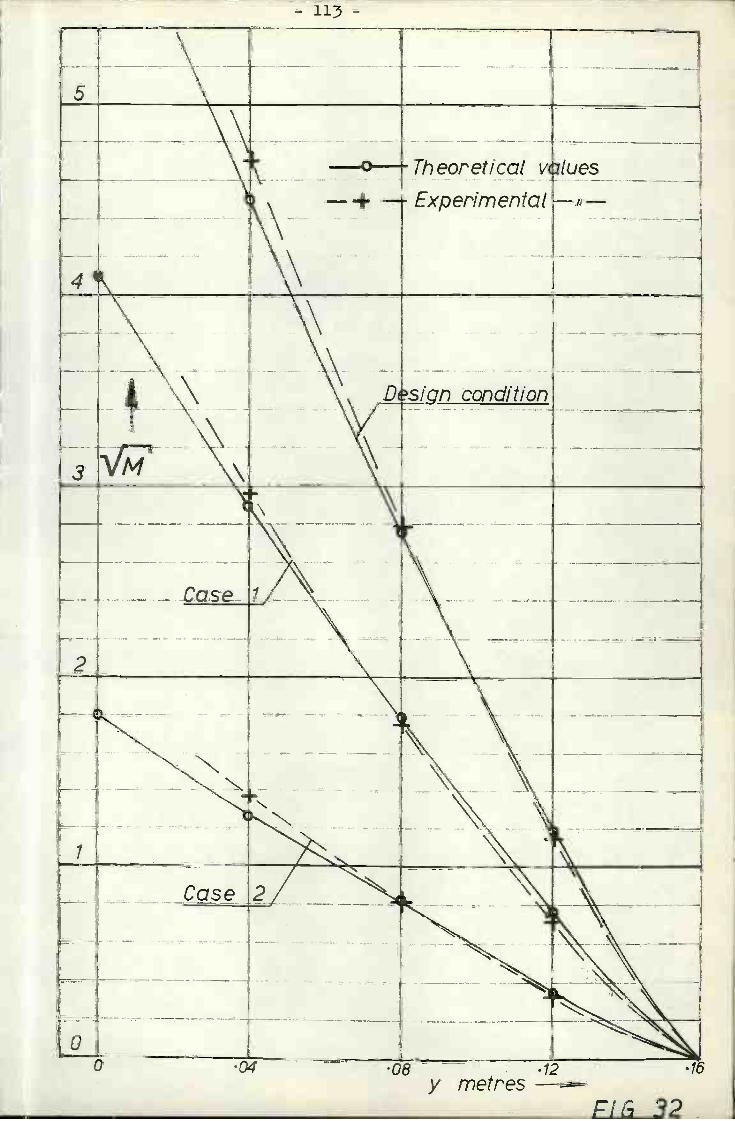
- 113 -
04
- - Theoretical vluesExperimental+- 'i-
Dsign condition\
2
.Case..1
-
- NN
F
i_I
Case 2 1J
o8 .12 16y metres
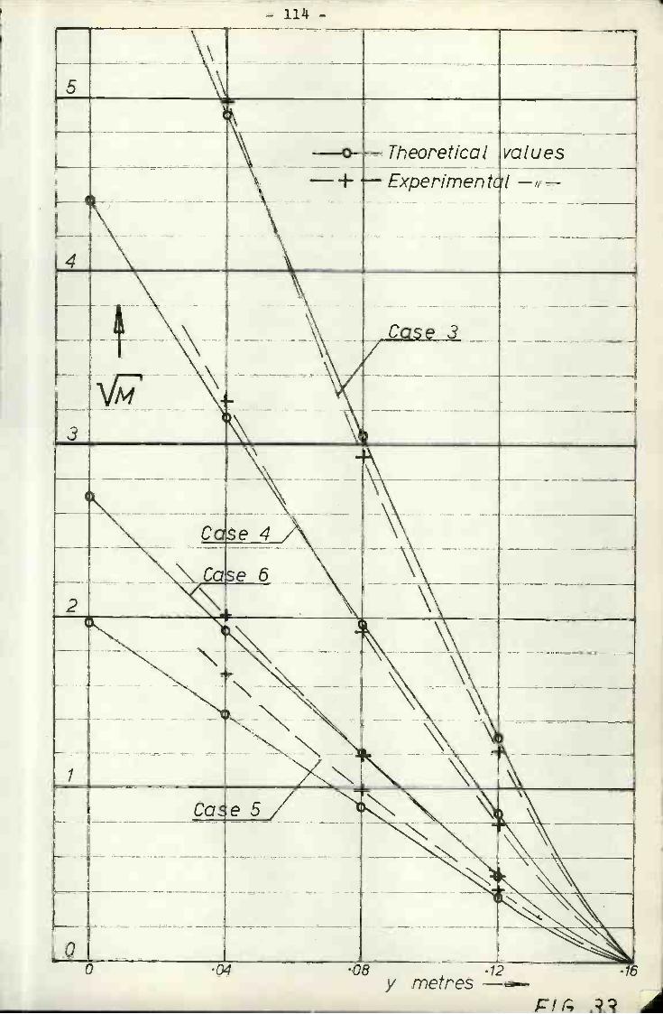
04 08 .12 16y meesc/I; A
\5
'p
- values-o- i
4
- + - 1 ii -
I
-C.
\Ca-.2
o
-
NN
o
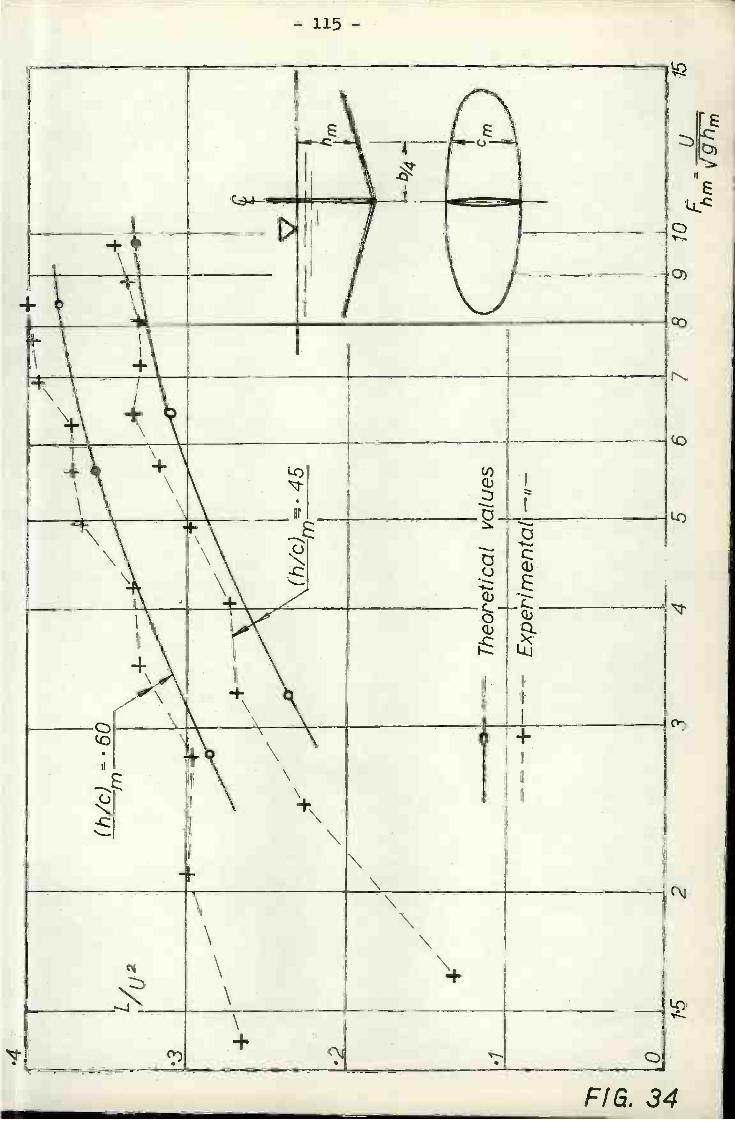
Lu2/
(h/c
= 6
0
i
// uI-/
1(I
//CI
s
- -.
z-,-
\
;
'2
-
-I-"//
//
The
oret
ical
val
ues
---+
----
Exp
erim
enta
l»--
-
152
45
68
915
hrn
gh
predicted moments are too large, except for the cases 5 and 6.The conclusion is that the lift is somewhat overestimated at the
tip of the foil, and somewhat underestimated for the rest of the
toll. The lift discrepancy at the wing tip Is supposed to be a
result of the edge effect described by Jones E22]. Considering
for example that the maximum (or "edge") velocity around an
infinite circular cylinder is 2U while that around a sphere is
1.59 U, it is realized that the edge velocity on the wing is
somewhat less than predicted by theory. Consequently the lift,
which is a function of U2 , is also somewhat less than predicted.
However, the observed bending moment distributions are in
satisfactory agreement with the predicted values, and the proposed
method for design and analysis therefore seems to be useful for
prediction of total lift as well as lift distribution.
DISCUSSI ON
It was shown In the theoretical part that substituting
the hydrofoil by a vortex and a dipole seems to have the following
advantages compared with the substitution by a vortex:
The position of the substitutional vortex and dipole
is fixed to the centre of the hydrofoil.
The complex velocity potential has a forni which is
easier to handle.
The position of the virtual centroid of circulation
seems to agree better with the exact position of this
centroid.
Point 3 may be verified by calculations and experiments, and the
streamline tests described earlier seem to agree with the
theoretical results. These tests indicate for the particular
toil and conditions that there is little to choose between the
systems at high speed, but that the vortex-dipole substitution
is much to be preferred at lower speeds. This result could have
been anticipated from Table 1. It does not seem to be possible,
however, to predict the wave forni and wave height with any
accuracy by substituting the hydrofoil with the vortex-dipole
- 117 -
system, at least not when the submergence/chord ratio is as low
as Q,1. In calculating the circulation reduction factor, on the
other hand, the distance between the hydrofoil and its image is
twice the distance to the water surface, and that makes the
prediction of the relevant perturbation velocities at the stagnation
point of the Joukowski circle much more accurate. There is still
a rather large difference between predicted and observed
circulation at small submergence/chord ratios and especially at
a small angle of attack, Some of the reasons for this discrep-
ancies are:
The wave formation alters the submergence.
The approximate complex velocity potential is less
accurate at small submergence.
)) The method of complying with the Kutta condition is
less satisfactory at small submergences.
The complex velocity potential of the vortex-dipole system was
found by an analytic continuation into the upper region by
applying Schwarz reflection principle. The free surface was then
taken to be y = O , where the complex potential has only real
values, expressed by the stream function y = O. When a wave is
formed above the hydrofoil, there is a better correspondance with
mathematical theory by shifting the position of the real axis to
the wave surface, so that the hydrofoil submergence is increased.
It is shown in the experimental part that this correction greatly
improves the correspondance between theory and experiments at
lower submergence/chord ratios.
Substituting a hydrofoil by a vortex and a dipole at
the foil centre, the following terms of the complex velocity
potential were neglected:
2412')z
z - (' ') 2/ (21e )2
2
The complete potential should have been:
a
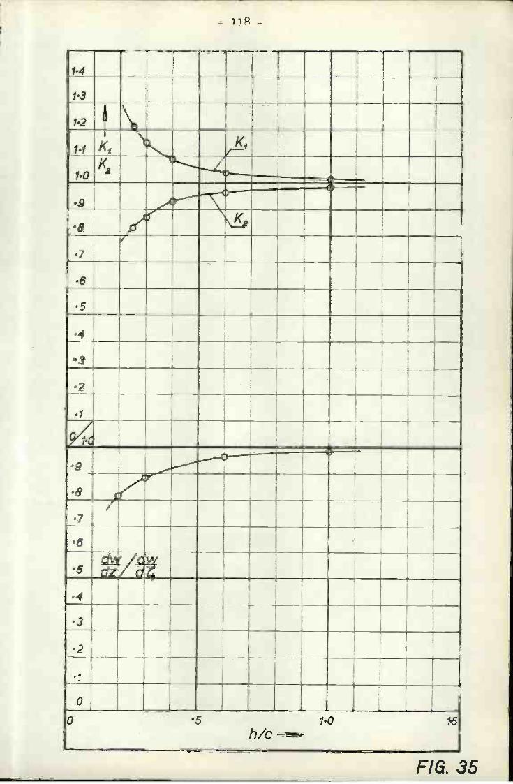
FIG. 35
14
KI
Q
H
'5 Lw /awddz/
.4
.3
2
.4
o
o .5 1.0
h/c
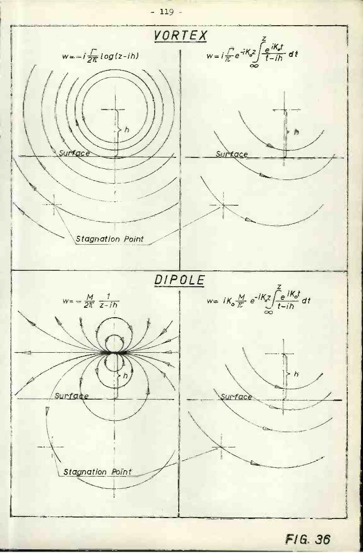
w= _iÇ. log(z-ih)
\stagn at/on
Stagnation ioin t
- 119
FIG. 36
Ml w= iK0-t- e1[e dtW_27r z-Th t-1h
VORTEX z
w= iÇeo2f dt
zDIPOLE

- 120 -
r ¿,,t'a2_2 /20C'C ik'IXACT
/ Ue r-
(2Ze")2.4
J/#;//_(z .1 ¿1-
2 2 f/t (2?)z'j
At h/c = 0.3 and putting z = i 2.k i e10C , which is then
approximately the distance between the foil and its image, we
find:
W = ¿Jz/'-Ç=1og(i75Z)#ô.B7Ua2e0)
£X.4CT 2ii Z
whereas substitution with a vortex and a dipole gives:
1í(a2Ze 0C)
z
Writing the exact complex velocity potential
/aé2e0C)W ¿"z # ¡Ç/og (lc'1z) #LX 4(7
we may compute the values of K1 and K2 corresponding to
different submergence/chord ratios and valid for z = ± i 2h. The
result is given at the top of Fig. 35. Considering now the image
terms of the complex velocity potential of a submerged vortex and
dipole at the point -1h
z
E dist' -il:
z
t' e' «Me -iÇz Ç e a? ,z-Th
*/(\ t-;í
J
rrr
00
'Eô4.

121 -
we may draw the streamlines of this image system as indicated in
Fig. 36. We note that the two terms of the vortex image system
induce velocities at the stagnation point of the Joukowski circle
which are oppositely directed. By computing these velocities for
different conditions, it will be observed that the negatively
rotating image vortex predominates at larger K0 values, whereas
the gravity dependent term predominates at lower K0 values. At
K0 = O this latter term is twice the vortex term, so that the
total image system consists of a simple biplane image vortex.
Considering further the streamlines due to the dipole image system,
and the K1 and K2 values given in Fig. 35, we may draw the
following conclusions:
At high speed the induced velocities from the vortex
and dipole images have the same direction at the stagnation point.
Those predicted from the vortex images are too small and those
predicted from the dipole images are too large, hence the net
result should be satisfactory down to relatively small submergence/
chord ratios.
At low speed the induced velocities from the vortex
and dipole images are oppositely directed at the stagnation point,
and since the predicted velocities due to the vortex system are
too small and those due to the dipole system are too large, we may
conclude that the predicted downwash velocity at the stagnation
point is too large. Hence the predicted circulation is too small.
The above conclusions have been verified by the experiments, and
it is expected that the vortex-dipole substitution should be
satisfactory accurate down to a submergence/chord ratio of say O.,
provided that the increased submergence due to wave formation is
corrected for.
Under point 3) above is mentioned that the method of
complying with the Kutta condition is less satisfactory at small
submergence/chord ratios. It was stated in the theoretical part
that the circulation was evaluated by placing the Joukowskl circle
in the "undisturbed" flow consisting of the free stream together
with the disturbances due to the images. The circulation was
found by making the point -1 eboc on the Joukowski circle a
stagnation point. There are two approximations in this procedure;
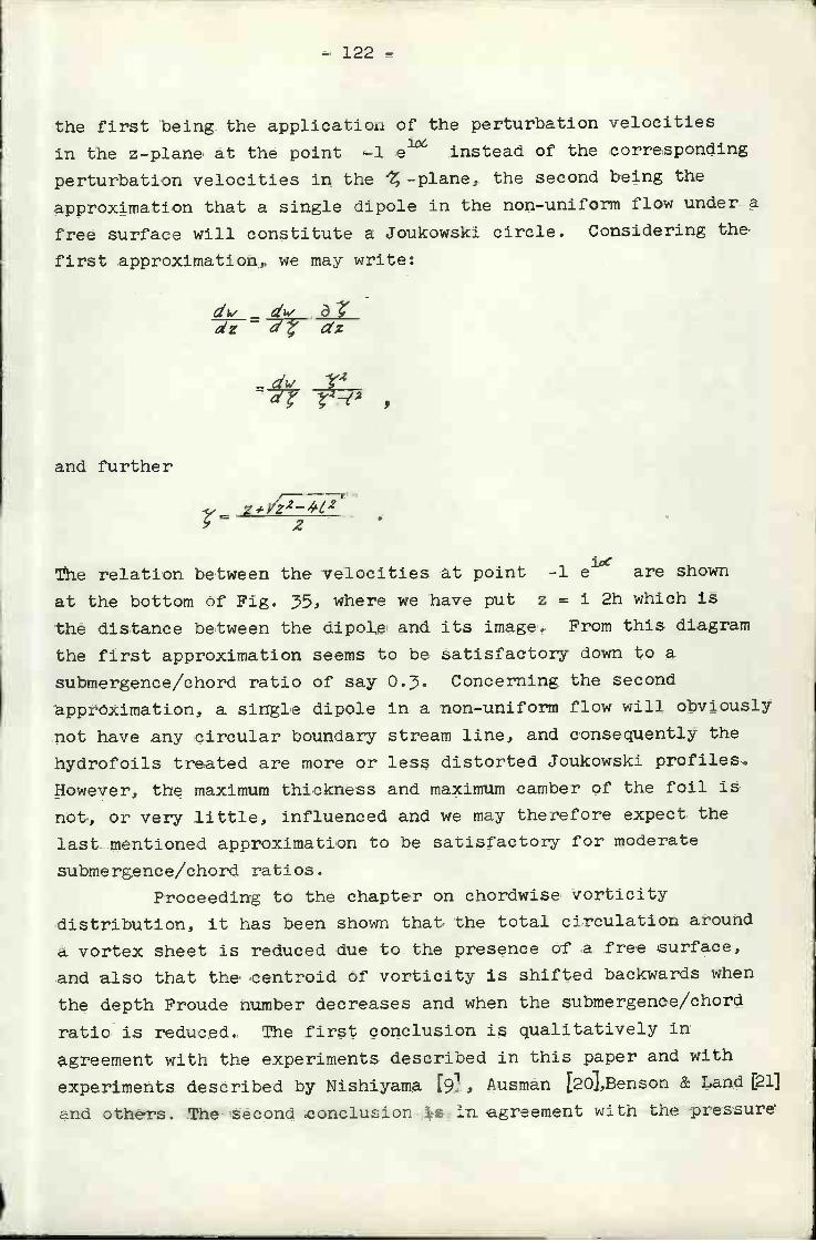
- 122 -
the first being the application of the perturbation velocities
in the z-plane at the point -1 e1° instead of the corresponding
perturbation velocities in the Z -plane, the second being the
approximation that a single dipole in the non-uniform flow under a
free surface will constitute a Joukowski circle. Considering the
first approximation, we may write:
a/k, dv ¿3'dzd a'z
d7 'pand further
.,=2
The relation between the velocities at point -1 e10( are shown
at the bottom of Fig. 35, where we have put z = i 2h which i-s
the distance between the dipole and its image. From this diagram
the first approximation seems to be satisfactory down to a
submergence/chord ratio of say 0.3. Concerning the second
approximation, a single dipole in a non-uniform flow will obviously
not have any circular boundary stream line, and consequently the
hydrofoils treated are more or less distorted Joukowski profiles.
However, the maximum thickness and maximum camber of the foil is
not, or very little, influenced and we may therefore expect the
last mentioned approximation to be satisfactory for moderate
submergence/chord ratios.
Proceeding to the chapter on chordwise vorticity
distribution, it has been shown that the total circulation around
a vortex sheet is reduced due to the presence of a free surface,
and also that the centroid of vorticity is shifted backwards when
the depth Froude number decreases and when the submergence/chord
ratio is reduced. The first conclusion is qualitatively in
agreement with the experiments described in this paper and with
experiments described by Nishiyama [9], Ausman L2olBenson & Land [211
and others. The second conclusion is in agreement with the pressure
s
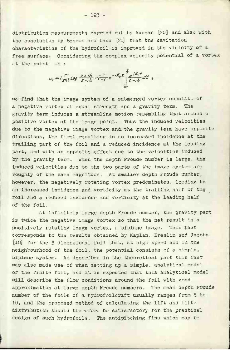
- 123 -
distribution measurements carried out by Ausman 2o] and also with
the conclusion by Benson and Land [21] that the cavitation
characteristics of the hydrofoil is improved in the vicinity of a
free surface Considering the complex velocity potential of a vortex
at the point -h
z
e ¡X(_//
j.t-iíz
we find that the image system of a submerged vortex consists of
a negative vortex of equal strength and a gravity termo The
gravity terrri induces a streamline motion resembling that around a
positive vortex at the image pointu Thus the induced velocities
due to the negative image vortex and the gravity term have opposite
directions, the first resulting in an increased incidence at the
trailing part of the fon. and a reduced incidence at the leading
part, and with an opposite effect due to the velocities induced
by the gravity term. When the depth Froude number is large, the
induced velocities due to the two parts of the image system are
roughly of the same magnitude. At smaller depth Froude number,
however, the negatively rotating vortex predominates, leading to
an increased incidence and vorticity at the trailing half of the
foil and a reduced incidence and vorticity at the leading half
of the foil
At infinitely large depth Freude number, the gravity part
is twice the negative image vortex so that the net result is a
positively rotating image vortex, a biplane image This fact
corresponds to the results obtained by Kaplan, Breslin and Jacobs
[ioj for the 3 dimensional foil that, at high speed and in the
neighbourhood of the foil, the potential consists of a simple,
biplane system. As described in the theoretical part this fact
was also made use of when setting up a simple, analytical model
of the finite foil, and it is expected that this analytical model
will describe the flow conditions around the foil with good
approximation at large depth Froude numbers. The mean depth Freude
number of the foils of a hydrofoilcraf t usually ranges from 5 tolO, and the proposed method of calculating the lift and 11f t-
distribution should therefore be satisfactory for the practical
design of such hydrofoils. The antipitching fins which may be

- 124 -
mounted at the bow of displacement vessels, usually operates at
lower depth Froude numbers, but the submergence/chord ratios are,
on the other hand, relatively large, so that it is expected that
the lift and liftdistribution may be evaluated with good
approximation by means of the proposed method.
RES TiME
The influence on the circulation around a 2 dimensional
hydrofoil due to the presence of a free water surface has been
estimated by substituting the hydrofoil with a suitable vortex
and dipole at the centre of the foil. The influence on the
circulation is presented in the form of a circulation reduction
factor, and it is shown that this factor is a function of speed,
submergence, incidence and foil thickness Some values of the
circulation reduction factor have been computed.
it is further shown that substitution of the hydrofoil
by a vortex at the quarter point of the foil is by no means
adequate. Apart from being dependent on foil geometry and
incidence, the position of the substitution vortex also depends
upon the observation point,
The streamlines around a hydrofoil have been determined
theoretically for two cases by substituting the hydrofoil with a
dipole and a vortex at the centre of the hydrofoil, alternatively
by substitution with a vortex at the centroid of circulation.
The theoretically predicted streamlines have been compared with
the streamlines obtained by experiments, and it is shown that
the two ways of substituting the hydrofoil seem to give the same
degree of approximation to the real flow at high speed. At low
speed, however, the substitution by a vortex and a dipole at the
centre of the hydrofoil seems to give a much better approximation
than substitution with a vortex
The predicted circulation reduction factors have been
compared with reduction factors obtained by experiments and it is
shown that the agreement between theoretical and experimental
reduction factors is satisfactory for moderate submergence/chord
ratios. When the theoretical values of the circulation reduction
factors are corrected for increased submergence due to the

125 -
observed wave formation above the hydrofoil, there is an improved
agreement between predicted and observed circulation reduction at
all submergence/chord ratios and depth Froude numbers.
The chordwise distribution of vorticity has been determined
by substituting the hydrofoil with a vortex distribution along the
mean line together with the images of these vortices. Some values
of coefficients determining the vortex distribution bave been
obtained by means of an electronic computer. From these
coefficients the vortex distribution and total lift have been
evaluated.
A semi 3 dimensional method has been suggested for the
calculation of lift on submerged, finite span hydrofoils. A hydro-
foil has been designed by means of this method, and for the same
hydrofoil the total lift as well as the spanwise liftdistribution
have been found for different off design conditions. A series of
experiments were performed and the observed total lift values as
well as the lift distribution compared satisfactorily with the
predicted values. It is expected that the proposed method for
calculation of total lift and liftdistribution on finite hydrofoils
with sweep back and dihedral, is convenient in use and sufficiently
accurate for engineering purposes.
Description and drawings are given for a 6 component
dynamometre which was designed for the main purpose of testing
hydrofoil models.

[2] Strandhagen, A.G.
and Seikel, G.R.
[4] Jeffreys, H. and
Jeffreys, BS0
[51 Bleick, W.E.:
[7) Lunde, J0K:
- 126 -
"On the Wave-Making Resistance and Lift
of Bodies Submerged in Water."
Transaction of the Conference on the
Theory of Wave Resistance, USSR, Moscow
1937. Technical and Research Bulletin
No. i-8, Society of Naval Architects and
Marine Engineers, 1951.
"Lift and Wave Drag of Hydrofoils".
Transaction of the Fifth Midwestern
Conference on Fluid Mechanics,
pp. 351-364, 1957.
[31 Mime-Thomson, L.M.: "Theoretical Aerodynamics"
MacMillan and Co,, Ltd., London 1948.
"Methods of Mathematical Physics",
University Press, Cambridge 1950.
"Tables of Associated Sine and Cosine
Integral Functions and of Related
Complex-Valued Functions"
Technical Reports No0 10, United States
Naval Postgraduate School, Monterey,
California, 1953,
"On the Linearized Theory of Wave
Resistance for Displacement Ships in Steady
and Accelerated Motion".
Transaction Society of Naval Architects
and Marine Engineers 1951, pp. 24-76.
[6] "Tables of Sine, Cosine and Exponential
Integrals, VoL I".
Federal Works Agency, Work Project
Administration for the City of New York,
19240.
REFERENC ES
[i] Kotchin, N.E.:
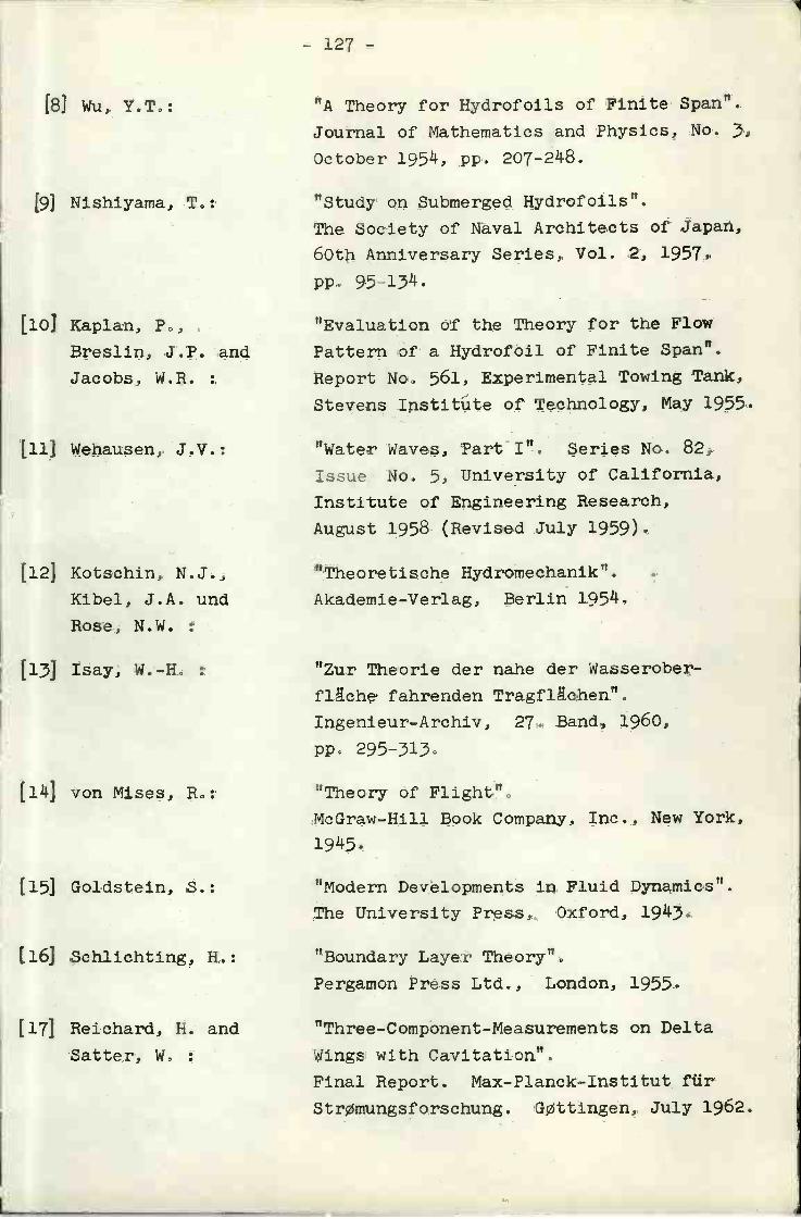
[8] Wu, Y.T,:
[9) Nishlyama, T0:
[loi Kaplan, P,
Breslin, J.P. and
Jacobs, W.R.
Iii] Wehausen, J.V.:
[121 Kotschin, N.J.,
Kibel, J.A. und
Rose, N.W.
[i3J Isay, W.-H,
{ i4] von Mises, R.:
(151 Goldstein, S.:
[16] Schlichting, H.:
[171 Reichard, H. and
Satter, W
- 127 -
"A Theory for Hydrofoils of Finite Span".
Journal of Mathematics and Physics, No0 3,October 1954, pp. 207-248.
"Study on Submerged Hydrofoils".
The Society of Naval Architects of Japan,
60th Anniversary Series, Vol. 2, 1957,pp. 95-134.
"Evaluation of the Theory for the Flow
Pattern of a Hydrofoil of Finite Span".
Report No 561, Experimental Towing Tank,
Stevens Instíti.te of Technology, May 1955.
"Water Waves, PartI". Series No. 82,
Issue No. 5, University of California,
Institute of Engineering Research,
August 1958 (Revised July 1959).
"Theoretische Hydromechanik".
Akademie-Verlag, Berlin l954
"Zur Theorie der nahe der Wasserober-
fl.che fahrenden Tragflachen",
Ingenieur-Archiv, 27. Band, 1960,295313e
"Theory of Flight".
McGraw-Hill Book Company, Inc., New York,
1945.
"Modern Devélopments in Fluid Dynamics".
The University Press, Oxford, 1943.
"Boundary Layer Theory"0
Pergamon Press Ltd., London, 1955.
"Three-Component-Measurements on Delta
Wings with Cavitation".
Final Report. Max-Planck-Institut fiir
StrØmungsforschung. GØttingen, July 1962.
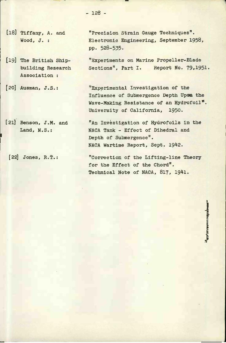
f20] Ausman, J.S.:
[22] Jones, R.T.:
[211 Benson, J.M. and
Land, N.S.:
- 128 -
Tiffany, A. and "Precision Strain Gauge Techniques".
Wood, J. Electronic Engineering, September 1958,pp. 528-535.
The British Ship- "Experiments on Marine Propeller-Blade
building Research Sections", Part L Report No. 79,1951.Association
"Experimental Investigation of the
Influence of Submergence Depth Upon the
Wave-Making Resistance of an Hydrofoil".
University of California, 1950.
"An Investigation of Hydrofoils in the
NACA Tank - Effect of Dihedral and
Depth of Submergence".
NACA Wartime Report, Sept. 1942.
"Correction of the Lifting-line Theory
for the Effect of the Chord".
Technical Note of NACA, 817, 1941.
I