A METHOD FOR QUICK ESTIMATION OF ENGINE MOMENT OF …

Mrdja, P. D., et al.: A Method for Quick Estimation of Engine Moment of Inertia ... THERMAL SCIENCE: Year 2018, Vol. 22, No. 3, pp. 1215-1225 1215

A METHOD FOR QUICK ESTIMATION OF ENGINE MOMENT OF INERTIA BASED ON AN EXPERIMENTAL ANALYSIS OF

TRANSIENT WORKING PROCESS

Predrag D. MRDJA *, Nenad L. MILJI], Slobodan J. POPOVI], and Marko N. KITANOVI]

Faculty of Mechanical Engineering, University of Belgrade, Belgrade, SerbiaOriginal scientific paper

https://doi.org/10.2298/TSCI170915224M

This paper presents an unconventional approach in a fast estimation of the over-all engine inertia based on engine testing under transient condition (acceleration and deceleration) with simultaneous in cylinder working process analysis and fric-tion losses estimation. The presented procedure is based on a single slow dynamic slope full load engine speed sweep test which, coupled with a simple lumped-mass engine dynamometer model, provides correct overall engine inertia estimation. Compared with the more conventional approaches in deriving information on en-gine inertia, besides its speed and accuracy, presented procedure provides more in depth information on both engine’s dynamic response and friction as a surplus. Key words: internal combustion engine transient working process analysis,

engine inertia, dynamic engine testing, engine friction losses

Introduction

A typical automotive powertrain environment exploits the internal combustion (IC) engine in an extremely dynamic manner. Thus, engine processes transient behaviour has been in focus of research and optimization for years. Present and future ultimate goals in IC engine development, related almost exclusively to the fuel economy and exhaust emission improve-ment, can hardly be achieved without intensive dynamic testing of engines. Therefore, a full attention of IC engine researchers is given to the improvement of dynamic testing procedures, transient data analysis and reliable process information deduction. Engine transients can be characterized through single or simultaneous load and speed change of the engine. The lat-ter, involving the engine speed change containing mechanical inertia related effects which, in overall, blurs the picture of the engine’s working process itself. Hence, compensation and elimination of engine inertia issues is of great importance in transient working process analysis, and this can be achieved only by exact identification of engine mechanical inertia parameters.

In the last few years, the development of dynamic engine test procedures is in focus of numerous scientific research institutes, Universities and leading companies in the automotive industry. The main goal of those research endeavours is aimed at maximizing testing automa-tion and therefore at reducing needed testing time and founds resources. During the power-train development process, and especially during engine optimization for emission legislations, in-vehicle tests are the slowing factor [1, 2], and for that reason, most of the tests are transferred to the driving cycle highly dynamic engine test stands [3]. Dynamic engine testing has many * Corresponding author, e-mail: [email protected]

Mrdja, P. D., et al.: A Method for Quick Estimation of Engine Moment of Inertia ... 1216 THERMAL SCIENCE: Year 2018, Vol. 22, No. 3, pp. 1215-1225

advantages and disadvantages compared to the steady-state approach, but for some applica-tions, the dynamic change of the engine operating point is an unavoidable condition. In general, simulation of a driving cycle represents certain changes with respect to engine load and speed over time. Usually, the engine speed is controlled in closed loop operation by the dynamometer control unit using the information of angular speed over the dyno angular speed encoder. On the other hand, engine torque is also controlled in the closed loop, relying on the torque meter (TM) or force transducer readings. At this point care must be taken regarding rotational movement elements and their mass moment of inertia influence [4, 5]. Because of variable engine speed during the driving cycle, the torque-measuring device will be affected by a particular amount of inertia-induced torque. Depending on the test-bed configuration, elements such as the engine, drive shaft and the dynamometer needs to be evaluated in terms of moment of inertia.

Conventional approach in obtaining info on the inertia of engine’s moving parts is relying on previous knowledge and information from the designing stage of the engine itself or on a simple free engine deceleration test where subtle changes in engine friction and real engine working conditions influences are neglected. The motivation, behind the research presented in this paper, is drawn exactly upon the idea to overcome this issue and estimate engine overall moment of inertia in a fast manner but within the real operating conditions and full identifica-tion of the friction losses as well.

In this paper analysis will be conducted on results derived by means of a basic lumped-mass model of a system consisting of an engine’s (and its axillaries) moving elements, drive shaft and dyno coupling, with a focus on TM readings as a source of system behaviour infor-mation.

Two different approaches of estimating the engine moment of inertia will be pre-sented. The first method relies on statistical analysis of estimated inertia values by means of previously obtained steady-state engine experimental results. The second approach is based on iterative prediction of engine moment of inertia combined with minimization of friction loss-es hysteresis within the dynamic excitation. The obtained results are very similar using those

methods, but the second one is recommended because less data is needed.

Experimental installation

For the purpose of this experiment, the PSA DV4TD 8HT (1.4 l, 40 kW, 8 valves, compression ignition, turbocharged, non-in-tercooled version) engine was coupled with an AC dynamometer. Basic engine test-bed com-ponents and some of the measuring points are overviewed briefly in the fig. 2. Beside param-eters available on the engine on-board diag-nostics, the installation was equipped with ad-ditional measuring chains, where the key ones for the experiment are described in the tab. 1.

All time-resolved parameters were ac-quired using a multifunctional National Instru-ments NI PXI-6229 and NI PXI-6123 acqui-sition cards as a part of the NI PXI platform [6]. The engine was equipped with an optical

Table 1. Test-bed key sensor specificationDescription Sensor type

Engine speed Optical encoder, AVL 365C

Engine torque Torque sensor, HBMT40

Cylinder 1-4 pressure indicating

AVL GM12D + Micro IFEM Piezo Amp.

DYNAMOMETERDYNO

control

AVL

IndiMaster

Acquisition

conditioning

device

NI PXI

main

application

AVL

CAMEO

Automation

application

Online data

analysis

TEST CELL CONTROL ROOM

AVL

IndiCom

ENGINE TEST CELL

Additional engine test bed systems

ECU

OBD

ENGINE

Drive shaft TM

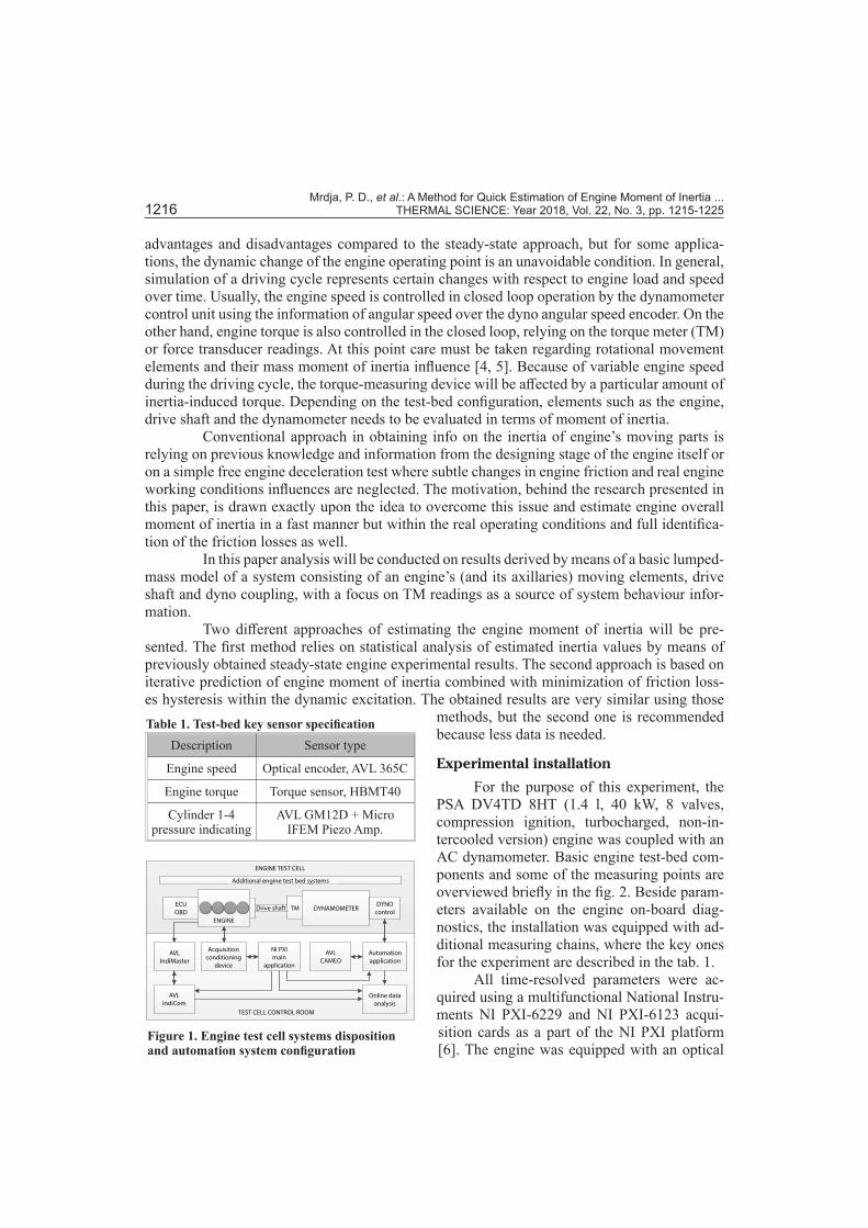
Figure 1. Engine test cell systems disposition and automation system configuration


incremental encoder and with piezoelectric pressure transducers on all four cylinders. Rest of the in-cylinder pressure indication system was completed with AVL charge amplifiers coupled with an embedded hardware platform for engine indicating [7], the AVL IndiModule 621. The AVL IndiCom [8] software solution has been used for engine indicating data visualization, measuring, and data manipulation. For defining the control sequence and setting the dynamic regime, the AVL CAMEO [9] software has been used, while a mediator in Modbus communi-cation between CAMEO and the dynamometer control module has been in-house developed NI LabVIEW [10] application. A test bench schematic, along with the essential data flow between components is shown in the fig. 1.

Test procedure

The conducted experiment was very short, similar to those performed by Godburn et al. [11]. Engine speed was swept in two predefined cycles with gradients of ±5.59 rad /s2 and ±16.06 rad /s2, respectively, with ramp periods of 15 seconds in both cases. The main idea was to vary engine speed over time in a predefined cycle. Precisely, the engine was accelerated with

DA

Q

p IM

T IM

T T1

E-Gas

Torque

Tw

T Oil

pOil

p a

T a

a

T C

tinj

α inj

n

ECU

WG

MFM

n

p inj

EGRV

AT/M

T F

pinj

GA

T MFM

E-Gas

G F

OBD II

μ IFEM p

Ind

imas

ter

Dy

no

Co

ntr

ol

Au

tom

ati

on

Sy

ste

m

Abbrv. Description

MFM Mass air �ow meter-

WG Turbine waste-gate

C Compressor

OBD On-board diagnostic interface

T Turbine

EGRV Exhaust gas recirculation valve

FC Fuel conditioner

FCMS Fuel consumption measurement system

DYNO AC dynamometer

E-Gas Engine torque demand control

OC Oxi-cat

μ IFEM p Amplifer for piezo-electric in-cylinder

pressure transducers

AT/M Atmospheric measurement module

ECU Engine electronic control unit

FCMS

FC

OC

Meas. Description

G F Fuel mass �ow-

G A Air mass l owf

T IM, p IM Inlet manifold temperature & pressure

pinj, α inj Fuel injection pressure & start of injection angle

tinj Fuel injection duration

T T1 Turbine inlet temperature

T Oil, p Oil Oil temperature & pressure

T w Engine coolant temperature

T a, p a, φ a Atmospheric air temperature, pressure and humidity

DYNO

Engine Data

Manufacturer

Model

Type

Bore 73.7 mm

Stroke 84.0 mm

Rated power 40 kW 4000 minat–1

Rated Torque 130 Nm

Fuel injectionsystem

Common rail

Turbocharger KP35 (3K-BW)

Bore 73.7 mm

Stroke 84.0 mm

PSA group

DV4TD 8HT

CI; turbocharged, non-intercooled;

Figure 2. Engine test-bed disposition


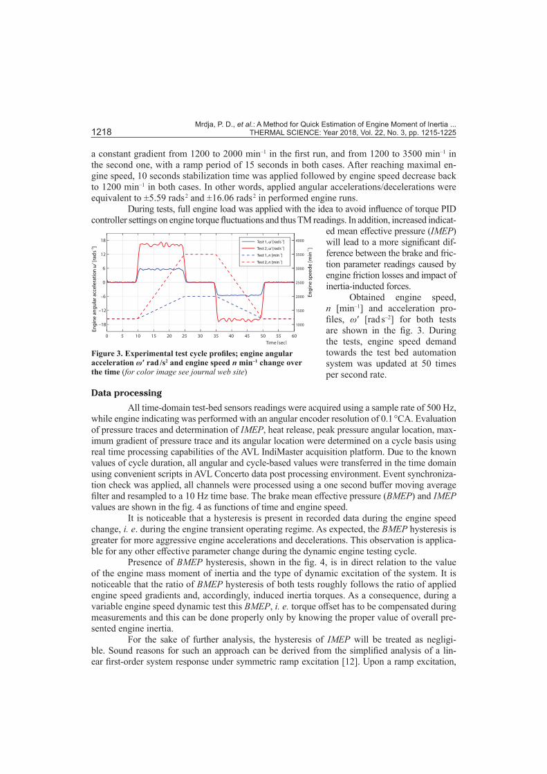
a constant gradient from 1200 to 2000 min–1 in the first run, and from 1200 to 3500 min–1 in the second one, with a ramp period of 15 seconds in both cases. After reaching maximal en-gine speed, 10 seconds stabilization time was applied followed by engine speed decrease back to 1200 min–1 in both cases. In other words, applied angular accelerations/decelerations were equivalent to ±5.59 rads 2 and ±16.06 rads 2 in performed engine runs.

During tests, full engine load was applied with the idea to avoid influence of torque PID controller settings on engine torque fluctuations and thus TM readings. In addition, increased indicat-

ed mean effective pressure (IMEP) will lead to a more significant dif-ference between the brake and fric-tion parameter readings caused by engine friction losses and impact of inertia-inducted forces.

Obtained engine speed, n [min–1] and acceleration pro-files, ωʹ [rad s–2] for both tests are shown in the fig. 3. During the tests, engine speed demand towards the test bed automation system was updated at 50 times per second rate.

Data processing

All time-domain test-bed sensors readings were acquired using a sample rate of 500 Hz, while engine indicating was performed with an angular encoder resolution of 0.1 °CA. Evaluation of pressure traces and determination of IMEP, heat release, peak pressure angular location, max-imum gradient of pressure trace and its angular location were determined on a cycle basis using real time processing capabilities of the AVL IndiMaster acquisition platform. Due to the known values of cycle duration, all angular and cycle-based values were transferred in the time domain using convenient scripts in AVL Concerto data post processing environment. Event synchroniza-tion check was applied, all channels were processed using a one second buffer moving average filter and resampled to a 10 Hz time base. The brake mean effective pressure (BMEP) and IMEP values are shown in the fig. 4 as functions of time and engine speed.

It is noticeable that a hysteresis is present in recorded data during the engine speed change, i. e. during the engine transient operating regime. As expected, the BMEP hysteresis is greater for more aggressive engine accelerations and decelerations. This observation is applica-ble for any other effective parameter change during the dynamic engine testing cycle.

Presence of BMEP hysteresis, shown in the fig. 4, is in direct relation to the value of the engine mass moment of inertia and the type of dynamic excitation of the system. It is noticeable that the ratio of BMEP hysteresis of both tests roughly follows the ratio of applied engine speed gradients and, accordingly, induced inertia torques. As a consequence, during a variable engine speed dynamic test this BMEP, i. e. torque offset has to be compensated during measurements and this can be done properly only by knowing the proper value of overall pre-sented engine inertia.

For the sake of further analysis, the hysteresis of IMEP will be treated as negligi-ble. Sound reasons for such an approach can be derived from the simplified analysis of a lin-ear first-order system response under symmetric ramp excitation [12]. Upon a ramp excitation,

Time [sec]

0 5 10 15 20 25 30 35 40 45 50 55 60

–18

–12

–6

0

6

12

18

1000

1500

2000

2500

3000

3500

4000Test 1, ’ [rads ]ω–2

Test 2, ’ [rads ]ω–2

Test 1, [min ]n–1

Test 2, [min ]n–1

En

gin

e a

ng

ula

r a

cce

lera

tio

n[r

ad

s]

ω’

–2

En

gin

e s

pe

ed

e [

min

]–

1

Figure 3. Experimental test cycle profiles; engine angular acceleration ωʹ rad /s2 and engine speed n min–1 change over the time (for color image see journal web site)


the first-order system response is constantly below the steady-state level line, i. e. an offset response is evident. Changing the excitation ramp sign causes the sign change of the offset response also. If the system time constant is consider-ably slower than excitation ramp time, than the response offset is small enough and can be neglect-ed. Moreover, by applying a sym-metric ramp, with the same but opposite gradients, complete com-pensation of the response offset can be expected. A slow enough excitation ramp is a key element of the slow dynamic slope (SDS) testing methodology which is used for quasi-stationary measurements [13]. Figure 5(a) shows an exam-ple of gathered engine response by applying constant speed torque ramp excitation through the SDS

En

gin

eTo

rqu

e[N

m]

Turb

ine

Inle

tTe

mp

era

ture

[°C

]

IME

P[b

ar]

15

12.5

10

7.5

5

2.5

0

500

450

400

350

300

250

200

150

125

100

75

50

25

0

0 20 40 60 80 100 120 140

Time [s]

Engine torque

Turbine inlet temperature

IMEP

IME

P[b

ar]

15

12.5

10

7.5

5

2.5

0

Turb

ine

Inle

tTe

mp

era

ture

[°C

]

500

450

400

350

300

250

200

0 20 40 60 80 100 120 140

Engine torque [Nm]

Turbine inlet temperature

IMEP

(a) (b)

Figure 5. A dynamic engine testing procedure based on SDS methodology; engine response from symmetric torque ramp sweep in duration of 120 seconds at 2500 min–1

Figure 4. Measured BMEP and IMEP; approach. It can be seen that the (a) change in a time, (b) engine speed domainresponse hysteresis depends on the (for color image see journal web-site)system time constant. Variables heavily influenced by process inertia have much larger hysteresis than fast responding ones. Figure 5 (b) shows how fast the response of IMEP is with a SDS cycle duration of only 120 seconds. This provides a conclusion that even faster ramps could be applied with negligible offset expectation.

Time [sec]

8

9

10

11

12

13

14

Test 1, [bar]BMEP

Test 2, [bar]BMEP

Test 1, [bar]IMEP

Test 2, [bar]IMEP

a)

Engine Speed [min ]–1

1000 1500 2000 2500 3000 35008

9

10

11

12

13

14

0

1

2

3

4

5

6

Test 1, [bar]BMEP

Test 2, [bar]BMEP

Test 1, [bar]IMEP

Test 2, [bar]IMEP

Steady-state FMEP [bar]

b)

BM

EP

[b

ar]

, IM

EP

[b

ar]

Ap

pro

xim

ate

d s

tea

dy

sta

te F

ME

P [

ba

r]

BM

EP

[b

ar]

, IM

EP

[b

ar]

0 5 10 15 20 25 30 35 40 45 50 55 60


Engine torque measurement – theoretical aspects

For further analysis, a simplified lumped-mass model of engine test-bed installation con-sisting of the engine (E), the drive shaft (DS), and the dynamometer (D) is presented in the fig. 6 and described in the tab. 2. Rotational masses oppose angular acceleration, ωʹ, with the momentum caused by the moment of inertia of named elements (JE, JDS, JD) in the opposite direction of angular acceleration. Dynamom-eter and drive shaft suppliers usually provide information about moment of inertia, in partic-ular: JDS = 0.1 kgm2 and JD = 0.65 kgm2.

Table 2. Symbols related to fig. 6Name Description Comment

TEI Indicated engine torque Measured value. Depends on operating point stabilizationTEF Engine friction losses Unknown value for dynamic regimesTDF Dynamometer friction losses Unknown value with negligible impact TDB Dynamometer brake torque Unknown value (possible indirect calculation)

TM Torque meter device Measured value. The difference between generated torque of two machines (engine and the dynamometer)

JE Engine moment of inertia Required value (scalar). Does not depend on operating point stabilization

JDS Drive shaft moment of inertia A known valueJD Dynamometer moment of inertia A known valueωʹ Engine angular acceleration Measured value

The dyno friction losses torque, TDF, is negligible in our case, but generally exists and mainly depends on the angular speed, ω. For the majority of modern engine testing installa-tions, the value of effective dynamometer braking torque, TDB, is internally controlled. The sum of TDF and TDB torque is measured using a shaft-mounted TM or a housing mounted force trans-ducer and it is possible to assign this value to the engine effective torque, but only in steady- -state operating conditions in terms of angular acceleration ωʹ, thus ωʹ = 0 rad / s2.

In the general case, the following equation of the system’s rotational motion and mo-mentum equilibrium could be written: ( )EI EF DB DF E DS D 0T T T T J J J ω′− − − − + + = (1)

The torque values on each side of the TM can be expressed: ( )TM EI EF E DST T T J J ω′= − − + (2)

TM DB DF D DB D DF| 0T T T J T J Tω ω′ ′= + + ≅ + ≅ (3)

There is a certain limit concerning the maximal value of the dynamometer acceler-ation that depends on the maximum AC machine applied torque and its moment of inertia in addition to:

TDB

Dyno

TMDrive shaft

Engine

ω

ω’ > 0ω’ < 0

TEF

TEI

JE · ’ω

JDS · ’ω

TDF

JD · ’ω

Figure 6. Schematic presentation of the simplified lumped-mass model of the engine test-bed system


EI EF ME DS | 0TT T TJ J ω

ω− − ′= − ≠

′ (4)

The unknown variable in the eq. (4), which is needed for the direct calculation of engine moment of inertia, JE, is the value of the engine friction losses torque, TEF, obtained in dynamic conditions as specified by the experiment set-up. Values of indicated engine torque, TEI, and TM readings, TTM, are obtained from IMEP and BMEP sweeps shown in fig. 4.

In order to overcome the lack of information regarding the TEF, the results of steady- -state engine testing were used. The difference between the brake and indicated parameters, which resulted in engine friction losses torque T SS

EF has been approximated using steady-state data.

SS

SS SS SS EI EF MEF EI TM E1 DS | 0TT T TT T T J J ω

ω− − ′= − ⇒ = − ≠

′ (5)

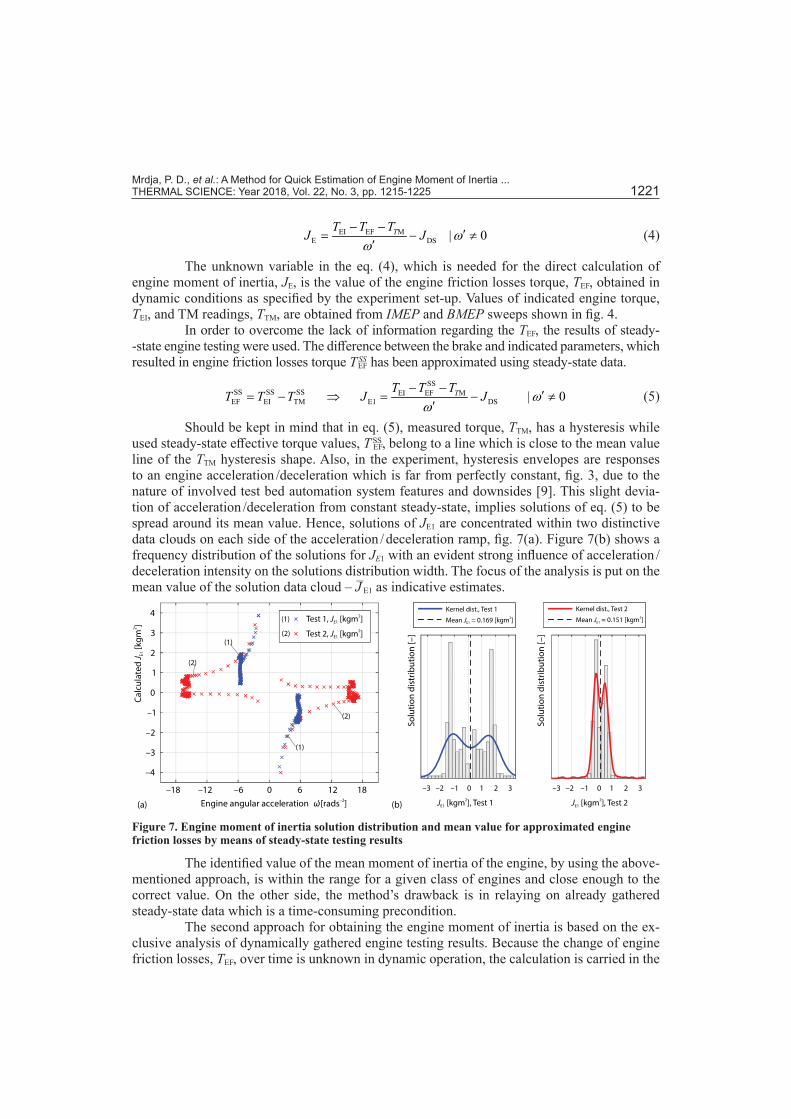
Should be kept in mind that in eq. (5), measured torque, TTM, has a hysteresis while used steady-state effective torque values, T SS

EF, belong to a line which is close to the mean value line of the TTM hysteresis shape. Also, in the experiment, hysteresis envelopes are responses to an engine acceleration /deceleration which is far from perfectly constant, fig. 3, due to the nature of involved test bed automation system features and downsides [9]. This slight devia-tion of acceleration /deceleration from constant steady-state, implies solutions of eq. (5) to be spread around its mean value. Hence, solutions of JE1 are concentrated within two distinctive data clouds on each side of the acceleration / deceleration ramp, fig. 7(a). Figure 7(b) shows a frequency distribution of the solutions for JE1 with an evident strong influence of acceleration /deceleration intensity on the solutions distribution width. The focus of the analysis is put on the mean value of the solution data cloud – J ̄E1 as indicative estimates.

Engine angular acceleration ’ [rads ]–2

ω

–18 –12 –6 0 6 12 18

–4

–3

–2

–1

0

1

2

3

4

(a) (b)

Ca

lcu

late

d[k

gm

]J E

1

2

Test 1, [kgm ]JE1

2

Test 2, [kgm ]JE1

2

JE1

2Test 1[kgm ], JE1

2Test 2[kgm ],

So

luti

on

dis

trib

uti

on

[–

]

So

luti

on

dis

trib

uti

on

[–

]

Kernel dist., Test 1

Mean = 0.169 [kgm ]JE1

2

Kernel dist., Test 2

Mean = 0.151 [kgm ]JE1

2

–3 –2 –1 0 1 2 3 –3 –2 –1 0 1 2 3

(1)

(1)

(2)

(2)

(2)

(1)

ω

Figure 7. Engine moment of inertia solution distribution and mean value for approximated engine friction losses by means of steady-state testing results

The identified value of the mean moment of inertia of the engine, by using the above-mentioned approach, is within the range for a given class of engines and close enough to the correct value. On the other side, the method’s drawback is in relaying on already gathered steady-state data which is a time-consuming precondition.

The second approach for obtaining the engine moment of inertia is based on the ex-clusive analysis of dynamically gathered engine testing results. Because the change of engine friction losses, TEF, over time is unknown in dynamic operation, the calculation is carried in the


opposite direction. In this case, the engine moment of inertia was iteratively assumed and then the dynamic friction losses were calculated. Additional assumptions were included, such as that the change of engine friction losses does not depend on the engine angular acceleration, which is shown in eq. (6): ( )EFT f ω′≠ (6)

Figure 8 shows the change of the calculated dynamic friction mean effective pressure (FMEP), and its smoothing spline approximation, in time and engine speed domain for the conducted dynamic tests and assumed the engine moment of inertia JEA = 0 kgm2. In that sense, predicted FMEP is calculated using eq. (7) and taking into account previous assumptions and engine displacement VE dm3:

( )predicted EA DSE 25

FMEP IMEP BMEP J JV

ω π′= − − + (7)

This value is incorrectly selected with the intention of presenting its impact on TEF results. The presence of FMEP hysteresis is noticeable in the fig. 8 (b) and it is in direct relation with the engine angular accelerations and deceleration periods during the tests. The condition described in eq. (6) provide further analysis based on the approximation of dynamic FMEP over the engine angular speed. In other words, the minimization of the sum of square error (SSE) of the mentioned approximation would lead to the correct result.

Time [sec]0 10 20 30 40 50 60

0

0.5

1

1.5

2

2.5

Pred. Test 1FMEP,

Pred. Test 2FMEP,

Appox. Test 1FMEP,

Approx. Test 2FMEP,

(a)

Assumed "low"

= 0 [kgm ]JEA

2

Engine speed [min ]–1

1000 1500 2000 2500 3000 35000

0.5

1

1.5

2

2.5

Pred. Test 1FMEP,

Pred. Test 2FMEP,

Appox. Test 1FMEP,

Approx. Test 2FMEP,

'<0

'>0

(b)

0 10 20 30 40 50 600

0.5

1

1.5

2

2.5

Pred. Test 1FMEP,

Pred. Test 2FMEP,

Appox. Test 1FMEP,

Approx. Test 2FMEP,

(c)1000 1500 2000 2500 3000 35000

0.5

1

1.5

2

2.5

Pred. Test 1FMEP,

Pred. Test 2FMEP,

Appox. Test 1FMEP,

Approx. Test 2FMEP,

ω’ < 0

(d)

Pre

dic

ted

an

d a

pp

roxi

ma

ted

[ba

r]F

ME

P

Pre

dic

ted

an

d a

pp

roxi

ma

ted

[ba

r]F

ME

P

Assumed "low"

= 0 [kgm ]JEA

2

Pre

dic

ted

an

d a

pp

roxi

ma

ted

[ba

r]F

ME

P

Pre

dic

ted

an

d a

pp

roxi

ma

ted

[ba

r]F

ME

P

Assumed "high"

= 0.3 [kgm ]JEA

2

Time [sec]

Assumed "high"

= 0.3 [kgm ]JEA

2

Engine speed [min ]–1

ω’ > 0

Figure 8. Estimated dynamic FMEP for various assumptions of engine moment of inertia; too low / high in time (a / c) and speed domain (b / d) (for color image see journal web site)


A similar case is presented in figs. 8(c) and 8(d), except that anoth-er extreme value of too high assumed engine moment of inertia is chosen. It is evident that the calculated values for FMEP within dynamic conditions have the opposite direction for positive and negative engine speed slopes com-paring with fig. 8(b).

Beside introduction and eval-uation of approximation error, good indicator of correctly selected engine inertia could be drawn out from hyster-esis area calculation. Minimisation of hysteresis area, which is shown in the figs. 8 and 9, will lead to flip-point of predicted FMEP lines for positive and negative angular accelerations. Results obtained by those two approaches are very similar, but additional data manipulation is required because of unequal data sampling in the engine speed domain. In addition, the iterative estimation of engine moment of inertia is performed and the change of dynamic FMEP smoothing spline approximation SSE is given in fig. 9 for both conducted tests.

It can be noticed that the best fit of FMEP during transient engine speed change cor-responds to a minimal value of SSE which is calculated using eq. (8):

( ) 2

EA predicted aprox1

( ) ( )NS

sSSE J FMEP s FMEP s

=

= − ∑ (8)

where NS represent the total number of samples during the experiment.

Experimental results comparison with CAD model evaluation

For the purpose of results validation, a detailed CAD model of main engine rotation-al elements was made. Engine component masses and their corresponding moment of inertia are presented in the tab. 3. However, it should be noted that the total value is slightly underestimated because el-ements such as the camshaft, pulleys, common rail fuel pump, alternator, the coolant pump impeller and various belts were not modelled.

Described experimental estima-tion of the engine moment of inertia takes into account the influence of en-gine fluids’ inertia (coolant, oil, intake air and exhaust gas-flow in the dynamic condition) which is in non-linear rela-tion to the engine speed and thus not presented in eqs. (5) or (7). In order to provide more accurate results, obtained estimations should be corrected having

No

rma

lize

d d

yn

am

ica

pp

rox.

an

dF

ME

PS

SE

dy

na

mic

hys

tere

sis

are

aF

ME

P

0 0.05 0.1 0.15 0.2 0.25 0.3

Assumed engine mass moment of inertia [kgm ]2

Dyn. approx. Test 1FMEP SSE,

Dyn. approx. Test 2FMEP SSE,

Dyn. hyst. area Test 1FMEP SSE,

Dyn. hyst. area Test 2FMEP SSE,

Min. values, = 0.170 kgm , Test 1JE

2

Min. values, = 0.155 kgm , Test 2JE

2

Figure 9. The SSE of FMEP approximation in dynamic conditions and the minimal value of SSE indicates a correct estimation of engine moment of inertia (for color image see journal web site)

Table 3. Moment of inertia of main engine elements gathered from CAD models

Engine part name Engine part mass [g]

Engine part moment of inertia [kgm2]

Crankshaft 12940 0.0192Flywheel 7960 0.0742

Flywheel-drive shaft adapter 2800 0.0258

Connecting rod mass reduced to the

crankpin journal361.9 0.0024

(all 4 cylinders)

Inertia of the crankshaft mechanism

oscillating parts

0.0022 (all 4 cylinders)

Poly-V pulley 2070 0.0069Total 0.1307


in mind the abovementioned statement. When compared to the CAD model based calculation it is evident that the dynamically estimated inertia is a bit higher with offsets dependable on engine speed ramp. These offsets could be designated:

*

E1 E1*

E2 E2

J J JJ J J

∆

∆

= −

= − (9)

where J* represents the correct value of the engine inertia, and indexes 1 and 2 are related to the slower and faster engine speed gradient, respectively.

By assuming that offsets from eq. (9) are related to the inertia of engine fluids’ mass--flow and internal discharge losses and by using some analogies from the fundamental fluid mechanics equations we can also assume the correctness of the following relation:

E1 2 2

E2 11

QJ kJ kQ

∆∆

≈ ≈ (10)

where Q̄ represents the mean value of the engine fluids’ flow during the acceleration ramp and k accompanying engine speed ramp gradient.

System of eqs. (9) and (10) have a single pair of solutions for the correction offsets:

( ) 2

E1 E21

E2

1

1

1

kJ Jk

Jk

k

− +

∆ =

−

(11)

For the parameters used in the experiment, where k1 and k2 were, respectively, 5.59 and 16.06 rad / s2 and initial estimations of the engine inertia were (from fig. 12) JE1 = 0.170 and JE2 = 0.155 kgm2, the offset resulting from the equation 11 is ΔJE2 = 0.0216 kgm2 which in turn provides a more accurate estimation of the mean engine moment of inertia:

* 2E2 E2 0.133kgmJ J J= − ∆ = (12)

Corrected estimation from eq. (12) is in very good agreement with the CAD based estimation which implies that short transient dynamic measurement can provide the value of engine inertia with remarkable accuracy.

Conclusion

Two methods for experimental estimation of the engine’s moment of inertia are pre-sented in this paper, where both of them are tested with two different engine operation cycles. The first approach presupposes knowledge of engine friction losses values from steady-state operating points, assuming that those values are identical during stationary and dynamic engine examination. The second approach requires far less data and thus, less time on the engine test bed. The assumption that was introduced implies that the value of engine friction losses during dynamic tests does not depend on engine angular acceleration. Results obtained using the sec-ond approach differs between 0.5% and 2.5% compared with the results of the first one. These deviations would be much smaller that the experiment was repeated several times. An intro-duction of an additional method for the correction of engine speed dependable non-linearities provided the final estimation of the mean engine inertia in a very good agreement with the CAD based model estimation. General recommendation for this type of experiment is to vary engine


speed as fast as possible in order to achieve higher inertia inducted torques, taking into account the acceleration that the engine can handle and required dynamometer power for such a run.

Nomenclature

References[1] Perez, F., et al., Vehicle Simulation on an Engine Test Bed, Proceedings, SIA International Conference,

Diesel Engines – The Low CO2 & Emissions Reduction Challenge, 2008[2] Burette, G., et al., Vehicle Calibration Optimization Using a Dynamic Test Bed with Real Time Vehicle Sim-

ulation, Proceedings, Diesel Engines - Facing the Competitiveness Challenges, Campus INSA de Rouen, France, 2010

[3] Isermann, R., Engine Modeling and Control: Modeling and Electronic Management of Internal Combus-tion Engines, Springer, New York, USA, 2014

[4] Zweiri, Y. H., et al., Detailed Analytical Model of a Single-Cylinder Diesel Engine in the Crank Angle Domain, Journal of Automobile Engineering, 215, (2001), 11, pp. 1197-216

[5] Souflas, I., et al., Dynamic Modeling of a Transient Engine Test Cell for Cold Engine Testing Applica-tions, Proceedings, ASME 2014 International Mechanical Engineering Congress and Exposition, ASME, Montreal, Que., Canada, 2014

[6] Mrdja, P., Integrated Solution for Internal Combustion Engine Test Bench Control, Data Acquisition and Engine Control Unit Calibration, Proceedings, NIDays 2011 International Conference, Belgrade, 2011

[7] Paulweber, M., Lebert, K., Powertrain Instrumentation and Test Systems: Development – Hybridization – Electrification, Springer, New York, USA, 2016

[8] *** AVL Indicom Indicating Software v1.6. AVL List GmbH, Graz, Austria [9] Dinić, S., et al., Light Vehicles Test Procedures on an Automated Engine Test Bed, Proceedings, 17th Sym-

posium on Thermal Science and Engineering of Serbia, Sokobanja, Serbia, 2015, pp. 1056-1061 [10] Petrović, V., et al., Software and Hardware Challenges of Engine Test Bed Automation – Example of

FME ICED Lab, Proceedings, 17th Symposium on Thermal Science and Engineering of Serbia, Sokoban-ja, Serbia, 2015, pp. 1062-1065

[11] Godburn, J., et al., Computer-Controlled Non-Steady-State Engine Testing, International Journal of Ve-hicle Design, 12 (2001 ) 1, pp. 50-60

[12] Schreiber, A., Dynamic Engine Measurement with Various Methods and Models, (in German), in Elec-tronic Management of Motor Vehicle Powertrains, Springer, Berlin, German, 2010, pp. 167-199

[13] Ward, M. C., et al., Investigation of Sweep Mapping Approach on Engine Testbed, Proceedings, SAE 2002 World Congress & Exhibition, Detroit, Mich., USA, 2002

Paper submitted: September 15, 2017Paper revised: October 16, 2017Paper accepted: October 24, 2017

© 2018 Society of Thermal Engineers of SerbiaPublished by the Vinča Institute of Nuclear Sciences, Belgrade, Serbia.

This is an open access article distributed under the CC BY-NC-ND 4.0 terms and conditions

J – moment of inertia, [kgm2]k – acceleration /deceleration ramp gradientNS – number of samplesQ – equivalent fluid-flow of all engine fluidsT – torque, [Nm]V – volume, [dm3]

Greek symbols

Δ – differenceω – angular speed, [rads–1]ωʹ – angular acceleration, [rads–2]

Subscripts

D – dynamometerDB – dynamometer brakeDF – dynamometer frictionDS – drive shaftE – engineEF – engine frictionEI – engine indicatedTM – torque meter

Superscrips

* – new valueSS – steady-state

A METHOD FOR QUICK ESTIMATION OF ENGINE MOMENT OF …

Documents

Transcript of A METHOD FOR QUICK ESTIMATION OF ENGINE MOMENT OF …