A method for quantifying, visualising, and analysing gastropod shell
51
A method for quantifying, visualising, and analysing gastropod shell form Quantitative analysis of organismal form is an important component for almost every branch of biology. Although generally considered an easily-measurable structure, the quantification of gastropod shell form is still a challenge because shells lack homologous structures and have a spiral form that is difficult to capture with linear measurements. In view of this, we adopt the idea of theoretical modelling of shell form, in which the shell form is the product of aperture ontogeny profiles in terms of aperture growth trajectory that is quantified as curvature and torsion, and of aperture form that is represented by size and shape. We develop a workflow for the analysis of shell forms based on the aperture ontogeny profile, starting from the procedure of data preparation (retopologising the shell model), via data acquisition (calculation of aperture growth trajectory, aperture form and ontogeny axis), and data presentation (qualitative comparison between shell forms) and ending with data analysis (quantitative comparison between shell forms). We evaluate our methods on representative shells of the genus Opisthostoma, which exhibit great variability in shell form. The outcome suggests that our method is more robust, reproducible, and versatile than the conventional traditional and geometric morphometric approaches for the analysis of shell form. Finally, we propose several potential applications of our methods in functional morphology, theoretical modelling, taxonomy, and evolutionary biology. PeerJ PrePrints | https://peerj.com/preprints/157v1/ | v1 received: 16 Dec 2013, published: 16 Dec 2013, doi: 10.7287/peerj.preprints.157v1 PrePrints
Transcript of A method for quantifying, visualising, and analysing gastropod shell

A method for quantifying, visualising, and analysing gastropod shell form
Quantitative analysis of organismal form is an important component for almost every branch
of biology. Although generally considered an easily-measurable structure, the quantification
of gastropod shell form is still a challenge because shells lack homologous structures and
have a spiral form that is difficult to capture with linear measurements. In view of this, we
adopt the idea of theoretical modelling of shell form, in which the shell form is the product of
aperture ontogeny profiles in terms of aperture growth trajectory that is quantified as
curvature and torsion, and of aperture form that is represented by size and shape. We
develop a workflow for the analysis of shell forms based on the aperture ontogeny profile,
starting from the procedure of data preparation (retopologising the shell model), via data
acquisition (calculation of aperture growth trajectory, aperture form and ontogeny axis), and
data presentation (qualitative comparison between shell forms) and ending with data analysis
(quantitative comparison between shell forms). We evaluate our methods on representative
shells of the genus Opisthostoma, which exhibit great variability in shell form. The outcome
suggests that our method is more robust, reproducible, and versatile than the conventional
traditional and geometric morphometric approaches for the analysis of shell form. Finally, we
propose several potential applications of our methods in functional morphology, theoretical
modelling, taxonomy, and evolutionary biology.
PeerJ PrePrints | https://peerj.com/preprints/157v1/ | v1 received: 16 Dec 2013, published: 16 Dec 2013, doi: 10.7287/peerj.preprints.157v1
PrePrin
ts

Thor-Seng Liew and Menno Schilthuizen
1 Institute Biology Leiden, Leiden University, P.O. Box 9516, 2300 RA Leiden, The Netherlands.
2 Naturalis Biodiversity Center, P.O. Box 9517, 2300 RA Leiden, The Netherlands.
3 Institute for Tropical Biology and Conservation, Universiti Malaysia Sabah, Jalan UMS, 88400,
Kota Kinabalu, Sabah, Malaysia.
Email: T-S L: [email protected]
Funding: This study is funded under project 819.01.012 of Research Council for Earth and Life
Sciences (ALW-NOW). The funders had no role in study design, data collection and analysis,
decision to publish, or preparation of the manuscript.
Competing interests: The authors have declared that no competing interests exist.
Introduction
Empirical and theoretical approach in the study of shell form
1
2
3
4
5
6
7
8
9
10
11
12
13
PeerJ PrePrints | https://peerj.com/preprints/157v1/ | v1 received: 16 Dec 2013, published: 16 Dec 2013, doi: 10.7287/peerj.preprints.157v1
PrePrin
ts

The external form diversity of organisms is the most obvious evidence for their evolution, and
thus is a key element in most branches of biology. The Molluscan shell has been a popular
example in morphological evolution studies because it is geometrically simple, yet diverse in
form. The shell form is controlled by the shell ontogenetic process, which follows a simple
accretionary growth mode where new shell material is accumulatively deposited to the existing
aperture. The evolution of shell forms has been studied either by using empirical approaches that
focus on the quantification of actual shell forms or by using theoretical approaches that focus on
the simulation of shell ontogenetic processes and geometric forms.
Notwithstanding the active development in both empirical and theoretical approaches to the study
of shell form, there has been very little integration between both schools. For the empirical
approach, the quantification methods of shell form have evolved from traditional linear
measurement to landmark-based geometric morphometrics and outline analyses (for an overview
see Van Bocxlaer & Schultheiß, 2010). At the same time, for the theoretical approach, the
simulations of shell form have evolved from simple geometry models that aimed to reproduce the
form, to more comprehensive models that simulate shell ontogenetic processes (for an overview
see Urdy et al., 2010). Hence, each of the two approaches has been moving forward but away
from each other, where synthesis between the two schools of shell morphologists has become
more challenging.
In empirical morphological studies, shell form, either in terms of heights and widths in traditional
morphometrics or in terms of geometry of procrustes distances in geometric morphometrics, is
quantified by a set of homologous reference points or landmarks on the shell, which can be easily
obtained from the fixed dimensions of the shell. Thus, both methods could abstract the shell form
in terms of size and shape of the particular shell dimensions, and the between-sample variation of
shell size and shape can be assessed (in most cases only within one study). On the other hand, it
is not possible to reconstruct the actual shell form from these quantitative measurements, because
the shell’s accretionary growth model and spiral geometry cannot be quantified on the basis of
arbitrary reference points or fixed dimensions (Stone. 1997). Nevertheless, the traditional and
geometric morphometric methods have been accepted widely as standard quantification methods
for shell form in many different fields of research.
14
15
16
17
18
19
20
21
22
23
24
25
26
27
28
29
30
31
32
33
34
35
36
37
38
39
40
41
42
PeerJ PrePrints | https://peerj.com/preprints/157v1/ | v1 received: 16 Dec 2013, published: 16 Dec 2013, doi: 10.7287/peerj.preprints.157v1
PrePrin
ts

In contrast to empirical morphometrics in which the aim is to quantify the actual shell, theoretical
morphologists focus on the simulation of an accretionary growth process which produces a shell
form that is similar to actual shells. This field was established with the theoretical shell model of
D.M. Raup (Raup, 1961; Raup & Michelson, 1965). Within the first two decades after these
publications, only a few different versions of shell models were proposed (e.g. Løvtrup & von
Sydow, 1974; Bayer, 1978; McGhee, 1978; Kawaguchi, 1982; Illert, 1983). The subsequent two
decades, thanks to the popularity and power of desktop computing, many more theoretical shell
models were published (e.g., Savazzi, 1985; Okamoto, 1988; Cortie, 1989; Ackerly, 1989a;
Savazzi, 1990; Checa, 1991; Fowler et al., 1992; Illert & Pickover, 1992; Checa & Aguado, 1992;
Cortie, 1993; Savazzi, 1993; Rice, 1998; Ubukata, 2001; Galbraith, Prusinkiewicz & Wyvill,
2002). Finally, we saw further improvements in the published theoretical models in recent years.
These recent models simulate shell forms that more accurately resemble actual shells because of
improved programming software, better algorithms, and 3D technology (e.g. Picado, 2009,
Stępień, 2009; Meinhardt, 2009; Urdy et al., 2010; Harary & Tal, 2011; Moulton & Goriely,
2012; Moulton, Goriely & Chirat, 2012; Faghih Shojaei et al., 2012; Chacon, 2012). Here, we
will not further discuss the details of the at least 29 published shell models, but refer to the
comprehensive overviews and descriptions of these models in Dera et al. (2009) and Urdy et al.
(2010).
In brief, the latest theoretical shell models are able to simulate irregularly-coiled shell forms and
ornamentations that resemble actual shells, whereas the earlier models could only simulate the
regular and general shape of shells. The major refinements that have been made during the almost
five decades’ development of theoretical shell models are the following modifications of the
algorithm: 1) from a fixed reference frame to a moving reference frame system; 2) from
modelling based on numerical geometry parameters to growth-parameter-based modelling (e.g.
growth rates); 3) from three parameters to more than three parameters, which has made fine-
tuning of the shell simulation (e.g. aperture shape) possible. The key element of the theoretical
modelling of shells is the generation of shell form by simulating the aperture ontogeny in terms
of growth trajectory and form along the shell ontogeny. Hence, this has an advantage over the
empirical approach in the numerical representation of the shell geometry form in terms of the 3D
quantification and the actual shell ontogenetic processes.
43
44
45
46
47
48
49
50
51
52
53
54
55
56
57
58
59
60
61
62
63
64
65
66
67
68
69
70
71
72
PeerJ PrePrints | https://peerj.com/preprints/157v1/ | v1 received: 16 Dec 2013, published: 16 Dec 2013, doi: 10.7287/peerj.preprints.157v1
PrePrin
ts

Since the empirical and theoretical researchers studying shell form with two totally different
quantification methods, our understanding of shell evolution cannot progress solely by using
either empirical morphometrics or theoretical models. Ideally, theoretical models need to be
evaluated by empirical data of shell morphometrics, and, vice-versa, empirical morphometric
methods need to be improved to obtain data that better reflect the actual shell form and
morphogenesis which can then be used to improve the theoretical models. In this dilemma lies
the central problem of shell form quantification and it urgently needs to be addressed in order to
integrate and generalise studies of shell form evolution.
Why empirical morphologists rarely use theoretical shell models
Despite the fact that, since the 1980s, manyshell models have been published that are more
complex and versatile, the first theoretical shell model of Raup still remains the most popular.
There were many attempts by empirical morphologists to use the original or a modified version
of Raup’s parameters to quantify natural shell forms (e.g. Raup, 1967; Vermeij, 1971; Davoli &
Rosso, 1974; Graus, 1974; Kohn & Riggs, 1975; Newkirk & Doyle, 1975; Warburton, 1979;
Verduin, 1982; Ekaratne & Crisp, 1983; Saunders & Shapiro, 1986; Tissot, 1988; Foote & Cowie,
1988; Johnston, Tabachnick & Bookstein, 1991; Emberton, 1994; Clarke, Grahame & Mill, 1999;
Samadi, David & Jarne, 2000). Surprisingly, all the other shell models, many of which produce
more realistic forms, have received very little attention as compared to Raup’s model (see e.g.
Savazzi, 1992; Okajima & Chiba, 2011; Okajima & Chiba, 2012, for exceptions). This ironic
situation might be explained by the elegance of Raup’s model that is intuitively and
mathematically simple to be used by empirical morphologists (mostly biologists), with limited
mathematical and programming experience.
As discussed above, most of the theoretical models can simulate a shell that has a form
resembling the actual shell in a realistic 3D geometry, based on shell ontogeny processes. In
contrast, empirical morphometrics can only quantify and compare certain dimensions of actual
shells. Clearly, the theoretical approach is better than the empirical approach in its accuracy of
shell form quantification, because accurate morphological quantification is essential for
functional, ecological and evolutionary studies of shell form. Below, we identify and discuss a
few impediments that currently prevent empirical morphologists from adopting the theoretical
approach in shell form quantification.
73
74
75
76
77
78
79
80
81
82
83
84
85
86
87
88
89
90
91
92
93
94
95
96
97
98
99
100
101
102
PeerJ PrePrints | https://peerj.com/preprints/157v1/ | v1 received: 16 Dec 2013, published: 16 Dec 2013, doi: 10.7287/peerj.preprints.157v1
PrePrin
ts

First, the requirement of a computation resource was an impediment in the past. These theoretical
models may only be implemented in a computation environment. As mentioned above, the
advances of computation hardware in speed and 3D graphic technology have promoted the
development of more complex theoretical shell models. For example, the current speed and
storage of a desktop computer is at least four orders of magnitude greater than those used by
Cortie (1993) only two decades ago. Clearly, the computation hardware is no longer an
impediment (e.g. Savazzi, 1995) for the application and development of theoretical shell models.
Notwithstanding the hardware development, programming skills are still a prerequisite for the
implementation of theoretical models. Many of the early models that were published between the
1960s and 1990s, used third-generation programming languages such as Fortran and C++, which
essentially lack a graphic user interface. This situation has improved now that the simulation of
theoretical shell models can be done in fourth-generation programming languages such as
Mathematica (e.g. Meinhardt, 2009; Noshita, 2010; Okajima & Chiba, 2011; Okajima & Chiba,
2012) and MATLAB (e.g. Boettiger, Ermentrout & Oster, 2009; Urdy et al. 2010, Faghih Shojaei
et al., 2012). Most of these shell models were described with intensive mathematical notation, at
least from a biologist’s point of view, in the publication; and some of these were published
together with the information on algorithm implementation. However, the actual programming
codes are rarely published together with the paper though they may be available from the authors
upon request (but see Meinhardt, 2009; Noshita, 2010; Okajima & Chiba, 2011). Only one
theoretical modelling software package based on Raup’s model has a graphic user interface that is
comparable to contemporary geometric morphometric software (Noshita, 2010). Thus, the rest of
the modern theoretical models are far less approachable than the morphometric software for
empirical morphologists. This is because those advanced theoretical models have not been
delivered in a form that allowed empirical morphologists to have “hands-on experience” with
them, without extensive mathematical literacy (Savazzi, 1995; McGhee, 2007).
Second, theoretical shell models simulate the shell form based on the input of a set of parameters,
which could be non-biological or/and biologically meaningful. Non-biological meaningful
parameters are counter-intuitive for empirical morphologists because these parameters are not
extrinsic shell traits. Nevertheless, many of these non-biological parameters are required for the
model to fit the shell form schematically (Hutchinson, 1999). When the biological parameters do
103
104
105
106
107
108
109
110
111
112
113
114
115
116
117
118
119
120
121
122
123
124
125
126
127
128
129
130
131
132
PeerJ PrePrints | https://peerj.com/preprints/157v1/ | v1 received: 16 Dec 2013, published: 16 Dec 2013, doi: 10.7287/peerj.preprints.157v1
PrePrin
ts

represent shell traits, they are often difficult to obtain accurately and directly from the actual shell
because of the three-dimensional spiral geometry (Cain, 1977; Ackerly, 1989a; Ackerly, 1989b;
Okamoto, 1988; Schindel, 1990; Checa & Aguado, 1992, Hutchinson, 1999; McGhee, 1999).
Since the development of theoretical shell models, almost all simulated shell models have been
made by an ad hoc approach, where the parameters are chosen for the model and then the
simulated shells are compared with the actual shells. In almost all cases, the correct parameters
are chosen after a series of trial-and-error, and the parameters are selected when the form of the
simulated shell matches the actual shell. Okamoto (1988) suggested that this ad hoc approach
based on pattern matching was easier than obtaining the parameters empirically from the shell.
Third, although the overall forms of the simulated shells resemble the actual shells, the simulated
shell is not exactly the same as the actual shell (Kohn & Riggs, 1975; Goodfriend, 1983). For
many models, its original parameters are not sufficient to simulate the shell form exactly
(Schindel, 1990; Fowler, Meinhardt & Prusinkiewicz, 1992). These simulated general shell forms
are adequate for theoretical morphologist interests in their exploration of general shell forms.
However, the subtle features on a real shell or the subtle differences among different shell forms
of real species that cannot be simulated by theoretical models may have significant functional
implications that are important for empirical morphologists.
In brief, it is clear that the implementation of current theoretical shell models is less accessible to
empirical shell morphologists. Yet, empirical morphologists are using traditional and geometric
morphometrics as a routine method for shell quantification.
Why empirical morphologists use traditional and geometric morphometrics
In addition to the impediments arising from the theoretical shell model itself that are limiting its
popularity among empirical morphologists, the theoretical approach faces competition from
geometric morphometric methodology. The popularisation of desktop computing that led to the
flourishing of theoretical shell models in the late 1980s, also promoted the development of
morphometric methods, such as Elliptical Fourier Analysis (EFA) and geometric morphometrics
(GM). Rohlf and Archie (1984) set a benchmark for the quantification of an organism’s form by
EFA, which was improved from Kaesler and Waters (1972) and Kuhl and Giardina (1982). Rohlf
and Slice (1990) and Bookstein (1991) developed a complete standard protocol for GM. Soon
133
134
135
136
137
138
139
140
141
142
143
144
145
146
147
148
149
150
151
152
153
154
155
156
157
158
159
160
161
PeerJ PrePrints | https://peerj.com/preprints/157v1/ | v1 received: 16 Dec 2013, published: 16 Dec 2013, doi: 10.7287/peerj.preprints.157v1
PrePrin
ts
after these pioneer papers, various software with Graphic User Interface (GUI) were developed
for the application of EFA and GM (Cardini & Loy, 2013, see http://life.bio.sunysb.edu/morph/).
In contrast to the application of theoretical shell models, an understanding of mathematics and
programming languages is not a prerequisite for the user of these morphometric tools. Thus, EFA
and GM have been well received by biologists, and have been adopted in the morphometric study
of shell form.
These geometric morphometric software packages have standard and interactive workflows that
help empirical morphologists in every step of: obtaining morphometric data (e.g. placing
landmark coordinates), analysing data (e.g. procrustes superimposition), statistical analysis (e.g.
ANOVA, PCA), and visualising shape and shape changes (e.g. thin-plate spline, PCA plots). This
has made geometric morphometrics approachable and attractive to empirical morphologists, who
want to examine the similarities and differences among shell forms.
Geometric morphometrics is actually a statistic of shape that is calculated from Cartesian
coordinate data from a sample of objects (Cardini & Loy, 2013). However, it is not an exact
quantification of form and is not particularly suitable for comparison and quantification of shell
form, for the following two reasons.
First, GM analysis is based on homologous landmarks on the form, but shell has only arbitrary
landmarks because it has a low degree of morphological complexity (Van Bocxlaer & Schultheiß
2010). In most cases, 2D landmarks are chosen at the shell apex, suture, and aperture or whorl
outline that can be identified from a 2D image that is taken in standard apertural view of a shell.
These landmarks are chosen to be analysed by GM but these points have little biological
meaning. Furthermore, as opposed to the form of many other organisms, 3D landmarks are even
more difficult to be obtained from a shell (3D model) as compared to 2D landmarks because
many of these landmarks, such as suture points, that are obtained from a 2D image are just
artefacts of the fixed 2D view of the shell.
Second, the results of separate, independent studies of shell forms cannot be integrated, even
though these studies use the same GM method. Statistical analysis of the Cartesian coordinate
data that abstractly represent the shell form is adequate in quantifying the variation of a shell
within a context of other shells that are included in a single study or within similar taxa where
162
163
164
165
166
167
168
169
170
171
172
173
174
175
176
177
178
179
180
181
182
183
184
185
186
187
188
189
190
PeerJ PrePrints | https://peerj.com/preprints/157v1/ | v1 received: 16 Dec 2013, published: 16 Dec 2013, doi: 10.7287/peerj.preprints.157v1
PrePrin
ts
similar landmarks are obtained. However, the raw coordinate data and analysed shape variation
from a study are incomparable and incompatible with the data from other studies (Klingenberg,
2013).
Despite the fact that geometric morphometrics has been widely used by empirical morphologists,
it is not an ideal tool in the quantification of shell form for the reasons given above. The
increasing availability of the software and application in the literature might cause morphologists
to stray away from their initial aims of studying shell form. Hence, it is important to return to the
core of the question: what do biologists want to learn from the study of shell form? Clearly, in
addition to quantitatively compare shell forms, biologists want to know more about the general
characteristics and physical properties of the shell form that are key elements in gaining insight
into functional and ecological aspects of the shell (Evans, 2013). However, functional and
ecological aspects of shell form can only be determined if the shell form can be exactly
quantified.
Using 3D technology to quantify shell form based on aperture ontogeny profiles
In this paper, we propose an interactive approach to the quantification and analysis of shell forms
based on state of the art 3D technology and by integrating the theoretical principles of shell
modelling and the empirical principles of morphometric data handling. There are no theoretical
models that can simulate all existing shell forms. However, the theoretical background of the
theoretical models is biologically sound – simulating the shell form by simulating the shell
ontogenetic process. On the basis of this shell-ontogenesis principle, we used state-of-the-art X-
ray microtomography (micro-CT scan) and 3D modelling software to obtain a series of shell
aperture changes from the shell in an interactive workflow that is similar to empirical
morphometric analysis.
First, a series of shell aperture outlines were digitised directly from the reconstructed 3D shell
model obtained from micro-CT scanning by using open-source 3D-modelling software – Blender
ver. 2.63 (www.blender.org). Then, the growth trajectory and form of the shell aperture outline
were quantified and extracted with our custom scripts that run in Blender through its embedded
open-source Python interpreter (http://www.python.org/). The changes of aperture size and shape,
and aperture growth trajectory in terms of curvature and torsion along the shell ontogeny axis
191
192
193
194
195
196
197
198
199
200
201
202
203
204
205
206
207
208
209
210
211
212
213
214
215
216
217
218
219
PeerJ PrePrints | https://peerj.com/preprints/157v1/ | v1 received: 16 Dec 2013, published: 16 Dec 2013, doi: 10.7287/peerj.preprints.157v1
PrePrin
ts

length were obtained (hereafter “aperture ontogeny profiles”). The final aperture ontogeny
profiles are in a form of multivariate time series data, which consist of a number of instances (i.e.
number of quantified apertures that depends on the length of the whorled shell tube) and
attributes that represent the growth trajectories, aperture form, and size.
These aperture ontogeny profiles can be plotted when each shell is examined individually. On the
other hand, the aperture ontogeny profiles can be visually compared between different shells by
plotting the data as radar chart (i.e. spider and star plots). In addition, the differences between
shells can be assessed quantitatively by calculating the dissimilarity of aperture ontogeny profiles
among shells. Furthermore, the dissimilarity matrix can be used to plot the dendrogram and
NMDS plots, which resemble a shell morphospace. All our procedures were implemented by
using open source and free software.
Finally, we discuss some possible applications and implications of these shell form quantification
methods in theoretical morphology, functional morphology, taxonomy and shell shape
evolutionary studies.
Materials and Methods
Ethics Statement
Specimens were collected in Malaysia with permissions from the Economic Planning Unit,
Malaysia (UPE: 40/200/19/2524).
Scanning instrumentation
A micro-CT scanner (SkyScan, model 1172, Aartselaar, Belgium) and its accompanying software,
NRecon ver. 1.6.6.0 (Skyscan©) and CT Analyser ver. 1.12.0.0 (Skyscan©), were used to
generate digital shell 3D models from the actual shell specimens.
Computation software and hardware
Various commercial 3D modelling and statistical software exist for visualising, manipulating, and
understanding morphology, such as Amira® (Visage Imaging Inc., San Diego, CA) and Autodesk
Maya (San Rafael, CA) (reviewed by Abel, Laurini & Richter, 2012). However, in this study, we
used only two open-source 3D data modelling and processing software packages, namely Blender
220
221
222
223
224
225
226
227
228
229
230
231
232
233
234
235
236
237
238
239
240
241
242
243
244
245
246
PeerJ PrePrints | https://peerj.com/preprints/157v1/ | v1 received: 16 Dec 2013, published: 16 Dec 2013, doi: 10.7287/peerj.preprints.157v1
PrePrin
ts

ver. 2.63 (www.blender.org) and Meshlab ver. 1.3.2 (Cignoni, Corsini & Ranzuglia, 2008,
http://meshlab.sourceforge.net/). Both have been used in biology to visualise and model
morphology (for Meshlab: Im et al., 2012; Chaplin, Yu & Ros, 2013; Atwood & Sumrall, 2012;
for Blender: Pyka et al., 2010: 22); Haug, Maas & Waloszek, 2009; Cassola et al., 2010; Haug et
al., 2010; Andrei et al., 2012; Haug et al., 2012; Lv et al., 2013; Mayer et al., 2012). However,
these programs have not been used to their full extent in morphological quantification and
analysis of 3D data for organisms. For quantification of morphology, we used the open-source
Python interpreter ver. 3.2 that is embedded in Blender 2.63. In addition, we also used an
extension to the Python programming language – NumPy (Oliphant, 2007) which consists of
high-level mathematical functions.
All the morphological data were explored and analysed with the statistical open source
programming language R version 3.0.1 (R Core Team, 2013) in the environment of RStudio
(RStudio, 2012). We installed three additional packages in R, namely, "lattice": Lattice Graphics
(Sarkar, 2008), "pdc": Permutation Distribution Clustering (Brandmaier, 2012a; Brandmaier,
2012b), and "fmsb" (Nakazawa, 2010).
All the computation analyses were carried out with a regular laptop computer with the following
specifications: Intel®Core™i7-3612QM @ 2.1GHz, 8 GB memory (RAM), NVIDIA® GeForce
GT 630M with 2GB memory.
Procedures
1. Obtaining digital 3D models from actual shells
The scan conditions were as follows: voltage – 80kV or 100kV; pixel – 1336 rows × 2000
columns; camera binning – 2 × 2; image pixel size – 3–6 μm; rotation step – 0.4° or 0.5°; and
rotation – 360°. Next, the volume reconstruction on the acquired images was done in NRecon.
The images were aligned to the reference scan and reconstruction was done on the following
settings: beam hardening correction – 100%; reconstruction angular range – 360 degree;
minimum and maximum for CS to image conversion (dynamic range) – ca. 0.12 and ca. 20.0; and
result file type – BMP. Finally, 3D models were created from the reconstruction images in CT
Analyser with the following setting: binary image index – 1 to 255 or 70 to 255; and were saved
as digital polygon mesh object (*.PLY format).
247
248
249
250
251
252
253
254
255
256
257
258
259
260
261
262
263
264
265
266
267
268
269
270
271
272
273
274
275
PeerJ PrePrints | https://peerj.com/preprints/157v1/ | v1 received: 16 Dec 2013, published: 16 Dec 2013, doi: 10.7287/peerj.preprints.157v1
PrePrin
ts

2. Pre-processing digital shell models
The 3D models were then simplified by quadric edge collapse decimation implemented in
MeshLab (Cignoni, Corsini & Ranzuglia, 2008) to reduce computation requirements. The raw
polygon mesh shells in PLY format have millions of faces and a file size between 20 to 80
Mbytes. Thus, we reduced the number of faces for all model to 200,000 – 300,000 faces, which
range between 3 and 6 Mbytes in file size. In addition, for the sake of convenience during the
retopology processes, all 3D models were repositioned so that the shell protoconch columella was
parallel with the z-axis. This was done by using manipulator tools in MeshLab.
3. Creating reference: Tracing aperture outlines and ontogeny axis from shell models
The digital shell 3D model in PLY format consists of 3D Cartesian coordinate vertices in which
each of the three vertices constitutes a triangular face, and all faces are connected through a
complex network. In order words, these vertices and faces are not biologically meaningful
structures, and it is not possible to extract aperture outlines data directly from a raw PLY digital
shell model. Monnet et al. (2009), for example, attempted to extract aperture outline
automatically from a digital 3D model by making a plane cross-sectioning of the shell model, but
its outlines do not reflect the form of the actual aperture outlines. Hence, we retopologised the
raw 3D mesh models according to the aperture ontogeny for later data extraction.
We used Blender, which is more flexible than the commercial software used by Monnet et al.
(2009). For the sake of convenience, we describe the following workflow, including the tools or
the function (e.g. “Import PLY”) which can be called after hitting the SPACE bar while in the
Blender environment. However, this workflow may be modified by the user.
To begin, we imported a PLY shell model into the Blender environment (“Import PLY”). Then,
we resized the model 1000 × (“Resize”) so that the scale of 1 Blender unit was equal to 1 mm.
After that, we examined the traces of aperture outlines (i.e. growth lines, ribs, spines) (Figure 1A)
and ontogeny axis (i.e. spiral striation, ridges, colour lines) (Figure 1B) of the actual shells. After
these aperture traits were identified, we selected the 3D model (by clicking “right mouse
button”), and traced all these traits on the surface of the raw 3D mesh model in Blender by using
the “Grease Pen Draw” tool. After that, the grease pen traced aperture traits were converted to
Bezier curves with “Convert Grease Pencil” (Figure 1C).
276
277
278
279
280
281
282
283
284
285
286
287
288
289
290
291
292
293
294
295
296
297
298
299
300
301
302
303
304
PeerJ PrePrints | https://peerj.com/preprints/157v1/ | v1 received: 16 Dec 2013, published: 16 Dec 2013, doi: 10.7287/peerj.preprints.157v1
PrePrin
ts

4. Retopologising aperture outlines from the reference and generating retopologised shell models
For each shell, we created a set of new Non Uniform Rational B-Splines (NURBS) surface
circles (“Add Surface Circle”) and modified these (“Toggle Editmode”) according to the aperture
outlines. We created a 16 points NURBS surface circle and aligned the circle to the aperture
outline by translation (“Translate”), rotation (“Rotate”), and resizing (“Resize”) (Figure 1D).
After the NURBS surface circle was generally aligned, each of the 16 points of the NURBS
surface circle were selected and adjusted by translation (“G”) one by one, so that the outline of
the NURBS surface circle was exactly the same as the aperture outline. At the same time, the
second point of the NURBS surface circle was aligned to the ontogeny axis (Figures 1B and 1C).
After the first aperture outline was retopologised as a NURBS surface circle, the NURBS surface
circle was duplicated (“Duplicate Objects”) and aligned to the next aperture outline as the
previous one. This step was repeated until all the aperture outlines were retopologised into
NURBS surface circles (Figures 1D and 1E). Then the shell surface was created in the form of a
NURBS surface based on the digitised aperture NURBS surface circle (“(De)select All” and
“Make Segment” in “Toggle Editmode”) (Figures 1F and 1G). Lastly, we made the surface meet
the end points in U direction and increased the surface subdivision per segment (resolution U = 8)
through the properties menu of the object (Properties (Editor types)>Object Data>Active Spline).
After that, we converted the NURBS surface 3D model into a 3D Mesh model that consists of
vertices, edges, and faces (“Convert to” - “Mesh from Curve/Meta/Surf/Text”). The final
retopologised 3D shell Mesh consists of X number of apertures outlines and each aperture outline
has Y number of vertices and then a total of X*Y vertices. Each of the vertices is connected to
four other nearest vertices with edges to form a wireframe shell and face (Figure 1H).
It is important to note that the NURBS surface circle is defined by a mathematic formula which
does not imply any biology perspective of the shell. We choose NURBS surface circle because
the 3D aperture outline form can be digitalised by a small number of control points and shell
surface can be recreated by NURBS surface based on the digitised aperture NURBS surface
circle. The final 3D polygon mesh model is more simplified than the raw PLY 3D model and each
of its vertex data resemble the actual accretionary process of the shell (Figures 1A and 1H).
5. Quantifying aperture growth trajectory
305
306
307
308
309
310
311
312
313
314
315
316
317
318
319
320
321
322
323
324
325
326
327
328
329
330
331
332
333
PeerJ PrePrints | https://peerj.com/preprints/157v1/ | v1 received: 16 Dec 2013, published: 16 Dec 2013, doi: 10.7287/peerj.preprints.157v1
PrePrin
ts

The aperture ontogeny profiles were quantified as described in Liew et al. (in press, b) with slight
modifications where both aperture growth trajectory and aperture form were quantified directly
from the retopologised 3D shell model. This aperture growth trajectory was quantified as a spatial
curve, which is the ontogeny axis as represented by a series of first points of the aperture outlines.
We estimated two differential geometry parameters, namely, curvature (κ) torsion (τ), and
ontogeny axis length for all apertures (Okamoto, 1988; Harary & Tal, 2011). The local curvature
and torsion, and accumulative ontogeny axis length were estimated from the aperture points
along the growth trajectory by using weighted least-squares fitting and local arc length
approximation (Lewiner et al., 2005). All the calculations were done with a custom-written
Python script which can be implemented in Python interpreter in the Blender ver. 2.63
environment. The whole workflow was: (1) selecting the retopologised 3D shell Mesh (by
clicking “right mouse button”), (2) input parameters for number of sample points “q = ##” in the
python script, and (3) paste the script into the Python interpreter (Supplementary Information File
1). The final outputs with torsion, curvature and ontogeny axis reference for each aperture were
saved as CSV files.
We found a convergence issue in curvature and torsion estimators. The accuracy of the curvature
and torsion estimates depends on the number and density of the vertices in the ontogeny axis (i.e.
number of aperture outlines), and the number of sample points. Nevertheless, different numbers
of sample points can be adjusted until good (i.e. converged) curvature and torsion estimates are
obtained. We used 10% of the total points as number of sample points of the ontogeny axis,
which gave reasonably good estimates for curvature and torsion.
Notwithstanding the algorithm issue, the curvature and torsion estimators are informative in
describing the shell spiral geometry growth trajectory. Curvature is always larger or equal to zero
(κ ≥ 0). When κ = 0, the spatial curve is a straight line; the larger the curvature, the smaller the
radius of curvature (1/ κ), and thus the more tightly coiled the spatial curve. On the other hand,
the torsion estimator can be zero or take either negative or positive values (- ∞ ≤ τ ≤ ∞). When τ
= 0, the spatial curve lies completely in one plane (e.g. a flat planispiral shell), negative torsion
values correspond to left-handed coiling and to right-handed coiling for positive torsion values;
the larger the torsion, the smaller the radius of torsion (1/ τ), and thus the taller the spiral.
6. Quantifying aperture form
334
335
336
337
338
339
340
341
342
343
344
345
346
347
348
349
350
351
352
353
354
355
356
357
358
359
360
361
362
363
PeerJ PrePrints | https://peerj.com/preprints/157v1/ | v1 received: 16 Dec 2013, published: 16 Dec 2013, doi: 10.7287/peerj.preprints.157v1
PrePrin
ts

We quantified the aperture outline sizes as perimeter and form as normalised Elliptic Fourier
coefficients (normalised EFA) by using a custom-written Python script which can be
implemented Python interpreter embedded in the Blender environment. The workflow was (1)
selecting the retopologised 3D shell mesh (by clicking “right mouse button”), (2) input
parameters for “number_of_points_for_each_aperture = ##” in the python script, and (3) paste
the script into the Python interpreter of Blender (Supplementary Information File 1). The final
outputs were saved as CSV files.
Aperture outline perimeter was estimated from the sum of lengths (mm) for all the edges that are
connecting the vertices (hereafter “aperture size”). For aperture form analysis, we used 3D
normalised EFA algorithms (Godefroy et al., 2012) and implemented these in the custom python
script. Although many algorithms exist for describing and quantifying the form of a closed
outline (Claude, 2008), we used EFA because it is robust to unequally spaced points, can be
normalised for size and orientation, and can capture complex outline form with a small number of
harmonics (Rohlf & Archie, 1984; Godefroy et al., 2012). In this study, we used five harmonics,
each with six coefficients which were sufficient to capture the diverse aperture shapes of our
shells. For quantification of apertures shape that are invariant to size and rotation, we normalised
EFA of aperture outlines for orientation and size. If needed for comparison with other studies, the
normalised EFA can be repeated for the same dataset with higher or lower numbers of harmonics.
After normalisation, we ran principal components analysis (PCA) to summarise the 30
normalised Fourier coefficients as principal components scores (hereafter “aperture shape
scores”). After that, we selected the major principal components (explaining > 90 % of the
variance) for further analysis. The aperture shape scores of each selected principal component
were plotted and analysed against the ontogeny axis.
7. Visualising aperture form and trajectory changes along the shell ontogeny
For exploration of data, we used two graphical techniques for representing aperture ontogeny
profile changes along the shell ontogeny. For each shell, we made a vertical four-panels scatter
plot in which each of the four variables (namely, curvature, torsion, aperture size, and the first
principal component aperture shape score) were plotted against the ontogeny axis. When
necessary, the second and third principal component aperture shape scores were also included. In
364
365
366
367
368
369
370
371
372
373
374
375
376
377
378
379
380
381
382
383
384
385
386
387
388
389
390
391
392
PeerJ PrePrints | https://peerj.com/preprints/157v1/ | v1 received: 16 Dec 2013, published: 16 Dec 2013, doi: 10.7287/peerj.preprints.157v1
PrePrin
ts

addition, the axis of each variable was rescaled so that it was the same for the same variable of all
shells. After standardisation of the axis, the aperture ontogeny profiles of several shells could be
quantitatively compared side by side.
However, comparison of between plots would become less effective with a larger number of
shells. Alternatively, therefore, all aperture ontogeny profile variables of each shell can also be
represented in a radar chart, instead of scatter plots. This chart is effective in showing the variable
outliers within a chart and the overall similarity between charts. Before plotting the data in a
radar chart, the datasets of all shells need to be restructured because the dataset of different shells
could differ in the number of data points (i.e. quantified aperture), which depends on the
ontogeny axis length of each shell.
We did this by dividing the ontogeny axis of each shell into 20 equal length intervals, and then by
sampling the variable values at the end of every interval. In the restructured dataset, the trend of
the aperture ontogeny profile of each variable is retained and all radar charts have the same
number of data points. Thus, the changes of aperture variables between each subsequent 1/20 of
the ontogeny axis can be examined within a shell and be compared among different shells in a
synchronistic manner. We suggest to use 20 points to summarise hundreds variable points of the
aperture ontogeny profile variables along ontogeny axis because the radar would be
overwhelming with too many points and hard to interpret. Similar to the scatter plot, we
standardised the axis scales of each variable of all radar charts.
In addition, we added a new variable which represents the ontogeny axis interval length in order
to compensate for the loss of shell size information during the standardisation of ontogeny axis
length. Finally, we plotted the variables, namely, curvature, torsion, aperture size, and ontogeny
axis length, and aperture shape scores in a radar chart for each shell by using the “fmsb” library
(Nakazawa, 2010) with R version 3.0.1 (R Core Team, 2013) (Supplementary Information File
3).
8. Quantitative comparison between shell forms
In addition to the qualitative comparison between shells forms as described above, the
dissimilarity between different shells can be analysed quantitatively. We used Permutation
Distribution Clustering (PDC) which finds similarities in a time series dataset (Brandmaier,
393
394
395
396
397
398
399
400
401
402
403
404
405
406
407
408
409
410
411
412
413
414
415
416
417
418
419
420
421
PeerJ PrePrints | https://peerj.com/preprints/157v1/ | v1 received: 16 Dec 2013, published: 16 Dec 2013, doi: 10.7287/peerj.preprints.157v1
PrePrin
ts

2012a; Brandmaier, 2012b). PDC can be used for the analysis of the changes in a variable along
shell ontogeny between different shells (i.e. two-dimensional dataset: number of shells × number
of apertures) and multiple variable changes between shells (i.e. three-dimensional dataset:
number of shells × number of variables × number of apertures).
Although PDC is robust to the length differences between datasets, our preliminary analysis
showed that the PDC output would be biased when there was a great (around two-fold) length
difference in the total ontogeny axis length. Hence, we standardised the data as in procedure 7,
but dividing the ontogeny axis of each shell into 50, instead of 20, equal length intervals. This
standardisation procedure allows comparison of trends in variable changes along the shell
ontogeny without the influences of size. In other words, the dissimilarity is zero between two
shells that have exactly the same shape, but differ only in size. In addition to the shape
comparison, we obtained the shell size in terms of volume by using “Volume” function in
Blender after the 3D shell model was closed at both ends by creating faces “Make edge/Face”) on
selected apertures at both end (“Loop Select”) in EDIT mode.
The aperture ontogeny profiles of all shells were combined into a three-dimensional data matrix
consisting of n shells × four variables × 50 aperture data points. We ran four PDCs, each for the
five data matrices with: 1) all four variables, 2) torsion, 3) curvature, 4) aperture size, and 5)
aperture shape scores. The parameter settings for the PDC analysis were as follows: embedding
dimension = 5; time-delay of the embedding = 1; divergence measure between discrete
distributions = symmetric alpha divergence; and hierarchical clustering linkage method = single.
The dissimilarity distances between shells were used to produce the dendrogram. PDC analysis
was performed with the “pdc” library (Brandmaier, 2012b) in R version 3.0.1 (R Core Team,
2013) (Supplementary Information File 3).
In addition to the dendrogram representation of the output from PDC, we plotted the dissimilarity
as a non-metric multidimensional scaling (NMDS) plot which resembles a morphospace. NMDS
was performed by using “MASS” library (Venables & Ripley, 2002) in R version 3.0.1 (R Core
Team, 2013) (Supplementary Information File 3).
Worked example: Comparative analysis of Opisthostoma species shell form and simulated
shell form
422
423
424
425
426
427
428
429
430
431
432
433
434
435
436
437
438
439
440
441
442
443
444
445
446
447
448
449
450
PeerJ PrePrints | https://peerj.com/preprints/157v1/ | v1 received: 16 Dec 2013, published: 16 Dec 2013, doi: 10.7287/peerj.preprints.157v1
PrePrin
ts

We evaluated the above-described shell form quantification method by using the shells of
Opisthostoma, which exhibit a great variability in shell form. Some of the species follow a
regular coiling regime whereas others deviate from regular coiling in various degrees. It remains
a challenging task to quantify and compare these shell forms among species, either by using
traditional or geometric morphometrics, because a standard aperture view for the irregular and
open coiled shells cannot be determined.
We selected four Opisthostoma species, namely, Opisthostoma laidlawi Skyes 1902 (Figure 2A),
Opisthostoma crassipupa van Benthem Jutting, 1952 (Figure 2B), Opisthostoma christae
Maassen 2001 (Figure 2C), and Opisthostoma vermiculum Clements and Vermeulen, 2008 (in
Clements et al., 2008) (Figure 2D), for which the shell forms are, respectively: regularly coiled,
slight distortion of the last whorl, strong distortion of the last whorl, and complete distortion of
most of the whorls. We retopologised these four shells by following the procedures 1 to 4
(Supplementary Information Files 12).
In addition to the four retopologised 3D shell models, we manually created another four shell
models by transforming three out of the four retopologised NURBS surface 3D shell models by
using the “Transform” function in Blender. These models are: 1) Opisthostoma laidlawi that was
resized to half the original size and given slight modification of the aperture size (Figure 2E); 2)
Opisthostoma christae that was reshaped into an elongated form by reducing the model size
(linear dimension) to one-half along the x and y axes, and by doubling the size along the z axis
(Figure 2F); 3) Opisthostoma christae that was reshaped into a depressed form by multiplying by
1.5 the model size along the x and y axes, and by reducing to one-half along the z axis (Figure
2G); and 4) Opisthostoma vermiculum that consists of one Opisthostoma vermiculum original 3D
model of which we connected the aperture to another, enlarged, Opisthostoma vermiculum
(Figure 2H). Finally, we analysed all these eight shell models by following the procedures 5 to 8.
Results and Discussion
Retopologied 3D shell models
All the final retopologised 3D shell models can be found in Supplementary Information (Files 4
to 11) in PLY ASCII mesh format, with the raw data as a list of vertices, followed by a list of
polygons, which can be accessed directly without the need of any 3D software. Each vertex is
451
452
453
454
455
456
457
458
459
460
461
462
463
464
465
466
467
468
469
470
471
472
473
474
475
476
477
478
479
PeerJ PrePrints | https://peerj.com/preprints/157v1/ | v1 received: 16 Dec 2013, published: 16 Dec 2013, doi: 10.7287/peerj.preprints.157v1
PrePrin
ts
represented by x, y, z coordinates. Each polygon face consists of four vertices. This simplified yet
biologically informative 3D mesh shell model allows the quantification of aperture form and
growth trajectory. Moreover, the 3D shell models and their raw vertices data could potentially be
used in studies of functional morphology and theoretical modelling of shell form, respectively.
Malacologists have been focusing on empirical shell morphological data, from which the
functional, ecological and evolutionary aspects were then extracted. The physical properties were
then determined by its form (e.g. Okajima & Chiba 2011; Okajima & Chiba, 2012). By using the
3D models, the shell properties and function can be analysed in silico. For example, the thickness
of the shell can be added to the 3D shell model (Figure 3E and Figure 3F) in order to obtain the
shell material’s volume, the shell’s inner volume, its inner and outer surface area, and centre of
gravity. Quantification of shell properties may then be done by using the geometry approach in
Meshlab or Blender, as compared to the pre-3D era where mathematical descriptions of the shell
form were required (e.g. Moseley, 1838; Raup & Graus, 1972; Stone, 1997). Furthermore, it is
possible to convert the 3D models to a 3D finite element (FE) model, of which the physical
properties (e.g. strength) can be tested (e.g. Faghih Shojaei et al., 2012).
In addition to the potential use of 3D shell models in functional morphology, the coordinate data
of the vertices of 3D shell models could be used directly by theoretical morphologists (see Figure
1 in Urdy et al., 2010). For example, these data can be extracted in different formats that fit the
data requirement of different types of theoretical shell models, namely, generating curve models
using a fixed reference frame or moving reference frame (Figure 3C), helicospiral or multivector
helicospiral models using a fixed reference frame (Figure 3A, Figure 3B and Figure 3D) or
growth vector models using a moving reference frame (Figure 3A and Figure 3B).
The retopologising of the aperture ontogeny from a raw 3D shell model (procedures 1 to 4) is a
time-consuming and tedious process compared with traditional and geometric morphometrics.
For example, the four shell models were created by retopologising between 73 and 96 separate
apertures. Nevertheless, the final product of a clean 3D shell mesh is versatile for many different
kinds of analysis and thus has great potential for improving our understanding of shell form.
Comparing shell form from the view of shell ontogeny
480
481
482
483
484
485
486
487
488
489
490
491
492
493
494
495
496
497
498
499
500
501
502
503
504
505
506
507
PeerJ PrePrints | https://peerj.com/preprints/157v1/ | v1 received: 16 Dec 2013, published: 16 Dec 2013, doi: 10.7287/peerj.preprints.157v1
PrePrin
ts
Figure 4 gives an overview of the aperture ontogeny profile and shell volume for each species.
The curvature, torsion perimeter, and ontogeny axis are represented by true numerical values with
the unit of mm-1 and mm, and thus can be interpreted directly. In contrast, the aperture shape
scores are just statistics of Fourier coefficients and are not the absolute quantification of aperture
shape. The PCA score of an aperture shape depends on the shape of other aperture outlines and
thus it might change whenever other aperture outlines are added into the analysis. Nevertheless,
the aperture scores will stabilise as data of more shells become available and when most of the
extreme aperture forms are included. In this study, the first principal component explained 92%
of the total variance; the second and third principal component explained only 3% or 1% of the
total variance. We showed that the shell form can be represented by the ontogeny changes of the
aperture growth trajectory in terms of curvature and torsion, and aperture form, in terms of
perimeter and shape.
Our first example evaluates this method in illustrating the differences between two shells that
have the same shape but differ in shell size – the half-size Opisthostoma laidlawi (Figure 4E)
shell and the original Opisthostoma laidlawi shell (Figure 4C). As revealed by their aperture
ontogeny profiles, the size difference between the two shells has had an effect on the curvature,
torsion, ontogeny axis length and aperture size. For the resized Opisthostoma laidlawi shell, the
values of curvature and torsion are twice as large as for the original, whereas the ontogeny axis
length and aperture size are only half those of the original shell. However, there is no discrepancy
in the aperture shape statistics. Despite this scalar effect, the overall trends in the changes of these
variables along the ontogeny axis are comparable between these two shells (Figure 6B).
Another example shows the ontogeny profiles of three shells, namely, the elongated (Figure 4G),
depressed (Figure 4H), and original (Figure 4A) versions of the Opisthostoma christae shell.
Comparison of aperture profiles among these show the most obvious discrepancies in greater
torsion values for the elongated shell, which change in a more dramatic trend along the shell
ontogeny. In addition, each of the three shells has its unique aperture shape scores, though there
are no big discrepancies in the aperture size. The differences in ontogeny axis length, curvature
and torsion are related to the differences of the aperture shape statistics among the three shells.
However, our small dataset with only three shells is not sufficient for thorough disentangling of
the interplay between aperture size, shape, and growth trajectory in relation to the shell form.
508
509
510
511
512
513
514
515
516
517
518
519
520
521
522
523
524
525
526
527
528
529
530
531
532
533
534
535
536
537
538
PeerJ PrePrints | https://peerj.com/preprints/157v1/ | v1 received: 16 Dec 2013, published: 16 Dec 2013, doi: 10.7287/peerj.preprints.157v1
PrePrin
ts
Our last example is the comparison between the original (Figure 4D) and the composite (Figure
4F) Opisthostoma vermiculum shell . It is clear that our method has high sensitivity and
robustness in the analysis of such bizarre shell forms. As shown in Figure 4F, the start of the
aperture ontogeny profile of the composite shell was the same as for the original shell (Figure
4D). In addition, the later parts of the ontogeny profile trends are still comparable to the first part,
but different in value because of the scalar effect.
As an alternative visualisation, Figure 5 shows the radar charts that summarise the same aperture
ontogeny profiles of each species. The polygon edges in each chart show how dramatically the
aperture form (size and shape), and growth trajectory (curvature and torsion) are changing at each
of the subsequent 5% intervals of the shell ontogeny. The aperture size (mm) and the ontogeny
segment length (mm) variables indicate the shell size (i.e. volume). To illustrate this, aperture size
and ontogeny axis length can be seen as the circle size and height of a cylinder. This chart is
useful for the visual comparison between shells that are similar in size, for example,
Opisthostoma christae (2.43 mm3), Opisthostoma laidlawi (2.39 mm3), and the depressed
Opisthostoma christae (2.73 mm3). The radar chart shows that (1) the depressed Opisthostoma
christae is the largest and has a very different aperture shape as compared to the other two shells;
(2) most of the shell whorls’ form of Opisthostoma christae is very similar to Opisthostoma
laidlawi (i.e. most of the polygons in the chart were similar), but the Opisthostoma laidlawi shell
differs from Opisthostoma christae shell by having distorted whorls at the last part of the shell
ontogeny (magenta lines at torsion) and a more open umbilicus at the beginning of the shell
ontogeny (red lines at curvature and aperture size).
However, comparison of radar charts between shells that differ greatly in size would be less
informative. For example, the radar charts between the resized Opisthostoma laidlawi shell and
the original Opisthostoma laidlawi shell are very different, though the resized one has the same
shell shape as the original. The difference in radar charts between the two shells was therefore
mainly caused by the size difference.
As we have shown in both graphical techniques (Figures 4 and 5), the shell forms can be
explored and compared qualitatively on the basis of aperture ontogeny profiles. Users might need
some training in the interpretation of the plots because they are different from both linear
dimension measurement plots and geometric morphometric shape coordinate plots. Our
539
540
541
542
543
544
545
546
547
548
549
550
551
552
553
554
555
556
557
558
559
560
561
562
563
564
565
566
567
568
PeerJ PrePrints | https://peerj.com/preprints/157v1/ | v1 received: 16 Dec 2013, published: 16 Dec 2013, doi: 10.7287/peerj.preprints.157v1
PrePrin
ts
evaluation suggested that both data visualisation methods are sensitive and robust in capturing the
aperture ontogeny profile for any shell form and thus make the qualitative comparison across
gastropod taxa and studies possible.
This method could be applied in malacological taxonomy because its core business is the
description of shell form. Despite hundreds of years of taxonomic history of shells, there has been
little change in the way shell form is being described. For example, shell from is usually
described in terms of linear dimensions: shell width and height; number of whorls; shell shape –
flat, depressed, globose, conical, or elongated; whorls shape – from flat to convex. Here, we
suggest that the aperture ontogeny profiles would be a great supplement to the classical approach
to shell description. For example: (1) the size of the shell (its volume) depends on the ontogeny
axis length and aperture size; (2) the shell shape depends on the growth trajectory in terms of
curvature and torsion; (3) the shape of the whorls depends on the shape of the aperture (Figure 4).
In our case of the four Opisthostoma shells (Figures 2A – 2D), it is clear that aperture size of each
shell is constricted at roughly the same part of the respective shell ontogeny, namely between
70% and 85%, regardless of the dissimilar shell sizes and shapes (Figures 4A – 4D, and aperture
size profiles in Figure 5B). This suggests that the constriction in aperture size profile is a
diagnostic character for the genus Opisthostoma. In the light of this example, we believe that
these aperture ontogeny profiles could aid the taxonomist in decision-making for grouping taxa
based on homologous characters.
Quantitative comparison between different shell forms
Figure 6 shows dendrograms resulting from a permutation distribution clustering analysis of the
eight shells in terms of their aperture ontogeny profiles. Figure 6A shows the hierarchical
clustering of the eight shells based on all four aperture ontogeny profiles. From this dendrogram,
the composite Opisthostoma vermiculum is completely separate from the other shells. The
remaining seven shells are clustered into two groups. One consists of the more regularly coiled
shells, namely, Opisthostoma christae and its two transformed shells, and Opisthostoma
crassipupa; the other group consists of the shells that deviate from regular coiling, namely
Opisthostoma laidlawi and its transformed shell, and Opisthostoma vermiculum. Nevertheless,
there were high dissimilarities between shells within each group as revealed by the long branch
lengths in Figure 6A, except for the two Opisthostoma laidlawi shells (Table 1). The aperture
ontogeny profiles for the Opisthostoma laidlawi shell and its reduced version are almost the
569
570
571
572
573
574
575
576
577
578
579
580
581
582
583
584
585
586
587
588
589
590
591
592
593
594
595
596
597
598
599
PeerJ PrePrints | https://peerj.com/preprints/157v1/ | v1 received: 16 Dec 2013, published: 16 Dec 2013, doi: 10.7287/peerj.preprints.157v1
PrePrin
ts
same. The high dissimilarity among the other six shells can be explained when each of the
variables in the aperture ontogeny profile is analysed separately as shown in Figure 6B.
Figure 6B shows the dendrograms of aperture ontogeny profiles for each of the four variables. All
four dendrograms have a different topology than the one in Figure 6A. Among the variables, the
aperture ontogeny profile of the curvature has the smallest discrepancies among shells. The two
Opisthostoma laidlawi shells are the only pair that clusters together in all the dendrograms of
Figures 6A and 6B because they are identical in every aspect of aperture ontogeny profile except
torsion. Hence, the independent analysis of aperture ontogeny profile variables corresponds well
to the overall analysis of aperture ontogeny profiles.
Figure 7 shows a three-dimensional NMDS plot of the distance matrix (Table 1) that was
generated from PDC analysis on all four aperture ontogeny profiles. The very low stress level
(0.000) indicates that this 3D plot is sufficient to represent the distance matrix of the aperture
ontogeny profiles. This NMDS plot can therefore be regarded as a morphospace of the shell
shape, as derived from aperture ontogeny profiles. However, neither the dendrogram nor the
NMDS plot contains information about the shell size because the analysis of PDC is based on the
standardised ontogeny profiles and their trends. Thus, both plots are useful for the comparative
analysis of shell shape, but not shell size. Nevertheless, the size comparison between shells is
rather straightforward.
The conventional quantification of shell size is based on the linear measurement of two or three
dimensions of a shell, for example, shell height and shell width. However, shell size may be more
appropriately given as shell volume, which can be estimated easily from retopologised 3D shell
models (Figure 4). A shorthand to qualitatively comparing size between two shells is by
examining the ontogeny axis length and aperture size in the radar chart (Figure 5). We can then
compare the form between shells when the dendrograms or NMDS plot are interpreted together
with shell size (volume) data. For example, the Opisthostoma laidlawi shell has the same shape
as, but is eight times larger than, the resized Opisthostoma laidlawi.
In addition to the construction of morphospace, the dissimilarity matrix can be used in
phylogenetic signal tests (Hardy & Pavoine, 2012). Furthermore, it can also be analysed together
600
601
602
603
604
605
606
607
608
609
610
611
612
613
614
615
616
617
618
619
620
621
622
623
624
625
626
627
PeerJ PrePrints | https://peerj.com/preprints/157v1/ | v1 received: 16 Dec 2013, published: 16 Dec 2013, doi: 10.7287/peerj.preprints.157v1
PrePrin
ts

with other distance matrices, such as for geographical or ecological distance, to improve our
understanding of the evolutionary biology of shell forms.
Conclusions, limitations and future directions
We demonstrated an alternative workflow for data acquisition, exploration and quantitative
analysis of shell form. This method has several advantages over traditional and geometric
morphometrics in the analysis of shell forms, namely in terms of: (1) robustness – this method
can be used to compare any shell form; (2) scalability and reproducibility – the data obtained
from different studies and different gastropod taxa can be integrated; (3) versatility – the raw 3D
shell mesh models, coordinates data of the vertices, aperture ontogeny profiles, and dissimilarity
matrix between shell forms can be used for taxonomy, functional morphology, theoretical
modelling, and evolutionary studies.
Yet, our method has its limitations. Firstly, our retopology procedures rely on a 3D shell model
that requires CT-scan technology. In fact, although a CT-scan 3D shell model can certainly
facilitate the retopology process of a shell, it is not indispensable. The key of the retopology
processes is to digitise the aperture along the shell ontogeny, and thus a shell can be retopologised
fully in Blender with a good understanding of the aperture ontogeny profiles by studying the real
specimens even without a reference shell model. Secondly, the retopology procedure which is
essential for our data acquisition is more time-consuming than traditional and geometric
morphometric where data can be obtained from an image taken from a shell. Thirdly, our method
is effective in the analysis of overall shell form, but not of the shell ornamentation.
In the future, our method can be improved to accommodate the shell ornamentation analysis.
Parts of our method (i.e. procedures 1 – 6) can be used to obtain shell ornamentation data, such as
radial ribs (i.e., commarginal ribs), but these data cannot be analysed with our qualitative and
quantitative approaches that focus on longitudinal growth (i.e. procedures 7 – 8). Finally, we
hope this shell form quantification method will simulate more collaboration within malacologists
that work in different research fields, and between empirical and theoretical morphologists.
Supplementary Information (http://dx.doi.org/10.6084/m9.figshare.877061)
628
629
630
631
632
633
634
635
636
637
638
639
640
641
642
643
644
645
646
647
648
649
650
651
652
653
654
PeerJ PrePrints | https://peerj.com/preprints/157v1/ | v1 received: 16 Dec 2013, published: 16 Dec 2013, doi: 10.7287/peerj.preprints.157v1
PrePrin
ts

File S1– A python script for procedures 5 and 6 – Aperture form and growth trajectory analysis
on retopologised 3D shell mesh in Blender.
File S2– A python script to convert normalised elliptical Fourier coefficients to polygon mesh in
Blender.
File S3 – An R script for data analysis as described in procedures 7 and 8.
File S4 – PLY ASCII mesh 3D model of Opisthostoma laidlawi Sykes 1902.
File S5 – PLY ASCII mesh 3D model of Opisthostoma crassipupa van Benthem Jutting, 1952.
File S6 – PLY ASCII mesh 3D model of Opisthostoma christae Maassen 2001.
File S7 – PLY ASCII mesh 3D model of Opisthostoma vermiculum Clements and Vermeulen,
2008.
File S8 – PLY ASCII mesh 3D model of Opisthostoma laidlawi that was reduced in size by one-
half and with slight modification of the last aperture size.
File S9 – PLY ASCII mesh 3D model of Opisthostoma christae that was reshaped into an
elongated form by reducing the model size (linear dimension) by one-half along the x and y axes,
and by doubling the size along the z axis.
File S10 – PLY ASCII mesh 3D model of Opisthostoma christae that was reshaped into a
depressed form by doubling the model size along the x and y axes, and by reducing the size by
one-half along the z axis.
File S11 – PLY ASCII mesh 3D model of Opisthostoma vermiculum that consists of one
Opisthostoma vermiculum original 3D model of which the aperture was connected to a second
enlarged Opisthostoma vermiculum.
File S12 – A Blender file consisting of raw data of 8 shells of procedures 1 – 4.
Acknowledgments
We are thankful to Heike Kappes, Ton de Winter, Jaap Vermeulen, and Severine Urdy for fruitful
discussion. We are grateful to Willem Renema for introducing LTS to CT-Scan instrumentation.
Finally, we would like to acknowledge ## anonymous reviewers for providing useful comments
that improved the manuscript.
Author Contributions
Conceived and designed the experiments: LTS. Performed the experiments: LTS. Analyzed the
data: LTS. Contributed reagents/materials/analysis tools: LTS MS. Wrote the paper: LTS MS.
655
656
657
658
659
660
661
662
663
664
665
666
667
668
669
670
671
672
673
674
675
676
677
678
679
680
681
682
683
684
PeerJ PrePrints | https://peerj.com/preprints/157v1/ | v1 received: 16 Dec 2013, published: 16 Dec 2013, doi: 10.7287/peerj.preprints.157v1
PrePrin
ts

References
Abel RL, Laurini CR, Richter M. 2012. A palaeobiologist’s guide to ‘virtual’micro-CT
preparation. Palaeontologia Electronica 15(2):1-16.
Ackerly SC. 1989a. Kinematics of accretionary shell growth, with examples from brachiopods
and molluscs. Paleobiology 15(2):147-164.
Ackerly SC. 1989b. Shell coiling in gastropods: analysis by stereographic projection. Palaios
4:374-378
Andrei RM, Callieri M, Zini MF, Loni T, Maraziti G, Pan MC, Zoppè M. 2012. Intuitive
representation of surface properties of biomolecules using BioBlender. BMC Bioinformatics,
13(Suppl 4):S16.
Atwood JW, Sumrall CD. 2012. Morphometric investigation of the Pentremites fauna from the
Glen Dean formation, Kentucky. Journal of Paleontology 86(5):813-828.
Bayer U. 1978. Morphogenetic programs, instabilities and evolution: a theoretical study. Neues
Jahrbuch für Geologie und Paläontologie. Abhandlungen 156:226-261.
van Benthem-Jutting WSS. 1952. The Malayan species of Opisthostoma (Gastropoda,
Prosobranchia, Cyclophoridae), with a catalogue of all the species hitherto described. The
Bulletin of the Raffles Museum 24(5):5-61.
Van Bocxlaer B, Schultheiß R. 2010. Comparison of morphometric techniques for shapes with
few homologous landmarks based on machine-learning approaches to biological discrimination.
Paleobiology 36(3):497-515.
Boettiger A, Ermentrout B, Oster G. 2009. The neural origins of shell structure and pattern in
aquatic mollusks. Proceedings of the National Academy of Sciences 106(16):6837-6842.
685
686
687
688
689
690
691
692
693
694
695
696
697
698
699
700
701
702
703
704
705
706
PeerJ PrePrints | https://peerj.com/preprints/157v1/ | v1 received: 16 Dec 2013, published: 16 Dec 2013, doi: 10.7287/peerj.preprints.157v1
PrePrin
ts

Bookstein FL. 1991. Morphometric Tools for Landmark Data: Geometry and Biology.
Cambridge University Press.
Brandmaier AM. 2012a. Permutation Distribution Clustering and Structural Equation Model
Trees. Fakultät 6 - Naturwissenschaftlich-Technische Fakultät I, Universität des Saarlandes.
Brandmaier AM. 2012b. pdc: Permutation Distribution Clustering. R package version 0.3.
http://CRAN.R-project.org/package=pdc
Cain AJ. 1977. Variation in the spire index of some coiled gastropod shells, and its evolutionary
significance. Philosophical Transactions of the Royal Society of London. B, Biological Sciences
277:377-428
Cardini A, Loy A. 2013. On growth and form in the" computer era": from geometric to biological
morphometrics. Hystrix, the Italian Journal of Mammalogy, 24(1), 1-5.
Cassola, VF, de Melo Lima VJ, Kramer R, Khoury HJ. 2010. FASH and MASH: female and male
adult human phantoms based on polygon mesh surfaces: I. Development of the anatomy. Physics
in Medicine and Biology 55(1):133.
Chaplin TA, Yu HH, Rosa MG. 2013. Representation of the visual field in the primary visual area
of the marmoset monkey: Magnification factors, point‐image size, and proportionality to retinal
ganglion cell density. Journal of Comparative Neurology 521(5):1001-1019.
Chacon R. 2012. Using Jacobian elliptic functions to model natural shapes. International Journal
of Bifurcation and Chaos 22(1):1230005.
Checa A. 1991. Sectorial expansion and shell morphogenesis in molluscs. Lethaia 24(1):97-114.
Checa A, Aguado R. 1992. Sectorial-expansion analysis of irregularly coiled shells: application to
the recent gastropod Distorsio. Palaeontology 35:913-925.
707
708
709
710
711
712
713
714
715
716
717
718
719
720
721
722
723
724
725
726
727
728
PeerJ PrePrints | https://peerj.com/preprints/157v1/ | v1 received: 16 Dec 2013, published: 16 Dec 2013, doi: 10.7287/peerj.preprints.157v1
PrePrin
ts
Cignoni P, Corsini M, Ranzuglia G. 2008. Meshlab: an open-source 3d mesh processing system.
Ercim news 73:45-46.
Clarke RK, Grahame J, Mill PJ. 1999. Variation and constraint in the shells of two sibling species
of intertidal rough periwinkles (Gastropoda: Littorina spp.). Journal of Zoology 247(2):145-154.
Clements R, Liew TS, Vermeulen JJ, Schilthuizen M. 2008. Further twists in gastropod shell
evolution. Biology letters 4(2):179-182.
Claude J. 2008. Morphometrics with R. Springer.
Cortie MB. 1989. Models for mollusk shell shape. South African Journal of Science 85(7):454-
460.
Cortie MB. 1993. Digital seashells. Computers & graphics 17(1):79-84.
Davoli E, Russo F. 1974. Una metodologia paleontometrica basata sul modello di Raup: Verifica
sperimentale su rappresentanti follili del gen. Subula Schumacher. Bollettino della Societa
Paleontologica Italiana 13:108-121.
Dera G, Eble GJ, Neige P, David B. 2009. The flourishing diversity of models in theoretical
morphology: from current practices to future macroevolutionary and bioenvironmental
challenges. Paleobiology 34 (3):301-317.
Ekaratne SUK, Crisp DJ. 1983. A geometric analysis of growth in gastropod shells, with
particular reference to turbinate forms. Journal of the Marine Biological Association of the
United Kingdom 63(4):777-797.
Emberton K. 1994. Polygyrid land snail phylogeny: external sperm exchange, early North
American biogeography, iterative shell evolution. Biological Journal of the Linnean Society
52(3): 241-271.
729
730
731
732
733
734
735
736
737
738
739
740
741
742
743
744
745
746
747
748
749
750
PeerJ PrePrints | https://peerj.com/preprints/157v1/ | v1 received: 16 Dec 2013, published: 16 Dec 2013, doi: 10.7287/peerj.preprints.157v1
PrePrin
ts

Evans AR. 2013. Shape descriptors as ecometrics in dental ecology. Hystrix, the Italian Journal
of Mammalogy, 24(1), 8.
Faghih Shojaei M, Mohammadi V, Rajabi H, Darvizeh A. 2012. Experimental analysis and
numerical modeling of mollusk shells as a three dimensional integrated volume. Journal of the
Mechanical Behavior of Biomedical Materials 16:38-54.
Foote M, Cowie RH. 1988. Developmental Buffering as a Mechanism for Stasis: Evidence from
the Pulmonate Theba pisana. Evolution 42(2):396-399.
Fowler DR, Meinhardt H, Prusinkiewicz P. 1992. Modeling seashells. ACM SIGGRAPH
Computer Graphics 26(2):379-387.
Galbraith C, Prusinkiewicz P, Wyvill B. 2002. Modeling a Murex cabritii sea shell with a
structured implicit surface modeler. The Visual Computer 18(2):70-80.
Godefroy JE, Bornert F, Gros CI, Constantinesco A. 2012. Elliptical Fourier descriptors for
contours in three dimensions: A new tool for morphometrical analysis in biology. Comptes
rendus biologies 335(3):205-213.
Goodfriend GA. 1983. Some new methods for morphometric analysis of gastropod shells.
Malacological Review 16:79-86.
Graus RR. 1974. Latitudinal trends in the shell characteristics of marine gastropods. Lethaia,
7(4):303-314.
Hardy OJ, Pavoine S. 2012. Assessing phylogenetic signal with measurement error: a comparison
of Mantel tests, Blomberg et al.’s K, and phylogenetic distograms. Evolution 66:2614-2621
Haug JT, Maas A, Waloszek D. 2009. Ontogeny of two Cambrian stem crustaceans, †Goticaris
longispinosa and †Cambropachycope clarksoni. Palaeontographica A 289:1-43.
751
752
753
754
755
756
757
758
759
760
761
762
763
764
765
766
767
768
769
770
771
772
PeerJ PrePrints | https://peerj.com/preprints/157v1/ | v1 received: 16 Dec 2013, published: 16 Dec 2013, doi: 10.7287/peerj.preprints.157v1
PrePrin
ts
Haug JT, Waloszek D, Haug C, Maas A. 2010. High-level phylogenetic analysis using
developmental sequences: The Cambrian †Martinssonia elongata, †Musacaris gerdgeyeri gen. et
sp. nov. and their position in early crustacean evolution. Arthropod Structure & Development
39(2):154-173.
Haug C, Haug JT, Fayers SR, Trewin NH, Castellani C, Waloszek D, Maas A. 2012.
Exceptionally preserved nauplius larvae from the Devonian Windyfield chert, Rhynie,
Aberdeenshire, Scotland. Palaeontologia Electronica 15:2-24.
Harary G, Tal A. 2011. The natural 3D spiral. Computer Graphics Forum 30(2):237-246.
Hutchinson J. 1999. But which morphospace to choose?: Theoretical Morphology by GR
McGhee, Jr. Trends in Ecology & Evolution 14:414.
Iller C. 1983. The mathematics of gnomonic seashells. Mathematical Biosciences 63:21-56.
Illert C, Pickover CA. 1992. Generating irregularly oscillating fossil seashells. Computer
Graphics and Applications, IEEE 12(3):18-22.
Im CH, Park JH, Shim M, Chang WH, Kim YH. 2012. Evaluation of local electric fields
generated by transcranial direct current stimulation with an extracephalic reference electrode
based on realistic 3D body modeling. Physics in Medicine and Biology 57(8):2137.
Johnston MR, Tabachnick RE, Bookstein FL. 1991. Landmark-based morphometrics of spiral
accretionary growth. Paleobiology 17(1):19-36.
Kaesler RL, Waters JA. 1972. Fourier analysis of the ostracode margin. Geological Society of
America Bulletin 83(4):1169-1178.
Kawaguchi Y. 1982. A morphological study of the form of nature. Computer Graphics 16:223-
232.
773
774
775
776
777
778
779
780
781
782
783
784
785
786
787
788
789
790
791
792
793
794
PeerJ PrePrints | https://peerj.com/preprints/157v1/ | v1 received: 16 Dec 2013, published: 16 Dec 2013, doi: 10.7287/peerj.preprints.157v1
PrePrin
ts

Klingenberg CP. 2013. Visualizations in geometric morphometrics: how to read and how to make
graphs showing shape changes. Hystrix, the Italian Journal of Mammalogy, 24(1), 10.
Kohn AJ, Riggs AC. 1975. Morphometry of the Conus shell. Systematic Zoology 24:346-359.
Kuhl FP, Giardina CR. 1982. Elliptic Fourier features of a closed contour. Computer Graphics
and Image Processing 18(3):236-258.
Lewiner T, Gomes Jr JD, Lopes H, Craizer M. 2005. Curvature and torsion estimators based on
parametric curve fitting. Computers & Graphics 29(5):641-655.
Liew TS, Kok ACM, Urdy S, Schilthuizen M. in press-b. On shell growth and form of a
heteromorphic terrestrial snail: Opisthostoma concinnum Fulton, 1901 (Mollusca: Gastropoda:
Diplommatinidae).
Løvtrup S, von Sydow B. 1974. D'Arcy Thompson's theorems and the shape of the molluscan
shell. Bulletin of Mathematical Biology 36:567-575.
Lv Z, Tek A, Da Silva F, Empereur-mot C, Chavent M, Baaden M. 2013. Game On, Science-How
Video Game Technology May Help Biologists Tackle Visualization Challenges. PLoS ONE
8(3):e57990.
Maassen WJM. 2001. Four new Diplommatinidae (Gastropoda, Prosobranchia,
Diplommatinidae) from southern Thailand and northern Peninsular Malaysia. Basteria 65(1-
3):51-56.
Mayer G, Haug J, Maas A, Waloszek D. 2012. Functional aspects of the gammaridean mandibles
with special reference to the lacinia mobilis (Crustacea, Amphipoda). Zoologischer Anzeiger-A
Journal of Comparative Zoology 252:536-547.
McGhee GR. 1978. Analysis of the shell torsion phenomenon in the Bivalvia. Lethaia 11(4):315-
329.
795
796
797
798
799
800
801
802
803
804
805
806
807
808
809
810
811
812
813
814
815
816
817
PeerJ PrePrints | https://peerj.com/preprints/157v1/ | v1 received: 16 Dec 2013, published: 16 Dec 2013, doi: 10.7287/peerj.preprints.157v1
PrePrin
ts

McGhee GR. 1999. Theoretical Morphology: the Concept and Its Applications. Columbia
University Press.
McGhee GR. 2007. The Geometry of Evolution: Adaptive Landscapes and Theoretical
Morphospaces. New York: Cambridge University Press.
Meinhardt H. 2009. The Algorithmic Beauty of Sea Shells. Springer.
Monnet C, Zollikofer C, Bucher H, Goudemand N. 2009. Three-dimensional morphometric
ontogeny of mollusc shells by micro-computed tomography and geometric analysis.
Paleontologia Electronica 12(3/12A):1-13.
Moseley H. 1838. On the geometrical forms of turbinated and discoid shells. Philosophical
Transactions of the Royal Society of London 128:351-370.
Moulton DE, Goriely A. 2012. Surface growth kinematics via local curve evolution. Journal of
mathematical biology: 1-28.
Moulton DE, Goriely A, Chirat R. 2012. Mechanical growth and morphogenesis of seashells.
Journal of Theoretical Biology 311:69-79.
Nakazawa M. 2012. fmsb: Functions for Medical Statistics Book with Some Demographic Data.
R package version 0.4.1. http://CRAN.R-project.org/package=fmsb
Newkirk GF, Doyle RW. 1975. Genetic analysis of shell-shape variation in Littorina saxatilis on
an environmental cline. Marine Biology 30(3):227-237.
Noshita K. 2010. Spiral Shell Form: A computer software package for theoretical morphological
analysis of spiral shell form. Geoscience reports of Shizuoka University 37:57-73. (In Japanese)
Okajima R, Chiba S. 2011. How does life adapt to a gravitational environment? The outline of the
terrestrial gastropod shell. The American Naturalist 178(6):801-809.
818
819
820
821
822
823
824
825
826
827
828
829
830
831
832
833
834
835
836
837
838
839
PeerJ PrePrints | https://peerj.com/preprints/157v1/ | v1 received: 16 Dec 2013, published: 16 Dec 2013, doi: 10.7287/peerj.preprints.157v1
PrePrin
ts

Okajima R, Chiba S. 2012. Adaptation from restricted geometries: the shell inclination of
terrestrial gastropods. Evolution 67:429-437.
Okamoto T. 1988. Analysis of heteromorph ammonoids by differential geometry. Palaeontology
31(1):35-52.
Oliphant TE. 2007. Python for scientific computing. Computing in Science & Engineering
9(3):10-20.
Picado J. 2009. Seashells: the plainness and beauty of their mathematical description. MAA
Mathematical Sciences Digital Library: 1-18.
Pyka M, Hertog M, Fernandez R, Hauke S, Heider D, Dannlowski U, Konrad C. 2010. fMRI data
visualization with BrainBlend and Blender. Neuroinformatics 8(1):21-31.
R Core Team. 2013. R: A Language and Environment for Statistical Computing. R Foundation
for Statistical Computing, Vienna, Austria. URL http://www.R-project.org/.
RStudio. 2012. RStudio: Integrated Development Environment for R (Version 0.97.336), Boston,
MA. URL http://www.rstudio.org/.
Raup DM. 1961. The geometry of coiling in gastropods. Proceedings of the National Academy of
Sciences of the United States of America 47(4):602.
Raup DM. 1967. Geometric analysis of shell coiling: coiling in ammonoids. Journal of
Paleontology 41(1):43-65.
Raup DM, Graus RR. 1972. General equations for volume and surface area of a logarithmically
coiled shell. Journal of the International Association for Mathematical Geology 4:307-316.
Raup DM, Michelson A. 1965. Theoretical morphology of the coiled shell. Science
147(3663):1294-1295.
840
841
842
843
844
845
846
847
848
849
850
851
852
853
854
855
856
857
858
859
860
861
PeerJ PrePrints | https://peerj.com/preprints/157v1/ | v1 received: 16 Dec 2013, published: 16 Dec 2013, doi: 10.7287/peerj.preprints.157v1
PrePrin
ts

Rice SH. 1998. The bio-geometry of mollusc shells. Paleobiology 24(1):133-149.
Rohlf FJ, Archie JW. 1984. A comparison of Fourier methods for the description of wing shape in
mosquitoes (Diptera: Culicidae). Systematic Biology 33(3):302-317.
Rohlf FJ, Slice D. 1990. Extensions of the Procrustes method for the optimal superimposition of
landmarks. Systematic Biology 39(1):40-59.
Samadi S, David P, Jarne P. 2000. Variation of shell shape in the clonal snail Melanoides
tuberculata and its consequences for the interpretation of fossil series. Evolution 54(2):492-502.
Sarkar D. 2008. Lattice: Multivariate Data Visualization with R. Springer.
Saunders WB, Shapiro EA. 1986. Calculation and simulation of ammonoid hydrostatics.
Paleobiology 12(1):64-79.
Savazzi E. 1985. SHELLGEN: A BASIC program for the modeling of molluscan shell ontogeny
and morphogenesis. Computers & Geosciences 11(5):521-530.
Savazzi E. 1990. Biological aspects of theoretical shell morphology. Lethaia 23(2):195-212.
Savazzi E. 1992. Shell construction, life habits and evolution in the gastropod Velates.
Palaeogeography, Palaeoclimatology, Palaeoecology 99(3):349-360.
Savazzi E. 1993. C++ classes for theoretical shell morphology. Computers & Geosciences 19(7):
931-964.
Savazzi E. 1995. Theoretical shell morphology as a tool in construction morphology. Neues
Jahrbuch für Geologie und Paläontologie. Abhandlungen 195:229-240.
Schindel DE. 1990. Unoccupied morphospace and the coiled geometry of gastropods:
architectural constraint or geometric covariation. In Ross, R. M. and Allmon W. D. (eds) Causes
862
863
864
865
866
867
868
869
870
871
872
873
874
875
876
877
878
879
880
881
882
PeerJ PrePrints | https://peerj.com/preprints/157v1/ | v1 received: 16 Dec 2013, published: 16 Dec 2013, doi: 10.7287/peerj.preprints.157v1
PrePrin
ts

of Evolution: A Paleontological Perspective. University of Chicago Press, Chicago. Page 270-
304.
Sykes ER. 1902. Descriptions of six new land shells from the Malay Peninsula. Journal of
Malacology 9:22-23.
Stępień C. 2009. An IFS-based method for modelling horns, seashells and other natural forms.
Computers & Graphics 33(4):576-581.
Stone JR. 1997. Mathematical determination of coiled shell volumes and surface areas. Lethaia
30:213-219.
Tissot BN. 1988. Geographic variation and heterochrony in two species of cowries (genus
Cypraea). Evolution 42(1):103-117.
Ubukata T. 2001. Stacking increments: a new model and morphospace for the analysis of bivalve
shell growth. Historical Biology: A Journal of Paleobiology 15(4):303-321.
Urdy S, Goudemand N, Bucher H, Chirat R. 2010. Allometries and the morphogenesis of the
molluscan shell: a quantitative and theoretical model. Journal of Experimental Zoology Part B:
Molecular and Developmental Evolution 314(4):280-302.
Venables WN, Ripley BD. 2002. Modern Applied Statistics with S. Springer.
Verduin A. 1982. How complete are diagnoses of coiled shells of regular build? A mathematical
approach. Basteria 45(6):127-142.
Vermeij GJ. 1971. Gastropod evolution and morphological diversity in relation to shell geometry.
Journal of Zoology 163(1):15-23.
Warburton K. 1979. Variation in shell geometry in the genus Lacuna (Prosobranchia: Lacunidae).
Journal of Natural History 13(3):385-391.
883
884
885
886
887
888
889
890
891
892
893
894
895
896
897
898
899
900
901
902
903
904
PeerJ PrePrints | https://peerj.com/preprints/157v1/ | v1 received: 16 Dec 2013, published: 16 Dec 2013, doi: 10.7287/peerj.preprints.157v1
PrePrin
ts

Table 1(on next page)
Table 1. Dissimilarity matrix of aperture ontogeny profiles of eight shells obtained from
Permutation Distribution Clustering.
PeerJ PrePrints | https://peerj.com/preprints/157v1/ | v1 received: 16 Dec 2013, published: 16 Dec 2013, doi: 10.7287/peerj.preprints.157v1
PrePrin
ts
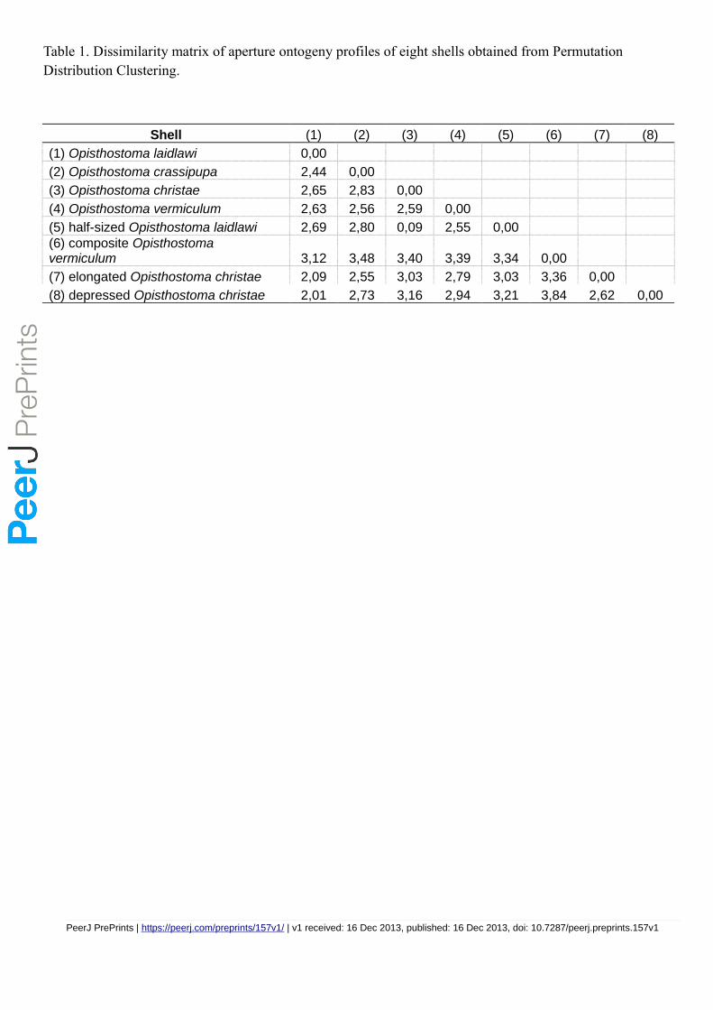
Table 1. Dissimilarity matrix of aperture ontogeny profiles of eight shells obtained from Permutation Distribution Clustering.
Shell (1) (2) (3) (4) (5) (6) (7) (8)
(1) Opisthostoma laidlawi 0,00
(2) Opisthostoma crassipupa 2,44 0,00
(3) Opisthostoma christae 2,65 2,83 0,00
(4) Opisthostoma vermiculum 2,63 2,56 2,59 0,00
(5) half-sized Opisthostoma laidlawi 2,69 2,80 0,09 2,55 0,00(6) composite Opisthostoma vermiculum 3,12 3,48 3,40 3,39 3,34 0,00
(7) elongated Opisthostoma christae 2,09 2,55 3,03 2,79 3,03 3,36 0,00
(8) depressed Opisthostoma christae 2,01 2,73 3,16 2,94 3,21 3,84 2,62 0,00
PeerJ PrePrints | https://peerj.com/preprints/157v1/ | v1 received: 16 Dec 2013, published: 16 Dec 2013, doi: 10.7287/peerj.preprints.157v1
PrePrin
ts

Figure 1
Procedures to generate a retopologised shell based on the aperture ontogeny from a
shell by using Blender software.
(A) Procedure 3 - Creating reference: Tracing aperture from shell model. (B) Procedure 3 -
Creating reference: Tracing ontogeny axis. (C) Procedure 3 – both traced aperture outline
and ontogeny axis were converted to Bezier curves. (D) Procedure 4 – Retopologising
aperture outlines from the reference by using NURBS circles in EDIT mode. (E)
Retopologised aperture outlines. (F) Procedure 4 – Generating retopologised shell surface
models from NURBS circles in EDIT mode. (G) Final retopologised NURBS surface shell
model. (H) Retopologised 3D shell mesh converted from retopologised NURBS surface shell
model.
PeerJ PrePrints | https://peerj.com/preprints/157v1/ | v1 received: 16 Dec 2013, published: 16 Dec 2013, doi: 10.7287/peerj.preprints.157v1
PrePrin
ts

PeerJ PrePrints | https://peerj.com/preprints/157v1/ | v1 received: 16 Dec 2013, published: 16 Dec 2013, doi: 10.7287/peerj.preprints.157v1
PrePrin
ts

Figure 2
Retopologised shell 3D models obtained by repotologising real shells (A – D) and by
transformation of retopologised shells (E – H).
(A) Shell of Opisthostoma laidlawi Sykes 1902. (B) Shell of Opisthostoma crassipupa van
Benthem Jutting, 1952. (C) Shell of Opisthostoma christae Maassen 2001. (D) Shell of
Opisthostoma vermiculum Clements and Vermeulen, 2008. (E) Opisthostoma laidlawi shell
that was resized by one-half and with slight modification of the last aperture size. (F)
Opisthostoma christae shell that was reshaped into an elongated form by reducing the model
size (linear dimension) by one-half along the x and y axes, and by doubling the size along the
z axis. (G) Opisthostoma christae shell that was reshaped into a depressed form by
increasing by 1.5 the model size along the x and y axes, and by reducing the size by one-half
along the z axis. (H) Opisthostoma vermiculum shell that consists of one Opisthostoma
vermiculum original 3D model of which the aperture was connected to a second, enlarged,
Opisthostoma vermiculum.
PeerJ PrePrints | https://peerj.com/preprints/157v1/ | v1 received: 16 Dec 2013, published: 16 Dec 2013, doi: 10.7287/peerj.preprints.157v1
PrePrin
ts
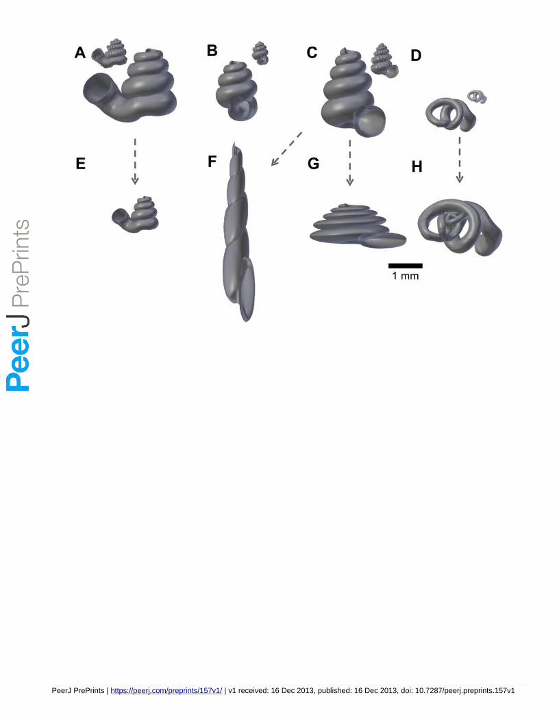
PeerJ PrePrints | https://peerj.com/preprints/157v1/ | v1 received: 16 Dec 2013, published: 16 Dec 2013, doi: 10.7287/peerj.preprints.157v1
PrePrin
ts

Figure 3
Different data types that could be obtained directly from a 3D shell model that was
retopologised on the basis of the aperture ontogeny.
(A) Aperture maps (sensu Rice, 1998) or growth vector maps (sensu Urdy et al., 2010). (B)
same as (A), but the data can be obtained in a greater resolution. (C) Aperture outlines data
for generating curve models. (D) Multiple ontogeny axes for helicospiral models. (E) Simple
3D surface shell model with no thickness. (F) 3D surface shell model with added thickness.
PeerJ PrePrints | https://peerj.com/preprints/157v1/ | v1 received: 16 Dec 2013, published: 16 Dec 2013, doi: 10.7287/peerj.preprints.157v1
PrePrin
ts

PeerJ PrePrints | https://peerj.com/preprints/157v1/ | v1 received: 16 Dec 2013, published: 16 Dec 2013, doi: 10.7287/peerj.preprints.157v1
PrePrin
ts

Figure 4
Shell size (volume) and aperture ontogeny profiles in terms of aperture growth trajectory
(curvature and torsion) and aperture form (size and shape) of eight shells.
(A) Shell of Opisthostoma laidlawi Sykes 1902. (B) Shell of Opisthostoma crassipupa van
Benthem Jutting, 1952. (C) Shell of Opisthostoma christae Maassen 2001. (D) Shell of
Opisthostoma vermiculum Clements and Vermeulen, 2008. (E) Opisthostoma laidlawi shell
that was resized by one-half and with slight modification of the last aperture size. (F)
Opisthostoma christae shell that was reshaped into an elongated form by reducing the model
size (linear dimension) by one-half along the x and y axes, and by doubling the size along the
z axis. (G) Opisthostoma christae shell that was reshaped into a depressed form by
increasing by 1.5 of the model size along the x and y axes, and by reducing the size by one-
half along the z axis. (H) Opisthostoma vermiculum shell that consists of one Opisthostoma
vermiculum original 3D model of which the aperture was connected to a second enlarged
Opisthostoma vermiculum.
PeerJ PrePrints | https://peerj.com/preprints/157v1/ | v1 received: 16 Dec 2013, published: 16 Dec 2013, doi: 10.7287/peerj.preprints.157v1
PrePrin
ts

PeerJ PrePrints | https://peerj.com/preprints/157v1/ | v1 received: 16 Dec 2013, published: 16 Dec 2013, doi: 10.7287/peerj.preprints.157v1
PrePrin
ts

Figure 5
Radar charts of the aperture ontogeny profiles of eight shells.
Each radar chart shows the value and trends of the curvature, torsion, aperture size, aperture
shape scores, and ontogeny axis length of each shell.
PeerJ PrePrints | https://peerj.com/preprints/157v1/ | v1 received: 16 Dec 2013, published: 16 Dec 2013, doi: 10.7287/peerj.preprints.157v1
PrePrin
ts

PeerJ PrePrints | https://peerj.com/preprints/157v1/ | v1 received: 16 Dec 2013, published: 16 Dec 2013, doi: 10.7287/peerj.preprints.157v1
PrePrin
ts
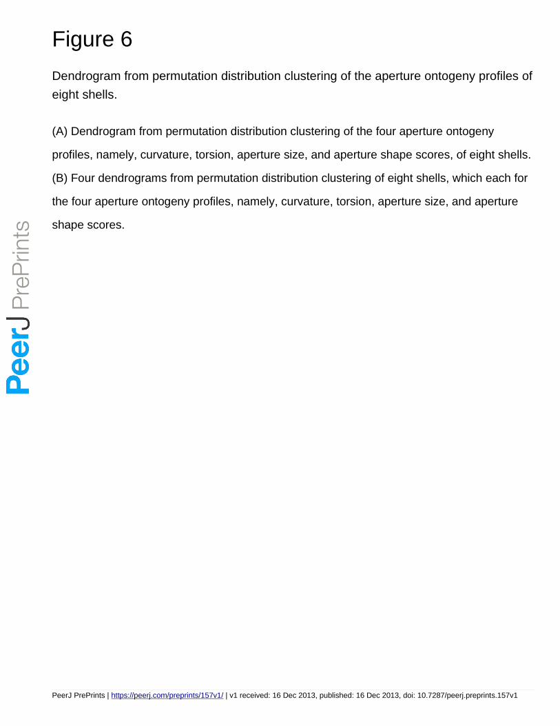
Figure 6
Dendrogram from permutation distribution clustering of the aperture ontogeny profiles of
eight shells.
(A) Dendrogram from permutation distribution clustering of the four aperture ontogeny
profiles, namely, curvature, torsion, aperture size, and aperture shape scores, of eight shells.
(B) Four dendrograms from permutation distribution clustering of eight shells, which each for
the four aperture ontogeny profiles, namely, curvature, torsion, aperture size, and aperture
shape scores.
PeerJ PrePrints | https://peerj.com/preprints/157v1/ | v1 received: 16 Dec 2013, published: 16 Dec 2013, doi: 10.7287/peerj.preprints.157v1
PrePrin
ts

PeerJ PrePrints | https://peerj.com/preprints/157v1/ | v1 received: 16 Dec 2013, published: 16 Dec 2013, doi: 10.7287/peerj.preprints.157v1
PrePrin
ts

Figure 7
Non-metric multidimensional scaling (NMDS) 3D plots as shell morphospace.
The NMDS plots were generated from a dissimilarity matrix of eight Opisthostoma shells
aperture ontogeny profiles, which were analysed by permutation distribution clustering.
PeerJ PrePrints | https://peerj.com/preprints/157v1/ | v1 received: 16 Dec 2013, published: 16 Dec 2013, doi: 10.7287/peerj.preprints.157v1
PrePrin
ts

PeerJ PrePrints | https://peerj.com/preprints/157v1/ | v1 received: 16 Dec 2013, published: 16 Dec 2013, doi: 10.7287/peerj.preprints.157v1
PrePrin
ts