Int. J. Dynam. Control (2013) 1:300–315DOI 10.1007/s40435-013-0027-8

A mean-field maximum principle for optimal controlof forward–backward stochastic differential equationswith Poisson jump processes

Mokhtar Hafayed

Received: 12 June 2013 / Revised: 2 August 2013 / Accepted: 6 August 2013 / Published online: 10 September 2013© Springer-Verlag Berlin Heidelberg 2013

Abstract We consider mean-field type stochastic opti-mal control problems for systems governed by specialmean-field forward–backward stochastic differential equa-tions with jump processes, in which the coefficients containsnot only the state process but also its marginal distribution.Moreover, the cost functional is also of mean-field type. Nec-essary conditions of optimal control for these systems in theform of a maximum principle are established by means ofspike variation techniques. Our result differs from the classi-cal one in the sense that here the adjoint equation has a mean-field type. The control domain is not assumed to be convex.

Keywords Optimal stochastic control · Mean-fieldforward–backward stochastic differential equation withjump processes · Stochastic maximum principle · Spikevariation techniques · Poisson martingale measure

Mathematics Subject Classification 93E20 · 60H10

1 Introduction

The stochastic maximum principle of optimality for systemsgoverned by forward–backward stochastic differential equa-tions (FBSDEs) has been studied by many authors, see e.g.[1–6]. The maximum principle for fully coupled forward–backward stochastic control system in global form hasbeen investigated in Shi and Wu [1]. The necessary condi-tions for partially-observed optimal control of fully-coupledforward–backward stochastic system has been studied byShi and Wu [2]. However, the necessary conditions of opti-

M. Hafayed (B)Laboratory of Applied Mathematics,Biskra University, P.O. Box 145, 07000 Biskra, Algeriae-mail: hafayedmokhtar@yahoo.com

mality for FBSDEs in global form, with uncontrolled diffu-sions coefficient was derived by Xu [3]. In a recent paper byYong [5], the author completely solved the problem of max-imum principle of optimality for fully coupled FBSDEs. Heconsidered an optimal control problem for general coupledFBSDEs with mixed initial-terminal conditions and derivedthe necessary conditions for optimality when the controlvariable appears in the diffusion coefficients of the forward-equation and the control domain is not necessarily convex. Agood account and an extensive list of references on stochas-tic maximum principle for FBSDEs with applications can befound in Ma and Yong [6].

As is well known, the stochastic optimal control problemsfor jump processes have been investigated by many authors,see e.g. [7–14]. The necessary and sufficient conditionsof optimality for forward–backward stochastic differentialequations with jump processes (FBSDEJs) was obtained byShi and Wu [7,8]. In an interesting paper, Shi [9] generalizedYong’s maximum principle for FBSDEs obtained in Yong [5]to jump case. He established the stochastic maximum prin-ciple for optimality for fully coupled FBSDEJs when thecontrol variable appears both in the diffusion and jump coef-ficients and the control domain is not assumed to be convex.

The mean-field model was initially introduced by Kac[15] as a stochastic model for the Vlasov-kinetic equationof plasma and the study of which was initiated by McKean[16]. Since then, many authors made contributions on mean-field stochastic problems with some applications, see forinstance, [17–28]. Recently, mean-field stochastic maximumprinciple of optimality was considered by many authors,see for instance [17,20,22–27]. In Lazry and Lions [23]the authors introduced a general mathematical modelingapproach for high-dimensional systems of evolution equa-tions corresponding to a large number of particles (or agents).They extended the field of such mean-field approaches also to

123

A mean-field necessary conditions for optimal stochastic control of FBSDEJs 301

problems in economics, finance and game theory. In Buck-dahn et al. [19] a general notion of mean-field backwardstochastic differential equations (BSDEs) associated with amean-field stochastic differential equation (SDE) is obtainedin a natural way as a limit of some high dimensional systemof FBSDEs governed by a d-dimensional Brownian motion,and influenced by positions of a large number of other par-ticles. In Buckdahn et al. [20] a general maximum princi-ple was introduced for a class of stochastic control prob-lems involving SDEs of mean-field type. However, the suffi-cient conditions of optimality for mean-field SDE have beenestablished by Shi [17]. In Mayer-Brandis et al. [26] a sto-chastic maximum principle of optimality for systems gov-erned by controlled Itô-Levy process of mean-field type wasproved by using Malliavin calculus. Under the conditionsthat the control domains are convex, Andersson and Dje-hiche [24] and Li [25] studied problems for two types of moregeneral controlled SDEs and cost functionals, respectively.The linear-quadratic optimal control problem for mean-fieldSDEs has been studied by Yong [27] and in Shi [17]. Themean-field stochastic maximum principle for jump diffusionprocesses has been investigated in Hafayed and Abbas [22].The macroscopic limit of stochastic partial differential equa-tions of McKean-Vlasov type has been studied by Kotelenezand Kurtz [21]. The existence result for the solution of mean-field FBSDEs has been studied by Carmona and Dularue [28].

Our goal in this paper is to establish a set of necessaryconditions of optimality for mean-field FBSDEJs, where thecoefficient depend not only on the state process but also itsmarginal law of the state process through its expected value.The cost functional is also of mean-field type. The mean-field problem under consideration is not simple extensionfrom the mathematical point of view, but also provide inter-esting models in many applications such as mathematicalfinance, optimal control for mean-field systems. The proofof our main result is based on spike variation method. Thesenecessary conditions are described in terms of two adjointprocesses, corresponding to the mean-field forward and back-ward components with jumps and a maximum conditions onthe Hamiltonian. To streamline the presentation of this paper,we only study the one dimensional case.

The plan of the rest of this paper is organized as follows.In Sect. 2 we formulate the mean-field stochastic controlproblem and describe the assumptions of the model. The lastsection is devoted to prove our stochastic maximum princi-ple for mean-field FBSDEJs which is the main result of thispaper.

2 Problem formulation and preliminaries

We consider in this paper stochastic optimal control prob-lems of mean-field type of the following kind. Let T > 0

be a fixed time horizon and (�,F , (Ft )t∈[0,T ] ,P) be a fixedfiltered probability space equipped with a P-completed rightcontinuous filtration on which a d-dimensional Brownianmotion W = (W (t))t∈[0,T ] is defined. Let η be a homo-geneous (Ft )-Poisson point process independent of W . Wedenote by ˜N (dθ, dt) the random counting measure inducedby η, defined on�× R+, where� is a fixed nonempty sub-set of R with its Borel σ -field B (�). Further, let μ (dθ) bethe local characteristic measure of η, i.e. μ (dθ) is a σ -finitemeasure on (�,B (�)) with μ (�) < +∞. We then define

N (dθ, dt) = ˜N (dθ, dt)− μ (dθ) dt,

where N (·, ·) is Poisson martingale measure on B (�) ×B (R+) with local characteristics μ (dθ) dt. We assumethat (Ft )t∈[0,T ] is P-augmentation of the natural filtration

(F (W,N )t )t∈[0,T ] defined as follows

F (W,N )t = σ (W (s) : 0 ≤ s ≤ t)

∨σ⎧

⎨

⎩

s∫

0

∫

B

N (dθ, dr), 0 ≤ s ≤ t, B ∈ B (�)⎫

⎬

⎭

∨G,where G denotes the totality of P-null sets, and σ1 ∨ σ2

denotes the σ -field generated by σ1 ∪ σ2.

In the present paper, we study stochastic optimal con-trol for a system governed by mean-field forward–backwardstochastic differential equations with jump processes (FBS-DEJs) of the form⎧

⎪

⎪

⎪

⎪

⎪

⎪

⎪

⎪

⎪

⎪

⎪

⎨

⎪

⎪

⎪

⎪

⎪

⎪

⎪

⎪

⎪

⎪

⎪

⎩

dx(t) = f (t, x(t),E(x(t)), u(t)) dt

+ σ (t, x(t),E(x(t))) dW (t)

+ ∫

�c (t, x(t−), θ) N (dθ, dt) ,

dy(t) = − ∫�

g(t, x(t),E(x(t)), y(t),E(y(t)),

z(t),E(z(t)), r (t, θ) , u(t))μ (dθ) dt

+ z(t)dW (t)+ ∫�

r (t, θ) N (dθ, dt) ,

x(0) = ζ, y(T ) = h (x(T ),E (x(T ))) ,

(1)

where f, σ, b, g, h are given maps and the initial condition ζis an F0-measurable random variable. The special mean-fieldFBSDEJs-(1), called McKean-Vlasov systems are obtainedas a limit approach, by the mean-square limit, when n →+∞ of a system of interacting particles of the form:⎧

⎪

⎪

⎪

⎪

⎪

⎪

⎪

⎪

⎪

⎪

⎪

⎪

⎪

⎨

⎪

⎪

⎪

⎪

⎪

⎪

⎪

⎪

⎪

⎪

⎪

⎪

⎪

⎩

dx jn (t) = f (t, x j

n (t),1n

∑ni=1 xi

n(t), u(t))dt

+σ(t, x jn (t),

1n

∑ni=1 xi

n(t))dW j (t)

+ ∫�

c(t, x jn (t−), θ)N j (dθ, dt) ,

dy jn (t) = − ∫

�g(t, x j

n (t),1n

∑ni=1 xi

n(t), y jn (t),

1n

∑ni=1 yi

n(t), z jn(t),

1n

∑ni=1 zi

n(t),

r(t, θ), u(t)) μ (dθ) dt

+z jn(t)dW j (t)+ ∫

�r (t, θ) N j (dθ, dt) ,

123

302 M. Hafayed

where (W j (·) : j ≥ 1) is a collection of independent Brown-ian motions and (N j (·, ·) : j ≥ 1) is a collection of inde-pendent Poisson martingale measure. Noting that mean-fieldFBSDEJs-(1) occur naturally in the probabilistic analysis offinancial optimization problems and the optimal control ofdynamics of the McKean-Vlasov type. Moreover, the abovemathematical mean-field approaches play an important rolein different fields of economics, finance, physics, chemistryand game theory.

The expected cost on the time interval [0, T ] is defined by

J (u(·)) = E [ϕ (y(0),E (y(0)))] . (2)

This cost functional is also of mean-field type, as the functionϕ depends on the marginal law of the state process through itsexpected value, which makes the control problem time incon-sistent in the sense that the dynamic programming principlefor optimality does not hold.

An admissible control u(·) is an Ft -adapted and square-integrable process with values in a nonempty subset A of R.

We denote the set of all admissible controls by U ([0, T ]).Any admissible control u∗(·) ∈ U ([0, T ]) satisfying

J(

u∗(·)) = infu(·)∈U([0,T ])

J (u(·)) , (3)

is called an optimal control.The corresponding state process, solution of FBSDEJ-(1),

is denoted by (x∗(·), y∗(·), z∗(·), r∗(·, ·)) .

2.1 Notations

For convenience, we will use the following notations in thispaper

1. In the sequel, L2F ([0, T ] ; R) denotes the Hilbert space of

Ft -adapted processes ((t))t∈[0,T ] such that E∫ t

0 |(t)|2dt < +∞.

2. M2F ([0, T ] ; R) denotes the Hilbert space of Ft -predic-

table processes (ψ (t, θ))t∈[0,T ] defined on [0, T ] ×� × � such that E

∫ T0

∫

�|ψ (t, θ)|2 μ(θ)dt < +∞.

3. We denote by IA the indicator function of A and (x, y, z)denotes the expected value of (x, y, z).

4. For a differentiable function � we denote by �ρ(t) itsgradient with respect to the variable ρ.

5. For convenience, we will use the following

δ f (t) = f(

t, x∗(t),E(x∗(t)), u(t))

− f(

t, x∗(t),E(x∗(t)), u∗(t))

,

and

δg(t, θ) = g(t, x∗(t),E(x∗(t)), y∗(t),E(y∗(t)),z∗(t),E(z∗(t)), r∗(t, θ), u(t))

−g(t, x∗(t),E(x∗(t)), y∗(t),E(y∗(t)),z∗(t),E(z∗(t)), r∗(t, θ), u∗(t)).

6. In what follows, C represents a generic constant, whichcan be different from line to line.

2.2 Conditions

Throughout this paper, we also assume that the coefficientsfunctions

f : [0, T ] × R × R × A → R,

σ : [0, T ] × R × R → R,

c : [0, T ] × R×� → R,

g : [0, T ] × R × R × R × R × R × R × R × A → R,

h : R × R → R,

ϕ : R → R,

satisfy the following standing assumptions

2.2.1 Condition (H1)

The functions f, σ, b, g, h, ϕ are continuously differentiablewith respect to (x, x, y, y, z, z, r).

2.2.2 Condition (H2)

The derivatives of f, σ, b, h, ϕ with respect to (x, x, y, y, z,z, r) are bounded and there is a constant C > 0 such thatsupθ∈� |g(t, θ)| < C for = x, x, y, y, z, z, r.

Under the assumptions (H1) and (H2), the FBSDEJ-(1)has an unique solution (x(t), y(t), z(t), r(t, ·)) ∈ L

2F ([0, T ];

R)× L2F ([0, T ] ; R)× L

2F ([0, T ] ; R)× L

2F ([0, T ] ; R).

For any u(·) ∈ U ([0, T ]) with its corresponding statetrajectories (x (·) , y (·) , z (·) , r(·, ·)) we introduce the fol-lowing adjoint equations

⎧

⎪

⎪

⎪

⎪

⎪

⎪

⎪

⎪

⎪

⎪

⎪

⎪

⎪

⎪

⎪

⎪

⎪

⎪

⎪

⎪

⎪

⎨

⎪

⎪

⎪

⎪

⎪

⎪

⎪

⎪

⎪

⎪

⎪

⎪

⎪

⎪

⎪

⎪

⎪

⎪

⎪

⎪

⎪

⎩

d�(t) = −{ fx (t)�(t)+ E [ fx (t)�(t)]

+σx (t) Q(t)+ E [σx (t) Q(t)]

+ ∫�

[

gx (t, θ)K (t)+ E (gx (t, θ)K (t))

+ cx (t, θ) Rt (θ)]μ (dθ)}dt

+Q(t)dW (t)+ ∫�

Rt (θ) N (dθ, dt) ,

�(T ) = −{hx (T ) K (T )+ E [(hx (T )) K (T )]} .d K (t) = ∫

�

[

gy (t, θ) K (t)+ E(

gy (t, θ) K (t))]

μ (dθ) dt

+ ∫�

[

gz(t, θ)K (t)+ E (gz(t, θ)K (t))]

μ (dθ) dW (t)

− ∫�

gr (t, θ)K (t)N (dθ, dt)

K (0) = − {ϕy (y(0),E (y(0)))

+ E[

ϕy (y(0),E (y(0)))]}

,

(4)

123

A mean-field necessary conditions for optimal stochastic control of FBSDEJs 303

where

fρ(t) = ∂ f

∂ρ(t, x(t),E(x(t)), u(t)) , for ρ = x, x,

σρ (t) = ∂σ

∂ρ(t, x(t),E(x(t))) , for ρ = x, x,

cx (t, θ) = cx (t, x, θ),

hρ (t) = ∂h

∂ρ(x(t),E(x(t))) , for ρ = x, x,

ϕρ (t) = ∂ϕ

∂ρ(y(t),E(y(t))) , for ρ = y, y,

gρ(t, θ)= ∂g

∂ρ(t, x(t),E(x(t)), y(t),E(y(t)), z(t),E(z(t)),

r(t, θ), u(t)), for ρ = x, x, y, y, z, z, r.

Note that the first adjoint equation (backward) correspond-ing to the forward component x(·) turns out to be a linearmean-field backward SDE with jumps, and the second adjointequation (forward) corresponding to the backward compo-nent (y(·), z(·), r(·, ·)) turns out to be a linear mean-field(forward) SDE with jump processes.

Further, we define the Hamiltonian function

H : [0, T ] × R × R × R × R × R × R × R

×A × R × R × R × R → R,

associated with the stochastic control problem (1)–(2) as fol-lows

H (t, x, x, y, y, z, z, r(·), u, �, Q, K , R(·))= �(t) f (t, x, x, u)+ Q(t)σ (t, x, x)

+∫

�

[K (t)g (t, x, x, y, y, z, z, r(t, θ), u)

+ R (t, θ) c (t, x, θ))]μ (dθ) . (5)

If we denote by

H (t) = H(t, x(t), x(t), y(t), y(t), z(t), z(t),

r(t, ·), u(t),�(t), Q(t), K (t), Rt (·)),then the adjoint equation (4) can be rewritten as the followingstochastic Hamiltonian system’s type⎧

⎪

⎪

⎪

⎪

⎪

⎪

⎪

⎪

⎪

⎪

⎪

⎪

⎪

⎪

⎪

⎪

⎨

⎪

⎪

⎪

⎪

⎪

⎪

⎪

⎪

⎪

⎪

⎪

⎪

⎪

⎪

⎪

⎪

⎩

d�(t) = −{Hx (t)+ E [Hx (t)]} dt

+ Q(t)dW (t)+ ∫�

Rt (θ) N (dθ, dt) ,

�(T ) = − [hx (T )+ E (hx (T ))] K (T )

− d K (t) = [Hy (t)+ E(

Hy (t))]

dt

+ [Hz (t)+ E (Hz (t))]

dW (t)

+ ∫�

Hr (t−, θ) N (dθ, dt)

K (0) = − {ϕy (y(0),E (y(0)))

+ E[

ϕy (y(0),E (y(0)))]}

.

(6)

It is a well known fact that under assumptions (H1) and(H2), the adjoint equation (4) admits a unique solution

(�(t), Q(t), K (t), R(t, ·)) such that

(�(t), Q(t), K (t), Rt (·)) ∈ L2F ([0, T ] ; R)

× L2F ([0, T ] ; R)× L

2F ([0, T ] ; R)× M

2F ([0, T ] ; R).

Moreover, since the derivatives of fx , fx , σx , σx , cx , gx , gx ,

gy, gy, gz, gz, gr , hx , hx , ϕy and ϕy are bounded, we deducefrom standard arguments that there exists a constant C > 0such that

E

⎡

⎣ supt∈[0,T ]

|�(t)|2 + supt∈[0,T ]

|K (t)|2 dt

+T∫

0

|Q(t)|2 dt +T∫

0

∫

�

|Rt (θ)|2 μ (dθ) dt

⎤

⎦ < C. (7)

3 Mean-field type maximum principle for FBSDEJs

In this section, we establish a set of necessary conditionsof Pontraygin’s type for a stochastic control to be optimalwhere the system evolves according to nonlinear controlledmean-field FBSDEJs. Spike variation techniques are appliedto prove our mean-field stochastic maximum principle.

The following theorem constitutes the main contributionof this paper.

Let (x∗(·), y∗(·), z∗(·), r∗(·, ·)) be the trajectory of themean-field FBSDEJ-(1) corresponding to the optimal con-trol u∗(·), and (�∗(·), Q∗(·), K ∗(·), R∗(·)) be the solutionof adjoint equation (4) corresponding to u∗(·).Theorem 3.1 Let Assumptions (H1) and (H2) hold. If(u∗(·), x∗(·), y∗(·), z∗(·), r∗(·, ·)) is an optimal solution ofthe mean-field control problem (1 )–( 2 ). Then the maximumprinciple holds, that is

H(t, λ∗(t, θ), u∗(t),�∗(t, θ))= minu∈A, H(t, λ∗(t, θ), u,�∗(t, θ))

P − a.s., a.e. t ∈ [0, T ] , (8)

where

λ∗(t, θ) = (x∗(t),E(x∗(t)), y∗(t),E(y∗(t)), z∗(t),E(z∗(t)), r∗(t, θ))

�∗(t, θ) = (�∗(t), Q∗(t), K ∗(t), R∗(t, θ)).

To prove Theorem 3.1 we need some preliminary resultsgiven in the following Lemmas. We derive the variationalinequality (8) in several steps, from the fact that

J(

uε(·)) ≥ J(

u∗(·)) , (9)

where uε(·) is the so called spike variation of optimal controlu∗(·) defined as follows.

123

304 M. Hafayed

For ε > 0, we choose a Borel measurable set Aε ⊂ [0, T ]such that ν(Aε) = ε, where ν(Aε) denote the Lebesguemeasure of the subsetAε, and we consider the control processwhich is the spike variation of u∗(·)

uε(t) ={

u : t ∈ Aε,

u∗(t) : t ∈ Acε,

where ε > 0 is sufficiently small and u is an arbitrary elementFt -measurable random variable with values in A, such thatsupw∈� |u(w)| < ∞, which we consider as fixed from nowon.

Let λε(·) = (xε(·), yε(·), zε(·), rε(·, ·)) be the solution ofFBSDEJs-(1) and �ε(·) = (�ε (·) , Qε (·) , K ε (·) , Rε (·))be the solution of the adjoint equation (4) corresponding touε(·).

3.1 Variational equations

Now, we introduce the following variational equations. Forsimplicity of notation, we will still use δ�(t) where u(t) =uε(t), for � = f, g, etc. and fx (t) = ∂ f

∂x(t, x∗,E(x∗), u∗),

etc. Let(

xε1(·), yε1(·), zε1(·), rε1 (·, ·))

be the solution of thefollowing mean-field forward backward stochastic system⎧

⎪

⎪

⎪

⎪

⎪

⎪

⎪

⎪

⎪

⎪

⎪

⎪

⎪

⎪

⎪

⎪

⎪

⎨

⎪

⎪

⎪

⎪

⎪

⎪

⎪

⎪

⎪

⎪

⎪

⎪

⎪

⎪

⎪

⎪

⎪

⎩

dxε1(t) = { fx (t)xε1(t)+ fx (t)E(

xε1(t))

+ δ f (t)IAε(t)}

dt+ {σx (t)xε1(t)+ σx (t)E

(

xε1(t))}

dW (t)+ ∫

�cx (t, θ)xε1(t)N (dθ, dt),

xε1(0) = 0,dyε1(t) = ∫

�

{

gx (t, θ)xε1(t)+ gx (t, θ)E(xε1(t))+ gy(t, θ)yε1(t)+ gy(t, θ)E(yε1(t))+ gz(t, θ)zε1(t)+ gz(t, θ)E(zε1(t))+ gr (t, θ)rε1 (t, θ)+ δg(t, θ)IAε

(t)}

μ(dθ)dt+ zε1(t)dW (t)− ∫

�rε1 (t, θ)N (dθ, dt)

yε1(T ) = − [hx (T )+ E (hx (T )))] xε1(T ).

(10)

Noting that the variational equations (10) is also a FBSDEJsof mean-field type.

3.2 Duality

Our first Lemma below deals with the duality relationsbetween �∗(t), xε1(t) and K ∗(t), yε1(t).

Lemma 3.1 We have

E(

�∗(T )xε1(T )) = E

T∫

0

�∗(t)δ f (t)IAε(t)dt

− E

T∫

0

∫

�

xε1(t)[

E(

gx (t, θ)K∗(t))

+ gx (t, θ) K ∗(t)]

μ(dθ)dt, (11)

E(

K ∗(T )yε1(T )) = − E

{

ϕy (y(0),E (y(0)))

+ E(

ϕy (y(0),E (y(0))))

)yε1(0)}

+E

T∫

0

∫

�

{

K ∗(t)gx (t, θ)xε1(t)

+K ∗(t)gx (t, θ)E(

xε1(t))

+ K ∗(t)δg(t, θ)IAε(t)}

μ(dθ)dt,

(12)

and

E{[

ϕy (y(0),E (y(0)))+ E(

ϕy (y(0),E (y(0))))]

yε1(0)}

= E

T∫

0

⎡

⎣�∗ (t) δ f (t)+∫

�

K ∗ (t) δg(t, θ)μ(dθ)IAε(t)

⎤

⎦ dt.

(13)

Proof This Lemma is very important for the proof of ourresult. So that we give its detailed proof. By applying inte-gration by parts formula for jump processes (see Lemma A1)to �∗(t)xε1(t), we get

E(

�∗(T )xε1(T )) = E

T∫

0

�∗(t)dxε1(t)+ E

T∫

0

xε1(t)d�∗(t)

+ E

T∫

0

Q∗(t)[

σx (t)xε1(t)+ σx (t)E

(

xε1(t))]

dt

+ E

T∫

0

∫

�

cx (t, θ)xε1(t)Rt (θ)μ(dθ)dt

= I ε1 + I ε2 + I ε3 + I ε4 . (14)

A simple computation shows that

I ε1 = E

T∫

0

�∗(t)dxε1(t)

= E

T∫

0

{

�∗(t) fx (t)xε1(t)+�∗(t) fx (t)E

(

xε1(t))

+ �∗(t)δ f (t)IAε(t)}

dt, (15)

and

I ε2 = E

T∫

0

xε1(t)d�∗(t)

= −E

T∫

0

{

xε1(t) fx (t)�∗(t)+ xε1(t)E

(

fx (t)�∗(t))

+xε1(t)σx (t) Q∗(t)+ xε1(t)E(

σx (t)Q∗(t))

123

A mean-field necessary conditions for optimal stochastic control of FBSDEJs 305

+∫

�

(xε1(t)gx (t, θ) K ∗(t)+ xε1(t)E(

gx (t, θ)K∗(t))

+ cx (t, θ) Rt (θ))μ (dθ)} dt. (16)

By standard arguments we get

I ε3 = E

T∫

0

Q∗(t)σx (t)xε1(t)dt

+ E

T∫

0

Q∗(t)σx (t)E(

xε1(t))

dt

I ε4 = E

T∫

0

∫

�

cx (t, θ)xε1(t)Rt (θ)μ(dθ)dt. (17)

The duality relation (11) follows immediately from combin-ing (15)–(17) and (14).

Let us turn to second duality relation (12). By applyingintegration by parts formula for jump process (Lemma A1)to K ∗(t)yε1(t) we get

E(

K ∗(T )yε1(T )) = E

(

K ∗(0)yε1(0))

+ E

T∫

0

K ∗(t)dyε1(t)+ E

T∫

0

yε1(t)d K ∗(t)

− E

T∫

0

zε1(t)[

gz(t)K∗(t)+ E

(

gz(t)K∗(t))]

dt

− E

T∫

0

∫

�

rε1 (t, θ)gr (t, θ)K (t)μ(dθ)dt.

= I ε1 + I ε2 + I ε3 + I ε4 + I ε5 . (18)

From (10) we obtain

I ε2 = E

T∫

0

K ∗(t)dyε1(t)

= E

T∫

0

∫

�

{

K ∗(t)gx (t, θ)xε1(t)

+ K ∗(t)gx (t, θ)E(

xε1(t))

+ K ∗(t)gy(t, θ)yε1(t)+ K ∗(t)gy(t, θ)E

(

yε1(t))

+ K ∗(t)gz(t, θ)zε1(t)+ K ∗(t)gz(t, θ)E

(

zε1(t))

+ K ∗(t)gr (t, θ)rε1 (t, θ)

+ K ∗(t)δg(t, θ)IAε(t)}

μ(dθ)dt, (19)

from (4), we obtain

I ε3 = E

T∫

0

yε1(t)d K ∗(t)

= −E

T∫

0

∫

�

{

yε1(t)gy (t, θ) K ∗(t)

+ yε1(t)E(

gy(t, θ)K∗(t))}

μ(dθ)dt, (20)

and

I ε4 = −E

T∫

0

∫

�

[

zε1(t)gz(t, θ)K∗(t)

+ zε1(t)E(

gz(t, θ)K∗(t))]

μ(dθ)dt

I ε5 = −E

T∫

0

∫

�

rε1 (t, θ)gr (t, θ)K∗(t)μ(dθ)dt. (21)

Since

I ε1 = E(

K ∗(0)yε1(0))

= −E{[ϕy (y(0),E (y(0)))

+ E(

ϕy (y(0),E (y(0))))]yε1(0)

}

,

the duality relation (12) follows immediately by combining(19)–(21) and (18).

Let us turn to (13). From (4) and (11) we deduce

E(

�∗(T )xε1(T ))+ E

(

K ∗(T )yε1(T )) = 0.

Combining (11) and (12), then (13) follows immediately. ��To this end we give the following estimations.

3.3 Some prior estimates

Lemma 3.2 Under Assumptions (H1) and (H2), the follow-ing estimations holds: for any k ≥ 1

E(sup0≤t≤T

∣

∣xε1(t)∣

∣

2k) ≤ Ckε

k,

E(sup0≤t≤T

∣

∣yε1(t)∣

∣

2)

+ E

T∫

0

⎡

⎣

∣

∣zε1(s)∣

∣

2 +∫

�

∣

∣rε1 (s, θ)∣

∣

2μ(dθ)

⎤

⎦ ds ≤ Cε2,

(22)

sup0≤t≤T

∣

∣E(

xε1(t))∣

∣

2 ≤ Cε2,

sup0≤t≤T

∣

∣E(

yε1(t))∣

∣

2 +T∫

t

∣

∣E(

zε1(s))∣

∣

2ds

+T∫

0

∫

�

∣

∣E(

rε1 (s, θ))∣

∣

2μ(dθ)ds ≤ C ρ(ε). (23)

123

306 M. Hafayed

E(sup0≤t≤T

∣

∣xε(t)− x∗(t)∣

∣

2k) ≤ Ckε

k,

E(sup0≤t≤T

∣

∣yε(t)− y∗(t)∣

∣

2) ≤ Cε2,

E

T∫

t

∣

∣zε(s)− z∗(s)∣

∣

2ds ≤ Cε2,

E

T∫

0

∫

�

∣

∣rε(s, θ)− r∗(s, θ)∣

∣

2μ(dθ)ds ≤ Cε2, (24)

and

E(sup0≤t≤T

∣

∣xε(t)− x∗(t)− xε1(t)∣

∣

2k) ≤ Ckε

2k .

E(sup0≤t≤T

∣

∣yε(t)− y∗(t)− yε1(t)∣

∣

2k) ≤ Ckε

2k .

E

T∫

t

∣

∣zε(s)− z∗(s)− zε1(s)∣

∣

2ds ≤ Cε2,

E

T∫

t

∫

�

∣

∣rε(s, θ)− r∗(s, θ)− rε1 (s, θ)∣

∣

2μ(dθ)ds ≤ Cε2,

(25)

where Ck is a positive constant depend to k and ρ(ε) → 0as ε → 0.

Noting that estimate (24) follows from standard arguments(see Shi [7], Lemma 2.1). Estimate (23) will be derived as aconsequence of the following Lemma.

Lemma 3.3 For any progressively measurable processes(� (s))s∈[0,T ] , (ψ (s))s∈[t,T ] and (φ (s, θ))(s,θ)∈[t,T ]×� forany p ≥ 1, there exists a positive constants C and C p suchthat

E(sup0≤t≤T |�(t)|p) ≤ C p,

E

T∫

t

|ψ(s)|2 ds ≤ C,

E

T∫

t

∫

�

|φ (s, θ)|2 μ(dθ)ds ≤ C, (26)

then we have for ε > 0

∣

∣E(

xε1(T )�(T ))∣

∣

2+T∫

0

∣

∣E(

xε1(t)�(t))∣

∣

2dt ≤C ρ (ε) , (27)

and

∣

∣E(

yε1(T )�(T ))∣

∣

2 +T∫

0

∣

∣E(

yε1(s)�(s))∣

∣

2ds ≤ C ρ (ε),

∣

∣E(

zε1 (T ) ψ (T ))∣

∣

2 +∫

�

∣

∣E(

rε1 (T, θ) φ (T, θ))∣

∣

2μ(dθ)

+T∫

t

⎧

⎨

⎩

∣

∣E(

zε1 (s) ψ (s))∣

∣

2

+∫

�

∣

∣E(

rε1 (s, θ) φ (s, θ))∣

∣

2μ(dθ)

⎫

⎬

⎭

ds

≤ C(T,μ(�))ρ (ε) , (28)

where ρ (ε) = (ε + ε2)→ 0, ε → 0.

Proof of estimate (27) First we set for t ∈ [0, T ] : η (t) =exp {M(t)} , where

M (t) = −t∫

0

⎡

⎣fx (s)− 1

2|σx (s)|2 − 1

2

∫

�

(cx (s, θ))2 μ(dθ)

⎤

⎦ ds

−t∫

0

σx (s)dW (s)−t∫

0

∫

�

cx (s−, θ)N (dθ, ds),

and we denote by ρ (t) = η (t)−1 = exp {−M(t)} .By using Itô formula for exp {M(t)} , we get

d (exp {M(t)}) = exp {M(t)} d M(t)

+1

2exp {M(t)} d 〈M(t); M(t)〉 ,

this shows that

dη (t) = d (exp {M(t)})

= −η (t)⎧

⎨

⎩

⎡

⎣fx (t)− (σx (t))2 −

∫

�

(cx (t, θ))2 μ(dθ)

⎤

⎦ dt

+ σx (t)dW (t)+∫

�

cx (t−, θ)N (dθ, dt)

⎫

⎬

⎭

. (29)

By using Integration by parts formula for jumps processesη (t) xε1(t) we have

d(

η (t) xε1(t)) = η (t) dxε1(t)+ xε1(t)dη (t)

+ d⟨

η (t) , xε1(t)⟩

,

= I ε1 + I ε2 + I ε3 .

From (10) we get

I ε1 = η (t) dxε1(t)

= η (t)

⎧

⎨

⎩

[

fx (t)xε1(t)+ fx (t)E

(

xε1(t))

+ δ f (t)IAε(t)]

dt

+ [σx (t)xε1(t)+ σx (t)E

(

xε1(t))]

dW (t)

+∫

�

cx (t−, θ) xε1(t)N (dθ, dt)

⎫

⎬

⎭

.

123

A mean-field necessary conditions for optimal stochastic control of FBSDEJs 307

By using (29) we get

I ε2 = xε1(t)dη (t)

= −η (t) fx (t)xε1(t)dt − η (t) σx (t)x

ε1(t)dW (t)

−η (t) xε1(t)∫

�

cx (t−, θ)N (dθ, dt)

+ η (t) xε1(t) (σx (t))2 dt

+ η (t)∫

�

(cx (t−, θ))2 xε1(t)μ(dθ)dt,

and by a simple computation we get

I ε3 = d⟨

η (t) , xε1(t)⟩

= −η (t) σx (t)[

σx (t)xε1(t)+ σx (t)E

(

xε1(t))]

dt

−∫

�

η (t) (cx (t, θ))2 xε1(t)μ(dθ)dt.

Consequently, from the above equations we deduce that

d(

η (t) xε1(t)) = I ε1 + I ε2 + I ε3

= η (t){

( fx (t)E(

xε1(t))+ δ f (t)IAε

(t)

− σx (t)σx (t)E(

xε1(t))

)dt

+ σx (t)E(

xε1(t))

dW (t)}

,

by integrating the above equation and the fact ρ (t) = η (t)−1

we obtain

xε1(t) = ρ (t)

t∫

0

η (s)× {[ fx (s)E(

xε1(s))+ δ f (t)IAε

(s)]

− σx (s)σx (s)E(

xε1(s))}

ds

+ρ (t)t∫

0

η (s) σx (s)E(

xε1(s))

dW (s). (30)

From (30) and the fact that fx , σx , cx (·, θ) are bounded, thenby using Proposition A1, we get

for all p > 1 there exists a positive constant C =C(T,p,μ(�)) such that

E

⎡

⎣ sup0≤t≤T

∣

∣

∣

∣

∣

∣

t∫

0

∫

�

cx (s−, θ) N (dθ, ds)

∣

∣

∣

∣

∣

∣

p⎤

⎦

≤ C(T,p,μ(�))E

⎡

⎣

T∫

0

∫

�

|cx (s, θ)|p μ(dθ)ds

⎤

⎦,

which shows that for all p > 1

E

[

sup0≤t≤T

(|η (t)|p + |ρ (t)|p)

]

≤ C(T,p,μ(�)). (31)

Moreover, it follows from (26) that for all p > 1

E

[

sup0≤t≤T

|�(t) ρ (t)|p)

]

≤ C(T,p,μ(�)). (32)

Next, since Ft = (F (W,N )t )t∈[s,T ] then by applying Mar-

tingale Representation Theorem for Jump Processes (seeLemma A2), there exists a unique processγt (·) ∈ L

2F ([0, t])

and unique ξt (·, θ) ∈ M2F ([0, t]) such that ∀t ∈ [0, T ] :

�(t) ρ (t) = E (� (t) ρ (t))+t∫

0

γt (s) dW (s)

+t∫

0

∫

�

ξt (s, θ)N (dθ, ds). P − a.s. (33)

Noting that, for every p > 1, with the help of (30) it followsfrom the Burkholder–Davis–Gundy inequality and Proposi-tion A1 that there exists a constant C(T,p,μ(�)) such that forp > 1,

E

⎡

⎢

⎣

⎛

⎝

t∫

0

|γt (s)|2 ds

⎞

⎠

p2⎤

⎥

⎦

+ E

⎡

⎢

⎣

⎛

⎝

t∫

0

∫

�

|ξt (s, θ)|2 μ(dθ)ds

⎞

⎠

p2⎤

⎥

⎦

≤ C pE

⎡

⎣sup0≤τ≤t

∣

∣

∣

∣

∣

∣

τ∫

0

γt (s) dW (s)

∣

∣

∣

∣

∣

∣

p⎤

⎦

+ C(T,p,μ(�))E

⎡

⎣sup0≤τ≤t

∣

∣

∣

∣

∣

∣

τ∫

0

∫

�

ξt (s−, θ)N (dθ, ds)

∣

∣

∣

∣

∣

∣

p⎤

⎦

≤ C p

(

1 + 1p−1

)pE

⎡

⎣

∣

∣

∣

∣

∣

∣

t∫

0

γt (s) dW (s)

∣

∣

∣

∣

∣

∣

p⎤

⎦

+ C(T,p,μ(�))E

⎡

⎣

∣

∣

∣

∣

∣

∣

t∫

0

∫

�

ξt (s−, θ)N (dθ, ds)

∣

∣

∣

∣

∣

∣

p⎤

⎦

≤ C(T,p,μ(�))E[|�(t) ρ (t)− E (� (t) ρ (t))|p]

≤ C(T,p,μ(�)){

E(|�(t) ρ (t)|p)+ |E (� (t) ρ (t))|p}

≤ C(T,p,μ(�))E[|�(t) ρ (t)|p]

≤ C(T,p,μ(�))E[

sup0≤t≤T |�(t) ρ (t)|p] ≤ C(T,p,μ(�))

This implies that

sup0≤t≤T

E

⎡

⎢

⎣

⎛

⎝

t∫

0

|γt (r)|2 dr

⎞

⎠

p2⎤

⎥

⎦≤ C(T,p,μ(�)), (34)

and

sup0≤t≤T

E

⎡

⎢

⎣

⎛

⎝

t∫

0

∫

�

|ξt (s, θ)|2 μ(dθ)ds

⎞

⎠

p2⎤

⎥

⎦≤ C(T,p,μ(�)).

(35)

123

308 M. Hafayed

Now, we consider

�(t) xε1 (t) = J ε1 (t)+ J ε

2 (t), t ∈ [0, T ] , (36)

where

J ε1 (t) = �(t) ρ (t)

×t∫

0

η (s){[

fx (s)E(

xε1(s))+ δ f (t)IAε

(s)]

− σx (s)σx (s)E(

xε1(s))}

ds,

and

J ε2 (t) = �(t) ρ (t)

t∫

0

η (s) σx (s)E(

xε1(s))

dW (s).

We estimate the first term in the right-hand side of (36). Sincefx , σx and σx are bounded we get∣

∣E(J ε

1 (t))∣

∣

=∣

∣

∣

∣

∣

∣

E

⎧

⎨

⎩

�(t) ρ (t)

t∫

0

η (s)[

( fx (s)− σx (s)σx (s))E(

xε1(s))

+δ f (t)IAε(s)]

ds

⎫

⎬

⎭

∣

∣

∣

∣

∣

∣

≤ C(μ(�))E

⎧

⎨

⎩

supt∈[0,T ] |�(t) ρ (t)| supt∈[0,T ] |η (t)|

×⎡

⎣

t∫

0

∣

∣E(

xε1(s))∣

∣ ds + ε

⎤

⎦

⎫

⎬

⎭

,

applying Cauchy–Schwarz inequality, then from (31) and(32) (with p = 2), we get∣

∣E(J ε

1 (t))∣

∣

≤ C(μ(�))[

E

(

supt∈[0,T ] |�(t) ρ (t)|2)] 1

2

×[

E

(

supt∈[0,T ] |η (t)|2)] 1

2

⎡

⎣

t∫

0

∣

∣E(

xε1(s))∣

∣ ds + ε

⎤

⎦

≤ C(T,μ(�))

⎡

⎣

t∫

0

∣

∣E(

xε1(s))∣

∣ ds + ε

⎤

⎦,

by applying Cauchy–Schwarz inequality and the fact that(α + β)2 ≤ 2α2 + 2β2 we can shows that∣

∣E(J ε

1 (t))∣

∣

2

≤ C(T,μ(�))

⎡

⎢

⎣

⎛

⎝

t∫

0

∣

∣E(

xε1(s))∣

∣ ds

⎞

⎠

2

+ ε2

⎤

⎥

⎦

≤ C(T,μ(�))

⎡

⎣

t∫

0

∣

∣E(

xε1(s))∣

∣

2ds + ε2

⎤

⎦. (37)

Next, we proceed to estimate the second term J ε2 (t). With

the help of (33) and the Itô Isometry we have

E(J ε

2 (t)) = E

⎧

⎨

⎩

�(t) ρ (t)

t∫

0

η (s) σx (s)E(

xε1(s))

dW (s)

⎫

⎬

⎭

= E

⎧

⎨

⎩

⎡

⎣E (� (t) ρ (t))+t∫

0

γt (s) dW (s)

+t∫

0

∫

�

ξt (s−, θ)N (dθ, ds)

⎤

⎦

×t∫

0

η (s) σx (s)E(

xε1(s))

dW (s)

⎫

⎬

⎭

= E

⎡

⎣

t∫

0

γt (s) η (s) σx (s)E(

xε1(s))

ds

⎤

⎦.

Applying (31)–(34) we obtain

E(J ε

2 (t)) ≤

∣

∣

∣

∣

∣

∣

E

t∫

0

γt (s) η (s) σx (s)E(

xε1(s))

ds

∣

∣

∣

∣

∣

∣

2

≤ C

t∫

0

∣

∣E(

xε1(s))∣

∣

2ds. (38)

By combining (35)–(38) and the fact that∣

∣E(

�(t) xε1 (t))∣

∣

2 ≤ 2∣

∣E(J ε

1 (t))∣

∣

2 + 2∣

∣E(J ε

2 (t))∣

∣

2, t ∈ [0, T ] ,

(39)

we conclude∣

∣E(

�(t) xε1 (t))∣

∣

2

≤ C(T,μ(�))

⎡

⎣ε2 + ε +t∫

0

∣

∣E(

xε1 (s))∣

∣

2ds

⎤

⎦, (40)

integrating the above inequality, we get

t∫

0

∣

∣E(

�(s) xε1 (s))∣

∣

2ds

≤ C(T,μ(�))

⎡

⎣ε2 + ε +t∫

0

r∫

0

∣

∣E(

xε1 (s))∣

∣

2dsdr

⎤

⎦. (41)

Now, taking �(t) = 1 in (41) and from Gronwall’s Lemmawe have

t∫

0

∣

∣E(

xε1 (s))∣

∣

2ds ≤ C(T,μ(�))

(

ε2 + ε)

. (42)

123

A mean-field necessary conditions for optimal stochastic control of FBSDEJs 309

Consequently, from (41) it holds that

t∫

0

∣

∣E(

�(s) xε1 (s))∣

∣

2ds ≤ C(T,μ(�))

(

ε2 + ε)

. (43)

By combining (40), and (42) we conclude

∣

∣E(

�(T ) xε1 (T ))∣

∣

2 ≤ C(T,μ(�))(

ε2 + ε)

. (44)

Finally, by setting ρ (ε) = (

ε + ε2) → 0, ε → 0, then the

desired result (27) follows immediately from (43) and (44)��

Proof of estimate (28) Applying similar argument devel-oped above we can shows that

t∫

0

∣

∣E(

yε1 (s)� (s))∣

∣

2ds ≤ C(T,μ(�))ρ (ε) and

∣

∣E(

�(T ) yε1 (T ))∣

∣

2 ≤ C(T,μ(�))ρ (ε) ,T∫

t

⎧

⎨

⎩

∣

∣E(

zε1 (s) ψ (s))∣

∣

2+∫

�

∣

∣E(

rε1 (s, θ) φ (s, θ))∣

∣

2μ(dθ)

⎫

⎬

⎭

ds

≤ C(T,μ(�))ρ (ε) ,

and for t ∈ [T − τ, T ] .

∣

∣E(

zε1 (T ) ψ (T ))∣

∣

2 +∫

�

∣

∣E(

rε1 (T, θ) φ (T, θ))∣

∣

2μ(dθ)

≤ C(T,μ(�))ρ (ε).

Finally, by using similar iterative method (see Xu [3] andalso proof of (22)) then after finite number of iterationsthe desired result (28) follows. This completes the proof ofLemma 3.3. ��

Proof of estimate (22) The first estimate can be proved bystandard arguments. By squaring both sides of

−yε1(t)−T∫

t

zε1(s)dW (s)+T∫

t

∫

�

rε1 (s, θ)N (dθ, ds)

= − [hx (T )+ E (hx (T )))] xε1(T )

+T∫

t

∫

�

{

gx (s, θ)xε1(s)+ gx (s, θ)E(x

ε1(s))

+ gy(s, θ)yε1(s)+ gy(s, θ)E(y

ε1(s))

+ gz(s, θ)zε1(s)+ gz(s, θ)E(z

ε1(s))

+ gr (t, θ)rε1 (t, θ)+ δg(t, θ)IAε

(t)}

μ(dθ)ds,

and the fact that

E

⎡

⎣yε1(t)

T∫

t

zε1(s)dW (s)

⎤

⎦ = 0,

E

⎡

⎣yε1(t)

T∫

t

∫

�

rε1 (s, θ)N (dθ, ds)

⎤

⎦ = 0,

E

⎡

⎣

T∫

t

zε1(s)dW (s)

T∫

t

∫

�

rε1 (s, θ)N (dθ, ds)

⎤

⎦ = 0,

we get

E∣

∣yε1(t)∣

∣

2 + E

T∫

t

∣

∣zε1(s)∣

∣

2ds

+ E

T∫

t

∫

�

∣

∣rε1 (s, θ)∣

∣

2μ(dθ)ds

= E{− [hx (T )+ E (hx (T )))] xε1(T )

+T∫

t

∫

�

{

gx (s, θ)xε1(s)+ gx (s, θ)E(x

ε1(s))

+ gy(s, θ)yε1(s)+ gy(s, θ)E(y

ε1(s))+ gz(s, θ)z

ε1(s)

+ gz(s, θ)E(zε1(s))+ gr (t, θ)r

ε1 (t, θ)

+ δg(s, θ)IAε(s)}

μ(dθ)ds}2,

from the bounded of hx , hx , supθ∈�(g(t, θ)) for = x, x, y, y, z, z, r we obtain

E∣

∣yε1(t)∣

∣

2 + E

T∫

t

∣

∣zε1(s)∣

∣

2ds + E

T∫

t

∫

�

∣

∣rε1 (s, θ)∣

∣

2μ(dθ)ds

≤ CE∣

∣xε1(T )∣

∣

2 + C(T,μ(�))E

T∫

t

∣

∣xε1(s)∣

∣

2ds

+ C(T,μ(�))E

T∫

t

∣

∣yε1(s)∣

∣

2ds

+ C(T,μ(�))(T − t)E

T∫

t

∣

∣zε1(s)∣

∣

2ds

+ C(T − t)E

T∫

t

∫

�

∣

∣rε1 (s, θ)∣

∣

2μ(dθ)ds

+ E

T∫

t

∣

∣E(xε1(s))∣

∣

2ds + E

T∫

t

∣

∣E(yε1(s))∣

∣

2ds

+ E

T∫

t

∣

∣E(zε1(s))∣

∣

2ds + CE

⎛

⎝

T∫

t

∫

�

δg(s, θ)IAε(s)μ(dθ)ds

⎞

⎠

2

,

123

310 M. Hafayed

for every τ such that τ = T − t, and by choosingτ = 1

2C(T,μ(�)), in vertue of estimate (23) we get

E∣

∣yε1(t)∣

∣

2 + 1

2E

T∫

t

∣

∣zε1(s)∣

∣

2ds

+1

2E

T∫

t

∫

�

∣

∣rε1 (s, θ)∣

∣

2μ(dθ)ds ≤ Cε2,

for t ∈ [T − τ, T ] .

Similarly we can shows that for t ∈ [T − 2τ, T − τ ]

E∣

∣yε1(t)∣

∣

2 + 1

2E

T −τ∫

t

∣

∣zε1(s)∣

∣

2ds

+1

2E

T −τ∫

t

∫

�

∣

∣rε1 (s, θ)∣

∣

2μ(dθ)ds ≤ Cε2.

Finally, after a finite number of iterations, estimate (22) isproved. ��Proof of estimate (23) By applying (10) we get

E(xε1 (t)) =t∫

0

{

E[

fx (s)xε1(s)

] + E ( fx (s))E(

xε1(s))

+ E(

δ f (s)IAε(s))}

ds,

then we have

∣

∣E(xε1 (t))∣

∣

2 ≤ 2

∣

∣

∣

∣

∣

∣

t∫

0

E[

fx (s)xε1(s)

]

ds

∣

∣

∣

∣

∣

∣

2

+ 2

∣

∣

∣

∣

∣

∣

t∫

0

E(( fx (s))E(

xε1(s))+ E

(

δ f (s)IAε(s))

)ds

∣

∣

∣

∣

∣

∣

2

,

(45)

by setting �(t) = fx (t) in (41), then by Cauchy–Schwarzinequality and fact that t ≤ T, we get∣

∣

∣

∣

∣

∣

t∫

0

E[

fx (s)xε1(s)

]

∣

∣

∣

∣

∣

∣

2

≤ T

t∫

0

∣

∣E[

fx (s)xε1(s)

]∣

∣

2ds

≤ Cε2,

thus, in view of assumption (H1), we obtain

∣

∣E(xε1 (t))∣

∣ ≤[

Cε2] 1

2 + C

t∫

0

(

ε + E∣

∣xε1(s)∣

∣

)

ds

= Cε + C

t∫

0

(

ε + E∣

∣xε1(s)∣

∣

)

ds.

Finally the first estimate in (23) follows immediately byapplying Gronwall’s Lemma.

Let us turn to second estimate in (23). From (10) we have

yε1(t)

= yε1(T )−T∫

t

∫

�

{

gx (s, θ)xε1(t)+ gx (s, θ)E(x

ε1(s))

+ gy(s, θ)yε1(t)+ gy(s, θ)E(y

ε1(s))+ gz(s, θ)z

ε1(s)

+ gz(s, θ)E(zε1(s))+ gr (s, θ)r

ε1 (s, θ)

+ δg(s, θ)IAε(s)}

μ(dθ)ds −T∫

t

zε1(s)dW (s)

+T∫

t

∫

�

rε1 (s, θ)N (dθ, ds),

by taking expectation and squaring both side of the aboveequation we get∣

∣E(yε1 (t))∣

∣

2

≤ C

∣

∣

∣

∣

∣

∣

T∫

t

∫

�

{

E[

gx (s, θ)xε1(s)

]+ E[

gy(s, θ)yε1(s)

]

+ E[

gz(s, θ)zε1(s)

]+ E[

gr (s, θ)rε1 (s, θ)

]}

μ(dθ)ds∣

∣

2

+ C

∣

∣

∣

∣

∣

∣

T∫

t

(E (gx (s, θ))E(xε1(s))+ E

(

gy(s, θ))

E(yε1(s))

+ E (gz(s, θ))E(zε1(s))+ E

[

δg(s, θ)IAε(s)]

)ds∣

∣

2.

(46)

Arguing as in (41) and by setting ψ (t) = gx (t, θ), with thehelp of Cauchy–Schwarz inequality we get∣

∣

∣

∣

∣

∣

T∫

t

∫

�

E[

gx (s, θ)xε1(s)

]

μ(dθ)ds

∣

∣

∣

∣

∣

∣

2

≤ (T − t)C

T∫

t

∫

�

∣

∣E[

gx (s, θ)xε1(s)

]∣

∣

2μ(dθ)ds,

for every τ such that τ = T − t, we get by choosing τ = 1C ,

for t ∈ [T − τ, T ] .∣

∣

∣

∣

∣

∣

T∫

t

∫

�

E[

gx (s, θ)xε1(s)

]

μ(dθ)ds

∣

∣

∣

∣

∣

∣

2

≤ ε2.

Similarly for the terms in the right hand side of inequal-ity (46), then by setting ψ (t) = gz(t, θ), φ (t, θ) =gr (t, θ) in (28), with the fact that supθ∈� g(s, θ), for :=x, x, y, y, z, z, r are bounded and

∫ T0 IAε

(s)ds = ε weobtain

123

A mean-field necessary conditions for optimal stochastic control of FBSDEJs 311

∣

∣E(yε1 (t))∣

∣

2

≤ Cε + Cμ(�)

T∫

t

⎧

⎨

⎩

ε + ∣∣E (yε1(s))∣

∣

2 + ∣∣E (zε1(s))∣

∣

2

+∫

�

∣

∣E(

rε1 (s, θ))∣

∣

2μ(dθ)

⎫

⎬

⎭

ds. (47)

Applying similar arguments developed in (42)–(43) and tak-ing ψ (t) = φ (t, θ) = 1 we can get

T∫

t

∣

∣E(

zε1 (s))∣

∣

2ds ≤ Cμ(�ρ(ε).

T∫

t

∫

�

∣

∣E(

rε1 (s, θ))∣

∣

2μ(dθ)ds ≤ Cμ(�)ρ(ε), (48)

combining (47)–(48) we get

∣

∣E(yε1 (t))∣

∣

2 ≤ Cε + (T − t)Cμ(�)ρ(ε)

+Cμ(�)

T∫

t

[

ε + ∣∣E (yε1(s))∣

∣

2]

ds,

for every τ such that τ = T − t, we get by choosing

τ = 1

Cμ(�),

∣

∣E(yε1 (t))∣

∣

2 ≤ Cε + ρ(ε)

+ Cμ(�)

T∫

t

[

ε + ∣∣E (yε1(s))∣

∣

2]

ds, t ∈ [T − τ, T ] , (49)

by applying Gronwall’s Lemma we get

∣

∣E(yε1 (t))∣

∣

2 ≤ ρ(ε), t ∈ [T − τ, T ] . (50)

Finally, after a finite number of iterations, estimate (23) fol-lows by combining (48) and (50). ��

Proof of estimate (25) We set t ∈ [0, T ] , θ ∈ �,α ∈ [0, 1]

A(t, θ, α) = (x∗(t)+ αxε1(t),E(

x∗(t)+ αxε1(t))

,

y∗(t)+ αyε1(t),E(

y∗(t)+ αyε1(t))

,

z∗(t)+ αzε1(t),E(

z∗(t)+ αzε1(t))

, r∗(t, θ)).

and

Gε(t, θ)

= xε1(t)

1∫

0

{

gx (t, A(t, θ, α), uε(t)) − gx (t, θ)

+ E[

gx (t, A(t, θ, α), uε(t))− gx (t, θ)]}

dα

+ yε1(t)

1∫

0

{

gy(t, A(t, θ, α), uε(t)) − gy(t, θ)

+ E[

gy(t, A(t, θ, α), uε(t))− gy(t, θ)]}

dα

+ zε1(t)

1∫

0

{

gz(t, A(t, θ, α), uε(t)) − gz(t, θ)

+ E[

gz(t, A(t, θ, α), uε(t))− gz(t, θ)]}

dα

+ rε1 (t, θ)

1∫

0

{

gr (t, A(t, θ, α), uε(t))− gr (t, θ)}

dα.

By a simple computation we can shows that

T∫

t

∫

�

g(s, x∗(s)+ xε1(s),

E(

x∗(s)+ xε1(s))

, y∗(s)+ yε1(s),

E(

y∗(s)+ yε1(s))

, z∗(s)+ zε1(s),

E(

z∗(s)+ zε1(s))

,

r∗(s, θ)+ rε1 (s, θ), uε(s))μ(dθ)ds

+T∫

t

(z∗(s)+ zε1(s))dW (s)

+T∫

t

∫

�

(r∗(s, θ)+ rε1 (s, θ))d N (dθ, ds)

= h(

x∗(T ),E(x∗(T ))

+ [hx(

x∗(T ),E(x∗(T ))

+ E(hx(

x∗(T ),E(x∗(T ))

)]

xε1(T )

−y∗(t)− yε1(t)+T∫

t

∫

�

Gε(t, θ)μ(dθ)ds.

Since

−(yε(t)− y∗(t)− yε1(t))

−T∫

t

(zε(s)− z∗(s)+ zε1(s))dW (s)

−T∫

t

∫

�

(

rε(s, θ)− r∗(s, θ)− rε1 (s, θ))

N (dθ, ds)

123

312 M. Hafayed

= − [h(xε(T ),E(xε(T )))− h(x∗(T ),E(x∗(T ))]

+ [hx(

x∗(T ),E(x∗(T ))

+ E(hx(

x∗(T ),E(x∗(T ))

)]

xε1(T )

+T∫

t

∫

�

{

g(s, xε(s),E(xε(s)), yε(s),

E(yε(s)), zε(s),E(zε(s)), uε(s))

−g(s, x∗(s)+ xε1(s),E(

x∗(s)+ xε1(s))

,

y∗(s)+ yε1(s),E(

y∗(s)+ yε1(s))

, z∗(s)+ zε1(s),

E(

z∗(s)+ zε1(s))

,

r∗(t, θ)+ rε1 (t, θ), uε(s))}

μ(dθ)ds

+T∫

t

∫

�

Gε(s, θ)μ(dθ)ds,

then by squaring both sides of the above equation, takingexpectation and the fact that

E

⎧

⎨

⎩

(yε(t)− y∗(t)− yε1(t))

×T∫

t

(zε(s)− z∗(s)+ zε1(s))dW (s)

⎫

⎬

⎭

= 0,

E

⎧

⎨

⎩

(yε(t)− y∗(t)− yε1(t))

×∫

�

(

rε(s, θ)− r∗(s, θ)− rε1 (s, θ))

N (dθ, ds)

⎫

⎬

⎭

= 0,

and

E

⎧

⎨

⎩

T∫

t

(zε(s)− z∗(s)+ zε1(s))dW (s)

×∫

�

(

rε(s, θ)− r∗(s, θ)− rε1 (s, θ))

N (dθ, ds)

⎫

⎬

⎭

= 0,

we get

E∣

∣yε(t)− y∗(t)− yε1(t)∣

∣

2

+ E

T∫

t

∣

∣zε(s)− z∗(s)+ zε1(s)∣

∣

2ds

+ E

T∫

t

∫

�

∣

∣rε(s, θ)− r∗(s, θ)+ rε1 (s, θ)∣

∣

2μ(dθ)ds,

= E

⎧

⎨

⎩

− [h(xε(T ),E(xε(T )))

− h(x∗(T )+ xε1(t),E(

x∗(T ))+ xε1(t))]

− xε1(T )

1∫

0

{[

hx(

x∗(T )+αxε1(T ),E(

x∗(T )+αxε1(T )))

− hx(

x∗(T ),E(

x∗(T )))]

E[

hx (x∗(T )+ αxε1(T ),

E(

x∗(T )+ αxε1(T ))) − hx

(

x∗(T ),E(x∗(T ))

)]}

dα

+T∫

t

∫

�

[

g(s, xε(s),E(xε(s)), yε(s),

E(yε(s)), zε(s),E(zε(s)), uε(s))

− g(s, x∗(s)+ xε1(s),E(

x∗(s)+ xε1(s))

,

y∗(s)+ yε1(s),E(

y∗(s)+ yε1(s))

, z∗(s)+ zε1(s),

E(

z∗(s)+zε1(s))

, r∗(s, θ)+rε1 (s, θ), uε(s))]

μ(dθ)ds

+T∫

t

∫

�

Gε(s, θ)μ(dθ)ds

⎫

⎬

⎭

2

,

by using (22)–(23) and the fact that

E

T∫

t

∫

�

Gε(s, θ)μ(dθ)ds

= E

T∫

t

∫

�

1∫

0

xε1(s){

gx (s, A(s, θ, α), uε(s))− gx (s, θ)

+ E[

gx (s, A(s, θ, α), uε(s))− gx (s, θ)]}

dαμ(dθ)ds

+E

T∫

t

∫

�

1∫

0

yε1(s){

gy(s, A(s, θ, α), uε(s))− gy(s, θ)

+ E[

gy(s, A(s, θ, α), uε(s))− gy(s, θ)]}

dαμ(dθ)ds

+E

T∫

t

∫

�

1∫

0

zε1(s){

gz(s, A(s, θ, α), uε(s))− gz(s, θ)

+ E[

gz(s, A(s, θ, α), uε(s))− gz(s, θ)]}

dαμ(dθ)ds

+E

T∫

t

∫

�

1∫

0

rε1 (s, θ){

gr (s, A(s, θ, α), uε(s))

− gr (s, θ)} dαμ(dθ)ds,

we can shows that

E[

h(xε(T ),E(xε(T )))− h(x∗(T )

+ xε1(T ),E(x∗(T ))+ xε1(T ))

]2 = o(ε),

supt∈[0,T ] E

⎡

⎣

T∫

t

∫

�

Gε(s, θ)μ(dθ)ds

⎤

⎦

2

= o(ε2).

Thus

E∣

∣yε(t)− y∗(t)− yε1(t)∣

∣

2 ≤ Cε2,

123

A mean-field necessary conditions for optimal stochastic control of FBSDEJs 313

and for t ∈ [T − τ, T ]

E

T∫

t

∣

∣zε(s)− z∗(s)+ zε1(s)∣

∣

2ds ≤ Cε2,

E

T∫

t

∫

�

∣

∣rε(s, θ)− r∗(s, θ)+ rε1 (s, θ)∣

∣

2μ(dθ) ds ≤ Cε2.

Finally, by applying similar iterative method developed inproof of (22) then the desired result (25) follows. ��3.4 Maximum principle

Lemma 3.4 Let Assumptions (H1) and (H2) hold. The fol-lowing variational inequality holds

o (ε) ≤ E{[

ϕy(

y∗(0),E(

y∗(0)))

+ E(

ϕy(

y∗(0),E(

y∗(0))))]

yε1(0)}

.

Proof From Lemma 3.2 we have

E{

ϕ(

yε(0),E(

yε(0)))− ϕ

(

y∗(0),E(

y∗(0))

+yε1 (0))} = o (ε).

Therefore

0 ≤ E{

ϕ(

yε(0),E(

yε(0)))

− ϕ(

y∗(0),E(

y∗(0))+ yε1 (0)

)}

= E{[

ϕy(

y∗(0),E(

y∗(0)))

+ E(

ϕy(

y∗(0),E(

y∗(0))))]

yε1(0)}+ o (ε) ,

the desired result (25) follows. ��Proof of Theorem 3.1 From (13) and Lemma 3.4, we obtain

o (ε) ≤ E{[

ϕy(

y∗(0),E(

y∗(0)))

+ E(

ϕy(

y∗(0),E(

y∗(0))))]

yε1(0)}

= E

T∫

0

⎧

⎨

⎩

�∗ (t) δ f (t)+∫

�

K ∗ (t) δg(t, θ)μ(dθ)

⎫

⎬

⎭

×IAε(t)dt,

since

�∗ (t) δ f (t)+∫

�

K ∗ (t) δg(t, θ)μ(dθ) = δH(t),

we obtain

E

T∫

0

δH(t)IAε(t)dt ≥ o (ε) .

Finally, we deduce

E

T∫

0

H(t, λ∗(t, θ), u∗(t),�∗(t, θ))dt

= minu∈A E

T∫

0

H(t, λ∗(t, θ), u,�∗(t, θ))dt.

The proof of Theorem 3.1 is complete. ��

3.5 General cost functional of mean-field type

Noting that when the expected cost has the general mean-field form

J (u(·)) = E

⎡

⎣

T∫

0

∫

�

�(t, x(t),E(x(t)), y(t),E(y(t)),

z(t),E(z(t)), r (t, θ) , u(t))μ (dθ) dt,

+ φ (x(T ),E(x(T )))+ ϕ (y(0),E (y(0)))

⎤

⎦ ,

(51)

where φ, � are some appropriate functions, the mean-fieldmaximum principle for the control problem (1)–(51) is givenas follows. We assume

3.5.1 Condition (H3)

The functions � : [0, T ] ×R×R×R×R×R×R×R×A

→ R, and φ : R × R → R are continuously differentiablewith respect to (x, x, y, y, z, z, r), and the derivatives of �, φwith respect to (x, x, y, y, z, z, r) are bounded.

Let (�(·), Q(·), K (·), R(·)) be solution of the adjointequation⎧

⎪

⎪

⎪

⎪

⎪

⎪

⎪

⎪

⎪

⎪

⎪

⎪

⎪

⎪

⎪

⎪

⎪

⎪

⎪

⎪

⎨

⎪

⎪

⎪

⎪

⎪

⎪

⎪

⎪

⎪

⎪

⎪

⎪

⎪

⎪

⎪

⎪

⎪

⎪

⎪

⎪

⎩

d�(t) = −{ fx (t)�(t)+ E [ fx (t)�(t)]+ σx (t) Q(t)+ E [σx (t) Q(t)]+ ∫

�[gx (t, θ)K (t)+ E (gx (t, θ)K (t))

+ cx (t, θ) R (t, θ)]μ (dθ)}dt+ Q(t)dW (t)+ ∫

�Rt (θ) N (dθ, dt) ,

�(T ) = −{hx (T ) K (T )+ E [(hx (T )) K (T )]}+φx (T )+ E(φx (T )).

d K (t) = ∫�

[

gy (t, θ) K (t)+ E

(

gy (t, θ) K (t))]

μ (dθ) dt+ ∫

�

[

gz(t, θ)K (t)+ E (gz(t, θ)K (t))]

μ (dθ) dW (t)− ∫

�gr (t, θ)K (t)N (dθ, dt)

K (0) = − {ϕy (y(0),E (y(0)))+ E

[

ϕy (y(0),E (y(0)))]}

,

(52)

and the hamiltonian function H is given by

H (t, x, x, y, y, z, z, r(·), u, �, Q, K , R(·))= �(t) f (t, x, x, u)+ Q(t)σ (t, x, x)

+∫

�

[K (t)g (t, x, x, y, y, z, z, r(t, θ), u)

+ R (t, θ) c (t, x, θ))− � (t, λt (θ) , u)]μ (dθ) . (53)

Corollary 3.1 Let Assumptions (H1)–(H3) hold. Let (x∗(·),y∗(·), z∗(·), r∗(·, ·)) be the trajectory of the mean-fieldFBSDEJ-(1) corresponding to the optimal control u∗(·), and(�∗(·), Q∗(·), K ∗(·), R∗(·)) be the solution of adjoint equa-tion (52) corresponding to u∗(·). Then the maximum princi-ple holds, that is

123

314 M. Hafayed

H(t, λ∗(t, θ), u∗(t),�∗(t, θ))= minu∈A H(t, λ∗(t, θ), u,�∗(t, θ))P−a.s., a.e. t ∈ [0, T ] . (54)

The proof is obtained by applying similar arguments devel-oped in Theorem 3.1, where

δH(t) = �∗ (t) δ f (t)

+∫

�

[

K ∗ (t) δg(t, θ)− δ�(t, θ)]

μ(dθ),

and

δ�(t, θ) = �(t, x∗(t),E(x∗(t)), y∗(t),E(y∗(t)),z∗(t),E(z∗(t)), r∗(t, θ), u(t))

−�(t, x∗(t),E(x∗(t)), y∗(t),E(y∗(t)),z∗(t),E(z∗(t)), r∗(t, θ), u∗(t)).

3.6 Some discussions

In this paper, we have established a set of necessary condi-tions for optimal stochastic control in the form of a stochas-tic maximum principle for systems governed by mean-fieldFBSDEJs, where the coefficients depend not only on the stateprocess but also its marginal distribution of the state processthrough it expected value. The cost functional is also of meanfield type. When the coefficients of the underlying mean-field FBSDEJs and the cost functional not explicitly dependon the marginal law, our result (Theorem 3.1), reduces as aparticular case, to stochastic maximum principle of optimal-ity, proved in Shi [9]. Apparently, there are many problemsleft unsolved. To mention a few, sufficient conditions, onemay consider the controlled diffusion and jump coefficients,and more interestingly, the general case following the ideaof Shi [9], where the system will be evolves according to thefollowing mean-field FBSDEJs

⎧

⎪

⎪

⎪

⎪

⎪

⎪

⎪

⎪

⎪

⎪

⎪

⎪

⎪

⎪

⎨

⎪

⎪

⎪

⎪

⎪

⎪

⎪

⎪

⎪

⎪

⎪

⎪

⎪

⎪

⎩

dx(t) = f (t, x(t),E(x(t)), y(t),E(y(t)),z(t),E(z(t)), r (t, θ) , u(t))dt+ σ(t, x(t),E(x(t)), y(t),E(y(t)),z(t),E(z(t)), r (t, θ) , u(t))dW (t)+ ∫

�c(t, x(t),E(x(t)), y(t),E(y(t)),

z(t),E(z(t)), r (t, θ) , u(t), θ)N (dθ, dt) ,dy(t) = ∫

�(gt, x(t),E(x(t)), y(t),E(y(t)),

z(t),E(z(t)), r (t, θ) , u(t))dt+ z(t)dW (t)+ ∫

�r (t, θ) N (dθ, dt) ,

x(0) = ζ, y(T ) = h (x(T ),E (x(T ))) .

Acknowledgments The author would like to thank the editor andanonymous referees for their constructive corrections and valuable sug-gestions that improved the manuscript. The author was partially sup-ported by Algerian PNR project Grant 08-u07-857, ATRST-ANDRU2011–2013.

Appendix

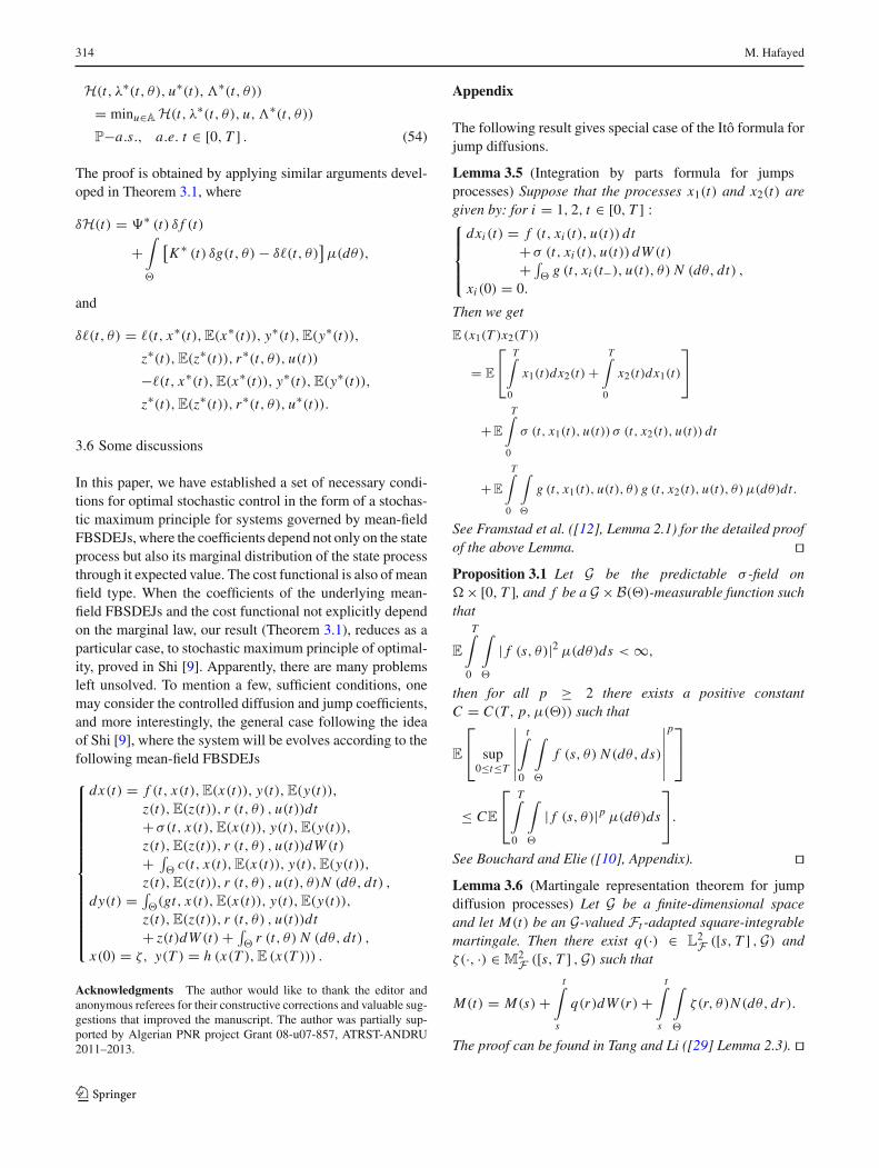
The following result gives special case of the Itô formula forjump diffusions.

Lemma 3.5 (Integration by parts formula for jumpsprocesses) Suppose that the processes x1(t) and x2(t) aregiven by: for i = 1, 2, t ∈ [0, T ] :⎧

⎪

⎪

⎨

⎪

⎪

⎩

dxi (t) = f (t, xi (t), u(t)) dt+ σ (t, xi (t), u(t)) dW (t)+ ∫

�g (t, xi (t−), u(t), θ) N (dθ, dt) ,

xi (0) = 0.

Then we get

E (x1(T )x2(T ))

= E

⎡

⎣

T∫

0

x1(t)dx2(t)+T∫

0

x2(t)dx1(t)

⎤

⎦

+ E

T∫

0

σ (t, x1(t), u(t)) σ (t, x2(t), u(t)) dt

+ E

T∫

0

∫

�

g (t, x1(t), u(t), θ) g (t, x2(t), u(t), θ) μ(dθ)dt.

See Framstad et al. ([12], Lemma 2.1) for the detailed proofof the above Lemma. ��Proposition 3.1 Let G be the predictable σ -field on�× [0, T ], and f be a G × B(�)-measurable function suchthat

E

T∫

0

∫

�

| f (s, θ)|2 μ(dθ)ds < ∞,

then for all p ≥ 2 there exists a positive constantC = C(T, p, μ(�)) such that

E

⎡

⎣ sup0≤t≤T

∣

∣

∣

∣

∣

∣

t∫

0

∫

�

f (s, θ) N (dθ, ds)

∣

∣

∣

∣

∣

∣

p⎤

⎦

≤ CE

⎡

⎣

T∫

0

∫

�

| f (s, θ)|p μ(dθ)ds

⎤

⎦.

See Bouchard and Elie ([10], Appendix). ��Lemma 3.6 (Martingale representation theorem for jumpdiffusion processes) Let G be a finite-dimensional spaceand let M(t) be an G-valued Ft -adapted square-integrablemartingale. Then there exist q(·) ∈ L

2F ([s, T ] ,G) and

ζ(·, ·) ∈ M2F ([s, T ] ,G) such that

M(t) = M(s)+t∫

s

q(r)dW (r)+t∫

s

∫

�

ζ(r, θ)N (dθ, dr).

The proof can be found in Tang and Li ([29] Lemma 2.3). ��

123

A mean-field necessary conditions for optimal stochastic control of FBSDEJs 315

References

1. Shi J, Wu Z (2006) The maximum principle for fully coupledforward–backward stochastic control system. Acta Autom Sin32(2):161–169

2. Shi J, Wu Z (2010) Maximum principle for partially-observed opti-mal control of fully-coupled forward–backward stochastic systems.J Optim Theory Appl 145(3):543–578

3. Xu W (1995) Stochastic maximum principle for optimal controlproblem of forward and backward. J Aust Math Soc Ser B 37:172–185

4. Peng S, Wu Z (1999) Fully coupled forward backward stochasticdifferential equations and application to optimal control. SIAM JControl Optim 37(3):825–843

5. Yong J (2010) Optimality variational principle for controlledforward–backward stochastic differential equations with mixedintial-terminal conditions. SIAM J Control Optim 48(6):4119–4156

6. Ma J, Yong J (1999) Forward–backward stochastic differentialequations and their applications. Lecture notes in mathematics, vol1702. Springer, Berlin

7. Shi J, Wu Z (2010) Maximum principle for forward–backwardstochastic control system with random jumps and application tofinance. J Syst Sci Complex 23:219–231

8. Shi J, Wu Z (2007) Maximum principle for fully coupled Forward-backward stochastic control system with random jumps. In: Pro-ceedings of the 26th Chinese Control Conference, Zhangjiajie,Hunan, China, pp 375–380

9. Shi J (2012) Necessary conditions for optimal control of forward–backward stochastic systems with random jumps. J Stoch Anal258674:50. doi:10.1155/2012/258674

10. Bouchard B, Elie R (2008) Discrete time approximation ofdecoupled forward–backward SDE with jumps. Stoch Proc Appl118(1):53–75

11. Cadenillas A (2002) A stochastic maximum principle for systemwith jumps, with applications to finance. Syst Control Lett 47:433–444

12. Framstad NC, Øksendal B, Sulem A (2004) Sufficient stochasticmaximum principle for the optimal control of jump diffusions andapplications to finance. J Optim Theory Appl 121:77–98

13. Hafayed M, Veverka P, Abbas S (2012) On maximum principleof near-optimality for diffusions with jumps, with application toconsumption-investment problem. Differ Equ Dyn Syst 20(2):111–125

14. Øksendal B, Sulem A (2007) Applied stochastic control of jumpdiffusions, 2nd edn. Springer, Berlin

15. Kac M (1956) Foundations of kinetic theory. In: Proceedings of 3rdBerkeley Symposium on mathematical statistics and probability,vol 3, pp 171–197

16. McKean HP (1966) A class of Markov processes associated withnonlinear parabolic equations. Proc Natl Acad Sci USA 56:1907–1911

17. Shi J (2012) Sufficient conditions of optimality for mean-field sto-chastic control problems. 12th International Conference on con-trol, automation, robotics & vision, (ICARCV 2012), Guangzhou,China, 5–7 Dec 2012

18. Ahmed NU (2007) Nonlinear diffusion governed by McKean-Vlasov equation on Hilbert space and optimal control. SIAM JControl Optim 46:356–378

19. Buckdahn R, Li J, Peng S (2009) Mean-field backward stochas-tic differential equations and related partial differential equations.Stoch Process Appl 119:3133–3154

20. Buckdahn R, Djehiche B, Li J (2011) A general stochastic max-imum principle for SDEs of mean-field type. Appl Math Optim64:197–216

21. Kotelenez PM, Kurtz TG (2010) Macroscopic limit for stochas-tic partial differential equations of McKean-Vlasov type. ProbabTheory Relat Fields 146:189–222

22. Hafayed M, Abbas S (2013) A general maximum principle forstochastic differential equations of mean-field type with jumpprocesses. Technical report

23. Lasry JM, Lions PL (2007) Mean field games. Japan J Math 2:229–260

24. Andersson D, Djehiche B (2011) A maximum principle for SDEsof mean-field type. Appl Math Optim 63:341–356

25. Li J (2012) Stochastic maximum principle in the mean-field con-trols. Automatica 48:366–373

26. Meyer-Brandis T, Øksendal B, Zhou XY (2012) A mean-field sto-chastic maximum principle via Malliavin calculus. Stochastics.84(5–6):643–666

27. Yong J (2011) A linear-quadratic optimal control problem formean-field stochastic differential equations. Technical report

28. Carmona R, Dularue F (2012) Mean-field forward–backward sto-chastic differential equations, Technical report

29. Tang SL, Li XJ (1994) Necessary conditions for optimal controlof stochastic systems with random jumps. SIAM J Control Optim32:1447–1475

123