A Maximum Lifetime Algorithm for Data Gathering Without

Appl. Math. Inf. Sci.7, No. 5, 1705-1719 (2013) 1705

Applied Mathematics & Information SciencesAn International Journal

http://dx.doi.org/10.12785/amis/070508

A Maximum Lifetime Algorithm for Data GatheringWithout Aggregation in Wireless Sensor Networks

Junbin Liang1,2,∗ and Taoshen Li1

1School of Computer and Electronic Information, Guangxi University,Nanning 530004, China2School of Information Science and Engineering, Central South University, Changsha 410083, China

Received: 14 Dec. 2012, Revised: 21 Apr. 2013, Accepted: 23 Apr. 2013Published online: 1 Sep. 2013

Abstract: Data gathering in wireless sensor network (WSN) has attracted a lot of attention in research. Data gathering can be donewith or without aggregation, depending on the degree of correlation among the source data. In this paper, we study the problem of datagathering without aggregation, aiming to conserving the energy of sensor nodes so as to maximize the network lifetime. We model theproblem as one of finding amin-max-weight spanning tree (MMWST), which is shown to be NP-complete. In MMWST, the maximumweight of the nodes is minimized. The weight of a node in the tree equals the ratio of the number of the node’s descendants to thenode’s energy. We propose aΩ(logn/ log logn)-approximation centralized algorithm MITT to construct MMWST without requiringnode location information. Moreover, in order to enable MITT to be used inlarge-scale networks, a new solution that employs theclustering technique is proposed. To the best of our knowledge, MITT isthe first algorithm that constructs MMWST in wireless sensornetworks. Theoretical analyses and simulation results show that MITT can achieve longer network lifetime than existing data gatheringalgorithms.

Keywords: Maximum lifetime, Data gathering, Wireless sensor networks

1 Introduction

A wireless sensor network (WSN) is composed of alarge number of low-cost and low-energy (sensor) nodesthat communicate with each other through multi-hopwireless links [1]. A basic operation in WSN is datagathering, i.e., each node periodically transmits its senseddata to the sink for further processing. Because nodes areoften deployed in remote or inaccessible environments,where replenishing nodes’ batteries is usually impossible,a critical issue in data gathering is to conserve nodes’energies and maximize the network lifetime. The networklifetime is defined as the time until the first node depletesits energy [2].

Data gathering can be categorized by the degree ofcorrelation among the source data [3]. For applications ofstatistical queries in WSN, such as SUM, MAX, MIN,etc., correlation exists among the data sensed by nodes.Therefore, when these data are transmitted, they could beaggregated into one data packet with constant sizeregardless of the number of data sources. This type of

data gathering is called data gathering with aggregation.Data gathering without aggregation refers to the oppositecase, where no data reduction is available and all dataneed to be transmitted to the sink, e.g., collecting videoimages from distant regions of a battlefield. Both types ofdata gatherings have many applications, and attract a lotof research attentions. In this paper, we mainly concernwith data gathering without aggregation. Our goal is tofind an energy-conserving tree at each round of datagathering to maximize the network lifetime.

For data gathering with aggregation, each nodeconsumes energy for receiving data with constant sizefrom all of its children and transmitting the aggregateddata with the same size to its parent. Therefore, theenergy consumption of each node is controlled by thenumber of its children (or its degree in the tree). In orderto maximize the network lifetime, the degrees of all nodesin the tree should be minimized. In [4][5], a(1+ ε)-approximation centralized algorithm is proposedto construct anEnergy-Balanced Minimum Degree DataGathering Tree(EBMDDGT), whereε > 0. In the tree,

∗ Corresponding author e-mail:[email protected]

c© 2013 NSPNatural Sciences Publishing Cor.

http://dx.doi.org/10.12785/amis/070508

1706 J. Liang , T. Li: A Maximum Lifetime Algorithm for Data Gathering...

nodes with higher energy have larger degree, and viceversa. Therefore, the nodes can consume their energyuniformly and maximize the network lifetime. However,if the data cannot be aggregated, a node with smallerdegree in a tree may still need to receive and transmitlarge amounts of data from its descendants. Therefore,EBMDDGT cannot be used in data gathering withoutaggregation to maximize the network lifetime.

For data gathering without aggregation, each nodeconsumes energy for receiving data from all of itsdescendants and transmitting these data together with itsown data to its parent. Therefore, the energy consumptionof each node is controlled by the number of itsdescendants. In order to maximize the network lifetime,the descendant numbers of all nodes in the tree should beminimized. Since a node’s descendant number is oftenmuch larger than its children’s number, the minimizationof all nodes’ descendant numbers is harder than theminimization of all nodes’ degrees.

In traditional network design fields, a shortest pathtree (SPT) can be used to minimize the total energyconsumption of data transmission in the network. This isbecause each node in the SPT can transmit its data to thesink with the minimum number of hops. However, SPTcannot achieve the maximum network lifetime because itdoes not consider how to conserve the energy of anyindividual node, e.g., a node in a shortest path has toalways receive and transmit large amounts of data fromother nodes even if its energy is low.

In this paper, we model the maximum networklifetime problem as one of finding aMin-Max-WeightSpanning Tree (MMWST), which is shown to beNP-complete. In MMWST, the maximum weight of thenodes is smaller than other maximum weights of thenodes in other trees for the network. The weight of a nodeis defined as the ratio of the number of the node’sdescendants to the node’s energy. To the best of ourknowledge, this paper is the first one that researches howto maximize the network lifetime by finding MMWST.

A Ω(logn/ log logn)-approximation centralizedalgorithm MITT (MaxImum lifetime Tree constructionfor data gaThering without aggregation) is proposed forfinding MMWST. MITT starts from an initial tree, whichis constructed by performing a breadth first traversal onthe network. The initial tree is a SPT, which can minimizethe total energy consumption of data transmission in thenetwork but may not be able to maximize the networklifetime. Then, MITT iteratively transfers descendants ofthe nodes with the maximum weight (which are calledbottleneck nodes) to other nodes with smaller weights todecrease the maximum weight. MITT terminates whenthe weights of all bottleneck nodes cannot be decreasedfurther. Compared with existing data gatheringalgorithms, MITT can achieve longer network lifetime.

Moreover, MITT needs the information of nodes’energies and the network topology, which is hard to beacquired in large-scale networks. By employing theclustering technique, a solution for extending MITT to

large-scale networks is proposed. The network is assumedto compose of two kinds of nodes : the regular (sensor)nodes and the cluster-heads. The network is divided intoseveral clusters by the cluster-heads. All cluster-headsform a hierarchical structure rooted at the sink. In eachcluster, MITT is performed by the cluster-head andconstructs a min-max-weight spanning tree for the cluster.Each node in the cluster transmits its data to itscluster-head by the tree, and the cluster-head isresponsible for transmitting these data to the sink. By thisway, MITT can be implemented in a large-scale networkeasily. Since the cost of cluster-heads is much higher thanthe regular nodes, the upper bound of the number ofcluster-heads that should be used to achieve the maximumnetwork lifetime is analyzed.

The remainder of this paper is organized as follows.Section II reviews related work on data gathering. SectionIII describes the system model and formulates theproblem. Section IV describes our algorithm. Simulationresults are presented in section V, and Section VIconcludes this work.

2 Related work

Recently, the problem of efficient data gathering inWSN has been investigated extensively. Existingprotocols can be classified into three categories :cluster-based protocols, chain-based protocols andtree-based protocols. For continuous monitoringapplications with a periodic traffic pattern, tree-basedtopology is often adopted because of its simplicity [6].Therefore, the tree-based protocols are our main concern.

(1) In cluster-based protocols (e.g., LEACH [7],HEED [8], EECJ [9], MCMC [10], CDE [11], CDC [12],and LCTSR [13], etc.), a subset of nodes in the networkare selected as cluster heads by probability, and othernodes join the closest cluster head from them to form aVoronoi-based topology. Cluster-based protocols are easyto be implemented and managed, but they have somedisadvantages such as asymmetry distribution of thecluster heads, heavy load on the cluster heads, etc. Inaddition, the sizes of the clusters are hard to be controlled.

(2) In chain-based protocols (e.g., PEGASIS [14],DRAEM [15], CHIRON [16], EECC [17], andCREEC [18], etc.), all nodes in the network are organizedas a chain. One of these nodes is selected as a head tocommunicate with the sink directly, and other nodestransmit their data to the head through the chain.Chain-based protocols enable each node to communicatewith its closest neighbor. However, the long chain causesa large delay in data gathering and the head has thehighest burden of relaying data.

(3) In tree-based protocols, all nodes in the networkare organized as a tree. Each node in the tree receives datafrom all of its children. Then, it transmits its own data andthe received data to its parent. According to the way ofconstructing a tree, the tree-based protocols for data


Appl. Math. Inf. Sci.7, No. 5, 1705-1719 (2013) /www.naturalspublishing.com/Journals.asp 1707

gathering without aggregation can be classified into threecategories : linear programming based protocols, growthbased protocols and improvement based protocols.

In linear programming based protocols, the problemof finding a maximum lifetime data gathering tree ismodeled as a maximum flow problem [19] with energyconstraints at the nodes. Then, the problem is solved byan integer program with linear constraints. Thoughfinding a feasible solution to the integer program is stillNP-complete, it can obtain an approximation result forthe problem by relaxing some integrality conditions.MLDR [20] and RSM-MLDA [21] are typical linearprogramming based protocols. However, they assume thatthe locations of the nodes and the sink are known, whichare hard to be acquired because the nodes and the sink areseldom equipped with expensive GPS devices. Moreover,they assume that each node has the ability to transmit itspacket to any other node in the network or directly to thesink, which is unrealistic in a large-scale network.In [22][23][24], the maximum lifetime problem insensor-target surveillance networks is researched. Theproblem is to schedule the sensors to watch the targetsand forward the sensed data to the sink, such that thelifetime of the surveillance network is maximized. Theyfirstly compute the maximum lifetime of the surveillancesystem and a workload matrix by using the linearprogramming technique. Then, they decompose theworkload matrix into a sequence of schedule matrices thatcan achieve the maximum lifetime. Finally, they constructthe sensor surveillance trees based on the above obtainedschedule matrices, which specify the active sensors andthe routes to pass sensed data to the sink.

For growth based protocols, their basic ideas aresimilar to the Prim’s algorithm forminimum spanningtree (MST). Each edge in the network is assigned aweight. The data gathering tree is initialized bycontaining only the sink node. Then, the tree is grown byadding selected edges one by one until it spans all nodes.The selected edge is from a node in the tree to anothernode not in the tree. The key difference in these protocolsis how to define each edge’s weight and how to add aproper edge to the tree at each time. In PEDAP [25], theweight of each edge is defined as the transmission costbetween the edge’s two end nodes. At each time, PEDAPadds an edge with the minimum weight to the tree.However, PEDAP does not consider nodes’ energies andcannot achieve energy-awareness. PEDAP-PA [25]improves PEDAP by considering each node’s energyduring the tree construction. The weight of each edge isdefined as the ratio of the transmission cost between thetwo end nodes to the residual energy of the sending node.PEDAP-PA achieves an approximation ratio ofΩ(logn),where n is the number of nodes in the network.MLDGA [ 26] and MNL [27] improve PEDAP-PA bydesigning different edge weights. In MLDGA, the weightof each edge is defined as the ratio of the minimumlifetime of the edge’s two end nodes to the transmissioncost between the two nodes. At each time, an edge with

the maximum weight is added to the tree. In MNL, anedge is added to the tree if it can maximize the minimumresidual energy of the nodes of the new tree. MLDGA andMNL also achieve the approximation ratio ofΩ(logn).

Improvement based protocols start with an initialfeasible solution, and then make improvements by addingand deleting edges as long as improvements are possible.To the best of our knowledge, LOCAL-OPT [28] is theonly one improvement based protocol that constructs atree for data gathering without aggregation. It starts froman arbitrary treeT0 with lifetime L0. Then, it tries tochange each node’s parent in the tree to one of the node’sneighbors in the network to find a new treeT1, which haslifetime L1 > L0. If T1 is found, another new treeT2 thathas lifetimeL2 > L1 is found by the same way. The aboveprocess of finding new trees is executed iteratively, until atreeTi with lifetime Li is found and there is no a treeTjwith lifetime L j > Li can be found. LOCAL-OPTachieves an approximation ratio ofΩ(logn/ log logn),which is the current best result for tree construction indata gathering without aggregation. However,LOCAL-OPT does not consider the situation thatTj canbe found by changing parents of multiple nodes inTi atthe same time. Moreover, in above optimization processof changing each node’s parent to one of the node’sneighbors to find a new tree, LOCAL-OPT does not usethe nodes that are not the changed node’s neighbors toenlarge the algorithm’s optimization range.

In this paper, a new improvement based protocolMITT that can achieve better performance of finding amaximum lifetime data gathering tree than LOCAL-OPTis proposed. The system model and problem statementthat MITT considers are described as follows.

3 System model and problem statement

3.1 Network model

Assume thatv1,v2, . . . ,vn are sensor nodes (or nodes)in a WSN andv0 is the sink. All nodes are randomlydeployed over anM × M field. The network forms aconnective undirected graphG(V,E), whereV is the setof the nodes and the sink, andE is the set of edges.|E| = m is the number of edges. There is an edge(vi ,v j)in E if the nodesvi and v j are within each other’scommunication range. Each node has different initialenergy. The network has following characteristics :

(1) The network is static, i.e., all nodes and the sink arestationary after deployment.

(2) The sink has infinite power supply and powerfulcomputation ability.

(3) All nodes have the same transmission range.Each node mainly consumes energy in

communication, and the amount of energy required totransmit, receive one bit of data isEtx, Erx respectively.The energy consumed by nodes in computing and sensing


www.naturalspublishing.com/Journals.asp


is negligible [10]. At each round, each node generateslbits data.

3.2 Definitions

Before diving into the problem of finding a maximumlifetime tree for data gathering without aggregation, somefundamental definitions and notations are given, whichwill be used throughout this paper .

De f inition1 : A round is defined as the process ofgathering all the data from nodes to the sink, regardless ofhow much time it takes [25].

De f inition2 : For each nodevi that has S(T,vi)descendants in a treeT, the size of data that it receives ateach round isS(T,vi)l and the size of data that it needs totransmit is(S(T,vi)+1)l .

De f inition3 : At each round, the amount of energyC(T,vi) that each nodevi consumes in a treeT is :

C(T,vi) = S(T,vi)lErx +(S(T,vi)+1)lEtx

= S(T,vi)l(Erx +Etx)+ lEtx(1)

De f inition4 : The lifetime of a nodevi in a treeT isdefined as the number of rounds that the node can receivedata from all of its descendants and transmit these datatogether with its own data to its parent :

Lnode(T,vi) = ⌊E(vi)

S(T,vi)l(Erx +Etx)+ lEtx⌋ (2)

De f inition5 : The lifetime of a treeT is defined as thenumber of rounds that the tree can sustain until the firstnode in the tree depletes its energy :

Ltree(T) = mini=1,...,n

Lnode(T,vi) (3)

De f inition6 : The network lifetime is defined as thenumber of rounds that the network can perform datagathering until the first node in the network depletes itsenergy.

In fact, an alternative definition of the networklifetime that can be used is the number of rounds that thenetwork can perform data gathering until a certainpercentage of nodes in the network deplete their energies.That is because the nodes are often deployed in a networkdensely, the quality of the network is not affected until asignificant amount of nodes die. In [30], it is shown thatthis definition is actually quite similar in nature toDefinition 6. Therefore, Definition 6 is used in this paperfor simplicity.

De f inition7 : Let TS(G) = T1, . . . ,Tz be the set ofspanning trees in the network andw(Ti) be the weight of atreeTi in TS(G), wherew(Ti) equals the maximum weightof the nodes in the treeTi , i.e., w(Ti)= max

i=1,...,zj=1,...,n

w(Ti ,v j). A

spanning treeTi is called amin-max-weight spanning treeif its weight is the minimum among all trees inTS(G), i.e.,w(Ti)= min

T∈TS(G)w(T).

3.3 Problem statement

(a) The problem of finding a min-max-weight spanningtree (PMMWST)

In tree-based protocols, a tree can be used for a periodof time or be reconstructed at each round, depending onspecific applications. If a tree is used until the first nodedepletes its energy, the network lifetime is equal to thelifetime of the tree. If a tree is reconstructed at each roundor after it is used for several rounds, the network lifetimeis decided by the trees that are constructed.

No matter whether the tree is reconstructed or not, itis expected that the tree can effectively conserve nodes’energies at each round so as to maximize the networklifetime. A tree with maximum lifetime can achieve aboveexpectation, so it is our main concern.

For a networkG, there exists multiple possible trees.Our goal is to find a tree with the maximum lifetime :

maxT∈TS(G)

Ltree(T) (4)

According to Definitions 4 and 5, Formula (4) can bedefined as :

maxT∈TS(G)

mini=1,...,n

⌊E(vi)

S(T,vi)l(Erx +Etx)+ lEtx⌋ (5)

In Formula (5), sinceErx andEtx are constant,S(T,vi)is the main optimization objective. Being extracted theconstantErx and Etx from the denominator, the problemfor solving Formula (5) is transformed to a new problem :

maxT∈TS(G)

mini=1,...,n

E(vi)

S(T,vi)+c(6)

wherec = Etx/(Erx +Etx). In Formula (6), the goal is tomaximize the minimum ofE(vi)/(S(T,vi)+c), wherei =1, . . . ,n. In order to achieve this goal, a node with largerenergy (largerE(vi)) should take more responsibilities byserving more descendants (largerS(T,vi)) in a tree, andvice versa.

In Formula (6), the variable S(T,vi) is in thedenominator, which is not convenient to be analyzed.Hence, the problem for solving Formula (6) istransformed to another problem by changingE(vi)/(S(T,vi)+c) to (S(T,vi)+c)/E(vi) as follows :

minT∈TS(G)

maxi=1,...,n

S(T,vi)+cE(vi)

(7)

Each node vi in T is given a weightw(T,vi)=(S(T,vi) + c)/E(vi), then Formula (7) istransformed into :

minT∈TS(G)

maxi=1,...,n

w(T,vi) (8)



v1 v2 v3 vn-2

S1 S2 Sk-1

vn-1 vn

Sk

u1 u2

root

FIGURE 1 Reduction from SET-COVER to our problem

Note that Formula (8) has the same goal with theinitial problem of solving Formula (4). From Formula (8),the initial problem of finding a maximum lifetime tree istransformed to the problem of finding a min-max-weightspanning tree, i.e., PMMWST. Next, we will establish thehardness of PMMWST.

(b) Hardness of PMMWST

The decision version of PMMWST is : Given anetwork G(V,E) and node energies, does there exist aspanning tree in which the maximum weight of the nodesis w?

Theorem 1 : The decision version of PMMWST isNP-complete.

Proo f : The proof employs the minimum set coverproblem [29] (SET-COVER for short), which is known tobe NP-complete. PMMWST’s decision version is shownto be NP-complete as follows.

PMMWST’s decision version is clearly in NP. Givena tree and node energies, it is easy to verify whether themaximum weight in the tree reachesw. In order to provethat PMMWST’s decision version is NP-Complete, areduction from SET-COVER to it is shown.

Given an element setS = v1,v2, . . . ,vn and acollection of subsetsC = S1,S2, . . . ,Sk of S, thedecision version of SET-COVER is to determine whetherthere is a selection ofK subsets fromC such that theunion of K subsets cover all then elements, where1 ≤ K ≤ k. Given an instance of SET-COVER, aninstance of the network can be constructed in polynomialtime as follows.

The nodes in the network are arranged in four rows, asshown in Figure 1. The first row just has a root node (thesink), which has unlimited energy supply. The second rowconsists of two nodes :u1 with energy(n+K)+c andu2with energy(k−K)+c. The two nodes are used to decidewhich subsets will be in the set cover and which will not.

Both of the two nodes are connected to the root node.There arek nodes corresponding toS1,S2, . . . ,Sk in thethird row, and each node corresponding toSj has2(|Sj |+c) units of energy, where 1≤ j ≤ k and|Sj | is thesize ofSj . Thek nodes are connected to bothu1 andu2. Inthe fourth row,n nodes with energy 2c are correspondingto then elements ofS. For each node corresponding to theelement vi , there is an edge from it to the nodecorresponding toSj if vi is in Sj , where 1≤ i ≤ n.

In Figure 1, each node corresponding tovi or each nodecorresponding toSj has a weight at most 1/2. The nodesthat can achieve larger weights in the instance are nodesu1andu2. Now, it can be claimed that there exists a spanningtree in which the maximum weight of the nodes is 1 if andonly if a set cover of sizeK exists.

Suppose that there exists a set cover of sizeK. Thenthe tree can be constructed as follows. The data from theK third row nodes and then fourth row nodes can be routedthroughu1 to the root. The data from rest of thek−K thirdrow nodes can be routed throughu2. Only by this way, bothu1’s andu2’s weights achieve 1, i.e., the maximum weightof the nodes in the tree is 1.

Conversely, if there is a spanning tree in which themaximum weight of the nodes is 1, then it is easy toconstruct a set cover for the SET-COVER instance. Thatis the union of the subsets corresponding to theK thirdrow nodes, which contains all the elements inS.

Since PMMWST is hard, an approximate solutionneeds to be found. In this paper, an approximationalgorithm MITT is proposed to solve PMMWST. Detailsof the algorithm are shown as follows.

4 MITT algorithm

4.1 Algorithm description

Firstly, an initial treeT is constructed in the networkGas follows :

(1) Initially, there is only one nodev0 in the treeT, andit is in level 1 ofT.

(2) All neighbors ofv0 are added toT as its children,and these nodes are in level 2 ofT.

(3) The nodes in levelh of T are sorted in descendingorder according to their energies, whereh≥ 2. Accordingto the order, each node in levelh picks all of its neighborsthat are not in the tree as its children in turn. When allneighbors of the nodes in levelh are added into the treeT,the levelh+1 of the tree is formed.

Step (3) is executed iteratively and terminates when allnodes in the network are added to the tree. When step (3)terminates,T is got. Based on the initial tree, amin-max-weight spanning treeis constructed as follows.

Given an arbitrary variableϕ >0, all nodes inT areclassified into three disjoint subsetsV1,V2 andV3 :

(1) V1 = vi |w(T)−ϕ < w(T,vi) ≤ w(T),vi ∈ V. V1contains the nodes whose weights are equal to or close to




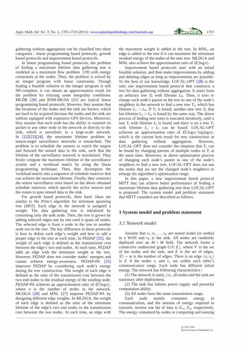
Function Capacity(T,x)1. if (x is the sink)x.capacity=n ;

// n is the number of nodes in sensor network2. else casex∈V1 x.capacity=-1 ;3. case x ∈ V2 x.capacity = min0,x.parent.capacity ;

4. casex ∈ V3 x.capacity= min⌊(w(T) − ϕ −w(T,x)) E(x)−c⌋,x.parent.capacity ;

5. 6. For each childy of x in treeT7. Capacity(T, y) ;8.

FIGURE 2 Function Capacity(T, x)

the weightw(T) of the treeT (or the maximum weight ofthe nodes in the tree). These nodes are called “bottlenecknodes”.

(2) V2 = vi |w(T)−ϕ −1/E(vi)< w(T,vi)≤ w(T)−ϕ,vi ∈V. Each node inV2 will become abottleneck nodeif the number of its descendants is increased by one. Thenodes inV2 are called “sub-bottleneck nodes”.

(3) V3 =V −V1−V2. V3 contains all remaining nodes,and these nodes are called “rich nodes”. Each node inV3will not become abottleneck nodeeven if the number ofits descendants is increased by one.

However, a node inV3 does not mean that it can beadded more descendants. That is because some of thenode’s ancestors may be inV1 or V2, and they wouldbecome new bottleneck nodes if the number of the node’sdescendants is increased. To represent this property, anattributecapacity is used to denote a node’s ability forserving more descendants according to its weight and itsancestors’ weights.

For abottleneck node, it has larger weight than othernodes. Therefore, it and its descendants should not beadded more descendants. As a result, if a node is abottleneck nodeor a bottleneck node’s descendant, itscapacityis set to -1.

For a sub-bottleneck node, its descendant numbershould not be increased too. Therefore, if a node is asub-bottleneck node, itscapacity is set to the minimumbetween 0 and its ancestors’capacities.

If a nodevi is a rich node, its capacityis equal to theminimum between⌊(w(T)−ϕ −w(T,vi))E(vi)− c⌋ andits ancestors’ capacities. Note that⌊(w(T) − ϕ − w(T,vi))E(vi) − c⌋ is the number ofdescendants thatvi can further afford.

MITT can compute all nodes’capacitiesby traversingthe tree in depth first order once. A Function Capacity(T,x)is defined to compute thecapacitiesof nodes in a treeTrooted at a nodex, which is shown in Figure 2.

After all nodes’ capacities are got, a transferringoperation is performed on eachbottleneck node vi to tryto transfer some ofvi ’s descendants (the number of these

descendants iss) to another nodev j that is not vi ’sdescendant to decreasevi ’s weight. In the transferringoperation, there are 3 cases that may happen as follows :

(1)if v j ’s capacityis larger thans, vi can transfer itssdescendants tov j directly, i.e., v j becomes thesdescendants’ new ancestor.

(2)If v j ’s capacityequals 0, it means thatv j is in asub-tree rooted at asub-bottleneck node vk, wherevk andvi may be the same node andvk has the characteristicsthat vk.capacity==vi .capacity andvk.parent.capacity> vi .capacity. Since vk’s capacitydecidesv j ’s capacity, vk’s capacity is increased firstly.By performing the transferring operation onvkrecursively,vk’s capacitycan be increased. Therefore, ifv j ’s capacitybecomes larger thans after vk’s capacityisincreased,vi can transfer itssdescendants tov j .

(3)If v j ’s capacity is not larger thans, vi does nottransfer itssdescendants tov j .

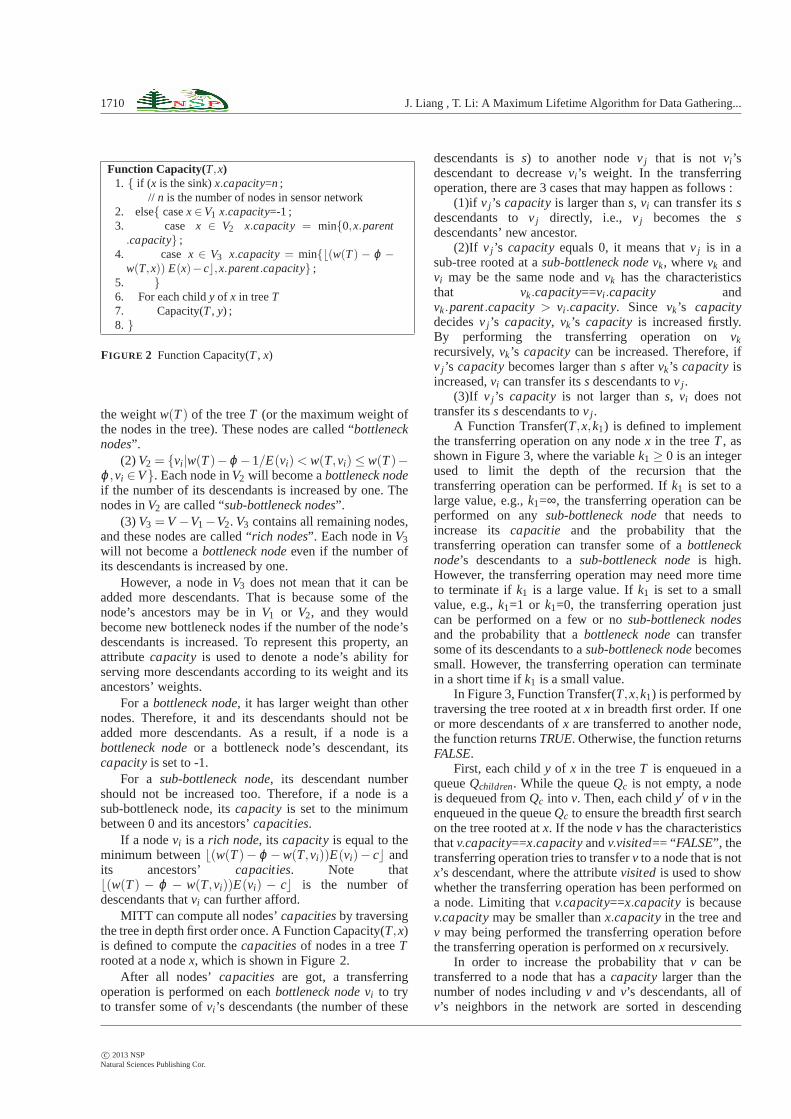
A Function Transfer(T,x,k1) is defined to implementthe transferring operation on any nodex in the treeT, asshown in Figure 3, where the variablek1 ≥ 0 is an integerused to limit the depth of the recursion that thetransferring operation can be performed. Ifk1 is set to alarge value, e.g.,k1=∞, the transferring operation can beperformed on anysub-bottleneck nodethat needs toincrease its capacitie and the probability that thetransferring operation can transfer some of abottlenecknode’s descendants to asub-bottleneck nodeis high.However, the transferring operation may need more timeto terminate ifk1 is a large value. Ifk1 is set to a smallvalue, e.g.,k1=1 or k1=0, the transferring operation justcan be performed on a few or nosub-bottleneck nodesand the probability that abottleneck nodecan transfersome of its descendants to asub-bottleneck nodebecomessmall. However, the transferring operation can terminatein a short time ifk1 is a small value.

In Figure 3, Function Transfer(T,x,k1) is performed bytraversing the tree rooted atx in breadth first order. If oneor more descendants ofx are transferred to another node,the function returnsTRUE. Otherwise, the function returnsFALSE.

First, each childy of x in the treeT is enqueued in aqueueQchildren. While the queueQc is not empty, a nodeis dequeued fromQc into v. Then, each childy′ of v in theenqueued in the queueQc to ensure the breadth first searchon the tree rooted atx. If the nodev has the characteristicsthatv.capacity==x.capacityandv.visited== “FALSE”, thetransferring operation tries to transferv to a node that is notx’s descendant, where the attributevisited is used to showwhether the transferring operation has been performed ona node. Limiting thatv.capacity==x.capacity is becausev.capacitymay be smaller thanx.capacityin the tree andv may being performed the transferring operation beforethe transferring operation is performed onx recursively.

In order to increase the probability thatv can betransferred to a node that has acapacity larger than thenumber of nodes includingv and v’s descendants, all ofv’s neighbors in the network are sorted in descending



Function Transfer(T,x,k1)1. for(each childy of nodex in the treeT)2. enqueue(Qc, y) ; //enqueue the nodey in a queueQc3. while (Length(Qc)> 0)4. dequeue(Qc, v) ; //dequeue a node fromQc into v5. for(each childy′ of nodev in the treeT)6. enqueue(Qc, y′) ;7. if (v.capacity==x.capacityandv.visited==“FALSE”)8. all neighbors ofv in the network are first sorted in

descending order according to theircapacities, and thenthey are enqueued in a queueQn ;

9. while (Length(Qn)> 0)10. dequeue(Qn, z) ;11. if(nodez is not a descendant of nodex in T)12. casez.capacity> S(T,v)13. ChangeParent(v, z) ;14. returnTRUE;15. case (z.capacity==0)&& (k1 >0)16. find the ancestorvk of z that has

the characteristics vk.capacity==z.capacity andvk.parent.capacity> z.capacity;

17. if(vk.visited==“FALSE”)18. vk.visited=“TRUE” ;19. if ( Transfer(T,vk,k1-1) && z.capacity>

S(T,v))20. ChangeParent(v,z) ;21. returnTRUE;22. 23. 24. case (z.capacity≤ S(T,v)) break ;25. //endif26. //endwhile27. //endif28. //endwhile29. returnFALSE;

Function ChangeParent(v,z)1. w= v.parent;2. v.parent= z;3. updateS(T,vi) for each nodevi that isv’s old ancestor

or v’s new ancestor, and letvi .visited=“FALSE” ;4. Capacity (T,v0) ;

FIGURE 3 Function Transfer(T,x,k1)

order according to theircapacities and then they areenqueued in a queueQn. While the queueQn is notempty, a node is dequeued fromQn into z. If z is not adescendant of nodex in the treeT, there are three casesthat may happen as follows :

(1) If z.capacity> S(T,v), v can be transferred tozdirectly, i.e.,v takesz as its new parent. Since the tree ischanged, each node that isv’s old ancestor orv’s newancestor sets itsvisited attribute to “FALSE”. Then, thecapacities of all nodes in the tree are re-computed.Finally, the function returnsTRUE.

(2) If z.capacity==0, v cannot be transferred tozdirectly. Therefore, the root nodevk of the sub-treecontaining z should be found, which has thecharacteristics that vk.capacity==z.capacity andvk.parent.capacity > z.capacity. Ifvk.visited==“FALSE”, the transferring operation isperformed on vk recursively, i.e., FunctionTransfer(T,vk,k1) is executed. If some ofvk’s descendantsare transferred andz’s capacity is larger thanS(T,v), vcan be transferred toz. Otherwise,v does not transfer toz.If the transferring operation succeeds and the tree ischanged, each node that isv’s old ancestor orv’s newancestor sets itsvisited attribute to “FALSE”. Then, thecapacities of all nodes in the tree are re-computed.Finally, the function returnsTRUE.

(3) If z.capacity≤ S(T,v), v cannot be transferred toany of its neighbors. Therefore, the function stops thecurrent transferring operation onv and continues todequeue another node fromQc into v to re-perform aboveoperations.

If z is a descendant of nodex in the treeT, v doesnot transferred tozand another node is dequeued fromQninto z. Then,v tries to be transferred to the newz. If thequeueQn is empty andv cannot be transferred to any oneof its neighbors, another node is dequeued fromQc into vto re-perform above above operations. If the queueQc isempty and there is no a node in the tree rooted atx can betransferred, the function returnFALSE.

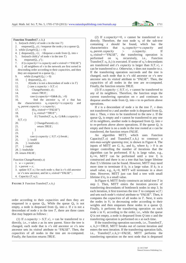
An algorithm MITT, which uses FunctionCapacity(T,x) and Transfer(T,x,k1) to construct amin-max-weight spanning tree, is shown in Figure 4. Theinputs of MITT areG, k1, and k2, wherek2 > 0 is aninteger controlling the number of iterations that thealgorithm can be performed. Ifk2 is large value, e.g.,k2=∞, MITT can be performed until a treeTi isconstructed and there is no a tree that has larger lifetimethanTi ’s lifetime can be found. However, MITT may needmore time to terminate ifk2 is a large value. Ifk2 is asmall value, e.g.,k2=0, MITT will terminate in a shorttime. However, MITT just can find a tree with smalllifetime if k2 is a small value.

In Figure 4, MITT firstly constructs an initial treeT instep 1. Then, MITT enters the iteration process oftransferring descendants of bottleneck nodes in step 3. Ineach iteration, it first traverses the treeT to computew(T)and sets each node’svisitedattribute to “FALSE”. Then, itcomputes thecapacitiesof all nodes inT. Next, it sortsthe nodes inV1 in decreasing order according to theirweights and then enqueues these nodes in a queueQ.Finally, it performs the transferring operation on eachnodex in V1 according to the order, i.e., while the queueQ is not empty, a node is dequeued fromQ into x and thetransferring operation is performed onx at each time.

If the transferring operation succeeds, i.e., Transfer(T,x, k1)==TRUE, MITT breaks out of current iteration andenters the next iteration. If the transferring operation fails,i.e., Transfer(T,x,k1)==FALSE, MITT performs thetransferring operation on the next node that is dequeued




Algorithm MITTInput : NetworkG(V,E), the parametersk1 andk2Out put : a min-max-weigh spanning treefor datagathering without aggregation

1. construct an initial treeT ;2. Ischanged=“TRUE” ;3. while((Ischanged==“TRUE” ) && ( k2 >= 1) )4. Ischanged=“FALSE” ; k2 = k2−1 ;5. traverse the treeT to computew(T), and let each

nodev.visited=“FALSE” ;6. Capacity (T,v0) ;7. all the nodes inV1 are first sorted in descending order

according to their weights, and then they are enqueuedin a queueQ ;

8. while (Length(Q)> 0)9. dequeue(Q, x) ;10. if(Transfer(T,x,k1))11. Ischanged=“TRUE” ;12. break ;13. //endif14. //endwhile15. //endwhile

FIGURE 4 MITT Algorithm

from Q, and so on. If the queueQ is empty, it means thatthe weights of all bottleneck nodes inV1 cannot bedecreased and the algorithm MITT terminates.

In MITT, each node’svisited attribute is firstly set to“FALSE” when the algorithm is executed. If a nodevi isperformed the transferring operation, i.e., FunctionTransfer(T,vi ,k1) is executed, itsvisitedattribute is set to“TRUE”. When the number of the node’s descendants ischanged, i.e., the transferring operation succeeds, thenode’svisitedattribute becomes “FALSE” again. For eachnode, it would not be performed the transferring operationagain if its visited attribute equals “TRUE”. Therefore,the visited attribute prevents each node from beingperformed the transferring operation repeatedly, whichcan eliminate the appearance of dead lock.

Proposition 1 : For MITT, each iteration will befinished in polynomial time. When MITT terminates, it isperformed at mostO(n2(1+1/(ϕEmin))) iterations.

Proo f : As shown in Figure 4, step 1 is to constructan initial treeT. It starts with a tree that contains only thesink node, and then selects a node that is not in the tree tojoin the tree at each time iteratively. Hence, aftern timesof selecting, all nodes are added into the tree.

Steps 3-15 describe the process of transferringdescendants of bottleneck nodes in the treeT byiterations. In each iteration, MITT needs to traverse thesub-trees rooted at thebottleneck nodes(may be includeother sub-trees rooted atsub-bottleneck nodes) and checkneighbors of the nodes in these sub-trees, which costsO(nm) time. Computing thecapacitiesof all nodes in the

treeT costO(n) < O(nm) time. Therefore, each iterationcostsO(nm) time.

On the other hand, the attributecapacityensures thatthe transferring operation just transfers descendants of thenodes with larger weights to the nodes with smallerweights and there is no new bottleneck nodes will begenerated after the transferring. Therefore, the maximumweight of the nodes in the network can only be decreased.When the weights of all bottleneck nodes cannot bedecreased, MITT terminates. The largest number ofiterations that MITT is performed when it terminates isanalyzed as follows.

Let w∗ denote the weight of the optimal tree, whichequals the maximum weight of the nodes in the optimaltree. In MITT, a bottleneck node can be changed to asub-bottleneck node or a rich node, if its weight isdecreased to a value that is smaller thanw(T)−ϕ. Whenthe weights of all bottleneck nodes are smaller thanw(T)−ϕ, w(T) is decreased by at leastϕ. When MITTterminates, it is performed at most⌈(w(T)−w∗)/ϕ⌉Z <⌈((n + c)/Emin − 0)/ϕ⌉Z = ⌈(n + c)/(ϕEmin)⌉Ziterations, whereZ is the number of iterations that MITTneeds to decrease the weights of all bottleneck nodes tovalues that are smaller thanw(T) − ϕ andEmin = min

i=0,...,nE(vi).

For a bottleneck nodevi , its weight will be decreasedby 1/E(vi) if one of its descendants is transferred.Therefore, after at most⌈ϕ/(1/E(vi))⌉ = ⌈ϕE(vi)⌉iterations, its weight will be smaller thanw(T)− ϕ. Inorder to decrease the weights of all bottleneck nodes tovalues that are smaller thanw(T)−ϕ, the largest numberof iterationsZ′ that MITT needs to be performed is :

Z′ = ∑vi∈V1

⌈ϕE(vi)⌉ ≤ ∑vi∈V1

(ϕE(vi)+1)

≤ ϕ ∑vi∈V1

E(vi)+ |V1|(9)

For any bottleneck node vi , there isw(T) − ϕ < w(T,vi) ≤ w(T). Therefore, we havew(T) − ϕ < (S(T,vi) + c)/E(vi) ⇒(w(T)−ϕ)E(vi)< S(T,vi)+c. SinceS(T,vi)< n, for allbottleneck nodes we have :

(w(T)−ϕ) ∑vi∈V1

E(vi)< ∑vi∈V1

(S(T,vi)+c)

< n2+cn

⇒ ∑vi∈V1

E(vi)< (n2+cn)/(w(T)−ϕ)

(10)



Since|V1|< n andc=Etx/(Erx+Etx)< 1, Formula (9)is transformed into a new form as follows by combiningwith Formula (10) :

Z′ ≤ ϕ ∑vi∈V1

E(vi)+ |V1|

< ϕ(n2+cn)/(w(T)−ϕ)+n

< (ϕn2+nw(T))/(w(T)−ϕ)

(11)

Notice thatw(T)≤ ⌈(n+c)/Emin⌉ andZ ≤ Z′, there isZ = O(n(ϕEmin+1)). Therefore, when MITT terminates,it is performed at most⌈(n+ c)/(ϕEmin)⌉Z = O(n2(1+1/(ϕEmin))) iterations.

4.2 Time complexity analysis

Theorem 2 : The time complexity of MITT isO(n3m(1+1/(ϕEmin))).

Proo f : In Figure 4, step 1 costsO(n) time toconstruct the initial tree by traversing the network inbreadth first order. In step 3-15, the algorithm isperformed at mostO(n2(1+ 1/(ϕEmin))) iterations, andeach iteration costsO(nm) time. Therefore, the total timespent in step 3-15 isO(n2(1 + 1/(ϕEmin)))O(nm)=O(n3m(1 + 1/(ϕEmin))).Based upon the above analysis, the time complexity of thewhole algorithm isO(n3m(1+1/(ϕEmin))).

4.3 Approximation ratio

In this subsection, the approximation ratio of MITT isanalyzed by a network instance as follows.

Theorem 3 : The MITT algorithm can achieve anapproximation ratio of at leastΩ(logn/ log logn).

Proo f : Consider a networkG that is shown in Figure5(a). Assume that each node hase units of energy andgenerates one bit of data at each round. Moreover, eachnode will consumea, b units of energy in receiving,sending one bit of data. An optimal tree is shown inFigure 5(b), in which the bottleneck nodes have just onechild. The lifetime of the optimal tree isLopt = e/(a + 2b). Figure 5(c) shows the initial treeconstructed by MITT, in which each bottleneck node has4 children.

For MITT, whenk1=0, the function Transfer(T,x,k1)cannot be performed on anysub-bottleneck node, i.e.,MITT cannot transfer abottleneck node’s descendants toa sub-bottleneck nodeby firstly transferring somedescendants of thesub-bottleneck nodeto a third node toincrease thesub-bottleneck node’s capcity. Therefore, inone of the worst cases, the initial tree is changed to alocally optimal tree, as shown in Figure 5(d), where thelocally optimal tree is a tree that MITT constructs and

(a) Network topology

(b) The optimal tree

(c) The initial tree

(d) A tree constructed by MITT whenk1=0

FIGURE 5 A network topology and some of its trees

MITT cannot find another tree that has larger lifetimethan the tree.

In Figure 5(d), the bottleneck node on the leftmost ofthe middle row hasq=3 children. Therefore, the lifetimeof the locally optimal tree isLMITT=e/(q(a+ b)+ b). Inthis situation, MITT achieves an approximation ratioA=Lopt/LMITT=(q(a+b)+b)/(a+2b).

Clearly, the construction of the locally optimal treecan be extended to arbitraryq. Consider the followingrecurrence. LetN( f ) be the number of nodes that have0 ≤ f ≤ q children. From Figure 5(d), there areN(3)=1,N(2)=2, N(1)=4 and N(0)=4. Therefore, a recurrentinference is formed as follows :N(q)=1, N(q−1)=q−1,N(q−2)=(q−1)N(q−1) andN(q−3)=(q−2)N(q−2).From the above inference, the functional form ofN( f ) isgot :

N( f ) =

( f +1)N( f +1), if 0 ≤ f ≤ q−2,q−1, if f = q−1,1, if f = q.

(12)




For the sinkv0 :1. v0 is assigned a levelLevel0=0 ;2. v0 broadcasts a packetpacket(v0)=(v0,Level0) that

contains its ID and its level to its neighbors ;

For each nodevi :1. if (vi receives a packetpacket(v j )=(v j ,Levelj ) andvi

does not set a node as its parent)2. vi setsv j as its parent ;3. Leveli=Levelj+1 ;4. vi broadcasts a packetpacket(vi)=(vi ,Leveli) to its

neighbors ;5.

FIGURE 6 The scheme of constructing a hierarchical structurewith the sink being the root for all nodes in the network

Since n >q

∑f=1

f N( f )=O(qq), q=Ω(logn/ log logn).

Therefore, the approximation ratio of MITT isA= Ω(logn/ log logn).

Whenk1 > 0, MITT can achieve higher performancethan MITT with k1=0. For example, in Figure 5, thelocally optimal tree can continue to be optimized to a treewith higher lifetime or the optimal tree by MITT ifk1 > 1. Therefore, MITT can achieve an approximationratio of at leastΩ(logn/ log logn).

4.4 Implementation of MITT

Since some nodes may die for depleting their energyor physical damage, and some other nodes may besupplemented to the network at some time, the set of thenodes may be changed at each round. In order to adapt tothe dynamic characteristic of the network, the tree isreconstructed at each round. The implementation ofMITT is similar to LEACH and IAA, where each roundbegins with a set-up phase, and then is followed by asteady-state phase. MITT is performed to compute amin-max-weight spanning treein the set-up phase, anddata gathering based on the tree is carried through in thesteady-state phase.

In the set-up phase, the sink firstly collects theinformation of all nodes’ energies and neighbors. Sinceeach node does not know the path from it to the sink, itcannot transmit its information to the sink. In order tosolve this problem, a scheme is proposed to construct ahierarchical structure with the sink being the root for allnodes in the network, as shown in Figure 6.

In Figure 6, the sink is firstly assigned a levelLevel0=0. Then, the sink broadcasts a packetpacket(v0)=(v0,Level0) that contains its ID and its levelto its neighbors. For each nodevi , if it receives a packetpacket(v j)=(v j ,Levelj) and it does not set a node as its

parent, it setsv j as its parent. Then,vi is assigned a levelLeveli=Levelj+1. Finally, vi broadcasts a packetpacket(vi)=(vi ,Leveli) to its neighbors. When the aboveprocess terminates, a hierarchical structure with the sinkbeing the root is constructed.

By the hierarchical structure, each node can transmitthe information of its energy and its neighbors to the sink.To guarantee that all the information can be received bythe sink, reliable data delivery mechanisms like hop-by-hop acknowledgments are used [4]. After the sink receivesthe information of all nodes, it computes amin-max weightspanning treeby using MITT for the network. Finally, itinforms each node the information of the tree, includingeach node’s parent and children. At this time, the set-upphase terminates and the steady-state phase begins.

In the steady-state phase, each node firstly receives thedata from its children. Then, it transmits its data and all ofits children’s data to its parent.

4.5 Extension to large-scale networks

In a large-scale network, it is not easy for the sink tocollect the information of all nodes. Therefore, theimplementation of MITT is hard to achieve. In order toenable MITT to be executed easily in a large-scalenetwork, a clustering-based solution is proposed asfollows.

Clustering is a promising technique for algorithm’simplementation in large-scale sensor networks because ofits high scalability and efficiency [31]. By dividing thewhole network into small clusters, each cluster-head cancollect the information of nodes in its cluster easily. Then,the cluster-head can execute MITT to construct amin-maxweight spanning treefor the cluster. In the process of datagathering, each node only needs to transmit its data to itscluster-head in short distance. Moreover, each node justneeds to relay a few or no data from other nodes.Therefore, each node can conserve its energy effectively.

Similar to [32], the network is assumed to compose oftwo kinds of nodes that are deployed in the field randomly :regular (sensor) nodes and cluster-heads :

(1)The regular nodes have limited energy and limitedtransmission range, and they perform operations such assensing as well as data relaying. In the network, eachregular node joins the closest cluster-head to form aVoronoi cell. Since the regular node’s energy is limited,how to conserve each regular node’s energy to maximizethe network lifetime is our main concern.

(2)The cluster-heads are equipped with enoughenergy, so they can work for a long time. Thetransmission range of the cluster-heads is much longerthan that of the regular nodes. Each cluster-head isresponsible for collecting data from nodes within itscluster and transmitting these data to the sink. Note thatthe sink can act as a cluster-head too. In order toimplement the data transmission from each cluster-head



to the sink, all cluster-heads forms a hierarchical structurewith the sink being the root.

Through the clusters, data gathering is performed asfollows :

(1) Intra-Cluster. In each cluster, the cluster-headcollects the information of regular nodes’ energies andtheir neighbors. Then, MITT is performed at thecluster-head to compute amin-max-weight spanning treefor the cluster. At each round, the regular nodes willtransmit their data to the cluster-head by the tree.

(2) Inter-Cluster. When each cluster-head gathers thedata from all the regular nodes in its cluster, it transmitsthese data to its parent (which may be another cluster-heador the sink).

However, since the cluster-heads have higher energyand longer communication range than the regular nodes,they have more complex hardware than the regular nodes.As a result, the cost of a cluster-head is much higher thanthat of a regular node, where the cost of a cluster-head (orregular node) is defined as the manufacturing cost of thehardware as well as the battery of the cluster-head (or thenode). Therefore, it is unrealistic to deploy large numberof cluster-heads in the network.

Theorem 4 : In order to maximize the lifetime of anetwork that is composed ofn regular nodes andNccluster-heads with the lowest cost, the upper bound ofNc

is log(1 − 2logP/n)/log(1 − πr2/M2), where P is theprobability that each regular node can communicate withat least one cluster-head directly.

Proo f : From Formula (6), the network lifetime ismaximized if the descendant numberS(T,vi) of eachregular nodevi in a treeT is minimized. Therefore, ifeach regular node’s descendant number equals 0, thenetwork lifetime achieves its maximum.

On the other hand, if the numberNc of thecluster-heads is large enough, each regular node cantransmit its data to at least one of the cluster-headsdirectly and has no descendants in the tree constructed inits cluster. Therefore, there is a connection between thevalue of Nc and the value ofP. Next, the relationshipbetweenNc andP is analyzed.

Since each regular node’s communication range isr,the size of its coverage area isπr2. Therefore, theprobability that there is a cluster-head in a regular node’scommunication range isπr2/M2. As a result, theprobability that each regular node can communicate withat least one cluster-head directly is :

P= (1− (1−πr2/M2)Nc)n (13)

From Formula (13), we have :

logP= nlog(1− (1−πr2/M2)Nc)

=⇒ 1− (1−πr2/M2)Nc = 2logP/n

=⇒ (1−πr2/M2)Nc = 1−2logP/n

=⇒ Nclog(1−πr2/M2) = log(1−2logP/n)

=⇒ Nc = log(1−2logP/n)/log(1−πr2/M2)

(14)

Therefore, ifNc is set to be equal to or larger thanlog(1−2logP/n)/log(1−πr2/M2), each regular node cancommunicate with at least one cluster-head directly andthe network lifetime is maximized, where 0< P < 1.Considering the high cost of each cluster-head, in order tomaximize the network lifetime with the lowest cost,log(1− 2logP/n)/log(1− πr2/M2) is the upper bound ofthe number of the cluster-heads.

Corollary 1 : In a network withn regular nodes andNc cluster-heads, ifNc < log(1 − 2logP/n)/log(1 − πr2/M2), the extendedimplementation of MITT achieves an approximate ratioof Ω(log(n/Nc)/ log log(n/Nc)).

Proo f : Since the network containsNc cluster-heads,there areNc clusters in the network and the number ofregular nodes in each cluster scales approximately asn/Nc. In each cluster, MITT is performed to construct amin-max-weight spanning tree. Combining with Theorem3, MITT achieves an approximate ratio ofΩ(log(n/Nc)/ log log(n/Nc)) in each cluster.

5 Simulations

The simulations are assumed to be performed in asquare field of 100m×100m, in which nodes arerandomly dispersed. Each node in the field is assigned aninitial energy level, which is randomly selected from theset of [0.5, 0.6, 0.7, 0.8, 0.9, 1] Joules(J). Each nodeproduces 16 bytes of data at each round. The transmissionrange of nodes is set to 25m. According to previousmeasurements [33], the transmission power is about twotimes the reception power, i.e.,Etx=2Erx. Therefore,Erx isset to 50nJ/bit andEtx is 100nJ/bit. We mainly concernabout the problem of finding a maximum lifetime tree, sothe parametersk1 andk2 are set to large enough values toenable MITT to be performed without any constraints,e.g., k1=n and k2=n3. In data gathering withoutaggregation, large amounts of data should be transmittedto the sink and the nodes close to the sink will suffer fromheavy loads of data transmissions. In order to avoidcongestion and retransmission among the nodes, weassume that there are effective congestion controlmechanisms in the network.

The simulations are performed on a personalcomputer (PC) with a Pentium 4, 2.8 GHz processor and1 GB RAM. The effect of parameterϕ on MITT is firstevaluated. Then, the network lifetime achieved by MITTis examined. Finally, the effect of the cluster-heads’number on the extended implementation of MITT isevaluated. All simulations are performed 20 times and theaverage values of their results are took as the final results.

5.1 Effect ofϕ

In MITT, ϕ is an important parameter that affects theclassification of nodes. Therefore, the performance of




(a) Effect ofϕ on tree lifetime

(b) Effect ofϕ on run time

FIGURE 7 Effect of ϕ

MITT is examined under different values ofϕ. Assumethat there are 100 nodes in the field, and the sink islocated at the center of the field. The tree lifetimeachieved by MITT under different values ofϕ is shown inFigure 7(a), and the corresponding run time of MITT isshown in Figure 7(b).

In Figure 7(a), there is a trend that the tree lifetimeachieved by MITT decreases asϕ increases. In Figure7(b), the run time of MITT also decreases with theincrease ofϕ. That is because the numbers of nodes inV1andV2 increase with the increase ofϕ, and the number ofnodes inV3 decreases at the same time. Therefore, thenodes inV1 are hard to find the nodes inV3 to transfertheir descendants. As a result, whenϕ is increased, thealgorithm terminates quickly and just constructs a treewith short lifetime.

5.2 Network lifetime

In this subsection, four typical algorithms : PEDAP,PEDAP-AP, MNL and LOCAL-OPT are selected tocompare with MITT. Assume that the network instancescomprise 100, 150, 200, 250, 300, 350, and 400 nodes,respectively. In order to examine the scalability of MITT,two scenarios are considered : (1) The sink is located atthe center of the field (its coordinate is (50, 50)) ; (2) Thesink is located at the edge of the field (its coordinate is(100, 50)).

Since MITT and the four algorithms are all performedat the sink, their implementations are the same at eachround, e.g., in the set-up phase, the sink collects theinformation of nodes’ energies and the network topologyto compute a tree, and then informs the tree informationto all nodes ; in the steady-state phase, all nodes transmittheir data to the sink by the tree.

In the set-up phase of each round, each node willconsume some extra energy in aspects such astransmitting its energy’s and its neighbors’ information tothe sink and receiving the tree information from the sink.This part of energy consumption is almost the same ateach round, and it is independent of the algorithms.Moreover, it is insignificant compared with the energyconsumption in the steady-state phase[4][30]. Therefore,we ignore this part of energy consumption and mainlyconcern with the energy consumption in the steady-statephase. The network lifetime and run time of thealgorithms in different network instances are shown inFigure 8.

In Figure 8(a), the network lifetime achieved by thealgorithms in scenario 1 is shown. Since MITT canconstruct amin-max-weight spanning treeto effectivelyconserve the energies of nodes at each round, it achieveslonger network lifetime than other algorithms.LOCAL-OPT achieves longer network lifetime thanPEDAP, PEDAP-AP and MNL. However, the networklifetime achieved by LOCAL-OPT is lower than that ofMITT. The network lifetime achieved by PEDAP is thelowest, because it is not energy-aware. PEDAP-APimproves PEDAP and achieves longer network lifetimethan PEDAP. The network lifetime achieved by MNL islonger than that of PEDAP-AP and PEDAP, but it is lowerthan that of LOCAL-OPT and MITT.

In Figure 8(c), the network lifetime achieved by thealgorithms in scenario 2 is shown. Compared with Figure8(a), the network lifetime achieved by MITT decreases byabout 48%, and the network lifetime achieved by PEDAP,PEDAP-AP, MNL and LOCAL-OPT decreases by about35%, 24%, 23% and 47% in average, respectively. This isbecause the number of the sink’s neighbors decreases,when the sink is located at the edge of the field.Therefore, the sink’s neighbors have to relay more datafrom other nodes further away from the sink and diesooner. As a result, the network lifetime achieved by allalgorithms decreases. However, though the networklifetime achieved by MITT decreases the largest, it is stilllonger than that of other algorithms.

In Figure 8(b) and Figure 8(d), wherever the sink islocated, MITT needs more time than other algorithms toterminate. However, since all of above algorithms areperformed at the sink and the sink has powerfulcomputation ability, the run time of the algorithms is notour main concern. Therefore, though MITT has highertime complexity than other algorithms, it is still a betterchoice for data gathering without aggregation because itcan achieve longer network lifetime than existingalgorithms.



(a) Network lifetime in scenario 1

(b) Run time in scenario 1

(c) Network lifetime in scenario 2

(d) Run time in scenario 2

FIGURE 8 Network lifetime and run time of algorithms

5.3 Effect of Nc

In the extended implementation of MITT inlarge-scale networks,Nc cluster-heads are deployed in thenetwork to divide the network into small clusters.According to Corollary 1, the extended implementation ofMITT has an approximate ratio ofΩ(log(n/Nc)/ log log(n/Nc)). Therefore, the numberNcof the cluster-heads would affect the performance of thealgorithm, i.e., ifNc is a large value, the approximate ratio

(a) Effect ofNc on the cost of the cluster-heads

(b) Effect ofNc on the network lifetime

FIGURE 9 Effect ofNc

is a small value, and vice versa. However, the costs of thecluster-heads are high, it is unrealistic to deploy largenumber of cluster-heads in the network. In thissubsection, the relationship between the number ofcluster-heads and the network lifetime achieved by MITTis examined.

Assume that there areNc cluster-heads and 100 regularnodes in the network. The cost of a cluster-head is set to 1unit price. The communication range of the regular nodesis r=25m. The effects ofNc’s different values on the costof the cluster-heads and the network lifetime are shown inFigure 9.

In Figure 9(a), the cost of the cluster-heads increasesproportionally with the increase of the number of thecluster-heads. That is because that the cost of acluster-head is set to 1 unit price, andNc cluster-headscost Nc unit prices accordingly. Since the cost of thecluster-heads increases with the increase of the number ofthe cluster-heads, large number of cluster-heads will bringhigh cost for the deployment of the network. According tothe low-cost characteristic of sensor network, the numberof cluster-heads should not be a large value.

In Figure 9(b), whenNc <40, the network lifetimeincreases with the increase ofNc. That is because theincrease ofNc helps that more nodes can communicatewith at least one cluster -head directly, and these part ofnodes do not need other nodes relay their data and savethe other nodes’ energy. Therefore, the increase ofNc willbenefit to increase the network lifetime. However, when




Nc ≥40, the network lifetime achieves its maximum andwould not be increased. On the other hand, whenNc ≤ 20, the network lifetime increases quickly with theincrease ofNc. WhenNc > 20, the effect of the increaseof Nc on the network lifetime becomes smaller. Therefore,the increasing of the number of the cluster-heads will notalways bring proportional increasing of the networklifetime. As a result, the number of the cluster-headsNcshould not larger than its upper bound.

6 Conclusions

In this paper, the problem of constructing amin-max-weight spanning treefor the data gatheringwithout aggregation is studied. The problem is proved tobe NP-complete, and our goal is to maximize the networklifetime. A novel approximation algorithm MITT isproposed for solving the problem. MITT achieves anapproximation ratio ofΩ(logn/ log logn). Moreover, asolution for extending MITT to large-scale networks ispresented. Simulation results show that MITT can achievelonger network lifetime than existing algorithms. In thefuture, we will research a new scheme with low timecomplexity and a distributed scheme.

Acknowledgement

This paper is an extended and revised version of ourprevious paper ”An Efficient Algorithm for ConstructingMaximum lifetime Tree for Data Gathering WithoutAggregation in Wireless Sensor Networks”, in proceedingof the IEEE 29th Conference on ComputerCommunications (INFOCOM2010), mini conference,San Diego, CA, USA, March 15-19, 2010, pp.356-360.Our work is sponsored by the National Natural ScienceFoundation of China under Grant Nos.61103245,60963022, 61262003 ; the Guangxi Natural ScienceFoundation under Grant Nos. 2012GXNSFBA053163,2013GXNSFGA019006.

The authors are grateful to the anonymous referee fora careful checking of the details and for helpful commentsthat improved this paper.

References

[1] Lan F. Akyildiz, Welljan Su, Yogesh Sankarasubramaniam,Erdal Cayirci, Wireless sensor networks : a survey, Journal ofcomputer networks,38, 393-422 (2002).

[2] Johannes Gehrke, Samuel Madden, Query processing insensor networks, Pervasive Computing,3, 46-55 (2004).

[3] Soonmok Kwon, Jeong-gyu Kim, Cheeha Kim, An efficienttree structure for delay sensitive data gathering in wirelesssensor networks, In : Proc. of the 22nd InternationalConference on Advanced Information Networking andApplications (AINAW 2008), 25-28, 738-743 (2008).

[4] Yan Wu, Sonia Fahmy, Ness B. shroff, On the Constructionof a Maximum-Lifetime Data Gathering Tree in SensorNetworks : NP-Completeness and Approximation Algorithm.In : Proceedings Of The IEEE 27th Conference on ComputerCommunications (INFOCOM2008), 356-360 (2008) .

[5] Tung-Wei Kuo, Ming-Jer Tsai, On the construction of dataaggregation tree with minimum energy cost in wireless sensornetworks : NP-completeness and approximation algorithms,In : Proceedings Of The IEEE 31th Conference on ComputerCommunications (INFOCOM2012), 2591-2595 (2012).

[6] Maleq Khan, Gopal Pandurangan, Anil Vullikanti,Distributed Algorithms for Constructing ApproximateMinimum Spanning Trees in Wireless Sensor Networks,IEEE Transactions on Parallel and Distributed Systems,20,124-139 (2009).

[7] Wendi Rabiner Heinzelman, Anantha Chandrakasan, HariBalakrishnan, Energy-efficient communication protocol forwireless microsensor networks. In : Proc. of the Hawaii Int’lConf. on System Sciences. San Francisco : IEEE ComputerSociety, 3005-3014 (2000).

[8] Ossama Younis, Sonia Fahmy, HEED : A hybrid energyefficient distributed clustering approach for ad hoc sensornetworks. IEEE Transactions on Mobile Computing,3, 366-379 (2004).

[9] Chamam Ali, Pierre Samuel, On the Planning of WirelessSensor Networks : Energy-Efficient Clustering under theJoint Routing and Coverage Constraint, IEEE Transactionson Mobile Computing,8, 1077-1086 (2009).

[10] Hongbin Chen, Chi K Tse, Jiuchao Feng, Minimizingeffective energy consumption in multi-cluster sensornetworks for source extraction, IEEE Transactions onWireless Communications,8, 1480-1489 (2009).

[11] Jun Fang, Hongbin Li, Power constrained distributedestimation with cluster-based sensor collaboration, IEEETransactions on Wireless Communications,8, 3822-3832(2009).

[12] Wang Pu, Dai Rui, Akyildiz Ian F., Collaborative DataCompression Using Clustered Source Coding for WirelessMultimedia Sensor Networks, in Proc.of The 29th IEEEConference on Computer Communications (INFOCOM2010), 327-336 (2010).

[13] Roseline R. A., Sumathi P., Local clustering and thresholdsensitive routing algorithm for Wireless Sensor Networks,in Proc.of the 2012 International Conference on Devices,Circuits and Systems (ICDCS 2012), 365-369 (2012).

[14] Stephanie Lindsey, Cauligi S. Raghavendra, PEGASIS :Power efficient gathering in sensor information systems. In :Proc. of the IEEE Aerospace Conf. San Francisco : IEEEComputer Society, 1-6 (2002).

[15] Sung-Min Jung, Young-Ju Han, Tai-Myoung Chung,The Concentric Clustering Scheme for Efficient EnergyConsumption in the PEGASIS9th IEEE InternationalConference on Advanced Communication Technology,Phoenix Park, Gangwon-Do, Republic of Korea, 260-265(2007).

[16] Chen Kuong-Ho, Huang Jyh-Ming, Hsiao Chieh-Chuan,CHIRON : An energy-efficient chain-based hierarchical



routing protocol in wireless sensor networks, WirelessTelecommunications Symposium(WTS2009), 1-5 (2009).

[17] Yu Jae Duck, Kim Kyung Tae, Jung Bo Yle, YounHee Yong, An Energy Efficient Chain-Based ClusteringRouting Protocol for Wireless Sensor Networks, InternationalConference on Advanced Information Networking andApplications Workshops(WAINA2009), 383-388 (2009).

[18] Jisoo Shin, Changjin Sun, CREEC : Chain routing witheven energy consumption, Journal of Communications andNetworks,13, 17-25 (2011).

[19] Palazzo R.P., A network flow approach to convolutionalcodes, IEEE Transactions on Communications,43, 1429-1440 (1995).

[20] Konstantinos Kalpakis, Koustuv Dasgupta, Parag Namjoshi,Maximum lifetime data gathering and aggregation in wirelesssensor networks, in Proc. of IEEE International Conferenceon Networking, (2002).

[21] Kalpakis K., Shilang Tang, A combinatorial algorithm forthe Maximum Lifetime Data Gathering And Aggregationproblem in sensor networks, 2008 International Symposiumon a World of Wireless, Mobile and Multimedia Networks(WoWMoM 2008), 1-8 (2008).

[22] Hai Liu, Pengjun Wan, Xiaohua Jia, Maximal LifetimeScheduling for Sensor Surveillance Systems with K Sensorsto One Target, IEEE Transactions on Parallel and DistributedSystems,17, 1526-1536 (2006).

[23] Hai Liu, Xiaohua Jia, Peng-Jun Wan, Chih-Wei Yi, Makki S.K., Pissinou N., Maximizing Lifetime of Sensor SurveillanceSystems, IEEE/ACM Transactions on Networking,15, 334-345 (2007).

[24] Qun Zhao, Gurusamy M., Lifetime Maximization forConnected Target Coverage in Wireless Sensor Networks,IEEE/ACM Transactions on Networking,16, 1378-1391(2008).

[25] Tan HO, Korpeoglu I., Power efficient data gathering andaggregation in wireless sensor networks. SIGMOD Record,32, 66-71 (2003).

[26] Qing Zhang, Zhipeng Xie, Weiwei Sun, Baile Shi, TreeStructure Based Data Gathering for Maximum Lifetime inWireless Sensor Networks, 7th Asia-Pacific Web Conference(APWeb 2005), Shanghai, China, 513-522 (2005).

[27] Weifa Liang, Yuzhen Liu, Online data gathering formaximizing network lifetime in sensor networks, IEEETransaction on mobile computing,6, 2-11 (2007).

[28] Chiranjeeb Buragohain, Divyakant Agrawal, Subhash Suri,Power Aware Routing for Sensor Databases, In : Proceedingsof the IEEE 24th Annual Joint Conference of the IEEEComputer and Communications Societies (INFOCOM 2005),13-17, 1747-1757 (2005) .

[29] Zissimopoulos V., Paschos V. T., Pekergin F., On theapproximation of NP-complete problems by using theBoltzmann machine method : the cases of some coveringand packing problems, IEEE Transactions on Computers,40,1413-1418 (1991).

[30] Zhao Cheng, Perillo M., Heinzelman W. B., Generalnetwork lifetime and cost models for evaluating sensornetwork deployment strategies, IEEE Transactions on MobileComputing,7, 484-497 (2008).

[31] Mhatre V.P., Rosenberg C., Kofman D., Mazumdar R.,Shroff N., A minimum cost heterogeneous sensor networkwith a lifetime constraint, IEEE Transactions on MobileComputing,4, 4-15 (2005).

[32] Haibo Zhang, Hong Shen, Balancing Energy Consumptionto Maximize Network Lifetime in Data-gathering SensorNetworks, IEEE Transactions on Parallel and DistributedSystems, (2009).

[33] Chalermek Intanagonwiwat, Ramesh Govindan, DeborahEstrin, Directed Diffusion : A Scalable and RobustCommunication Paradigm for Sensor Networks, In :Proceedings of the sixth Annual ACM InternationalConference on Mobile Computing and Networking(MOBICOM 2000), 56-67 (2000).

Junbin Liang receivedthe BS and MS degreesin computer science andtechnology from GuangxiUniversity, Nanning,Guangxi, China, in 2000and 2005, respectively.He received the Ph.D.degree in computer scienceand technology from Central

South University, Changsha, Hunan, China. He iscurrently an associate professor at the school of Computerand Electronics Information of Guangxi University. Hisresearch interests include wireless sensor network, mobileand pervasive computing, and parallel and distributedcomputing.

Taoshen Li receivedhis Ph.D. degree in ComputerApplication Technology fromCentral South Universityof China in 2008. Heis a professor at the schoolof Computer and ElectronicsInformation of GuangxiUniversity, and he is a seniormember of China ComputerFederation(CCF). His

research interests include distributed database, networkcomputing, and CAD theory and application, etc.



A Maximum Lifetime Algorithm for Data Gathering Without

Documents

Transcript of A Maximum Lifetime Algorithm for Data Gathering Without