A Mathematics Primer for Physics Graduate Students(Version 2.0)

Andrew E. Blechman

September 10, 2007

A Note of Explanation

It has been my experience that many incoming graduate students have not yet beenexposed to some of the more advanced mathematics needed to access electrodynamics orquantum mechanics. Mathematical tools such as tensors or differential forms, intendedto make the calculations much simpler, become hurdles that the students must overcome,taking away the time and understanding from the physics. The professors, on the otherhand, do not feel it necessary to go over these topics. They cannot be blamed, since they aretrying to teach physics and do not want to waste time with the details of the mathematicaltrickery that students should have picked up at some point during their undergraduate years.Nonetheless, students find themselves at a loss, and the professors often don’t even knowwhy the students are struggling until it is too late.

Hence this paper. I have attempted to summarize most of the more advanced mathemat-ical trickery seen in electrodynamics and quantum mechanics in simple and friendly termswith examples. I do not know how well I have succeeded, but hopefully students will be ableto get some relief from this summary.

Please realize that while I have done my best to make this as complete as possible, it isnot meant as a textbook. I have left out many details, and in some cases I have purposelyglossed over vital subtlties in the definitions and theorems. I do not provide many proofs,and the proofs that are here are sketchy at best. This is because I intended this paper onlyas a reference and a source. I hope that, in addition to giving students a place to look for aquick reference, it might spark some interest in a few to take a math course or read a bookto get more details. I have provided a list of references that I found useful when writing thisreview at the end.

Finally, I would like to thank Brock Tweedie for a careful reading of the paper, givingvery helpful advice on how to improve the language as well as catching a few mistakes.

Good luck, and have fun!

September 19, 2006In this version (1.5), I have made several corrections and improvements. I would like to

write a chapter on analysis and conformal mapping, but unfortunately I haven’t got the timeright now, so it will have to wait. I want to thank Linda Carpenter and Nadir Jeevanjee fortheir suggestions for improvement from the original version. I hope to encorporate more ofNadir’s suggestions about tensors, but it will have to wait for Version 2...

September 10, 2007In version 2.0, I have made several vital corrections, tried to incorporate some of the

suggestions on tensors alluded to above, and have included and improved the sections onanalysis that I always wanted to include. Thanks to Michael Luke for the plot in Chapter1, that comes from his QFT lecture notes.

i

List of Symbols and Abbreviations

Here is a list of symbols used in this review, and often by professors on the blackboard.

Symbol Meaning∀ For all∃ There exists∃! There exists unique

a ∈ A a is a member (or element) of the set AA ⊂ B A is a subset of BA = B A ⊂ B and B ⊂ AA ∪B The set of members of the sets A or BA ∩B The set of members of the sets A and B∅ The empty set; the set with no elements

AqB The “disjoint union”; same as A ∪B where A ∩B = ∅WLOG Without Loss of Generalityp⇒ q implies; If p is true, then q is true.

p⇔ q; iff p is true if and only if q is true.N Set of natural numbers (positive integers)Z Set of integersQ Set of rational numbersR Set of real numbersC Set of complex numbers

ii

Contents

1 Tensors and Such 11.1 Some Definitions . . . . . . . . . . . . . . . . . . . . . . . . . . . . . . . . . 11.2 Tensors . . . . . . . . . . . . . . . . . . . . . . . . . . . . . . . . . . . . . . 2

1.2.1 Rank 0: Scalars . . . . . . . . . . . . . . . . . . . . . . . . . . . . . . 31.2.2 Rank 1: Vectors . . . . . . . . . . . . . . . . . . . . . . . . . . . . . . 41.2.3 The General Case . . . . . . . . . . . . . . . . . . . . . . . . . . . . . 4

1.3 Upstairs, Downstairs: Contravariant vs Covariant . . . . . . . . . . . . . . . 41.4 Mixed Tensors . . . . . . . . . . . . . . . . . . . . . . . . . . . . . . . . . . . 61.5 Einstein Notation . . . . . . . . . . . . . . . . . . . . . . . . . . . . . . . . . 7

1.5.1 Another Shortcut . . . . . . . . . . . . . . . . . . . . . . . . . . . . . 71.6 Some Special Tensors . . . . . . . . . . . . . . . . . . . . . . . . . . . . . . . 7

1.6.1 Kroneker Delta . . . . . . . . . . . . . . . . . . . . . . . . . . . . . . 71.6.2 Levi-Civita Symbol . . . . . . . . . . . . . . . . . . . . . . . . . . . . 81.6.3 Using the Levi-Civita Symbol . . . . . . . . . . . . . . . . . . . . . . 9

1.7 Permutations . . . . . . . . . . . . . . . . . . . . . . . . . . . . . . . . . . . 101.8 Constructing and Manipulating Tensors . . . . . . . . . . . . . . . . . . . . . 12

1.8.1 Constructing Tensors . . . . . . . . . . . . . . . . . . . . . . . . . . . 121.8.2 Kroneker Products and Sums . . . . . . . . . . . . . . . . . . . . . . 13

2 Transformations and Symmetries 152.1 Symmetries and Groups . . . . . . . . . . . . . . . . . . . . . . . . . . . . . 15

2.1.1 SU(2) - Spin . . . . . . . . . . . . . . . . . . . . . . . . . . . . . . . . 182.1.2 SO(3,1) - Lorentz (Poincare) Group . . . . . . . . . . . . . . . . . . . 19

2.2 Transformations . . . . . . . . . . . . . . . . . . . . . . . . . . . . . . . . . . 222.3 Lagrangian Field Theory . . . . . . . . . . . . . . . . . . . . . . . . . . . . . 222.4 Noether’s Theorem . . . . . . . . . . . . . . . . . . . . . . . . . . . . . . . . 23

3 Geometry I: Flat Space 263.1 THE Tensor: gµν . . . . . . . . . . . . . . . . . . . . . . . . . . . . . . . . . 26

3.1.1 Curvilinear Coordinates . . . . . . . . . . . . . . . . . . . . . . . . . 273.2 Differential Volumes and the Laplacian . . . . . . . . . . . . . . . . . . . . . 28

3.2.1 Jacobians . . . . . . . . . . . . . . . . . . . . . . . . . . . . . . . . . 283.2.2 Veilbeins - a Prelude to Curvature . . . . . . . . . . . . . . . . . . . . 293.2.3 Laplacians . . . . . . . . . . . . . . . . . . . . . . . . . . . . . . . . . 29

3.3 Euclidean vs Minkowskian Spaces . . . . . . . . . . . . . . . . . . . . . . . . 30

iii

4 Geometry II: Curved Space 324.1 Connections and the Covariant Derivative . . . . . . . . . . . . . . . . . . . 324.2 Parallel Transport and Geodesics . . . . . . . . . . . . . . . . . . . . . . . . 364.3 Curvature- The Riemann Tensor . . . . . . . . . . . . . . . . . . . . . . . . . 37

4.3.1 Special Case: d = 2 . . . . . . . . . . . . . . . . . . . . . . . . . . . . 384.3.2 Higher Dimensions . . . . . . . . . . . . . . . . . . . . . . . . . . . . 40

5 Differential Forms 425.1 The Mathematician’s Definition of Vector . . . . . . . . . . . . . . . . . . . . 425.2 Form Operations . . . . . . . . . . . . . . . . . . . . . . . . . . . . . . . . . 45

5.2.1 Wedge Product . . . . . . . . . . . . . . . . . . . . . . . . . . . . . . 455.2.2 Tilde . . . . . . . . . . . . . . . . . . . . . . . . . . . . . . . . . . . . 475.2.3 Hodge Star . . . . . . . . . . . . . . . . . . . . . . . . . . . . . . . . 475.2.4 Evaluating k-Forms . . . . . . . . . . . . . . . . . . . . . . . . . . . . 495.2.5 Generalized Cross Product . . . . . . . . . . . . . . . . . . . . . . . . 50

5.3 Exterior Calculus . . . . . . . . . . . . . . . . . . . . . . . . . . . . . . . . . 505.3.1 Exterior Derivative . . . . . . . . . . . . . . . . . . . . . . . . . . . . 505.3.2 Formulas from Vector Calculus . . . . . . . . . . . . . . . . . . . . . 515.3.3 Orthonormal Coordinates . . . . . . . . . . . . . . . . . . . . . . . . 51

5.4 Integration . . . . . . . . . . . . . . . . . . . . . . . . . . . . . . . . . . . . . 525.4.1 Evaluating k-form Fields . . . . . . . . . . . . . . . . . . . . . . . . . 535.4.2 Integrating k-form Fields . . . . . . . . . . . . . . . . . . . . . . . . . 535.4.3 Stokes’ Theorem . . . . . . . . . . . . . . . . . . . . . . . . . . . . . 55

5.5 Forms and Electrodynamics . . . . . . . . . . . . . . . . . . . . . . . . . . . 56

6 Complex Analysis 586.1 Analytic Functions . . . . . . . . . . . . . . . . . . . . . . . . . . . . . . . . 586.2 Singularities and Residues . . . . . . . . . . . . . . . . . . . . . . . . . . . . 606.3 Complex Calculus . . . . . . . . . . . . . . . . . . . . . . . . . . . . . . . . . 626.4 Conformal Mapping . . . . . . . . . . . . . . . . . . . . . . . . . . . . . . . . 68

iv

Chapter 1

Tensors and Such

1.1 Some Definitions

Before diving into the details of tensors, let us review how coordinates work. InN -dimensions,we can write N unit vectors, defining a basis. If they have unit magnitude and point inorthogonal directions, it is called an orthonormal basis, but this does not have to be thecase. It is common mathematical notation to call these vectors ~ei, where i is an index andgoes from 1 to N . It is important to remember that these objects are vectors even thoughthey also have an index. In three dimensions, for example, they may look like:

~e1 =

100

~e2 =

010

~e3 =

001

(1.1.1)

Now you can write a general N-vector as the sum of the unit vectors:

~r = x1~e1 + x2~e2 + ...+ xN~eN =N∑i=1

xi~ei (1.1.2)

where we have written xi as the coordinates of the vector ~r. Note that the index for thecoordinate is a superscript, whereas the index for the unit vector is a subscript. This smallfact will turn out to be very important! Be careful not to confuse the indices for exponents.

Before going any further, let us introduce one of the most important notions of math-ematics: the inner product. You are probably very familiar with the concept of an innerproduct from regular linear algebra. Geometrically, we can define the inner product in thefollowing way:

〈~r1, ~r2〉 = 〈N∑i=1

xi1~ei,

N∑j=1

xj2~ej〉 =N∑i=1

N∑j=1

xi1xj2〈~ei, ~ej〉 =

N∑i=1

N∑j=1

xi1xj2gij (1.1.3)

where we have defined the new quantity:

gij ≡ 〈~ei, ~ej〉 (1.1.4)

1

Mathematicians sometimes call this quantity the first fundamental form. Physicists oftensimply call it the metric.

Now look at the last equality of Equation 1.1.3. Notice that there is no explicit mentionof the basis vectors ~ei. This implies that it is usually enough to express a vector in termsof its components. This is exactly analogous to what you are used to doing when you say,for example, that a vector is (1,2) as opposed to x+2y. Therefore, from now on, unless it isimportant to keep track of the basis, we will omit the basis vectors and denote the vectoronly by its components. So, for example, ~r becomes xi. Note that “xi” is not rigorouslya vector, but only the vector components. Also note that the choice of basis is importantwhen we want to construct the metric gij. This will be an important point later.

1.2 Tensors

The proper question to ask when trying to do tensor analysis involves the concept of atransformation. One must ask the question: How do the coordinates change (“transform”)under a given type of transformation? Before going any further, we must understand thegeneral answer to this problem.

Let’s consider a coordinate system (xi), and perform a transformation on these coordi-nates. Then we can write the new coordinates (xi

′) as a function of the old ones:

xi′= xi

′(x1, x2, ..., xN) (1.2.5)

Now let us consider only infinitesimal transformations, i.e.: very small translations androtations. Then we can Taylor expand Equation 1.2.5 and write the change in the coordinatesas:

δxi′=

N∑j=1

∂xi′

∂xjδxj (1.2.6)

where we have dropped higher order terms. Notice that the derivative is actually a matrix(it has two indices):

Ai′

.j ≡∂xi

′

∂xj(1.2.7)

Now Equation 1.2.6 can be written as a matrix multiplication:

δxi′=

N∑j=1

Ai′

.jδxj (1.2.8)

Before going further, let us consider the new matrix Ai′.j. First of all, take note that one

index is primed, while one is not. This is a standard but very important notation, wherethe primed index refers to the new coordinate index, while the unprimed index refers to theold coordinate index. Also notice that there are two indices, but one is a subscript, whilethe other is a superscript. Again, this is not a coincidence, and will be important in whatfollows. I have also included a period to the left of the lower index: this is to remind you

2

that the indices should be read as “ij” and not as “ji”. This can prove to be very important,as in general, the matrices we consider are not symmetric, and it is important to know theorder of indices. Finally, even though we have only calculated this to lowest order, it turnsout that Equation 1.2.8 has a generalization to large transformations. We will discuss thesedetails in Chapter 2.

Let us consider a simple example. Consider a 2-vector, and let the transformation bea regular rotation by an angle θ. We know how to do such transformations. The newcoordinates are:

x1′ = x1 cos θ + x2 sin θ ∼ x1 + θx2 +O(θ2)

x2′ = x2 cos θ − x1 sin θ ∼ x2 − θx1 +O(θ2)

Now it is a simple matter of reading off the Ai′.j:

A1′

.1 = 0 A1′.2 = θ

A2′

.1 = −θ A2′.2 = 0

Armed with this knowedge, we can now define a tensor:

A tensor is a collection of objects which, combined the right way, transform the sameway as the coordinates under infinitesimal (proper) symmetry transformations.

What are “infinitesimal proper symmetry transformations”? This is an issue that wewill tackle in Chapter 2. For now it will be enough to say that in N-dimensions, they aretranslations and rotations in each direction; without the proper, they also include reflections(x → −x). This definition basically states that a tensor is an object that for each index,transforms according to Equation 1.2.8, with the coordinate replaced by the tensor.

Tensors carry indices. The number of indices is known as the tensor rank. Notice,however, that not everything that caries an index is a tensor!!

Some people with more mathematical background might be upset with this definition.However, you should be warned that the mathematician’s definition of a tensor and thephysicist’s definition of a tensor are not exactly the same. I will say more on this in Chapter5. For the more interested readers, I encourage you to think about this; but for the majorityof people using this review, it’s enough to know and use the above definition.

Now that we have a suitable definition, let us consider the basic examples.

1.2.1 Rank 0: Scalars

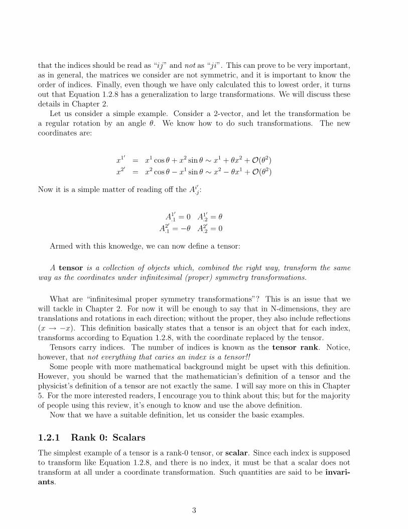
The simplest example of a tensor is a rank-0 tensor, or scalar. Since each index is supposedto transform like Equation 1.2.8, and there is no index, it must be that a scalar does nottransform at all under a coordinate transformation. Such quantities are said to be invari-ants.

3

Notice that an element of a vector, such as x1, is not a scalar, as it does transformnontrivially under Equation 1.2.8.

We will see that the most common example of a scalar is the length of a vector:

s2 =N∑i=1

x2i ≡

N∑i=1

xixi (1.2.9)

Exercise: Prove s is an invariant quantity under translations and rotations. See Section1.3 for details.

1.2.2 Rank 1: Vectors

The next type of tensor is rank-1, or vector. This is a tensor with only one index. Themost obvious example of a vector is the coordinates themselves, which by definition satisfyEquation 1.2.8. There are other examples as well. Some common examples of vectors thatappear in physics are the momentum vector ~p, the electric field ~E, and force ~F . There aremany others.

1.2.3 The General Case

It is a relatively straightforward project to extend the notion of a rank-1 tensor to any rank:just keep going! For example, a rank-2 tensor is an object with two indices (T ij) whichtransforms the following way:

T i′j′ =

N∑k,l=1

Ai′

.kAj′

.l Tkl (1.2.10)

An example of a rank-2 tensor is the moment of intertia from classical rigid-body mechanics.A tensor of rank-3 would have three A’s in the transformation law, etc. Thus we can definetensors of any rank by insisting that they obey the proper transformation law in each index.

1.3 Upstairs, Downstairs: Contravariant vs Covariant

We have put a great deal of emphasis on whether indices belong as superscripts or as sub-scripts. In Euclidean space, where we are all used to working, the difference is less important(although see below), but in general, the difference is huge. Now we will make this quanti-tative. For simplicity, I’ll only consider rank-1 tensors (1 index), but the generalization isvery straightforward.

Recall that we defined a vector as an object which transformed according to Equation1.2.8. There the index was a superscript. We will call vectors of that form contravariantvectors. Now we want to define a vector with an index as a subscript, and we will do itusing Equation 1.2.9.

In any reasonable world, the length of a vector should have nothing to do with thecoordinate system you are using (the magnitude of a vector does not depend on the location

4

of the origin, for example). So we will define a vector with a lower index as an object whichleaves the length invariant:

N∑i=1

xi′xi′ = s2 =

N∑i′=1

(N∑k=1

Ai′

.kxk)(

N∑l=1

xlBl.i′) =

N∑k,l=1

[N∑i′=1

Bl.i′A

i′

.k

]xkxl (1.3.11)

where Bl.i′ is the matrix that defines how this new type of vector is supposed to transform.

Notice that if the left and right side of this expression are supposed to be equal, we have aconstraint on the quantity in brackets:

N∑i′=1

Bl.i′A

i′

.k = δlk (1.3.12)

where δlk is the Kroneker Delta: +1 if k = l, 0 otherwise. In matrix notation, this reads:

BA = 1⇒ B = A−1 (1.3.13)

So we know what B must be. Reading off the inverse is quite easy, by comparing withthe definition of A in Equation 1.2.7:

Bj.i′ =

∂xj

∂xi′≡ Aj.i′ (1.3.14)

The last step just came from noting that B is identical to A with the indices switched. Sowe have defined a new quantity, which we will call a covariant vector. It is just like acontravariant vector except that it transforms in exactly the oposite way:

xi′ =N∑j=1

xjAj.i′ (1.3.15)

There is one more very important point to notice about the contravariant and covariantvectors. Recall from Equation 1.1.3 that the length of a vector can be written as:

s2 =N∑

i,j=1

gijxixj

But we also wrote another equation for s2 in Equation 1.3.11 when we started definingthe covariant vector. By comparing these two equations, we can conclude a very usefulrelationship between covariant and contravariant vectors:

5

1

2

x

Figure 1.1: A graph showing the difference between covariant and contravariant coordinates.

xi =N∑j=1

gijxj (1.3.16)

xj =N∑k=1

gjkxk (1.3.17)

N∑j=1

gijgjk = δki (1.3.18)

So we have found that the metric takes contravariant vectors to covariant vectors andvice versa, and in doing so we have found that the inverse of the metric with lower indicesis the metric with upper indices. This is a very important identity, and will be used manytimes.

When working in an orthonormal flat-space coordinate system (so gij = δij), the differencebetween covariant and contravariant is negligible. We will see in Chapters 3 and 4 someexamples of where the difference begins to appear. But even now I can show you a simplenontrivial example. Consider a cartesian-like coordinate system, but now let the coordinateaxes cross at an angle of 60 deg (see Figure 1.1). Now the metric is no longer proportionalto the Kroneker delta (compare this to Equation (1.1.4), and so there will be a differencebetween covariant and contravariant coordinates. You can see that explicitly in the figureabove, where the same point has x1 < x2, but x1 > x2. So we find that covariant andcontravariant are the same only in orthonormal cartesian coordinates! In the more generalcase, even in flat space, the difference is important.

As another example, consider polar coordinates (r, θ). Even though polar coordinatesdescribe the flat plane, they are not orthonormal coordinates. Specifically, if xi = (r, θ), thenit is true that xi = (r, r2θ), so here is another example of how covariant and contravariantmakes a difference.

6

1.4 Mixed Tensors

We have talked about covariant and contravariant tensors. However, by now it should beclear that we need not stop there. We can construct a tensor that is covariant in one indexand contravariant in another. Such a tensor would be expected to transform as follows:

T i′

.j′ =N∑

k,l=1

Ai′

.kAl.j′T

k.l (1.4.19)

Such objects are known as mixed tensors. By now you should be able to construct a tensorof any character with as many indices as you wish. Generally, a tensor with n upper indicesand l lower indices is called a (n, l) tensor.

1.5 Einstein Notation

The last thing to notice from all the equations so far is that every time we have an indexthat is repeated as a superscript and a subscript, we are summing over that index. This isnot a coincidence. In fact, it is generally true that anytime two indices repeat in a monomial,they are summed over. So let us introduce a new convention:

Anytime an index appears twice (once upstairs, once downstairs) it is to be summed over,unless specifically stated otherwise.

This is known as Einstein notation, and will prove very useful in keeping the expressionssimple. It will also provide a quick check: if you get an index repeating, but both subscriptsor superscripts, chances are you made a mistake somewhere.

1.5.1 Another Shortcut

There is another very useful shortcut when writing down derivatives:

f(x),i = ∂if(x) ≡ ∂f

∂xi(1.5.20)

Notice that the derivative with respect to contravariant-x is covariant; the proof of thisfollows from the chain rule and Equation (1.2.6) This is very important, and is made muchmore explicit in this notation. I will also often use the shortand:

∂2 = ∂i∂i = ∇2 (1.5.21)

This is just the Laplacian in arbitrary dimensions1. It is not hard to show that it is a scalaroperator. In other words, for any scalar φ(x), ∂2φ(x) is also a scalar.

1In Minkowski space, where most of this is relevant for physics, there is an extra minus sign, so ∂2 = =∂2

∂t2 −∇2,which is just the D’Alembertian (wave equation) operator. I will cover this more in Chapter 3; in

this chapter, we will stick to the usual Euclidean space.

7

1.6 Some Special Tensors

1.6.1 Kroneker Delta

We have already seen the Kroneker Delta in action, but it might be useful to quickly sumup its properties here. This object is a tensor which always carries two indices. It is equalto +1 whenever the two indices are equal, and it is 0 whenever they are not. Notice that inmatrix form, the Kroneker Delta is nothing more than the unit matrix in N dimensions:

[δij] =

1 0 · · ·0 1 · · ·...

.... . .

Notice that the Kroneker delta is naturally a (1, 1) tensor.

1.6.2 Levi-Civita Symbol

The Levi-Civita symbol (ε) is much more confusing than the Kroneker Delta, and is thesource of much confusion among students who have never seen it before. Before we dive intoits properties, let me just mention that no matter how complicated the Levi-Civita Symbolis, life would be close to unbearable if it wasn’t there! In fact, it wasn’t until Levi-Civitapublished his work on tensor analysis that Albert Einstein was able to complete his work onGeneral Relativity- it’s that useful!

Recall what it means for a tensor to have a symmetry (for now, let’s only consider arank-2 tensor, but the arguments generalize). A tensor Tij is said to be symmetric ifTij = Tji and antisymmetric if Tij = −Tji. Notice that an antisymmetric tensor cannothave diagonal elements, because we have the equation Tii = −Tii ⇒ Tii = 0 (no sum). Ingeneral, tensors will not have either of these properties; but in many cases, you might wantto construct a tensor that has a symmetry of one form or another. This is where the powerof the Levi-Civita symbol comes into play. Let us start with a definition:

The Levi-Civita symbol in N dimensions is a tensor with N indices such that it equals +1if the indices are an even permutation and −1 if the indices are an odd permutation,and zero otherwise.

We will talk about permutations in more detail in a little while. For now we will simplysay ε12···N = +1 if all the numbers are in ascending order. The Levi-Civita symbol is acompletely antisymmetric tensor, i.e.: whenever you switch two adjacent indices you gain aminus sign. This means that whenever you have two indices repeating, it must be zero (seethe above talk on antisymmetric tensors).

That was a lot of words; let’s do some concrete examples. We will consider the threemost important cases (N=2,3,4). Notice that for N=1, the Levi-Civita symbol is rather silly!

8

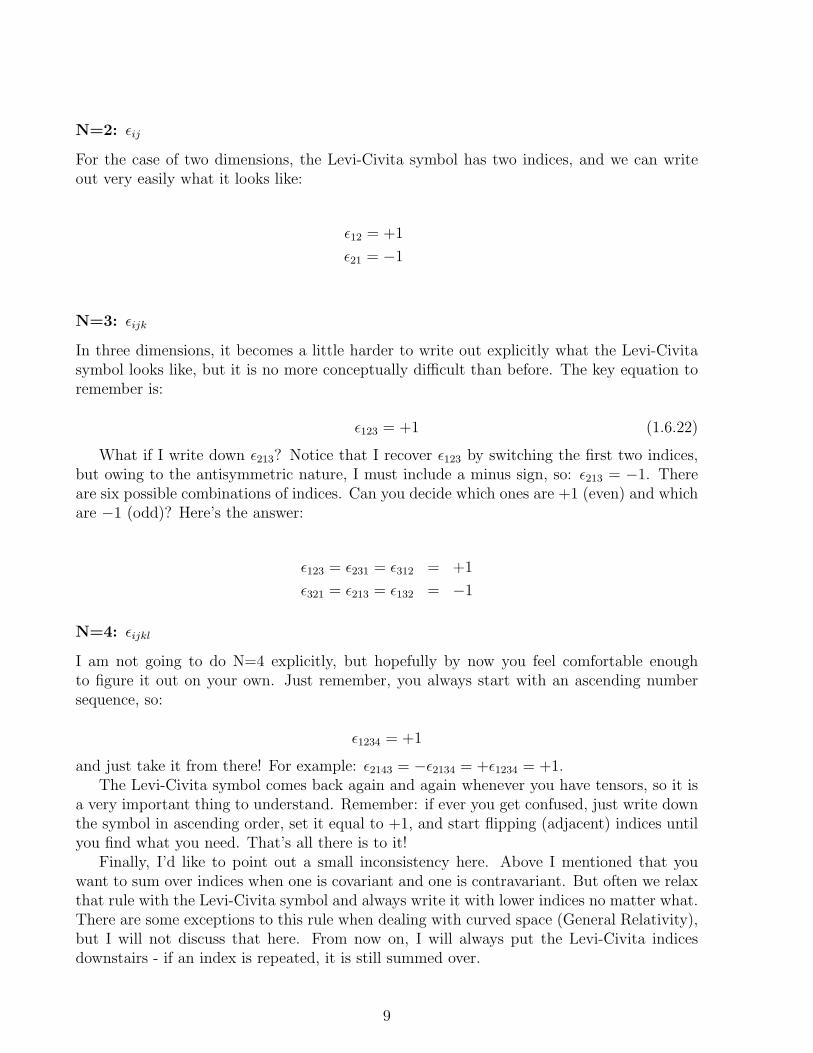
N=2: εij

For the case of two dimensions, the Levi-Civita symbol has two indices, and we can writeout very easily what it looks like:

ε12 = +1

ε21 = −1

N=3: εijk

In three dimensions, it becomes a little harder to write out explicitly what the Levi-Civitasymbol looks like, but it is no more conceptually difficult than before. The key equation toremember is:

ε123 = +1 (1.6.22)

What if I write down ε213? Notice that I recover ε123 by switching the first two indices,but owing to the antisymmetric nature, I must include a minus sign, so: ε213 = −1. Thereare six possible combinations of indices. Can you decide which ones are +1 (even) and whichare −1 (odd)? Here’s the answer:

ε123 = ε231 = ε312 = +1

ε321 = ε213 = ε132 = −1

N=4: εijkl

I am not going to do N=4 explicitly, but hopefully by now you feel comfortable enoughto figure it out on your own. Just remember, you always start with an ascending numbersequence, so:

ε1234 = +1

and just take it from there! For example: ε2143 = −ε2134 = +ε1234 = +1.The Levi-Civita symbol comes back again and again whenever you have tensors, so it is

a very important thing to understand. Remember: if ever you get confused, just write downthe symbol in ascending order, set it equal to +1, and start flipping (adjacent) indices untilyou find what you need. That’s all there is to it!

Finally, I’d like to point out a small inconsistency here. Above I mentioned that youwant to sum over indices when one is covariant and one is contravariant. But often we relaxthat rule with the Levi-Civita symbol and always write it with lower indices no matter what.There are some exceptions to this rule when dealing with curved space (General Relativity),but I will not discuss that here. From now on, I will always put the Levi-Civita indicesdownstairs - if an index is repeated, it is still summed over.

9

1.6.3 Using the Levi-Civita Symbol

Useful Relations

When performing manipulations using the Levi-Civita symbol, you often come across prod-ucts and contractions of indices. There are two useful formulas that are good to remember:

εijkεijl = 2δkl (1.6.23)

εijkεilm = δjklm ≡ δljδmk − δlkδmj (1.6.24)

Exercise: Prove these formulas.

Cross Products

Later, in Chapter 5, we will discuss how to take a generalized cross-product in n-dimensions.For now, recall that a cross product only makes sense in three dimensions. There is abeautiful formula for the cross product using the Levi-Civita symbol:

( ~A× ~B)i = εijkAjBk (1.6.25)

Using this equation, and Equations (1.6.23) and (1.6.24), you can derive all the vectoridentities on the cover of Jackson, such as the double cross product. Try a few to get thehang of it. That’s a sure-fire way to be sure you understand index manipulations.

As an example, let’s prove a differential identity:

∇× (∇×A) = εijk∂jεklm∂lAm = εkijεklm∂j∂lAm

= [δilδjm − δimδjl]∂j∂lAm = ∂i∂mAm − ∂2Ai = ∇(∇ ·A)−∇2A

Exercise: Prove that you can interchange dot and cross products: A ·B×C = A×B ·C.

1.7 Permutations

A permutation is just a shuffling of objects. Rigorously, consider a set of objects (calledS) and consider an automorphism σ : S → S (one-to-one and onto function). Then σ is apermutation. It takes an element of S and sends it uniquely to another element (possiblythe same element) of S.

One can see very easily that the set of all permutations of a (finite) set S is a groupwith multiplication defined as function composition. We will talk more about groups in thenext chapter. If the set S has n elements, this group of permutations is denoted Sn, and isoften called the Symmetric group. It has n! elements. The proof of this is straightforwardapplication of group and number theory, and I will not discuss it here.

The theory of symmetric groups is truly deep and of fundamental importance in math-ematics, but it also has much application in other branches of science as well. For thatreason, let me give a very brief overview of the theory. For more information, I recomendyour favorite abstract algebra textbook.

10

Specific permutations are usually written as a row of numbers. It is certainly true (andis rigorously provable for the anal retentive!) that any finite set of order n (i.e.: with nelements) can be represented by the set of natural numbers between 1 and n. Then WLOG2

we can always represent our set S in this way. Then a permutation might look like this:

σ = (1234)

This permutation sends 1 7→ 2,2 7→ 3,3 7→ 4,4 7→ 1. This is in general how it always works.If our set has four elements in it, then this permutation touches all of them. If it has morethan four elements, it leaves any others alone (for example, 5 7→ 5).

Working in S5 for the moment, we can write down the product of two permutations bycomposition. Recall that composition of functions always goes rightmost function first. Thisis very important here, since the multiplication of permutations is almost never commutative!Let’s see an example:

(1234)(1532) = (154)

Where did this come from? Start with the first number in the rightmost permutation (1).Then ask, what does 1 go to? Answer: 5. Now plug 5 into the secondmost right transposition,where 5 goes to 5. Net result: 1 7→ 5. Now repeat the same proceedure on 5 to get 5 7→ 4,and so on until you have completed the cycle (quick check: does 2 7→ 2,3 7→ 3?). Multiplyingthree permutations is just as simple, but requires three steps instead of two.

A permutation of one number is trivial, so we don’t worry about it. A transpositionis a permutation of two numbers. For example: (12) sends 1 7→ 2,2 7→ 1. It is a trulyamazing theorem in group theory that any permutation (no matter what it is) can be writtenas a product of transpositions. Furthermore, this decomposition is unique up to trivialpermutations. Can you write down the decomposition of the above product3?

Armed with that knowledge, we make a definition:

Definition: If a permutation can be written as a product of an even number of trans-positions, it is called an even permutation. If it can be written as an odd number ofperumtations, it is called an odd permutation. We define the signature of a permutationin the following way:

sgn(σ) =

+1 σ even−1 σ odd

(1.7.26)

It is pretty obvious that we have the following relationships:

(even)(even) = (even)(odd)(odd) = (even)

(odd)(even) = (even)(odd) = (odd)

2Without Loss Of Generality3Answer: (15)(45). Notice that this is not the same as (45)(15).

11

What this tells us is that the set of even permutations is closed, and hense forms asubgroup, called the Alternating Subgroup (denoted An) of order 1

2n!. Again, I omit

details of the proof that this is indeed a subgroup, although it’s pretty easy. Notice that theodd elements do not have this property. The alternating subgroup is a very powerful tool inmathematics.

For an application of permutations, a good place to look is index manipulation (hencewhy I put it in this chapter!). Sometimes, you might want to sum over all combinations ofindices. For example, the general formula for the determinant of an n × n matrix can bewritten as:

detA =∑σ∈Sn

sgn(σ)a1σ(1)a2σ(2) · · · anσ(n) (1.7.27)

1.8 Constructing and Manipulating Tensors

To finish this chapter, I will review a few more manipulations that provide ways to constructtensors from other tensors.

1.8.1 Constructing Tensors

Consider two tensors of rank k (K) and l (L) respectively. We want to construct a new tensor(T) from these two tensors. There are three immediate ways to do it:

1. Inner Product: We can contract one of the indices from K and one from L to forma tensor T of rank k + l− 2. For example, if K is rank 2 and L is rank 3, then we cancontract, say, the first index of both of them to form T with rank 3:

Tµνρ = Kα.µLανρ

We could construct other tensors as well if we wished by contracting other indices.We could also use the metric tensor or the Levi-Civita tensor if we wished to formsymmetric or antisymmetric combinations of tensors. For example, if A,B are vectorsin 4 dimensions:

Tµν = εµνρσAρBσ ⇒ T12 = A3B4 − A4B3, etc.

2. Outer Product: We can always construct a tensor by combining two tensors withoutcontracting any indices. For example, if A and B are vectors, we can construct: Tij =AiBj. Because we are using a Cartesian coordinate system, we call tensors of this formCartesian Tensors. When combining two vectors in this way, we say that we haveconstructed a Dyadic.

3. Symmetrization: Consider the outer product of two vectors AiBj. Then we can forcethe tensor to be symmetric (or antisymmetric) in its indices by construction:

12

A(iBj) ≡1

2(AiBj + AjBi) (1.8.28)

A[iBj] ≡1

2(AiBj − AjBi) (1.8.29)

Circular brackets about indices mean symmetric combinations, and square bracketsabout indices mean antisymmetric combinations. You can do this to as many indicesas you want in an outer product (for n indices, replace 1

2→ 1

n!).

Dyadics provide a good example of how combining tensors can be more involved than itfirst seems. Consider the dyadic we have just constructed. Then we can write it down in afancy way by adding and subtracting terms:

Tij =1

N(T kk )δij +

1

2(Tij − Tji) + [

1

2(Tij + Tji)−

1

N(T kk )δij] (1.8.30)

N is the dimension of A and B, and the sum over k in the first and last terms is impliedby Einstein notation. Notice that I have not changed the tensor at all, because any term Iadded I also subtracted. However, I have decomposed the tensor into three different pieces.The first piece is just a scalar (times the identity matrix), and therefore is invariant underrotations. The next term is an antisymmtric tensor, and (in 3D) can be written as a (pseudo)vector- it’s a cross product (see Equation (1.6.25)). Finally the third piece is a symmetric,traceless tensor.

Let’s discuss the matter concretely by letting N = 3 and counting degrees of freedom. IfA and B are 3-vectors, then Tij has 3 × 3 = 9 components. Of the three pieces, the first isa scalar (1), the second is a 3-vector (3) and the third is a rank-2 symmetric tensor (6) thatis traceless (-1); so we have decomposed the tensor according to the following prescription:

3⊗ 3 = 1⊕ 3⊕ 5

We say that the dyatic form Tij is a reducible Cartesian tensor, and it reduces into 3irreducible spherical tensors, each of rank 0, 1 and 2 respectively.

1.8.2 Kroneker Products and Sums

With that introduction, we can talk about Kroneker products and sums. A Kronekerproduct is simply an outer product of two tensors of lesser rank. A dyatic is a perfectexample of a Kroneker Product. Writing it out in a matrix, we have (for A,B rank-1 tensorsin 3 dimensions):

T = A⊗B =

A1B1 A1B2 A1B3

A2B1 A2B2 A2B3

A3B1 A3B2 A3B3

(1.8.31)

A Kroneker sum is the concatinated sum of matrices. You can write the Kroneker sumin matrix form using a block-diagonal matrix:

13

T = C⊕D⊕ E =

C 0 00 D 00 0 E

(1.8.32)

where C is an m×m matrix, D is an n×n matrix, E is an l× l matrix,and “0” is just fillingin any left over entries with a zero. Notice that the final matrix is an (m+n+ l)×(m+n+ l)matrix.

At this point, we can rewrite our equation for the dyadic:

A⊗B ∼ C⊕D⊕ E (1.8.33)

where A⊗B is a 3× 3 matrix, C is 1× 1, D is 3× 3 and E is 5× 5. Notice that the matrixdimensions are not the same on both sides of the equation - these are not the same matrix!However, they each have the same number of independent quantities, and both representthe same tensor T. For this reason, the study of finding different dimensional matrices forT goes under the heading of representation theory. It is a very active part of modernalgebraic research, and is very useful in many areas of science.

Why would one ever want to do this? The answer is that when working with dyadics inpractice, very often one is only interested in the part of the tensor that transforms the sameway. Notice that when you rotate T, you never mix terms between C, D and E. This kind ofrelationship is by no means as obvious when written in its Cartesian form. For that reason,it is often very useful to work with the separate spherical tensors rather than with the entireCartesian tensor. The best example is in Quantum Mechanics, when you are talking aboutangular momentum. See Sakurai for more details.

14

Chapter 2

Transformations and Symmetries

2.1 Symmetries and Groups

Here we will discuss some properties of groups in general that you need to know. Thenwe will progress to discuss a very special and important kind of group, called a Lie Group.Finally we will look at some examples.

• Definition: A group G is a set with an operator called multiplication that obeys fouraxioms: Closure (g1, g2 ∈ G⇒ g1g2 ∈ G), Associative((g1g2)g3 = g1(g2g3)), an identity(generically called e such that ge = eg = g) and inverses (g has inverse g−1 such thatgg−1 = g−1g = e). If the group is commutative (g1g2 = g2g1), it is said to be anAbelian group, otherwise it is Non-Abelian.

• Discrete groups represent operations that either do or do not take place. Continuousgroups represent operations that differ infinitesimally from each other.

• Elements in continuous groups can be labeled by a set of continuous parameters. Ifthe set of parameters is finite, the group is said to be a finite group. If the ranges ofthe parameters are closed and bounded, the group is said to be a compact group.

• Definition: A subgroup is a subset of a larger group that is also a group. A subgroupN ⊂ G is a normal subgroup (also called invariant subgroup) if ∀si ∈ N, g−1sig ∈N ∀g ∈ G. In other words, elements of N stay in N after being multiplied by elementsin G. We write N / G. There are several definitions for invariant subgroups, but theyare all equivalent to this one.

• Consider two groups that commute with each other (G,H). Then you can constructthe direct product group in the following way: G × H ≡ (gjhk)|(gjhk)(glhm) =(gjglhkhm). Be careful not to confuse a direct product group with a Kroneker productof tensors.

• Fact: G,H / G×H are invariant subgroups.

• Definition: If a group has no invariant subgroups, it is called a simple group.

15

• Definition: Suppose there is a square n×n matrix M that corresponds to each elementof a group G, where g1g2 = g3 ⇒ M(g1)M(g2) = M(g3) and M(g−1) = [M(g)]−1.Then M is called a representation of the group G, and n is called the dimensionof the representation. If this identification is one-to-one, the representation is called“faithful”. An example of an unfaithful representation is where all elements of a groupG go to 1.

• Definition: A representation is reducible if each matrix can be expressed in block-diagonal form. Using the Kroneker sum notation, we can rephrase this definition:∃A,B such that M = A ⊕ B. A and B are also valid representations of the group.Furthermore, they do not talk to each other (think angular momentum in quantummechanics). If a representation is not reducible, it is said to be irreducible.

• Consider an n-tuple ξa, not necessarely a vector in the sense of Chapter 1. Thenthe group element g inan n−dimensional representation M acts on the vector in thefollowing way:

ξ′

a = M(g).ba ξb

(recall Einstein notation). Since the matrix M must be nonsingular (otherwise there

would be no g−1 and it wouldn’t be a group), ∃ξa such that ξa′

= ξb[M(g)−1].ab . ξ is

called the adjoint of ξ.

• Definition: The smallest (lowest dimension) nontrivial irreducible faithful representa-tion is called the fundamental representation. We will see some examples of thisshortly. Here, the “trivial” representation is the one-dimensional representation.

• Definition: A Lie group is a continuous group that is also a manifold whose mul-tiplication and inverse operations are differentiable. It is named after Sophus Lie,the mathematician who first discovered their properties. This definition is quite amouthful- don’t worry too much about it if you’re not a theorist! Things will becomea lot simpler once we get to some examples. But before that, here are some importantresults you should know:

• Theorem: All compact Lie groups have unitary representations. In other words:M(ε) = eiε

jFj , j = 1, . . . , N , and Fj matrices1. The Fj are called generators. Fromthis we can see that M † = M−1, as long as F † = F , so we require that the generatorsbe Hermitian. Warning: the index on F is not a matrix index - Fj = (Fj)ab.

• Many (though not all) Lie groups have the additional property that detM(ε) = +1∀ε. From the above result, this implies Tr(Fi) = 0; this can be proved with the helpof the very useful fact

detA = eTr logA

This is called the special condition.

1Recall the definition for the exponential of a matrix: eA =∑∞n=0

(A)n

n!

16

• When ε is small, we can expand the exponential to get:

M(ε) = I + iεjFj +O(ε2)

This is exactly the same as an infinitesimal transformation, and so we say that Fjgenerates infinitesimal transformations.

• Theorem: The local structure of any Lie group is completely specified by a set ofcommutation relations among the generators:

[Fi, Fj] = ifijkFk (2.1.1)

(the sum over k is understood). These commutators specify an algebra spanned by thegenerators2, and the fijk are called the structure constants of the Lie group. Theyare the same for any representation of the group.

• Theorem: fijlflkm + fkilfljm + fjklflim = 0. The proof follows from Jacobi’s identity forcommutators.

• In general, the structure constants are antisymmetric in their indices.

• Notice that we can rearrange the above version of the Jacobi identity and use theantisymmetry to rewrite it as:

(fi)jl(fk)lm − (fk)jl(fi)lm = −fikl(fl)jm (2.1.2)

where I have just separated the indices in a convienient way, but nothing more. Thenif I define a matrix with the elements (Fi)jk ≡ −ifijk, I have reproduced Equation(2.1.1). Therefore, this is a valid representaion! It is so important, it is given a specialname - it is called the regular adjoint representation.

• Definition: The rank of a Lie group is the number of simultaneously diagonalizeablegenerators; that is, the number of generators that commute among themselves. Thisset of generators forms a subalgebra called the Cartan Subalgebra. The rank of thegroup is the dimension of this subalgebra.

• Definition: C(n) ≡ fi1j1j2fi2j2j3 · · · finjnj1Fi1Fi2 · · ·Fin are called the Casimir opera-tors notice that all indices are repeated and therefore summed via Einstein conven-sion).

• Casimir operators commute with every generator; hence they must be multiples of theidentity. This means that they represent conserved quantities. It is also true that thenumber of Casimir operators is equal to the rank of the group.

That’s enough general stuff. Let’s look at some very important examples:

2An algebra is a vector space with a vector product, where in this case, the basis of this vector space isthe set of generators (see Chapter 5). This algebra is called a Lie Algebra.

17

2.1.1 SU(2) - Spin

• Consider a complex spinor

ξ =

(ξ1

ξ2

)and the set of all transformations which leave the norm of the spinor invariant; i.e.:

s2 = |ξ1|2 + |ξ2|2

s invariant under all transformations. We will also require detM = 1. From the above,we know that the generators (call them σi) must be linearly independent, traceless,Hermitian 2× 2 matrices. Let us also include a normalization condition:

Tr(σiσj) = 2δij

Then the matrices we need are the Pauli matrices:

σ1 =

(0 11 0

)σ2 =

(0 −ii 0

)σ3 =

(1 00 −1

)(2.1.3)

Then we will chose the group generators to be Fi = 12σi. The group generated by

these matrices is called the Special Unitary group of dimension 2, or SU(2). In thefundamental representation, it is the group of 2×2 unitary matrices of unit determinant.

• Recall from quantum mechanics that the structure constants are simply given by theLevi-Civita tensor:

fijk = εijk

• Only σ3 is diagonal, and therefore the rank of SU(2) is 1. Then there is only oneCasimir operator, and it is given by:

C(2) = F 21 + F 2

2 + F 23

• If we remove the Special condition (unit determinant), then the condition that Trσi = 0no longer need hold. Then there is one more matrix that satisfies all other conditionsand is still linearly independent from the others- the identity matrix:

σ0 =

(1 00 1

)Notice, however that this is invariant:

eiεjFjeiε

0F0e−iεjFj = eiε

0F0 (2.1.4)

Therefore, the group generated by eiε0F0 is an invariant subgroup of the whole group.

We call it U(1). That it is a normal subgroup should not suprise you, since it is truethat eiε

0F0 = (eiε0/2)σ0, which is a number times the identity matrix.

18

• The whole group (without the special) is called U(2). We have found U(1) / U(2),SU(2) / U(2) and we can write:

U(2) = SU(2)× U(1) (2.1.5)

This turns out to be true even in higher dimensional cases:

U(N) = SU(N)× U(1)

• Sumarizing: R = eiθ2

(~n·~σ) is the general form of an element of SU(2) in the fundamentalrepresentation. In this representation, C(2) = 2, as you might expect if you followedthe analogy from spin in quantum mechanics.

• You know from quantum mechanics that there are other representations of spin (withdifferent dimensions) that you can use, depending on what you want to describe - thischange in representation is nothing more than calculating Clebsch-Gordon coefficients!

• Example: what if you want to combine two spin-12

particles? Then you know that youget (3) spin-1 states and (1) spin-0 state. We can rewrite this in terms of representationtheory: we’ll call the fundamental representation 2, since it is two-dimensional. Thespin-1 is three dimensional and the spin-0 is one dimensional, so we denote them by 3and 1 respecitively. Then we can write the equation:

2⊗ 2 = 3⊕ 1 (2.1.6)

(Notice once again that the left hand side is a 2× 2 matrix while the right hand sideis a 4 × 4 matrix, but both sides only have four independent components). Equation(2.1.6) is just saying that combining two spin-1

2particles gives a spin-1 and a spin-0

state, only using the language of groups. In this language, however, it becomes clearthat the four-dimensional representation is reducible into a three-dimensional and aone-dimensional representation. So all matrix elements can be written as a Kronekersum of these two representations. Believe it or not, you already learned this when youwrote down the angular momentum matrices (recall they are block-diagonal). This alsoshows that you do not need to consider the entire (infinitely huge) angular momentummatrix, but only the invariant subgroup that is relevant to the problem. In otherwords, the spin-1 and spin-0 do not talk to each other!

2.1.2 SO(3,1) - Lorentz (Poincare) Group

Much of this information is in Jackson, Chapter 11, but good ol’ JD doesn’t always makethings very clear, so let me try to summarize.

• The Poincare Group is the set of all transformations that leave the metric of flatspace-time invariant (see Chapter 4). The metric in Minkowski (flat) space is givenby:

ds2 = c2dt2 − dr2

19

• Intuitively we know that this metric is invariant under parity (space reversal), timereversal, spacial rotations, space and time translations and Lorentz transformations.Then we know that these operations should be represented in the Poincare group.

• Ignore translations for now. You can prove to yourself that the matrices that representthe remaining operators must be orthogonal (OT = O−1); the group of n×n orthogonalmatrices is usually denoted by O(n). In this case, n = 4; however, there is a minus signin the metric that changes things somewhat. Since three components have one sign,and one component has another, we usually denote this group as O(3,1), and we callit the Lorentz group.

• The transformations we are interested in are the proper orthochronous transformations-i.e.: the ones that keep causality and parity preserved. This is accomplished by im-posing the “special” condition (detO = +1). However, this is not enough: althoughthis forbids parity and time-reversal, it does not forbid their product (prove this!). Sowe consider the Proper Orthochronous Lorentz Group, or SO(3, 1)+, where the“orthochronous” condition (subscript “+” sign) is satisfied by insisting the the (00)component of any transformation is always positive; that along with the special condi-tion is enough to isolate the desired subgroup. As this is quite a mouthful, we usuallyjust refer to SO(3,1) as the Lorentz group, even though it’s really only a subgroup.

• We can now go back to Chapter 1 and rephrase the definition of a tensor in flat space-time as an object that transforms under the same way as the coordinates under anelement of the Lorentz group.

• The Lorentz group has six degrees of freedom (six parameters, six generators). For aproof, see Jackson. We can interpret these six parameters as three spacial rotations andthree boosts, one about each direction. We will denote the rotation matrix generatorsas Si, and the boost generators as Ki, where i = 1, 2, 3. These matrices are:

S1 =

0 0 0 00 0 0 00 0 0 −10 0 1 0

S2 =

0 0 0 00 0 0 10 0 0 00 −1 0 0

S3 =

0 0 0 00 0 −1 00 1 0 00 0 0 0

K1 =

0 1 0 01 0 0 00 0 0 00 0 0 0

K2 =

0 0 1 00 0 0 01 0 0 00 0 0 0

K3 =

0 0 0 10 0 0 00 0 0 01 0 0 0

• In general, we can write any element of the Lorentz group as e−[θ·S+η·K], where θ are the

three rotation angles, and η are the three boost parameters, called the rapidity. Youshould check to see that this exponential does in fact give you a rotation or Lorentztransformation when chosing the proper variables. See Jackson for the most generaltransformation.

20

• The boost velocity is related to the rapidity by the equation:

βi ≡ tanh ηi (2.1.7)

• Exercise: what is the matrix corresponding to a boost in the x-direction? Answer:cosh η sinh η 0 0sinh η cosh η 0 0

0 0 1 00 0 0 1

=

γ γβ 0 0γβ γ 0 00 0 1 00 0 0 1

where γ = (1− β2)−1/2. This is what you’re used to seeing in Griffiths!

• Notice that you can always boost along a single direction by combining rotations withthe boosts. This is certainly legal by the nature of groups!

• The angles are bounded: 0 ≤ θ ≤ 2π, but the rapidities are not: 0 ≤ η < ∞. TheLorentz group is not a compact group! And therefore it does not have faithful unitaryrepresentations. This is a big problem in Quantum Mechanics and comes into playwhen trying to quantize gravity.

• The Lorentz algebra is specified by the commutation relations:

[Si, Sj] = εijkSk

[Si, Kj] = εijkKk

[Ki, Kj] = −εijkSk

Some points to notice about these commutation relations:

1. The rotation generators form a closed subalgebra (and hense generate a closedsubgroup) – it is simply the set of all rotations, SO(3). It is not a normal subgroup,however, becuase of the second commutator.

2. A rotation followed by a boost is a boost, as I mentioned above.

3. Two boosts in diferent directions correspond to a rotation about the third direc-tion.

4. The minus sign in the last commutator is what makes this group the noncompactSO(3,1), as opposed to the compact SO(4), which has a + sign.

• Notice that you could have constructed the generators for the Lorentz group in a verysimilar way to how you construct generators of the regular rotation group (angularmomentum):

Jµν = x ∧ p = i~(xµ∂ν − xν∂µ) (2.1.8)

21

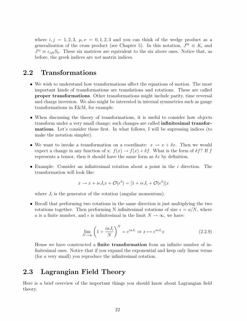
where i, j = 1, 2, 3, µ, ν = 0, 1, 2, 3 and you can think of the wedge product as ageneralization of the cross product (see Chapter 5). In this notation, J0i ≡ Ki andJ ij ≡ εijkSk. These six matrices are equivalent to the six above ones. Notice that, asbefore, the greek indices are not matrix indices.

2.2 Transformations

• We wish to understand how transformations affect the equations of motion. The mostimportant kinds of transformations are translations and rotations. These are calledproper transformations. Other transformations might include parity, time reversaland charge inversion. We also might be interested in internal symmetries such as gaugetransformations in E&M, for example.

• When discussing the theory of transformations, it is useful to consider how objectstransform under a very small change; such changes are called infinitesimal transfor-mations. Let’s consider these first. In what follows, I will be supressing indices (tomake the notation simpler).

• We want to invoke a transformation on a coordinate: x → x + δx. Then we wouldexpect a change in any function of x: f(x)→ f(x) + δf . What is the form of δf? If frepresents a tensor, then it should have the same form as δx by definition.

• Example: Consider an infinitesimal rotation about a point in the i direction. Thetransformation will look like:

x→ x+ iεJix+O(ε2) = [1 + iεJi +O(ε2)]x

where Ji is the generator of the rotation (angular momentum).

• Recall that performing two rotations in the same direction is just multiplying the tworotations together. Then performing N infinitesimal rotations of size ε = a/N , wherea is a finite number, and ε is infinitesimal in the limit N →∞, we have:

limN→∞

(1 +

iaJiN

)N= eiaJi ⇒ x 7→ eiaJix (2.2.9)

Hense we have constructed a finite transformation from an infinite number of in-finitesimal ones. Notice that if you expand the exponential and keep only linear terms(for a very small) you reproduce the infinitesimal rotation.

2.3 Lagrangian Field Theory

Here is a brief overview of the important things you should know about Lagrangian fieldtheory.

22

• Recall in Lagrangian mechanics, you define a Lagrangian L(q(t), q(t)) and an actionS =

∫Ldt. Now we wish to decribe a Lagrangian density L(φ(x), ∂µφ(x)) where

L =∫Ld3x, and φ is a field which is a funtion of spacetime. The action can be written

as S =∫Ld4x. The action completely specifies the theory.

• The equations of motion can now be found, just as before by the condition δS = 0.This yields the new Euler-Lagrange equations:

∂L∂φ− ∂µ

(∂L∂φ,µ

)= 0 (2.3.10)

Notice that there is the sum over the index µ, following Einstein notation.

• Example: L = 12∂µφ∂

µφ − 12m2φ2 is the Lagrangian for a scalar field (Klein-Gordon

field in relativistic quantum mechanics). Can you find the equations of motion? Here’sthe answer:

(∂2 +m2)φ = 0

• Just as in classical mechanics, we can also go to the Hamiltonian formalism, by defininga momentum density:

π ≡ ∂L∂φ

where φ ≡ ∂0φ and perform the Legendre transformation:

H(φ(x), π(x)) = π(x)φ(x)− L ⇒ H =

∫d3xH (2.3.11)

• Notice that L is covariant, but H is not, since time becomes a special parameter viathe momentum density. This is why we often prefer to use the Lagrangian formalismwhenever working with relativistic mechanics. Nevertheless, this formalism is stillgenerally useful since H is related to the energy in the field.

2.4 Noether’s Theorem

A theory is said to be symmetric with respect to a transformation whenever the action doesn’tchange under that transformation. This implies that the Lagrangian can only change up toa total divergence (via Gauss’s Theorem). To see this, notice that if the Lagrangian changesby a total divergence, we have:

S′=

∫Ld4x+

∫∂µJ µd4x = S +

∫dΣµJ µ

where the last surface integral is an integral over a surface at infinity. In order for quantitieslike energy to be finite, we often require that fields and their derivatives vanish on such a

23

surface. Thi implies that the above surface integral vanishes (or at least doesn’t contributeto the Equations of Motion3). Thus we have

Noether’s Theorem: For every symmetry in the theory, there corresponds a conservedcurrent, and vice versa.

Proof: I will prove Noether’s theorem for a scalar field, but it is true in general for anytype of field. Let’s consider the general transformation that acts on the field according to:

φ→ φ+ αδφ

where α is a constant infinitesimal parameter4. Then if we insist this transformation leavethe action invariant, the previous argument says that the Lagrangian can only change by atotal divergence:

L → L+ α∂µJ µ

Let’s calculate the change in L explicitly:

αδL =∂L∂φ

(αδφ) +∂L∂φ,µ

∂µ(αδφ)

= α∂µ

(∂L∂φ,µ

δφ

)+ α

[∂L∂φ−(∂L∂φ,µ

),µ

]δφ

= α∂µJ µ

To get line 1 from line 2, use the product rule. The term in brackets is zero by Equation(2.3.10), leaving only the total divergence. Then we can combine terms to get:

jµ ≡(∂L∂φ,µ

δφ

)− J µ ⇒ ∂µj

µ = 0 (2.4.12)

hense jµ is a conserverd current, which is precicely what we wanted to show. QED.

Notice that we could also write Noether’s theorem by saying that for every symmetry ofthe theory, there is a “charge” which is conserved:

Q ≡∫j0d3x⇒ dQ

dt= 0

There are many applications of this theorem. You can prove that isotropy of space (rota-tional invariance) implies angular momentum conservation, homogeneity of space (transla-tional invariance) implies linear momentum conservation, time translation invariance implies

3Sometimes this integral does not vanish, and this leads to nontrivial “topological” effects. But this isadvanced stuff, and well beyond the scope of this review. So for now let’s just assume that the surfaceintegral is irrelevant, as it often is in practice.

4This theorem also holds for nonconstant α - I leave the proof to you.

24

energy conservation, etc. You can also consider more exotic internal symmetries; for example,gauge invariance in electrodynamics implies electric charge conservation.

25

Chapter 3

Geometry I: Flat Space

The most important aspect of geometry is the notion of distance. What does it mean for twopoints in a space to be “close” to each other? This notion is what makes geometry distinctfrom topology and other areas of abstract mathematics. In this chapter, I want to definesome important quantities that appear again and again in geometric descriptions of physics,and give some examples.

In this chapter we will always be working in flat space (no curvature). In the next chapter,we will introduce curvature and see how it affects our results.

3.1 THE Tensor: gµν

• Like transformations, we can define distance infinitesimally and work our way up fromthere. Consider two points in space that are separated by infinitesimal distances dx,dy and dz. Then the total displacement (or metric) is given by the triangle rule ofmetric spaces (a.k.a. the Pythagorean theorem):

ds2 = dx2 + dy2 + dz2 ≡ gµνdxµdxν

Here, gµν = δµν .

• Definition: gµν is called the metric tensor or the first fundamental form. Knowingthe form of gµν for any set of coordinates let’s you know how to measure distances.The metric tensor is given by Equation (1.1.4), but in this chapter we will often cheat,since sometimes we already know what ds2 is. But when faced with trying to calculatethe metric in general, usually you have to resort to Equation (1.1.4).

• WARNING: Unlike the usual inner product notation, we never write ds2 = gµνdxµdxν .The dx’s always have upper indices1.

• In Cartesian coordinates, the metric tensor is simply the identity matrix, but in general,it could be off-diagonal, or even be a function of the coordinates.

1This is because dxµ forms a basis for the covectors (1-forms); see Chapter 5. Compare this to thebasis vectors of Chapter 1 ~ei which always came with lower indices, so that

⟨dxi, ~ej

⟩= δij . Notice that

the indices work out exactly as they should for the Kroneker delta - this is, once again, not a coincidence!

26

3.1.1 Curvilinear Coordinates

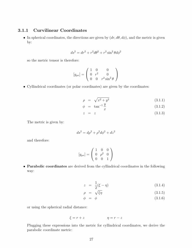
• In spherical coordinates, the directions are given by (dr, dθ, dφ), and the metric is givenby:

ds2 = dr2 + r2dθ2 + r2 sin2 θdφ2

so the metric tensor is therefore:

[gµν ] =

1 0 00 r2 00 0 r2 sin2 θ

• Cyllindrical coordinates (or polar coordinates) are given by the coordinates:

ρ =√x2 + y2 (3.1.1)

φ = tan−1 y

x(3.1.2)

z = z (3.1.3)

The metric is given by:

ds2 = dρ2 + ρ2dφ2 + dz2

and therefore:

[gµν ] =

1 0 00 ρ2 00 0 1

• Parabolic coordinates are derived from the cyllindrical coordinates in the following

way:

z =1

2(ξ − η) (3.1.4)

ρ =√ξη (3.1.5)

φ = φ (3.1.6)

or using the spherical radial distance:

ξ = r + z η = r − z

Plugging these expressions into the metric for cyllindrical coordinates, we derive theparabolic coordinate metric:

27

ds2 =1

4

[(1 +

η

ξ

)dξ2 +

(1 +

ξ

η

)dη2

]+ ξηdφ2

therefore:

[gµν ] =

14

(1 + η

ξ

)0 0

0 14

(1 + ξ

η

)0

0 0 ξη

Parabolic coordinates describe families of concentric paraboloids symmetric about thez-axis. They are very useful in problems with the appropriate symmetry, such asparabolic mirrors.

• As you might have guessed, there are also hyperbolic coordinates and elliptical coor-dinates, but I won’t get into those here. There are even more complicated coordinatesystems that are useful (toroidal coordinates, etc).

3.2 Differential Volumes and the Laplacian

3.2.1 Jacobians

• If you transform your coordinates, you will modify your differential volume element bya factor called the Jacobian:

yα = yα(xβ)⇒ dnx = J dny

where in general, J = det(∂xa

∂yµ

)• To find the general Jacobian, let us consider a transformation from Cartesian coordi-

nates (xa) to general coordinates (yµ) and ask how the metric transforms. Remember-ing that the metric is a (0, 2) tensor and gab = δab we have:

gµν = δab∂xa

∂yµ∂xb

∂yν(3.2.7)

Now take the determinant of both sides, and defining g ≡ det(gµν) we find that J =√g, so in general:

dnx =√gdny

.

28

3.2.2 Veilbeins - a Prelude to Curvature

I will talk about curvature in the next chapter, but now would be a good time to introducea very useful tool called the vielbein (eµa):

• Consider a point p with coordinates xµ on a manifold (generally a manifold withcurvature, which we’ll talk about next Chapter). At every point p ∈ M , there is a“tangent space” – this is basically the flat plane tangent to the manifold at the pointp. Give coordinates on the tangent plane ξa such that the point p is mapped to theorigin. The key point to notice is that the latin index is for flat space while the greekindex is for curved space.

• Now consider a point p on the manifold, and the tangent space at p. Then thereis a (linear) mapping between the points near the origin of the tangent plane (withcoordinates ξa) to a neighborhood of p on the manifold (with coordinates xµ). Thislinear mapping is given by a matrix called the vielbein:

eµa ≡∂xµ

∂ξa

This allows us to write Equation (3.2.7) as:

gµν = δabeaµebν

So the vielbein is, in some sense, the square root of the metric! In particular, the aboveanalysis shows that the Jacobian is just e, the determinant of the vielbein. There aremany cases in physics where this formalism is very useful2. I won’t mention any of ithere, but at least you have seen it.

3.2.3 Laplacians

• We can find the Laplacian of a scalar field in a very clever way using the Variationalprinciple in electrostatics. For our functional, consider that we wish to minimize theenergy of the system, and in electrostatics, that is (up to constants) the integral of E2.So using our scalar potential, let’s define the energy functional in cartesian coordinates:

W [Φ] =

∫dnx(∇Φ)2

where dnx is the n−dimensional differential volume element.

• We can find the extremum of this functional δW [Φ] = 0 and see what happens. Atfirst, notice that an integration by parts lets you rewrite the integrand as −Φ∇2Φ,and the variation of that is simply −δΦ∇2Φ. Now change coordinates using the aboveprescription and repeat the variation. We set the two expressions equal to each other,

2For example, when spin is involved.

29

since the integral must be the same no matter what coordinate system we use. Thenyou get as a final expression for the Laplacian:

∇2 =1√g∂α[√ggαβ∂β] (3.2.8)

Exercise: Prove this formula. It’s not hard, but it’s good practice.

Notice that ∂µ is covariant, so we require the contravariant gµν - remember that thisis the inverse of the metric, so be careful!

• Notice that this expression is only valid for scalar fields! For vector fields, it is generallymore complicated. To see this, notice that at first, you might assume that ∇2A =(∇2Ai) for each component Ai. In Cartesian coordinates, this is fine. But in curvilinearcoordinates, you must be extra careful. The true definition of the ith vector componentis Ai = A · ~ei, and in curvilinear coordinates, ~ei has spacial dependence, so you haveto take its derivative as well. We will take the derivative of a unit vector and discussits meaning in the next chapter.

• Exercise: Find the Laplacian in several different coordinate systems using Equation(3.2.8). The usual Laplacians are on the cover of Jackson. Can you also find theLaplacian in parabolic coordinates? Here’s the answer:

∇2 =4

ξ + η

[ξ∂2

∂ξ2+

∂

∂ξ+ η

∂2

∂η2+

∂

∂η

]+

1

ξη

∂2

∂φ2

3.3 Euclidean vs Minkowskian Spaces

What is the difference between Euclidean space and Minkowski space? In all the exampleswe have considered so far, we have been in three dimensions, whereas Minkowski space hasfour. But this is no problem, since nothing above depended on the number of dimensions atall, so that generalizes very nicely (now gµν is a 4× 4 matrix). There is one more difference,however, that must be addressed.

Minkowski space is a “hyperbolic space”: the loci of points equadistant from the originform hyperbolas. This is obvious when you look at the metric in spacetime:

∆s2 = c2∆t2 −∆x2

(where I am looking in only one spacial dimension for simplicity). For constant ∆s, this isthe equation of a hyperbola.

The key to this strange concept is the minus sign. We immediately notice that troublewill arise if we naively pretend that there is nothing wrong, since that minus sign makes g(the determinant of the metric tensor) negative, and the square root of a negative numbermakes no sense (you can’t have immaginary distance!). To fix this problem, we will foreverin Minkowski space make the substitution g → −g, and all our woes will vanish! Another

30

way to think of this (and perhaps the better and more general way) is to replace g → |g| inall of our equations. Then there will never be a problem.

Just for completeness, the metric tensor of Minkowski spacetime is:

ηµν =

+1 0 0 00 −1 0 00 0 −1 00 0 0 −1

This is called the “mostly-minus” prescription. Sometimes people will use the “mostly

plus” prescription which is the negative of this. You must be very careful which convention isbeing used - particle physicists often use the minus prescription I use here, while GR peopletend to use the mostly plus prescription. But sometimes they switch! Of course, physicsdoesn’t change, but the formulas might pick up random minus signs, so be careful.

31

Chapter 4

Geometry II: Curved Space

Consider the planet Earth as a sphere. We know that in Euclidean geometry, if two lines areperpendicular to another line, then they are necessarely parallel to each other (they neverintersect). Yet a counterexample of this is longitude lines: two lines of longitude are alwaysperpendicular to the equator, and so they are “parallel”; yet they meet at two points: thenorth and south poles. Obviously, something is wrong with Euclidean geometry on a sphere.

In everything that we have been doing, we have been assuming that the space we live inwas flat. Even when we were using curvilinear coordinates, we were still talking about flatspace. The situation is fundamentally different when space itself is curved. It is here wheredifferential geometry truly becomes interesting!

There is a very deep theorem in mathematics that states that any manifold of any dimen-sion and any curvature can always be embedded in a flat space of some larger dimension. Forexample, a sphere (which is two dimensional) can be embedded into Euclidean 3-space. Soin principle, we can avoid the issue of curvature completely if we think in enough dimensions.But this is not practical or necessary in general, and curvature plays a very important rolein mathematical physics.

Differential geometry and curved space have their most obvious role in general relativity(GR), where gravity manifests as a warping of spacetime. However, it also has applicationsin several other branches of mathematical physics, including (but not limited to) optics,solid-state physics and quantum field theory. So it might be useful to see some of the basicsin one place. Hence this chapter.

Differential geometry is truly a deep and profound subject, and I recommend anyoneinterested to study it either in a class or on your own (I took three classes in it as anundergraduate and I’m still trying to learn it!) But I do not plan to teach differentialgeometry here; only give an overview and a source for common equations you might comeacross in physics. For a deeper understanding, you have to go to a textbook. I give somerecomendations in the bibliography.

4.1 Connections and the Covariant Derivative

One of the biggest problems with geometry on curved spaces is the notion of the derivativeof a vector field. When you take the derivative, you are actually taking the difference of two

32

vectors that are separated by an infitiesimal distance:

dA = A(x + ε)−A(x)

But this doesn’t even make sense - you can only add or subtract different vectors when theyhave the same base point. In flat space, this is not a problem - you simply move one ofthe vectors over so that their base points coincide, and then you can subtract them likeusual. However, as we will see in a later section, you cannot generally move a vector aroundarbitrarely in curved space without changing it. Hence, taking the difference of two vectorswith different base points is a tricky subject, and therefore the naive derivative will not workhere.

Instead, we must define a new tensor called a connection:

Definition: A connection on a manifold M is a map that takes two tensors to a tensor.It is denoted ∇XY and necessarely has the following properties:

1. ∇f(x)X1+g(x)X2Y = f(x)∇X1Y + g(x)∇X2Y , f, g ∈ C∞(M).

2. ∇X(aY1 + bY2) = a∇XY1 + b∇XY2, a, b constants.

3. ∇X(f(x)Y ) = f(x)∇XY + (Xf(x))Y

The first two rules give the connection linear properties, just like we expect the derivativeto do. Notice that the first item applies to general functions, not just constants. Resorting tomathematical terminology, we say that the connection ∇XY is tensorial in X and local inY . The adjective “tensorial” means that it only depends on X at a specific point, as opposedto a local neighborhood around the point. This is why we can factor out the functionaldependence. Notice that the ordinary directional derivative in vector calculus is exactlythe same. Finally, the third rule is the analogue of Leibniz’s rule1 in vector calculus. Thisbecomes easy to see if we let X = xi∂i, where we have chosen ~ei ≡ ∂i – a standard trick indifferential geometry.

Armed with this knowedge, we can ask: what is the connection of our coordinates? Let’schoose a coordinate basis for our manifold (~ei). Then we have the following vital definition:

∇~ei~ej ≡ Γkij~ek (4.1.1)

(Note the Einstein notation on the index k). The n3 numbers Γkij introduced here2 are calledChristoffel symbols, or sometimes connection coefficients. They are not tensors!! Butthey are tensorial in the sense described above. They have the inhomogeneous transformationlaw:

Γσ′

µ′ν′= Aµ

.µ′Aν.ν′Aσ′

.σΓσµν + Aσ′

.σ

∂2xσ

∂xµ′xν′ (4.1.2)

1Sometimes called the product rule.2n = dimM

33

where the matrices A are the coordinate transformation matrices defined in Chapter 1.It seems reasonable that this object might be like the generalization of the derivative.

However, it turns out that we’re not quite done - these three axioms define a connection,but they do not define it uniquely. If we want to define something like a derivative, we needto invoke more axioms. We usually chose the following two:

4. ∇Xg ≡ 0 ∀X

5. Γijk = Γikj

The first of these is often put into words as: “The connection is compatible with themetric.” It basically means that the derivative of a product makes sense. The second prop-erty is that the connection is symmetric or torsionless. These two additional properties,along with the three already included, are necessary and sufficient to define a unique con-nection called the Riemann Connection, or the Levi-Civita Connection. Before weproceed, notice that this is by no means the only choice I could have made. There are manytheories where, for example, we drop the symmetric condition to get various other types ofgeometry. This is an especially popular trick in trying to quantize gravity. But this is waybeyond the scope of this paper, and I will simply stick to Riemannian geometry, where theseare the axioms.

Now we would like to translate this rather abstract discussion into something concrete.Consider a vector field A(x) on a manifold M . Let’s take its connection with respect to abasis vector:

∇~eiA = ∇~ei(Aj~ej) = (∂iAj)~ej + Aj∇~ei~ej = (∂iA

j)~ej + AjΓkij~ek =[∂iA

k + AjΓkij]~ek

where I have used Leibniz’s rule and renamed a dummy index in the last step (j → k). IfI am only interested in the coordinate form of the connection (which I usually am), I candrop the basis vectors and write3:

DiAk = ∂iA

k + AjΓkij (4.1.3)

DiAk = ∂iAk − AjΓjik (4.1.4)

Proving Equation (4.1.4) is very straightforward - simply consider Di(AjAj) = ∂i(A

jAj) anduse Equation (4.1.3). Equations (4.1.3-4.1.4) are often called the covariant derivatives,and replace the ordinary derivative of flat space. Notice that in the limit of flat space, thereis no difference between the ordinary and covariant derivative, but in more general cases,there is a “correction” to the ordinary derivative that compensates for how you subtractthe vectors with different basepoints. Physically speaking, the covariant derivative is thederivative of a vector field that you would see on the surface. Recall I said that you canalways embed a manifold in a larger flat space, where the ordinary derivative works fine.But as long as we stay strictly on the surface, we must use the covariant derivative.

3When in a specific coordinate basis, we often simply write ∇∂i⇔ Di.

34

Remembering our easy notation of Chapter 1, it is sometimes easier to write the differ-ential coordinate index with a semi-colon:

Ak;i = Ak,i + AjΓkij (4.1.5)

What if I wanted to take the covariant derivative of a tensor that is higher than rank-1?Let’s consider the covariant derivative of the diadic:

(AiBj);k = Ai;kBj + AiBj;k = (AiBj),k + (ΓmikAm)Bj + (ΓmjkBm)Ai

where I have skipped some straightforward algebra. This, along with Equation (4.1.4), shouldgive us enough intuition to express the covariant derivative on an arbitrary rank tensor:

(T i1i2···in);j = (T i1i2···in),j +n∑

α=1

ΓiαβjTi1···iα−1βiα+1···in (4.1.6)

In other words – for a rank-n tensor, we get a Γ term for each contravariant index. Similarlythere would be a minus Γ term for each covariant index. By the way, a quick corollary tothis would be:

Φ;i = Φ,i

for a scalar quantity Φ. This should be so, since the Christoffel symbols only appeared whenwe had basis vectors to worry about.

Now that we have the covariant derivative under our belts, we can use it to find a usefulexpression for the connection coefficients. Take the covariant derivative of the metric tensorthree times (each with a different index), and use the property of compatability to get:

Γρνσ =1

2gµρ [gµν,σ − gνσ,µ + gσµ,ν ] (4.1.7)

As a final exercise, consider a parametrized curve on a manifold M , w(s) : I → M ,where I is the unit interval [0,1]. Then we can take the parametrized covariant derivativeby resorting to the chain rule:

Dwj

ds= Diw

j dxi

ds=∂wj

∂xidxi

ds+ (Γjikw

k)dxi

ds

Combining terms:

Dwj

ds=dwj

ds+ Γjikw

k dxi

ds(4.1.8)

This expression is very useful.Exercise: Prove Equation (4.1.2). Hint: use the covariant derivative.Exercise: Prove Equation (4.1.7) using the method suggested.

35

4.2 Parallel Transport and Geodesics

Let’s return to our spherical planet example from the beginning of the chapter. Considertwo parallel vectors tangent to the Earth at the equator and the prime meridian (zerolongitude, zero lattitude). Now move one of the vectors along the equator until it comes tothe international date line (180 degrees around). Now proceed to move both vectors up thelongitude line until they meet at the north pole. Notice that they are no longer parallel, butantiparallel. If you were to do the same experiment, but move the vector only 90 degreesaround the globe, the two vectors would be perpendicular at the pole4!

Again, we see that there is something fishy about the notion of parallel vectors in curvedspace. Geometers knew this, and they did their best to generalize the notion of parallelvectors by inventing an algorithm called parallel transport. In this section, I will talk alittle about that, and then use our new-found intuition to define a geodesic.

We begin with a definition:

Definition: Consider a parametrized path α(s) : I → M and a vector field along thecurve: w(s) = w(α(s)) all in a manifold M . Then we say that w(s) is a parallel vectorfield if its covariant derivative vanishes everywhere:

Dw

ds= 0 ∀s ∈ I

The uniquness theorem of differential equations tells us that if a vector field has a givenvalue at some initial point (w(0) = w0), then there is a unique vector w that is parallel tow0 that comes from parallel transporting w0 some distance along the contour α(s).

Armed with this knowedge, we can finally move onto one of the most useful objects ingeometry:

Definition: A geodesic on a manifold M is a parametrized curve x(s) : I → M whosetangent vectors form a parallel vector field. In other words, the geodesic satisfies the differ-ential equation:

Dx′

ds≡ 0

Using Equation (4.1.8), with x′ ≡ dx

dsas the vector field we’re differentiating, we get a

famous nonlinear differential equation:

d2xµ

ds+ Γµνσ

dxν

ds

dxσ

ds= 0 (4.2.9)

Going back to physics, note that a particle’s trajectory xµ(s) should ultimately be givenby Newton’s laws. Notice that if we’re in flat space, these equations do indeed reduce to

4This is actually a sketch of the proof of the famous theorem from geometry/topology that states thatyou can never have a continuous vector field defined everywhere on a sphere that doesn’t vanish somewhere.But there is no need to get into the details of that here.

36

Newton’s laws of motion! General relativity suggests that in the absense of inertial forces,a particle moves along a geodesic, so its equation of motion is given by Equation (4.2.9).Gravity manifests itself as the curvature of space, i.e.: the connection coefficients. So wecan think of the Γ terms in Equation (4.2.9) as source terms for the gravitational field inNewton’s equations of motion. If we wished to include other inertial forces (such as anelectric field, for instance), we would modify the right hand side of Equation (4.2.9).

Additionally, a geodesic is the is the path of shortest distance: this can be proved usingvariational calculus techniques. So this equation tells us that particles like to travel alongthe path the minimizes the distance travelled. In flat space (no forces), that’s a straight line;but in curved space (when gravity is present, for example) then in can be more complicated.

4.3 Curvature- The Riemann Tensor

Now that we have worked out some details on parallel transport and geodesics, let’s seewhat else the covariant derivative can give us. One question that analysts like to ask is “Aremixed partials equal?” It turns out that understanding the answer to this question gives usa rigorous way to quantify the curvature of the manifold.

Consider the commutator of two covariant derivatives acting on a vector5:

Aν;ρ;σ − Aν;σ;ρ = AµRµ.νρσ

where

Rµ.νρσ ≡ Γµνσ,ρ − Γµνρ,σ + ΓανσΓµαρ − ΓανρΓ

µασ (4.3.10)

Rµ.νρσ is a tensor, called the Riemann-Christoffel Curvature Tensor. We know it’s

a tensor from the quotient rule of tensors: if a tensor equals another tensor contracted withanother object, then that other object must be a tensor. There are a number of symmetries6:

1. Rβνρσ = −Rνβρσ

2. Rβνρσ = −Rβνσρ

3. Rβνρσ = +Rρσβν

4. Rµ.νρσ +Rµ

.ρσν +Rµ.σνρ = 0

5. Rµ.νρσ;τ +Rµ

.νστ ;ρ +Rµ.ντρ;σ = 0

The first four symmetries are manifest from Equation (4.3.10); the last item is known asthe Bianchi Identity. These symmetries have the effect of putting some powerful constraitson the number of independent quantities in the curvature tensor. Without any symmetries,there would be d4 numbers, where d is the dimension of our manifold. However, with all ofthese symmetries, there are:

5I’m not going to prove this: you do it!6Rµ.νρσ = gµβRβνρσ

37

d2(d2 − 1)

12(4.3.11)

independent quantities. Notice that the rank of the Riemann-Christoffel tensor is always 4,despite the dimension of the manifold.

The Bianchi Identity is a different sort of relation in the sense that it involves derivatives.There is a similar equation in Maxwell’s electrodynamics:

Fµν,ρ + Fνρ,µ + Fρµ,ν = 0

where Fµν is the field strength tensor (see Jackson or Griffiths). These equations are veryclosely related to the topic of “Gauge Invariance” – we will talk about that in the nextchapter.

We can try to construct lower rank tensors from this monster in Equation (4.3.10), butthanks to the symmetries, there are only a few nonzero contractions, and up to sign, theyall yield the same thing. We define the rank-2 tensor:

Rµν ≡ Rτ.µντ (4.3.12)

It is called the Ricci tensor. It is a symmetric tensor. Any other nonzero contraction wouldgive the same object up to a sign. You should prove this for yourself. Finally we can takethe trace of Equation (4.3.12) to get the Ricci scalar:

R ≡ Rµµ (4.3.13)

R is sometimes called the scalar curvature. It is a measure of the intrisic curvature ofthe manifold.

Finally, I would like to mention an interesting curiosity. Take a good look at Equation(4.3.10). Einstein used this tensor to describe gravity. Notice that it has derivatives ofthe connection coefficients, and is a tensor. It is, in a sense, a strange kind of curl ofthe connection coefficients. Now look at Equation (4.1.2) - this says that the connectioncoefficients transform under coordinate transformations with an inhomogeneous term. Doesthis look like anything we know? What about the vector potential of electrodynamics? Thathas an inhomogeneous term when you perform a gauge transformation (A→ A +∇Λ), andyet when you take its curl to get B, the resulting field is gauge invariant. Here, the “gaugetransformation” is actually a coordinate transformation (technically, a “diffeomorphism”),and the Riemann tensor transforms “covariantly” (which is a fancy word for “properly”)under these transformations, even though the connection coefficients do not. You can seethe parallel: you might think of the connection coefficients as “gravity vector potentials”,and the curvature tensor as the “gravitational field”. Then we have something like a gaugetheory of gravity! Unfortunately, things are more complicated than that. However, this isgetting us too far afield, so I’ll stop now.

4.3.1 Special Case: d = 2

Before leaving differential geometry behind, I wanted to talk a little about a very specialcase of mathematics - two dimensional manifolds. In one dimension, the Riemann tensor

38

is not well-defined, and we do not need any of this formalism to discuss geometry; in fact,one dimensional differential geometry is nothing more than vector calculus! In three or moredimensions, the Riemann tensor is complicated, and it is much more difficult to say anythingquantitative and general about your manifold. But in the special case of two dimensions,the Riemann tensor has only one component (see Equation (4.3.11)), and that is the Ricciscalar curvature. Here, we can talk about curvature in a very quantitative matter.

To understand how this works, we need to state a few definitions. A two dimensionalRiemannian manifold is often simply referred to as a “surface”.

Definition: Consider a curve parametrized by α(s) living on a surface M . The thecurvature of the curve is given by:

k(s) ≡ |α′′(s)|

If n is the normal vector to α, and N is the normal to the surface, then we define the angle:

cos θα(s) ≡ 〈n(s),N(s)〉

Thenkn(s) ≡ k(s) cos θα(s)

is called the normal curvature along the path α(s).

Now consider all the curves in the surface, and all of the normal curvatures. Let uscall the maximum normal curvature k1, and the minimum normal curvature k2.7 These twoquantities are properties of the surface, not of the curves. Finally, we can define two newobjects:

H =1

2(k1 + k2) (4.3.14)

K = k1k2 (4.3.15)

H is called the mean curvature. It is very useful in many applications, especially inengineering. However, it is not as useful for a theoretical tool because it is not isometricallyinvariant, where an “isometrically invariant” quantity only depends on the surface itself, noton how the surface is embedded in 3-space. K is called the Gaussian curvature, and is offundamental importance. Gauss proved that it is isometrically invariant, which means thatit describes the surface in a fundamental way. One can prove the relation:

K ∝ R

and hense make the connection between two dimensional geometry and higher dimensionalgeometry.

7There is no difference to which one is which in the literature.

39

Armed with this new tool, we can state one of the most important theorems of differentialgeometry, and one of the key reasons why differential geometry in two dimensions is so wellunderstood:

Theorem: For any compact, oriented Riemannian 2-manifold M:∫M

KdΩ = 2πχ(M) (4.3.16)

where the integral is a surface integral over the entire manifold and χ(M) is a topologicallyinvariant quantity called the Euler characteristic. This theorem is called the Gauss-Bonnet Theorem, and has several versions for different cases of M , integrating over onlypart of M , etc; but this is the most general statement of the theorem.

The Euler characteristic χ(M) is of fundamental importance in topology and geometry.To calculate it for a surface, you divide your surface into a bunch of triangles; this process iscalled triangulation. You then count the total number of faces (F ), edges (E) and vertices(V ) and apply the following formula:

χ(M) = V − E + F (4.3.17)

χ(M) is well-defined in the sense that it is independent of how you triangulate your surface.This is not a trivial point. We call this quantity a “topological invariant” because if youhave two surfaces that have the same value of χ, then they are homeomorphic; in otherwords, you can always deform one of the surfaces into another in a continuous manner, (i.e.:without tearing or gluing. Thus the Euler characteristic provides a very powerful techinquefor classifying different types of surfaces.

As a very quick application of Equation (4.3.16), consider Gauss’ Law from electrody-namics. If you interpret K as the “field strength” we see that the surface integral mustbe some topological invariant, i.e. “charge”! This kind of connection between field theory(classical and quantum) and differential geometry is very common, and very powerful!

4.3.2 Higher Dimensions

In more than two dimensions, things become considerably more complicated. In order todefine the analog of Gaussian curvature, one considers all the independent two dimensional“cross sections” of the manifold and calculates each of their Gaussian curvatures. Thesecurvatures are know as sectional curvatures. It can be proved that all of the sectionalcurvatures are contained in the Riemann tensor, which is why the Riemann-Levi-Civitaformalism is so useful in higher dimensions, even if it is overkill in two dimensions.

Unfortunately, there is no such thing as a Gauss-Bonnet theorem for manifolds of morethan two dimensions. First of all, the Gaussian curvature is no longer well-defined. Instead,you might use some information from the Riemann tensor, but it is not obvious how to dothis. Secondly, and more importantly, there is no known universal topological invariant inmore than two dimensions! In other words, manifolds with the same Euler characteristic

40

need no longer be topologically equivalent in higher dimensions, and we know of no singlequantity that does classify manifolds in this way. This is way beyond the scope of thisreview, so I will stop now. Let me just say that this is one of the most active areas inmodern mathematics research. If you are at all interested, I strongly encourage you to checkit out!

41

Chapter 5

Differential Forms

Differential forms are, without a doubt, one of the most beautiful inventions in all of mathe-matics! Their elegance and simplicity are without bound. Nevertheless, like anything good,it takes a long time before they become natural and second nature to the student. Whetheryou realize it or not, you have been using differential forms for a long time now (gradient).

Before diving into forms, I should mention two quick things. First of all, it is likelythat many of you will never need to know any of this in your life. If that is the case, thenyou have no reason to read this chapter (unless you’re curious). I have included it anyway,since writing these notes has helped me to understand some of the more subtle details ofthe mathematics, and I find forms to be very useful. Differential forms are extremely usefulwhen, for example, you wish to discuss electromagnetism, or any gauge field for that matter,in curved space (i.e.: with gravity). This is why I thought they would do well in this review.

The second point I want to make is that no matter how much you like or dislike forms,remember that they are nothing more than notation. If mathematicians had never discovereddifferential forms, we would not be at a serious loss; however, many calculations wouldbecome long and tedious. The idea behind this beautiful notation is that terms cancel early.If we had never heard of differential forms, one would have to carry out terms that wouldultimately vanish, making the calculations nasty, at best! But let us not forget that there isnothing truly “fundamental” about forms – they are a convienience, nothing more.

That being said, let’s jump in...

5.1 The Mathematician’s Definition of Vector

One thing you have to be very careful of in mathematics is definitions. We have to constructa definition that both allows for all the cases that we know should exist, and also forbidsany pathological examples. This is a big challenge in general mathematical research. Wehave been talking a lot about “vectors”, where we have been using the physicist’s definitioninvolving transformation properties. But this is unfortunately not the only mathematicaldefinition of a vector. Mathematicians have another definition that stems from the subjectof linear algebra. For the moment, we are going to completely forget about the physicaldefinition (no more transformations) and look on vectors from the mathematician’s point ofview. To this end we must make a new definition; the key definition of linear algebra:

42

Definition: A Vector Space (sometimes called a Linear Space), denoted by V , is aset of objects, called vectors, and a field, called scalars, and two operations called vectoraddition and scalar multiplication that has the following properties:

1. (V ,+) is an abelian group.

2. V is closed, associative, and distributive under scalar multiplication, and there is ascalar identity element (1~v = ~v).

In our case, the field of scalars will always be R, but in general it could be somethingelse, like C or some other field from abstract algebra.

Notice that this definition of vectors has absolutely nothing to do with the transformationproperties that we are used to dealing with. Nevertheless, you can prove to yourself veryeasily that the set of n-dimensional real vectors (Rn) is a vector space. But so are muchmore abstract quantities. For example, the set of all n-differentiable, real-valued functions(Cn(R)) is also a vector space, where the “vectors” are the functions themselves. Anotherexample of a vector space is the set of all eigenfunctions in quantum mechanics, where theeigenfunctions are the vectors. This is why it’s called “abstract” algebra!

Sticking to abstract linear algebra for a minute, there is a very important fact aboutvector spaces. Recall that a linear transformation is a function that operates on V andpreserves addition and scalar multiplication:

T (αx+ βy) = αT (x) + βT (y)

Then let us consider the set of all linear transformations that go from V to R:

Λ1(V) = φ| φ : V → R; φ linear (5.1.1)

I’ll explain the notation in a moment. This set is very intriguing - every element in thisset has the property that it acts on any vector in the original vector space and returns anumber. It is, in general, true that for any vector space, this special set exists. It is alsotrue that this space also forms a vector space itself. It is so important in linear algebra, it isgiven a name. We call it the dual space of V , and denote it as V∗. The vectors (functions)in the space are called covectors, or 1-forms (hense the 1 superscript).

Armed with this knowledge we can go back and redefine what we mean by “tensor”:consider the set of all multilinear (that is, linear in each of its arguments) transformationsthat send k vectors and l covectors to a number:

T : V × · · · × V︸ ︷︷ ︸k times

×V∗ × · · · × V)∗︸ ︷︷ ︸l times

→ R

The set of all such transformations is called T lk and the elements of this set are called tensors

of rank

(lk

). Notice immediately that T 0

1 = V , T 10 = V∗. Also notice that this definition

of tensor has nothing to do with transformations, as we defined them in Chapter 1. For

43

example, acording to this definition, the Christoffel symbols of differential geometry are(1, 2) tensors. So you must be sure you know which definition people are using.

That’s enough abstraction for one day. Let us consider a concrete example. Consider thevector space Rn and the set of multilinear transformations that take k vectors to a number:

φ : Rn × Rn × · · · × Rn︸ ︷︷ ︸k times

→ R (5.1.2)

with the additional property that they are “alternating”, i.e.:

φ(. . . , ~x, ~y, . . .) = −φ(. . . , ~y, ~x, . . .) (5.1.3)

When φ takes k vectors in Rn, then φ is called a k-form. The set of all k-forms is denotedΛk(Rn). Note that this set is also a vector space. The dual space is an example of this, hencethe notation.

In linear algebra, we know that every vector space has a basis, and the dimension of thevector space is equal to the number of elements in a basis. What is the standard basis forΛk(Rn)? Let us start by considering the dual space to Rn (k = 1). We know the standardbasis for Rn; let’s denote it by ~e1, ..., ~en. Now let us define a 1-form dxi with the property:

dxi(~ej) ≡⟨dxi, ~ej

⟩= δij (5.1.4)

Then the standard basis of Λk(Rn) is the set of all k-forms:

dxi ∧ dxj ∧ · · · dxl; i 6= j 6= · · · 6= l; i, j, · · · , l ≤ n (5.1.5)

where each “wedge product” has k “dx”s1.Before going any further, perhaps it would be wise to go over this and make sure you

understand it. Can you write down the standard basis for Λ2(R3)? How about Λ2(R4)? Hereare the answers:

Λ2(R3) : dx1 ∧ dx2, dx1 ∧ dx3, dx2 ∧ dx3 ⇒ D = 3

Λ2(R4) : dx1 ∧ dx2, dx1 ∧ dx3, dx1 ∧ dx4, dx2 ∧ dx3, dx2 ∧ dx4, dx3 ∧ dx4 ⇒ D = 6

By looking at these examples, you should be able to figure out what the dimension ofΛk(Rn) is, in general (k < n):

dim Λk(Rn) =

(n

k

)=

n!

k!(n− k)!(5.1.6)

Notice that if k > n the space is trivial – it only has the zero element.

1Wedge products are discussed below, but for now all you need to know of them is that they are anti-symmetric products, so A ∧B = −B ∧A for A,B 1−forms.

44

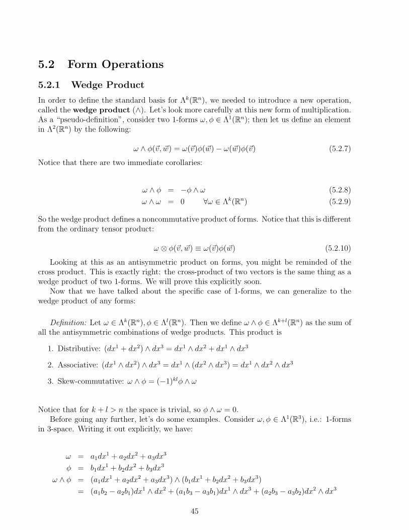
5.2 Form Operations

5.2.1 Wedge Product

In order to define the standard basis for Λk(Rn), we needed to introduce a new operation,called the wedge product (∧). Let’s look more carefully at this new form of multiplication.As a “pseudo-definition”, consider two 1-forms ω, φ ∈ Λ1(Rn); then let us define an elementin Λ2(Rn) by the following:

ω ∧ φ(~v, ~w) = ω(~v)φ(~w)− ω(~w)φ(~v) (5.2.7)

Notice that there are two immediate corollaries:

ω ∧ φ = −φ ∧ ω (5.2.8)

ω ∧ ω = 0 ∀ω ∈ Λk(Rn) (5.2.9)

So the wedge product defines a noncommutative product of forms. Notice that this is differentfrom the ordinary tensor product:

ω ⊗ φ(~v, ~w) ≡ ω(~v)φ(~w) (5.2.10)

Looking at this as an antisymmetric product on forms, you might be reminded of thecross product. This is exactly right: the cross-product of two vectors is the same thing as awedge product of two 1-forms. We will prove this explicitly soon.

Now that we have talked about the specific case of 1-forms, we can generalize to thewedge product of any forms:

Definition: Let ω ∈ Λk(Rn), φ ∈ Λl(Rn). Then we define ω ∧ φ ∈ Λk+l(Rn) as the sum ofall the antisymmetric combinations of wedge products. This product is

1. Distributive: (dx1 + dx2) ∧ dx3 = dx1 ∧ dx2 + dx1 ∧ dx3

2. Associative: (dx1 ∧ dx2) ∧ dx3 = dx1 ∧ (dx2 ∧ dx3) = dx1 ∧ dx2 ∧ dx3

3. Skew-commutative: ω ∧ φ = (−1)klφ ∧ ω

Notice that for k + l > n the space is trivial, so φ ∧ ω = 0.Before going any further, let’s do some examples. Consider ω, φ ∈ Λ1(R3), i.e.: 1-forms

in 3-space. Writing it out explicitly, we have:

ω = a1dx1 + a2dx

2 + a3dx3

φ = b1dx1 + b2dx

2 + b3dx3

ω ∧ φ = (a1dx1 + a2dx

2 + a3dx3) ∧ (b1dx

1 + b2dx2 + b3dx

3)

= (a1b2 − a2b1)dx1 ∧ dx2 + (a1b3 − a3b1)dx1 ∧ dx3 + (a2b3 − a3b2)dx2 ∧ dx3

45

Notice how I’ve been careful to keep track of minus signs. Also notice that this looksvery similar to a cross product, as stated earlier. What about taking the wedge product oftwo 1-forms in R4:

ξ = a1dx1 + a2dx

2 + a3dx3 + a4dx

4

χ = b1dx1 + b2dx

2 + b3dx3 + b4dx

4

ξ ∧ χ = (a1b2 − a2b1)dx1 ∧ dx2 + (a1b3 − a3b1)dx1 ∧ dx3 + (a1b4 − a4b1)dx1 ∧ dx4

+(a2b3 − a3b2)dx2 ∧ dx3 + (a2b4 − a4b2)dx2 ∧ dx4 + (a3b4 − a4b3)dx3 ∧ dx4

Note that this does not look like a “cross product”; it is a six-dimensional object in R4.However, if you took another wedge product with another 1-form, you would get a 3-form inR4 (which is four-dimensional), and that would give you something like a four-dimensionalcross product. In general, taking the wedge product of (n − 1) 1-forms in Rn will give yousomething analogous to a cross-product. We’ll get back to this later.

As a final example, what if you took the wedge product of a 1-form and a 2-form in R3:

α = c1dx1 + c2dx

2 + c3dx3 (5.2.11)

β = L12dx1 ∧ dx2 + L13dx

1 ∧ dx3 + L23dx2 ∧ dx3 (5.2.12)

α ∧ β = (c1L23 − c2L13 + c3L12)dx1 ∧ dx2 ∧ dx3 (5.2.13)

Notice that if we identify β = ω ∧ φ from above, then we have shown that the triple wedgeproduct of 1-forms in R3 is just:

ω ∧ φ ∧ α = det

a1 a2 a3

b1 b2 b3

c1 c2 c3

dx1 ∧ dx2 ∧ dx3 (5.2.14)

In fact, the wedge product of n 1-forms in Rn is always such a determinant. This is avery important fact that will come up again and again.

Next, we can ask how a general wedge product of forms acts on vectors? The answer isthat the form farthest to the left acts on the vector, and then you must permute the form sothat all the 1-forms act on the vector. As an example, consider a 2-form acting on a vector:

dx ∧ dy(~v) = dx(~v)dy − dy(~v)dx = vxdy − vydxThe minus sign comes from flipping the dx and the dy.

Before moving on, let us conclude this section with a definition and a theorem:

Definition: A simple k-form is a “monomial” k-form; that is, there is no addition.

Theorem: All k-forms can be written as a linear combination of simple k-forms.

Proof: The proof of this theorem is straightforward: a simple k-form is just a basiselement, possibly multiplied by a number. Then since we are dealing with a vector space,any element of Λk(Rn) can be written as a linear combination of these basis elements. QED.

46

5.2.2 Tilde

The tilde operator is the operator that translates us from vectors to forms, and vice versa.In general, it is an operation: (rank-k tensors) 7→(k-forms). Let’s see some examples:

~v = v1~e1 + v2~e2 + v3~e3 ∈ R3

v = v1dx1 + v2dx

2 + v3dx3 ∈ Λ1(R3)

Notice that the tilde changed subscript indices to superscript. This is important when wehave to keep track of what is covariant and contravariant.

Let’s do another less trivial example:

L =

0 L12 L13

−L12 0 L23

−L13 −L23 0

∈ R3 (Rank-2)

L =(L12dx

1 ∧ dx2 + L13dx1 ∧ dx3 + L23dx

2 ∧ dx3)∈ Λ2(R3)

=1

2Lijdx

i ∧ dxj

where in the last line I’m using Einstein notation for the indices. Notice how much simplerit is to write a 2-form as opposed to writing a rank-2 tensor. Also note that both Lij andLji are taken care of, including the minus sign, by using wedge products as opposed to usingtensor products - this is why we need the factor of 1

2in the last line. We are beginning to

see why form notation can be so useful!Incidentally, notice that I am only considering antisymmetric tensors when I talk about

forms. This is because the form notation has antisymmetry built into it. For symmetrictensors, the concept of a form is not very useful.

Finally, let me state a pretty obvious result:

Theorem: ˜v = v.

Proof: Left to the reader.

5.2.3 Hodge Star

The next tool we introduce for differential forms is the Hodge Star (∗). The Hodge Starconverts forms to their so-called dual form:

∗ : Λk(Rn)→ Λn−k(Rn) (5.2.15)

As for many other things in linear algebra, it is sufficient to consider how the Hodge staracts on the basis elements. Let’s look at some examples.

In R2:

∗dx1 = dx2

∗dx2 = −dx1

47

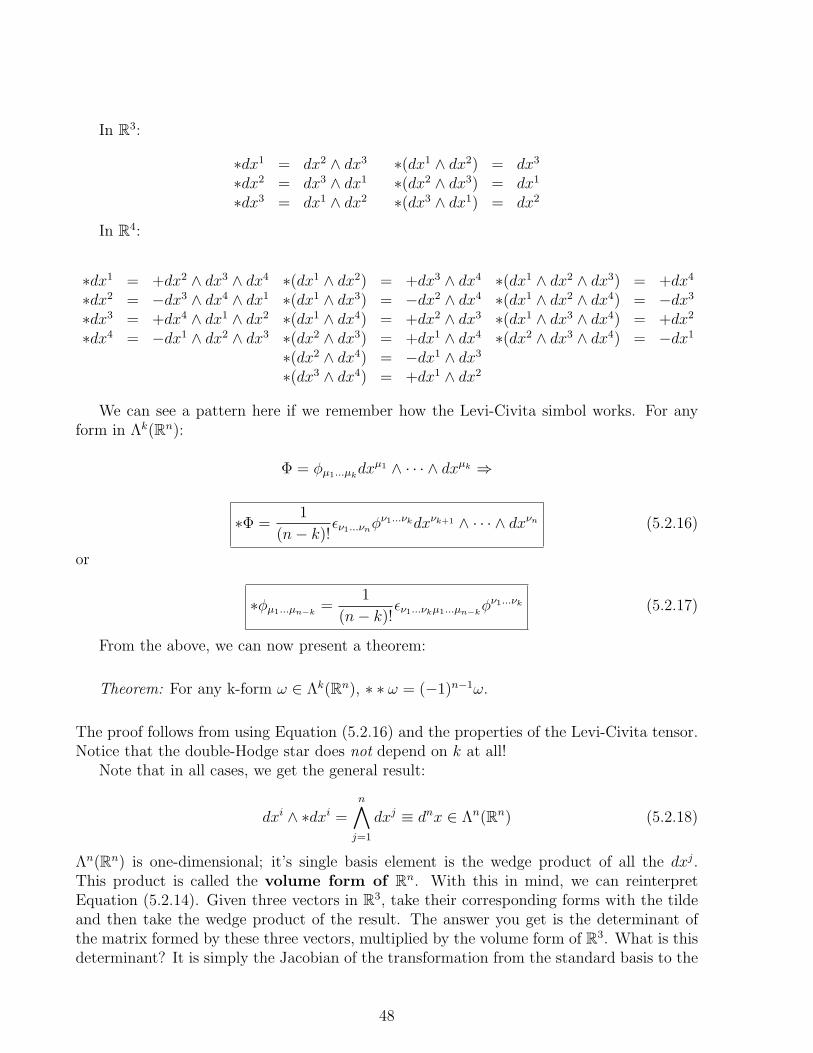
In R3:

∗dx1 = dx2 ∧ dx3 ∗(dx1 ∧ dx2) = dx3

∗dx2 = dx3 ∧ dx1 ∗(dx2 ∧ dx3) = dx1

∗dx3 = dx1 ∧ dx2 ∗(dx3 ∧ dx1) = dx2

In R4:

∗dx1 = +dx2 ∧ dx3 ∧ dx4 ∗(dx1 ∧ dx2) = +dx3 ∧ dx4 ∗(dx1 ∧ dx2 ∧ dx3) = +dx4

∗dx2 = −dx3 ∧ dx4 ∧ dx1 ∗(dx1 ∧ dx3) = −dx2 ∧ dx4 ∗(dx1 ∧ dx2 ∧ dx4) = −dx3

∗dx3 = +dx4 ∧ dx1 ∧ dx2 ∗(dx1 ∧ dx4) = +dx2 ∧ dx3 ∗(dx1 ∧ dx3 ∧ dx4) = +dx2

∗dx4 = −dx1 ∧ dx2 ∧ dx3 ∗(dx2 ∧ dx3) = +dx1 ∧ dx4 ∗(dx2 ∧ dx3 ∧ dx4) = −dx1

∗(dx2 ∧ dx4) = −dx1 ∧ dx3

∗(dx3 ∧ dx4) = +dx1 ∧ dx2

We can see a pattern here if we remember how the Levi-Civita simbol works. For anyform in Λk(Rn):

Φ = φµ1...µkdxµ1 ∧ · · · ∧ dxµk ⇒

∗Φ =1

(n− k)!εν1...νnφ

ν1...νkdxνk+1 ∧ · · · ∧ dxνn (5.2.16)

or

∗φµ1...µn−k =1

(n− k)!εν1...νkµ1...µn−kφ

ν1...νk (5.2.17)

From the above, we can now present a theorem:

Theorem: For any k-form ω ∈ Λk(Rn), ∗ ∗ ω = (−1)n−1ω.

The proof follows from using Equation (5.2.16) and the properties of the Levi-Civita tensor.Notice that the double-Hodge star does not depend on k at all!

Note that in all cases, we get the general result:

dxi ∧ ∗dxi =n∧j=1

dxj ≡ dnx ∈ Λn(Rn) (5.2.18)

Λn(Rn) is one-dimensional; it’s single basis element is the wedge product of all the dxj.This product is called the volume form of Rn. With this in mind, we can reinterpretEquation (5.2.14). Given three vectors in R3, take their corresponding forms with the tildeand then take the wedge product of the result. The answer you get is the determinant ofthe matrix formed by these three vectors, multiplied by the volume form of R3. What is thisdeterminant? It is simply the Jacobian of the transformation from the standard basis to the

48

basis of the three vectors you chose! In other words, differential forms automatically give usthe vector calculus result:

dn~x′ = J dn~x (5.2.19)

5.2.4 Evaluating k-Forms

We have done a lot of defining, but not too much calculating. You might be asking at thispoint: OK, so we have all of this machinery- now what?

The appearance of determinants should give you a clue. Whenever we need to evaluatea k-form, we construct a matrix according to the prescription the form gives us. Finally, wetake the determinant of the matrix.

To construct the matrix, we simply chose whatever elements of our vectors get pickedout by the simple form.

Examples: evalutate the following forms:

1.

dx ∧ dy

abc

,

def

2.

dx ∧ dz

abc

,

def

3.

dx ∧ dy ∧ dz

abc

,

def

,

ghi

Answers:

1. Construct the matrix by picking out the “x” and “y” components of the vectors, andtake the determinant:

det

(a db e

)2. This is similar, but now pick out the “x” and “z” components:

det

(a dc f

)3. For this case, it is simply what we had before:

det

a d gb e hc f i

Hopefully you get the hang of it by now.

49

5.2.5 Generalized Cross Product

Eariler, I mentioned that we can define a generalized cross product in Rn by wedging together(n− 1) 1-forms. Let’s see this explicitly:

In Rn, take n− 1 vectors, and tilde them so they are now 1-forms: v1, . . . , vn−1. Nowwedge these forms together to give you an (n − 1)-form, and take the Hodge star of theproduct to give us a 1-form. Finally tilde the whole thing to give us an n-vector, and wehave defined a general product of vectors:

~v1 × · · · × ~vn−1 ≡ ˜[∗(v1 ∧ · · · ∧ vn−1)] ∈ Rn (5.2.20)

5.3 Exterior Calculus

A k-form field is a k-form whose coefficients depend on the coordinates. This is exactlyanalogous to a vector field in vector calculus. So, if we have a vector field in R3:

~v(~x) = v1(~x)~e1 + v2(~x)~e2 + v3(~x)~e3

v(~x) = v1(~x)dx1 + v2(~x)dx2 + v3(~x)dx3

5.3.1 Exterior Derivative

Now that we have a notion of “function”, let’s see what we can do in the way of calculus.We can define an operator

d : Λk(Rn)→ Λk+1(Rn)

with the all-important property:

d2 = dd ≡ 0 (5.3.21)

By construction we will let d act on forms in the following way:

d(a(x)dx) = da(x) ∧ dx (5.3.22)

Let’s look at some examples.

f(~x) ∈ Λ0(R3)→ df(~x) =

(∂f

∂x1

)dx1 +

(∂f

∂x2

)dx2 +

(∂f

∂x3

)dx3 ∈ Λ1(R3)

This is just the gradient of a function! How about the curl?

50

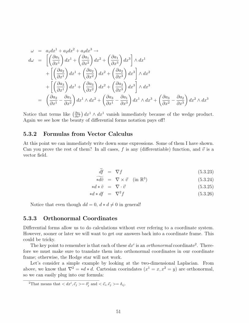
ω = a1dx1 + a2dx

2 + a3dx3 →

dω =

[(∂a1

∂x1

)dx1 +

(∂a1

∂x2

)dx2 +

(∂a1

∂x3

)dx3

]∧ dx1

+

[(∂a2

∂x1

)dx1 +

(∂a2

∂x2

)dx2 +

(∂a2

∂x3

)dx3

]∧ dx2

+

[(∂a3

∂x1

)dx1 +

(∂a3

∂x2

)dx2 +

(∂a3

∂x3

)dx3

]∧ dx3

=

(∂a2

∂x1− ∂a1

∂x2

)dx1 ∧ dx2 +

(∂a3

∂x1− ∂a1

∂x3

)dx1 ∧ dx3 +

(∂a3

∂x2− ∂a2

∂x3

)dx2 ∧ dx3

Notice that terms like(∂a1

∂x1

)dx1 ∧ dx1 vanish immediately because of the wedge product.

Again we see how the beauty of differential forms notation pays off!

5.3.2 Formulas from Vector Calculus

At this point we can immediately write down some expressions. Some of them I have shown.Can you prove the rest of them? In all cases, f is any (differentiable) function, and ~v is avector field.

df = ∇f (5.3.23)

∗dv = ∇× ~v (in R3) (5.3.24)

∗d ∗ v = ∇ · ~v (5.3.25)

∗d ∗ df = ∇2f (5.3.26)

Notice that even though dd = 0, d ∗ d 6= 0 in general!

5.3.3 Orthonormal Coordinates

Differential forms allow us to do calculations without ever refering to a coordinate system.However, sooner or later we will want to get our answers back into a coordinate frame. Thiscould be tricky.

The key point to remember is that each of these dxi is an orthonormal coordinate2. There-fore we must make sure to translate them into orthonormal coordinates in our coordinateframe; otherwise, the Hodge star will not work.

Let’s consider a simple example by looking at the two-dimensional Laplacian. Fromabove, we know that ∇2 = ∗d ∗ d. Cartesian coorindates (x1 = x, x2 = y) are orthonormal,so we can easily plug into our formula:

2That means that < dxi, ~ej >= δij and < ~ei, ~ej >= δij .

51

df =∂f

∂xdx+

∂f

∂ydy

∗df =∂f

∂xdy − ∂f

∂ydx

d ∗ df =∂2f

∂x2dx ∧ dy − ∂2f

∂y2dy ∧ dx

=

[∂2f

∂x2+∂2f

∂y2

]dx ∧ dy

∗d ∗ df =∂2f

∂x2+∂2f

∂y2

All is well with the world. But what if I wanted to do my work in polar coordinates?Then my coordinate system is (x1 = r, x2 = θ), but the orthonormal polar coordinate basis

vectors are ~e1 = r,~e2 = θr, and the dual basis is (dr, rdθ) (see previous footnote). So:

df =∂f

∂rdr +

∂f

∂θdθ(rr

)=∂f

∂rdr +

1

r

∂f

∂θ(rdθ)

∗df =∂f

∂r(rdθ)− 1

r

∂f

∂θdr

d ∗ df =

∂

∂r

(r∂f

∂r

)dr ∧ dθ − ∂

∂θ

(1

r

∂f

∂θ

)dθ ∧ dr

(rr

)=

[1

r

∂

∂r

(r∂f

∂r

)+

1

r2

∂2f

∂θ2

]dr ∧ (rdθ)

∗d ∗ df =1

r

∂

∂r

(r∂f

∂r

)+

1

r2

∂2f

∂θ2= ∇2f Wow!

where I have introduced ( rr) in the first and third line in order to keep the coordinates

orthonormal before using the Hodge star. So, as long as we are careful to use orthonormalcoordinates when using the Hodge star, our formulas work for any coordinate system! Thisis a vital reason why differential forms are so useful when working with general relativity,where you want to prove things about the physics independent of your reference frame orcoordinate basis.

5.4 Integration

We have discussed how to differentiate k-forms; how about integrating them? First I willdiscuss how to formally evaluate forms, and then I will present a formula for integratingthem. With this definition in mind, we will be able to derive Stokes’ Theorem- possibly themost important theorem differential forms will provide us with.

52

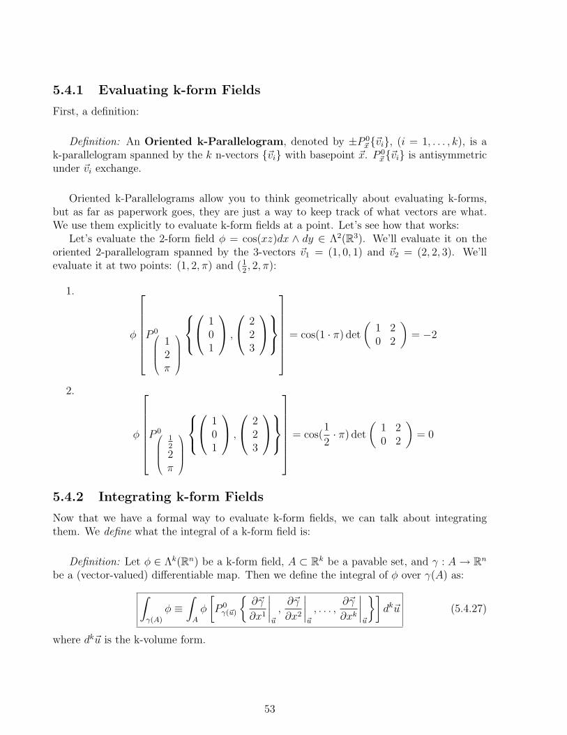
5.4.1 Evaluating k-form Fields

First, a definition:

Definition: An Oriented k-Parallelogram, denoted by ±P 0~x~vi, (i = 1, . . . , k), is a

k-parallelogram spanned by the k n-vectors ~vi with basepoint ~x. P 0~x~vi is antisymmetric

under ~vi exchange.

Oriented k-Parallelograms allow you to think geometrically about evaluating k-forms,but as far as paperwork goes, they are just a way to keep track of what vectors are what.We use them explicitly to evaluate k-form fields at a point. Let’s see how that works:

Let’s evaluate the 2-form field φ = cos(xz)dx ∧ dy ∈ Λ2(R3). We’ll evaluate it on theoriented 2-parallelogram spanned by the 3-vectors ~v1 = (1, 0, 1) and ~v2 = (2, 2, 3). We’llevaluate it at two points: (1, 2, π) and (1

2, 2, π):

1.

φ

P00BBB@

12π

1CCCA

1

01

,

223

= cos(1 · π) det

(1 20 2

)= −2

2.

φ

P00BBB@

12

2π

1CCCA

1

01

,

223

= cos(

1

2· π) det

(1 20 2

)= 0

5.4.2 Integrating k-form Fields

Now that we have a formal way to evaluate k-form fields, we can talk about integratingthem. We define what the integral of a k-form field is:

Definition: Let φ ∈ Λk(Rn) be a k-form field, A ⊂ Rk be a pavable set, and γ : A→ Rn

be a (vector-valued) differentiable map. Then we define the integral of φ over γ(A) as:∫γ(A)

φ ≡∫A

φ

[P 0γ(~u)

∂~γ

∂x1

∣∣∣∣~u

,∂~γ

∂x2

∣∣∣∣~u

, . . . ,∂~γ

∂xk

∣∣∣∣~u

]dk~u (5.4.27)

where dk~u is the k-volume form.

53

Like in vector calculus, we can define the integral formally in terms of Riemann sums -yuck! Let me just say that this is an equivalent definition; the more curious students can goprove it.

Let’s do two examples to get the hang of it:

1. Consider φ ∈ Λ1(R2) and integrate over the map:

γ(u) =

(R cosuR sinu

)over the region A = [0, α], (α > 0). Let φ = xdy − ydx:

∫γ(A)

φ =

∫[0,α]

(xdy − ydx)

P 00@ R cosuR sinu

1A(−R sinuR cosu

) du=

∫ α

0

du[(R cosu)(R cosu)− (R sinu)(−R sinu)]

=

∫ α

0

duR2[cos2 u+ sin2 u]

= αR2

2. Consider φ = dx ∧ dy + ydx ∧ dz ∈ Λ2(R3), and the map:

γ

(st

)=

s+ ts2

t2

over the region C =

(st

)|0 ≤ s ≤ 1, 0 ≤ t ≤ 1:

∫γ(C)

φ =

∫ 1

0

∫ 1

0

(dx ∧ dy + ydx ∧ dz)

P00BBB@s+ ts2

t2

1CCCA

1

2s0

,

102t

dsdt

=

∫ 1

0

∫ 1

0

[det

(1 12s 0

)+ s2 det

(1 10 2t

)]dsdt

=

∫ 1

0

∫ 1

0

(−2s+ 2s2t)dsdt

=

∫ 1

0

ds(−2s+ s2) = −2

3

54

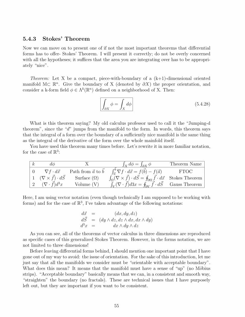
5.4.3 Stokes’ Theorem

Now we can move on to present one of if not the most important theorems that differentialforms has to offer- Stokes’ Theorem. I will present it correctly; do not be overly concernedwith all the hypotheses; it suffices that the area you are integrating over has to be appropri-ately “nice”.

Theorem: Let X be a compact, piece-with-boundary of a (k+1)-dimensional orientedmanifold M⊂ Rn. Give the boundary of X (denoted by ∂X) the proper orientation, andconsider a k-form field φ ∈ Λk(Rn) defined on a neighborhood of X. Then:∫

∂X

φ =

∫X

dφ (5.4.28)

What is this theorem saying? My old calculus professor used to call it the “Jumping-dtheorem”, since the “d” jumps from the manifold to the form. In words, this theorem saysthat the integral of a form over the boundary of a sufficiently nice manifold is the same thingas the integral of the derivative of the form over the whole mainfold itself.

You have used this theorem many times before. Let’s rewrite it in more familiar notation,for the case of R3:

k dφ X∫Xdφ =

∫∂Xφ Theorem Name

0 ∇f · d~x Path from ~a to ~b∫ ~b~a∇f · d~x = f(~b)− f(~a) FTOC

1 (∇× ~f) · d~S Surface (Ω)∫

Ω(∇× ~f) · d~S =

∮∂Ω~f · d~x Stokes Theorem

2 (∇ · ~f)d3x Volume (V)∫V

(∇ · ~f)d3x =∮∂V

~f · d~S Gauss Theorem

Here, I am using vector notation (even though technically I am supposed to be working withforms) and for the case of R3, I’ve taken advantage of the following notations:

d~x = (dx, dy, dz)

d~S = (dy ∧ dz, dz ∧ dx, dx ∧ dy)d3x = dx ∧ dy ∧ dz

As you can see, all of the theorems of vector calculus in three dimensions are reproducedas specific cases of this generalized Stokes Theorem. However, in the forms notation, we arenot limited to three dimensions!

Before leaving differential forms behind, I should mention one important point that I havegone out of my way to avoid: the issue of orientation. For the sake of this introduction, let mejust say that all the manifolds we consider must be “orientable with acceptable boundary”.What does this mean? It means that the manifold must have a sense of “up” (no Mobiusstrips). “Acceptable boundary” basically means that we can, in a consistent and smooth way,“straighten” the boundary (no fractals). These are technical issues that I have purposelyleft out, but they are important if you want to be consistent.

55

5.5 Forms and Electrodynamics

As a finale for differential forms, I thought it would be nice to summarize briefly how oneuses forms in theories such as E&M. Recall that in covariant electrodynamics, we have anantisymmetric, rank-2 4-tensor known as the “Field Strength” tensor:

F ≡ Fµνdxµ ⊗ dxν (5.5.29)

As we have seen, it is always possible to use 2-forms instead of (antisymmetric) tensors, andwe can rewrite the above tensor as a differential form in Λ2(M4)3:

F ≡ 1

2Fµνdx

µ ∧ dxν ∈ Λ2(M4) (5.5.30)

Notice that the antisymmetry of Fµν is immediate in form notation. Also, this is a 2-form infour dimensions, which means that its dual is also a 2-form. Now using Equation (5.5.30), Ican write the Lorentz Force Law for a particle with charge e moving with a velocity vector~u as:

˙p = eF (~u) ∈ Λ1(M4) (5.5.31)

Let’s consider an example. Suppose we have a magnetic field in the x direction, soF = Bxdy ∧ dz. Then the force on the particle is:

˙p = eF (~u) = eBx 〈dy ∧ dz, ~u〉= eBx[dy 〈dz, ~u〉 − dz 〈dy, ~u〉]= eBx[uzdy − uydz]⇒ ~p = eBx(uzy − uyz)

This is exactly what you would have gotten if you had used your vector-form of Lorentz’sLaw, with cross products.

Another vector that is important in E&M is the 4-current (J). We will again think of Jas a 1-form in M4; therefore, it’s dual is a 3-form.

Armed with all we need, we can write down Maxwell’s Equations:

dF = 0 (5.5.32)

d ∗ F = 4π ∗ J (5.5.33)

To interpret these equations, one can think of F (∗F ) as an object that represents “tubes offorce” flowing through space-time.

We can take advantage of Stokes Theorem (just like in regular vector calculus) to putthese equations in integral form:

3M4 is Minkowski space-time. In general, I can go to any space I want; for now, I’m sticking to flat space(i.e.: ignoring gravity). But notice that this analysis is totally general, and gravity can be easily included atthis stage.

56

∫Σ

dF =

∮∂Σ

F = 0 (5.5.34)∫Σ

d ∗ F =

∮∂Σ

∗F = 4π(charge) (5.5.35)

The first of these equations says that the total flux of F through a closed region of space-time is zero; the second equation says that the total flux of ∗F through a closed region ofspace-time is proportional to the amount of charge in that region. Notice that this descriptionnever mentions coordinate systems: once again, differential forms has allowed us to describephysics and geometry without ever referring to a coordinate system! Notice the similarityof this equation with the Gauss-Bonnet Theorem – in gauge theories, you may think of thefield strength as a curvature to some space!

The final step in studying electrodynamics is to notice that Equation (5.5.32) suggestssomething. Recall that if a differential form was the exterior derivative of some other form,then it’s exterior derivative was necessarely zero, via Equation (5.3.21). Is the converse true?Namely, if you have a form whose exterior derivative is zero, can it be written as the exteriorderivative of some other form?

Your first impulse might be to say “yes”: surely if the form is an exterior derivative, yourcondition is satisfied. But it turns out that the question is a little more subtle than that.For I can give you a form which is not an exterior derivative of another form, and yet stillhas vanishing exterior derivative! This is a famous case of “necessity” versus “sufficiency”in mathematics. That a form is an exterior derivative is sufficient for its exterior derivativeto vanish, but not necessary.

The key point is that this property depends not on the differential forms themselves, buton the global properties of the space they live in! It turns out that M4 does indeed have theproperty of necessity; specifically, it is simply connected. Therefore it is safe to assume a laEquation (5.5.32) that we can write:

F = dA (5.5.36)

for some 1-form A. So indeed, electrodynamics in flat space can be described by a 4-vectorpotential. But do be careful not to jump to any conclusions before you know the propertiesof the universe you are describing!

Finally, we can consider what happens if we let A→ A+ dλ, where λ is any (reasonablywell-behaved) function. Then by just plugging into Equation (5.5.36), with the help ofEquation (5.3.21), we see that F remains the same. Hense, the 4-vector potential is onlydefined up to a 4-gradient; this is exactly what gauge invariance tells us should happen!

This gives a very powerful geometric intuition for our field-strength, and therefore forelectricity and magnetism. You can do similar analyses for any gauge field, and by adjustingthe manifold, you can alter your theory to include gravity, extra dimensions, strings, orwhatever you want! This is one of the biggest reasons why differential forms are so useful tophysicists.

57

Chapter 6

Complex Analysis

In this chapter, I would like to present some key results that are used in analytic work. Thereis of course much more material that what I present here, but hopefully this small reviewwill be useful.

Complex analysis is concerned with the behavior of functions of complex variables. Itturns out that these functions have a much different behavior than functions of real variables.The techniques of complex analysis, pioneered in the eighteenth and nineteenth centuries,have become very important in almost all branches of applied mathematics. I am assum-ing that you are familiar with the basics of complex numbers (z = x + iy ∈ C) and willimmediately move on.

In my experience, applications of complex numbers fall into two general catagories:Cauchy’s Integral Theorem and Conformal Mapping. This review will consider the cal-culus of complex variables. I will not mention too much about conformal mapping, exceptto define it and give an example or two.

Complex numbers are written as z. Then a function of a complex variable has the form:

f(z) = f(x+ iy) = u(x, y) + iv(x, y)

where u, v are both real valued functions of the real variables x, y. You can also write acomplex number in polar coordinates z = reiθ, where r ≡ |z| and θ is called the argmentof z, sometimes denoted as arg z.

6.1 Analytic Functions

• Definition: A complex function f(z) is analytic at a point z0 if it has a Taylorexpansion that converges in a neighborhood of that point:

f(z) =∞∑i=0

ai(z − z0)i

If f(z) is analytic at all points inside some domain D ⊂ C then it is said to be analyticin D. If it is analytic for all finite complex numbers, it is said to be entire. If it isanalytic for all complex numbers, including infinity, then f(z) =constant!

58

• Theorem: The real and imaginary parts of an analytic function f(z) = u(x, y)+iv(x, y)satisfy the Cauchy-Riemann (CR) Equations:

ux = vy (6.1.1)

vx = −uy (6.1.2)

where ux means the partial derivative of u with respect to x, etc. From the CRequations, it can be seen that both u and v satisfy Laplace’s equation:

uxx + uyy = vxx + vyy = 0

Functions that satisfy Laplace’s equation are called harmonic functions. If u(x, y) isa harmonic function, then up to an additive constant, there is a unique function v(x, y)that satisfies the CR equations with u(x, y). This function is called the harmonicconjugate of u(x, y). Notice that this relation is not reflexive in general; in otherwords, if v is the harmonic conjugate of u, then it is not generally true that u is theharmonic conjugate of v. When it is true, it is possible to show that u and v areconstants.

• Let’s do an example:f(z) = z2 = (x2 − y2) + i(2xy)

This function is analytic everywhere in the finite complex plane (it is entire): its Taylorseries about z = 0 is trivial: a2 = 1, all others zero. It also satisfies the CR equations.Note that the function v(x, y) = 2xy is the harmonic conjugate to u(x, y) = x2 − y2,but as we expect from the above note, the converse is not true (prove it!).

• Let’s see how one might construct the harmonic conjugate of a real-valued harmonicfunction. Consider the function u(x, y) = y3−3x2y. This function is certainly harmonic(prove it!), so up to an additive constant, there should be a unique function v(x, y)that is the harmonic conjugate of u(x, y). To find it, note first of all that by the firstCR equation, vy = ux = −6xy. Integrating this equation with respect to y givesv(x, y) = −3xy2 +φ(x) where φ(x) is some arbitrary function of x alone. Plugging intothe second CR equation gives φ′(x) = 3x2. Integrating this gives φ(x) = x3 +C with anarbitrary constant C, and therefore v(x, y) = x3− 3xy2 +C is the harmonic conjugateto u(x, y). Therefore f(x, y) = u(x, y)+iv(x, y) must be an analytic function. Exercise:show that f(x, y) can be rewritten as f(z) = i(z3 + C), which is certainly analytic.

• Consider two analytic functions f1(z), f2(z) defined on domains D1, D2 respectively,where D1 ∩ D2 6= ∅. Also assume that the two functions agree for all points in theintersection. Then f2(z) is called the analytic continuation of f1(z). When ananalytic continuation exists, then it is unique. The proof of this is not hard, but thekey is in the analytic. This means that there is only one way to “extend” a functionanalytically out of its original domain. Notice, however, that if f3(z) is another analyticcontinuation of f2(z) into another domain D3, it need not be a continuation of f1(z)into that domain!

59

• As an example, let’s look at our old example of f(z) = z2. This function agrees withthe function f(x) = x2 in the domain of real numbers (y = 0). It is also analytic,therefore it is the analytic continuation of the real-valued function f(x) = x2. Further,it is unique: there is no other function that is analytic and matches with our originalfunction!

• That was an obvious one. What about a more complicated example? Consider thefactorial function defined on N: f(n) = n! I will now define a function on the realnumbers:

Γ(x) =

∫ ∞0

dssx−1e−s (6.1.3)

Integrating by parts shows that when x is a natural number, Γ(x) = (x− 1)! Further-more, Γ(x) is in fact an analytic function of x, so long as x is not a negative integeror zero. Hense, Γ(x) is the (unique) analytic continuation of the factorial function tothe real numbers (without the negative integers or zero). Indeed, we can go further:by replacing x → z (as long as z is not a negative integer or zero – why not?) thisextends to all of C.

6.2 Singularities and Residues

• Definition: A Laurent Expansion of a function f(z) about a point z0 is an expansionin both positive and negative powers:

f(z) =∞∑

n=−∞

cn(z − z0)n =∞∑n=1

b−n(z − z0)n

+∞∑n=0

an(z − z0)n (6.2.4)

• As you can see, a Laurent expansion is a generalization of a Taylor expansion. Noticethat the function is not defined at the point z0 unless all of the bn = 0. If this is thecase, f(z) is analytic at z0. A Taylor expansion typically exists in an open disk aboutthe point z0. The generalization to the Laurent expansion converges inside an annulusR1 < |z − z0| < R2.

• A singularity of a function is a point where the function is not defined. If z0 is asingularity of f(z) and you can define a neighborhood (open set) about that point U(z0)such that f(z) is analytic in the domain U(z0) − z0 (so R1 → 0 above), then z0 iscalled an isolated singularity. There are three general types of isolated singularities:

1. Removable singularities are the most mild form of singularity, where all theb−n = 0. An example of this is the function sinx

x. This function is not defined

at the origin, but it does have a well-defined limit there. You can see this byperforming a Taylor expansion of the sine function and dividing out by x, leavinga finite value plus terms that are O(x) and hense vanish in the limit. Removablesingularities are trivial, and I will not talk anymore about them.

60

2. If a function has a Laurent expansion about z0 but there exists an integer m > 0such that all the b−n = 0 for every n > m (but with b−m 6= 0), then the function issaid to have a Pole of order m at z0. In the special case of m = 1, the functionis said to have a simple pole. An example of a function with a simple pole iscosxx

at the origin, where it behaves as 1/x. Poles are very useful and importantin complex analysis, as we will see.

3. If a function has a Laurent expansion about z0 but there is not an integer m > 0such that all the b−n = 0 for every n > m (so the denominator terms do not stop),then the function is said to have an Essential Singularity at z0. An example ofthis is the function f(z) = e1/z at the origin. This singularity is a true nightmare,and there is very little to be done for it!

• If a function f(z) has a pole of order m at z0 (not necessarely a simple pole), then thequantity b−1 is called the Residue of the pole, also denoted by Resz=z0

f(z)

. This

quantity plays a vital role in the calculus of complex-valued functions. A function thatis analytic in a domain, up to maybe a countable number of poles (so it still has aLaurent expansion), is said to be meromorphic in that domain.

• Residues are so important, I want to list various methods of finding them. I will stateseveral methods here without proof:

1. If p(z0) 6= 0 and q(z) has a zero of order m at z01 then p(z)

q(z)has a pole of order m

at z0.

2. If f(z) has a pole of order m at z0, it can be written as f(z) = p(z)(z−z0)m

where

p(z0) 6= 0. Then the residue of f(z) at z0 is b−1 = p(m−1)(z0)(m−1)!

3. If q(z) has a simple zero at z0 and p(z0) 6= 0, then the residue of p(z)q(z)

at z0 is given

by b−1 = p(z0)

q′ (z0)

• Before leaving this section, there is one more type of singularity that comes up. This isnot an isolated singularity, and therefore is not defined through its Laurant expansion.Rather this singularity comes from an ambiguity in multiply defined functions. Forexample, consider the complex Logarithmic function:

log z = log r + iθ

where I have used the famous result z = reiθ. The imaginary part of this functionis a problem, since θ is only defined up to an arbitrary factor of 2π. Therefore, thisexpression has an infinite number of solutions for a single value of z. In real analysis,we would throw such functions away, but not in complex analysis. The solution is todefine a cut where we explicitly say what values of θ we allow. For example, we cansay that we will only let −π < θ < +π. This is called the principle branch of thelogarithmic function, and is sometimes denoted Log z.

1i.e.: q(z) = (z − z0)mr(z), where r(z0) 6= 0.

61

• Branch cuts are lines in the complex plane that tell you where to cut off the definitionof your function. For example, the branch cut for the logarithmic function is a line thatconnects the origin to infinity. For the principle branch, that line extends along thenegative real axis. It could have gone in any direction, which would have correspondedto a different branch of the logarithm. In addition, it does not even have to be astraight line. Notice that the function is discontinuous as you cross the branch cut. Inthe case of the Logarithm: log(−x + iε) − log(−x − iε) = 2πi, where x is a positivereal number. Branch cuts are discontinuities in the function.

• The branch cut you make is not unique, but what is true is that all branch cuts connecttwo points, and those two points are unique. In the case of the Logarithm, those pointswere the origin and infinity. Since those points are common to all branch cuts, youcannot ever define the logarithmic function there. Therefore they are singularities.They are called branch points.

• Aside from the logarithm, the most common function with branch point singularitiesis the function f(z) = xa where 0 < Re(a) < 1. This function is multiply defined sincef(z) = f(zei2πn/a), for integer n. It too has branch points at z = 0,∞.

6.3 Complex Calculus

When doing calculus on a function of complex variables, a whole new world of possibilitiesopens up! At first, you can think of the complex plane as a special representation of R2, andyou might think that the complex calculus is the same as real vector calculus. But this isnot true! There are a variety of theorems that make calculus (especially integral calculus)on the complex plane a rich and fascinating subject, both theoretically as well as practically.

Complex analysis is a deep subject, but since this is supposed to be a practical review forphysics grad students, I will skip over all the proofs and just present the most commonly-used results. I strongly encourage you to read up on the theory behind this stuff; it’s reallyan amazing subject in and of itself.

• A general function of a complex variable can be written as f(z, z∗). Such a function isanalytic if and only if

df

dz∗≡ 0 (6.3.5)

so that f = f(z). Such a function is sometimes called holomorphic, but this is justa synonym for analytic.

• Just like in vector calculus, you can define contour integrals in the complex plane. ifC is a contour described by a path in the complex plane z(t) where t ∈ [a, b] is a realparameter, we can define the contour integral of an analytic function in terms of aone-dimensional Riemann integral:

62

∫C

f(z)dz ≡∫ b

a

f(z(t))z′(t)dt (6.3.6)

• Cauchy-Goursat Theorem: Let C be a closed contour in the complex plane and f(z)an analytic function on the domain interior to and on C. Then:∮

C

f(z)dz ≡ 0 (6.3.7)

This is a generalization of the fundamental theorem of calculus. A powerful conse-quence of this theorem is that a contour integral is invariant to deformations of thecontour, as long as the deformation does not pass through a singularity of f(z).

• Cauchy’s Integral Formula: Let f(z) be analytic everywhere within and on a simple,closed, positively oriented contour2 C, and let z0 be any point on the interior to C.Then:

f(z0) =1

2πi

∮C

f(z)dz

z − z0

(6.3.8)

• Using the Cauchy integral formula and some complex analysis, we can actually derivea very powerful formula for the n-th derivative of an analytic function:

f (n)(z) =n!

2πi

∮C

f(z)dz

(z − z0)n+1(6.3.9)

From this, we come to a rather amazing result: if a function is analytic (which is thesame as saying df

dzexists), then all of its derivatives exist and are given by the above

integral! This is very different from real analysis, where a function that has a firstderivative need not have higher derivatives. For example, x3/2 has a first derivative atx = 0 but it does not have a second derivative there. This kind of thing can neverhappen in complex analysis. Exercise: why doesn’t z3/2 contradict this result?

• Notice immediately the marvelous corollary to the above formulas: for all n ∈ Z,∮C

dz

(z − z0)n= 2πiδn1 (6.3.10)

as long as C encloses z0. This follows for n > 1 since the derivative of a constant iszero, and it follows for n ≤ 0 since such terms are analytic inside and on the contourand hence the integral vanishes by the Cauchy-Goursat theorem. Finally, the resultfor n = 1 follows directly from the Cauchy integral formula, or by direct integration.

2A positively oriented contour means you travel around the contour in a counter-clockwise direction; anegatively oriented contour travels around the contour in a clockwise direction.

63

• Using this result, we come to a remarkable and vital theorem used throughout all areasof applied and abstract mathematics. Consider a general, meromorphic function on thecomplex plane. Such a function has a Laurent expansion. Now let’s do a closed contourintegral, where we make sure the contour does not pass through any singularities off(z). Some of the isolated singularities of f(z) are on the interior of C (call this setZ = z0, z1, . . . , zn) and some are on the exterior, where Z can be a finite or infiniteset. Then we have the amazing and most important result:

∮C

f(z)dz = 2πi∑zk∈Z

Resz=zkf(z)

(6.3.11)

This result is usually called the Residue Theorem. This is why it’s so important toknow how to compute residues of meromorphic functions.

• To see how vitally useful the residue theorem is, consider the following real integral:

I =

∫ +∞

−∞

cosxdx

(x2 + a2)3(6.3.12)

Try doing this integral directly! Before you shoot yourself, let’s see how to do it injust a few steps. First of all, we analytically continue the integrand to the complexplane by replacing x by z (check that this is, indeed, the analytic continuation of theintegrand). Now in order to make sense of the cosine of a complex variable, we usethe definition cos z ≡ (eiz + e−iz)/2. We split the integral into two terms I = I+ + I−,where

I± =1

2

∫ +R

−R

e±izdz

(z2 + a2)3

where we will take the limit R → ∞ in the end. Let’s just consider I+ for now. Wecan rewrite the denominator as (z + ia)3(z − ia)3, so by rule 2 in the residues section,the integrand has a third-order pole at both of these points and the residue at thesepoints are given by

1

2!

d2

dz2

eiz

(z ± ia)3

∣∣∣∣z=±ia

= ∓i e∓a

16a5(3 + a(a± 3))

So far, we cannot apply the residue theorem since the contour is not closed. However,notice that when we go into the complex plane, the exponential in the numerator picksup a factor of e−Im(z). So in particular, if we add to I+ a term that is the contourintegral over the semicircle of radius R going through the upper-half of the complexplane (Im(z) > 0), such a term will go like e−R and hence vanish as R → ∞. If weinclude this term, we don’t change the value of I+ but we do close the contour, andhence can apply the residue theorem. Since we only surround the pole at z = +ia weonly keep that residue, and we get:

64

limR→∞

I+ =πe−a

16a5(3 + a(a+ 3))

To compute I−, the story is very similar, but there are a few differences to take intoaccount. First of all, with the exponential being negative, this will change our formulafor the residue slightly. Also, we will need to close the integral in the lower halfof the complex plane rather than the upper half, in order to make sure the addedcontribution vanishes. Finally, since the new contour is oriented clockwise rather thancounterclockwise, there is an extra negative sign. Putting this all together gives usthat I− = I+ so the final integral is∫ +∞

−∞

cosxdx

(x2 + a2)3=πe−a

8a5(3 + a(a+ 3))

Try doing that integral without the help of the residue theorem – I wouldn’t even knowwhere to begin!!

• The residue theorem gives us a way to integrate (or differentiate) complicated mero-morphic functions which are analytic on the contour of integration. But what aboutfunctions that have singularities on the contour? Such integrals by themselves are notwell-defined, but we can still make sense of them by means of a regulator. The finalanswer we get will not be unique since it will depend on the regularization scheme used.But once we specify this scheme, we can proceed to make well-defined statements.

• It turns out that there is a particular regularization scheme that is a very naturalchoice, called the Principle Value. As an example, consider the integral∫ ∞

−∞xdx

This integral is indeterminant until we chose precisely how to take the limit to infinity.The Principle Value of this integral is defined as the symmetric limit:

P∫ ∞−∞

xdx = limR→∞

∫ R

−Rxdx = 0

Notice that this choice of regulator is by no means unique. For example, we could havedefined the integral as

limR→∞

∫ R+ bR

−R− aR

xdx = b− a

• There is nothing special about any of these choices. However, there is good reason touse the principle value. Let f(x) be an analytic real-valued function. Then we havethe following vital result:

65

limε→0

∫ ∞−∞

f(x)

x− x0 ± iε= P

∫ ∞−∞

f(x)

x− x0

∓ iπf(x0) (6.3.13)

where the principle value on the right hand side should be understood as

P∫ ∞−∞

f(x)

x− x0

≡ limR→∞

limρ→0

(∫ −ρ−R

f(x)

x− x0

+

∫ R

ρ

f(x)

x− x0

)(6.3.14)

This theorem goes by many names, but I like to call it the Principle Value Theorem,although you might find it under something else in your favorite textbook.

• I will not prove the Principle Value theorem (it’s not very difficult to prove – try ityourself), but I will use it in a simple example. Let’s calculate the integral∫ ∞

−∞

cosx

x+ iεdx

As ε → 0, this integral is ill-definined, due to its pole on the real axis. Nonetheless,the Principle Value Theorem gives us a way to solve the problem:∫ ∞

−∞

cosx

x+ iε= P

∫ ∞−∞

cosx

x− iπ cos(0)

If the universe is fair, the first integral on the right-hand side should vanish due tothe symmetry of the integrand, but that will only happen if the divergences are undercontrol. Notice that near the origin, where the integrand has a simple pole, the principlevalue tells us how to cancel the divergence there:

limR→∞

limρ→0

(∫ −ρ−R

dx

x+

∫ R

ρ

dx

x

)= lim

R→∞limρ→0

(−∫ R

ρ

du

u+

∫ R

ρ

dx

x

)= 0

where I set u = −x in the first integral. Thus the principle value has tamed thedivergence. So this integral does exist, and it equals −iπ.

• Notice in the above example, if we had changed the sign of ε (placing the pole abovethe real axis rather than below it) we would have found a different answer +iπ, eventhough we take the limit ε → 0, and you might have thought that we should get thesame answer in the end. This is not a coincidence! It is due to the fact that the integral(without the ε) is not well defined. So this begs the question: which sign should weuse? This is where mathematics ends and physics begins. You will find that the choiceof sign typically comes from boundary conditions, and is sensitive to the particularproblem at hand.

66

• As a final example of how complex calculus is so very useful, let’s consider how tointegrate a function with a branch-point singularity. This is a little different since abranch point is not an isolated singularity, so the residue theorem doesn’t help by itself.But we can still do pretty well.

When there is a branch-point singularity, you have to specify a branch cut that connectsthe singularities. So for example, let’s consider the following integral:∫ ∞

0

x−adx

x+ 1

where 0 < a < 1. This integrand is multiply defined, so we must choose a branch cutto define it. This is a line connecting the two branch points, in this case the origin andinfinity. This comes from the fact that we can write the numerator as e−a log x. Also,notice the simple pole at x = −1, so we shouldn’t choose our branch cut to overlapwith that pole. We will make our cut along the positive real axis. This integral is thesame as ∫

R+

z−adz

z + 1

where the integral is along the positive real axis in the complex plane.

We will extend this contour: first, the contour goes from ρ + iε (ρ < 1) to R + iε(R > 1) on the real axis (L+). Then the contour goes counterclockwise around a circleof radius R until we get back to just below the real axis R − iε (CR). Then we travelback down the real axis until we get to ρ − iε (L−). Finally, we go clockwise arounda circle of radius ρ until we get back to the starting point at ρ + iε. The ε is there toavoid the branch cut - we can let ε→ 0 as long as we keep in mind how to define theexponent (see below). With our choice of ρ and R this contour encircles the pole, sothe residue theorem applies. So we have:(∫

L+

+

∫CR

+

∫L−

+

∫Cρ

)z−adz

z + 1= 2πie−iaπ

The two circle contour integrals vanish. To see that, we need the fact that |z1 + z2| ≥||z1| − |z2||. Then for the small circle:∣∣∣∣∣

∫Cρ

z−adz

z + 1

∣∣∣∣∣ ≤ ρ−a(2πρ)

||z| − 1|=

2π

1− ρρ1−a ρ→0−→ 0

and a similar analysis can be done with the large circle. The interesting part comesfrom the remaining two integrals. The integral across L+ is above the branch cut, solog z = log r + i0 as ε → 0, while the integral along L− is below the branch cut, solog z = log r + i2π as ε→ 0. Plugging this in:

67

∫L+

z−adz

z + 1=

∫ R

ρ

r−adr

r + 1

∫L−

z−adz

z + 1=

∫ ρ

R

r−ae2iaπdr

r + 1

Putting all of this together and taking the limits ρ→ 0 and R→∞ gives∫ ∞0

r−adr

r + 1=

2πie−iaπ

1− e2iaπ=

π

sin aπ

6.4 Conformal Mapping

• Conformal mapping is one of those tools that, in my experience, takes a great deal oftime and practice to get comfortable with. It is one of those things in mathematicswhich is almost as much art as science. Whole textbooks have been written on thisrich and amazing subject; perhaps it is overly ambitious for me to try and write thissection. But I’ve always loved a challenge.

I cannot begin to write a complete review of this subject – it would take way too longand I am not an expert on the subject anyway. So in this section I only intend topresent some of the basic theorems and one or two examples. Maybe one day I’ll domore than that, but not today.

• Conformal mapping is a technique that is useful in solving partial differential equationsin two dimensions with certain boundary conditions. The applications to such problemsrange everywhere from fluid dynamics to electrodynamics to financial forecasting! Thebasic idea is to transform complicated boundary conditions into simpler ones, and thusmake solving the problem much easier.

• Simply put, a conformal transformation is a transformation that preserves angles.Technically, consider a contour in the complex plane parametrized by a function z(t),and a map f(z) that is analytic and has a nonvanishing first derivative; such mapsare called conformal maps. Let w(t) = f(z(t)) be the image of the contour underthe map f . We will call the complex w-plane Cw and the complex z-plane Cz, sof : Cz → Cw.

• So what does this have to do with angles? The tangent vector in Cw is given by

w′(t) = f ′(z(t))z′(t)

From this it follows that

argw′(t) = arg f ′(z) + arg z′(t) (6.4.15)

Now let’s imagine two curves described by z1(t) and z2(t) that intersect at a pointz1(t0) = z2(t0) = z0 ∈ Cz. Then from the above formula, we have the result:

68

argw′1(t)− argw′2(t) = arg z′1(t)− arg z′2(t) (6.4.16)

So indeed we find that conformal transformations do preserve angles between contours.

• Before going further, let me point out a very important fact without proof: let f(z) =u(x, y)+iv(x, y) be an analytic function, so that u(x, y) and v(x, y) are both harmonic,and v is the harmonic conjugate to u. Let Tu(x, y) = ∇u(x, y) be the tangent vectorof u at the point (x, y), and similarly for Tv(x, y), and let (x0, y0) be a point such thatu(x0, y0) = v(x0, y0). Then Tu(x0, y0) · Tv(x0, y0) = 0; that is, harmonic conjugateshave orthogonal tangent vectors at points of intersection. I leave the proof of this toyou (Hint: use the CR Equations). This will be very useful in what follows.

• Another important fact: the definition of a conformal transformation turns out toprovide a necessary and sufficient condition for an inverse function to exist, at leastlocally; this is a result of the infamous “Inverse Function Theorem”. Thus, if we find aconformal transformation that simplifies our boundary conditions in Cw, we can alwaysinvert the transformation to get the solution on Cz, which is, of course, what we reallywant.

• The differential equation we are interested in is Laplace’s equation. Remember thatthe real and imaginary parts of an analytic function are harmonic functions; that is,solutions to Laplace’s equation in two dimensions. We are interested in two types ofboundary conditions for a harmonic function h(x, y) on a boundary described by acurve C in the complex plane z = x+ iy:

1. Dirichlet Boundary Conditions: h|C = h0 for any constant h0.

2. Neumann Boundary Conditions: ~n · ∇h|C = 0, where ~n is a unit vector normalto the boundary.

It turns out that for these two types of boundary conditions are preserved under con-formal transformations. Any other type of boundary condition will generally not bepreserved. for example, dh

dn

∣∣C

=constant6= 0 is not preserved by conformal transforma-tions. Therefore, whenever faced with trying to solve Laplace’s equation with eitherDirichlet or Neumann boundary conditions in two dimensions, conformal mapping isan available method of finding the solution. As mentioned above, this problem comesup many times and in many places, so this is a very powerful technique.

• As an example, let’s consider the problem of trying to find the electrostatic scalarpotential inside an electrical wire. The wire has a circular cross section, where half ofthe cylinder is kept at V = 0 and the other half is kept at V = 1. The cylindricalsymmetry of the problem means the potential cannot depend on z, so this is a two-dimensional problem. If we place the cross section of the wire on a unit circle in thecomplex plane Cz, we can look for a harmonic function that agrees with the boundaryconditions. This, by uniqueness of solutions, is the final answer. This is a Dirichletboundary condition problem with circular boundary. Such boundaries are complicated,but we can use conformal mapping to turn this problem into an easier one.

69

Consider the mapping:

w = i1− z1 + z

(6.4.17)

This is an example of a Mobius Transformation, also known as a linear fractionaltransformation . It has the effect of mapping the interior of the unit circle in Cz tothe entire upper-half plane of Cw, where the upper half of the circle is mapped to thepositive real w axis while the lower half of the circle is mapped to the negative real waxis. I leave it to you to prove that this map is, indeed, a conformal map.

Now the next step is to find a map on Cw that is harmonic and satisfies the boundaryconditions. Consider the function

1

πlogw =

1

π(log |w|+ i arg(w)) (6.4.18)

which is analytic and spans the upper half plane of Cw for 0 ≤ argw ≤ π. Notice thatthe imaginary part of this function satisfies the boundary conditions we need. Sinceit is the imaginary component of an analytic function is harmonic, so we found oursolution.

By writing w = u + iv, we have arg(w) = tan−1(vu

). By expanding Equation (6.4.17)

to compute u(x, y) and v(x, y), we find

V (~r) =1

πtan−1

(1− x2 − y2

2y

)=

1

πtan−1

(1− r2

2r sin θ

)(6.4.19)

where we take the branch of the arctangent function 0 ≤ tan−1 t ≤ π. It gets better:the harmonic conjugate of the potential is another harmonic function whose tangentvector is always orthogonal to the potential’s tangent vector. But the tangent vectorto the electrostatic potential is the electric field. And the lines perpendicular to thefield are just the field flux lines. From Equation (6.4.18) we know right away that theseflux lines are then given by the level curves of the imaginary part of −(i/π) logw, orupon using Equation (6.4.17):

E(~r) =1

2πlog

((1− x)2 + y2

(1 + x)2 + y2

)=

1

2πlog

(1 + r2 − 2r cos θ

1 + r2 + 2r cos θ

)• Perhaps this relatively straightforward example has been able to show just how much

art goes into solving problems this way. First, we had to find the conformal transfor-mation that simplifies the problem. Believe it or not, this is not as bad as it sounds– there are big, fat tables online and in textbooks cataloging hundreds of conformalmaps. So you can go through those and look for one that helps. The next thing we hadto do is find the analytic function whose harmonic component gives us our solution.In this case, that was relatively straightforward. There are a whole bunch of analyticfunctions that you can try – polynomials and roots, trig functions, logs and exponents,

70

etc. When you’ve done problem after problem, you begin to develop an intuition forfinding the right function. But it is something of an art, and like all forms of art, ittakes practice to get good at it. But the rewards are worth it! Once you get good atfinding the conformal map and the analytic function, you have completely solved theproblem. You even get the field flux lines for free.

71

Suggested Reading

Here I include some books that I used when writing this review. It is by no means anexhaustive list, but it might be enough to get you started if you wish to follow up on anytopic.

Brown, J. W. and Churchill, R. V., Complex Variables and Applications (6th Ed), Mc-Graw Hill, Inc. (New York), 1996. This is a great book on complex analysis and conformalmapping. I heartily recommend it.

Dirac, P. A. M., General Theory of Relativity, Princeton University Press (New Jersey),1996. This pamphlet has many formulas, but no exercises or details. A great place to seeeverything without any excess baggage, but I wouldn’t use it as a primary source.

Do Carmo, M. P., Differential Geometry of Curves and Surfaces, Prentice Hall, Inc (NewJersey), 1976. This is a great book on differential geometry. It only deals in one and twodimensions, and so it says nothing about Riemann formalism, and it does not use Einsteinnotation, but it is a great beginning book that gets the ideas across without too much heavymachinery.

Herstein, I. N. Abstract Algebra, Prentice Hall (New Jersey), 1990. A decent introductionto abstract algebra. Not the best, but it’s what I used.

Hubbard, J. H. and Hubbard, B. B., Vector Calculus, Linear Algebra and DifferentialForms: A Unified Approach, Prentice Hall, Inc (New Jersey), 1999. This book has a greatchapter on differential forms.

Jackson, J. D., Classical Electrodynamics, Third Ed., John Wiley and Sons (New York),1999. The classical textbook on electrodynamics. Has many details on tensors and theLorentz group.

Lee, J. M., Riemannian Manifolds: An Introduction to Curvature, Springer-Verlag (NewYork), 1997. This is an excellent book on differential geometry in all its details, althoughmore advanced. It assumes the reader is familiar with the theory of differentiable manifolds.

Peskin, M. E. and Schroeder, D. V., An Introduction to Quantum Field Theory, PerseusBooks (Massachusets), 1995. The modern texbook for quantum field theory. Has a detailed

72

discussion of Lagrangian field theory, Noether’s theorem, as well as a section on Lie groups.

Sakurai, J. J., Modern Quantum Mechanics, Addison-Wesley (Massachusetts), 1994. Atextbook used for graduate quantum mechanics in many universities. It has a very gooddiscussion of the theory of angular momentum, where tensors and Lie groups have a securehome in physics.

Ward, R. M., General Relativity, University of Chicago Press (Illinois), 1984. A greatbook – one of my favorites. It has many details and is accessible to graduates.

I hope that this review is of use to you, and that these references can help you to fill inthe gaps, or at least start you on your way. If you have any suggestions for the improvementof this paper, please send me your comments (blechman@pha.jhu.edu).

73