Vol. 13(1), pp. 39-50, January-June 2020

DOI: 10.5897/AJMCSR2019.0804

Article Number: 8AB802563098

ISSN: 2006-9731

Copyright©2020

Author(s) retain the copyright of this article

http://www.academicjournals.org/AJMCSR

African Journal of Mathematics and Computer

Science Research

Full Length Research Paper

A mathematical model for solving integer linear programming problems

Ammar E. E. and Emsimir A. A*.

Department of Mathematics, Faculty of Science, Tanta University, Egypt.

Received 2 July 2019; Accepted 30 January 2020

A suggested algorithm to solve fully rough integer linear programming (FRILP) problems is introduced in this paper in order to find rough value optimal solutions and decision rough integer variables, where all parameters and decision variables in the constraints and the objective function are rough intervals (RIs). In real-life situations, the parameters of linear programming problem model may not be defined precisely, because of globalization of the market, uncontrollable factors, etc., hence for that the FRILP problem solving methodology is presented using the slice-sum method with the branch and bound technique, where we will construct two integers linear programming (ILP) problems with interval coefficients and variables. One of these problems is an ILP problem, where all of its coefficients are upper approximations interval (UAI) of rough intervals and represents rather satisfactory solutions, the other is an ILP problem where all of its coefficients are lower approximations interval (LAI) of rough intervals and represents complete solutions. Thereafter, the two ILP problems are sliced into four crisp problems. Integer programming is used because many linear programming (LP) problems require that the decision variables should be integers. In addition, rough intervals are very important to tackle the uncertainty and imprecise data in decision making problems. Furthermore, the proposed algorithm enables us to search for the optimal solution in the largest range of possible solutions. A flowchart is also provided to illustrate the problem-solving steps. Finally, some examples are given to demonstrate the results. Key words: Integer linear programming, rough set theory, full rough interval coefficients and variables, upper approximation, lower approximation, optimal solution, crisp coefficients.

INTRODUCTION

Linear programming (LP) is one of the most popular models used in decision making and optimization problems. Lots of research, studies and applications of LP models have been reported in numerous books, monographs, articles and chapters in books like Chinneck and Ramadan (2000). Taha (1997) introduced Integer programming (IP) problems as optimization problems that minimize or maximize the objective function, taking into consideration the limits of constraints

and integer variables. More widely, the applications of integer programming can be used to appropriately describe the decision problems concerning the effective use of resources in engineering technology, business management and other numerous fields. According to Pawlak and Skowron (2007), for a vague concept rough (R), a lower approximation is contained for all objects which surely belong to the concept R and an upper approximation is contained for all objects which possibly

*Corresponding author. E-mail: Abdusalamemsimir@gmail.com.

Author(s) agree that this article remain permanently open access under the terms of the Creative Commons Attribution

License 4.0 International License

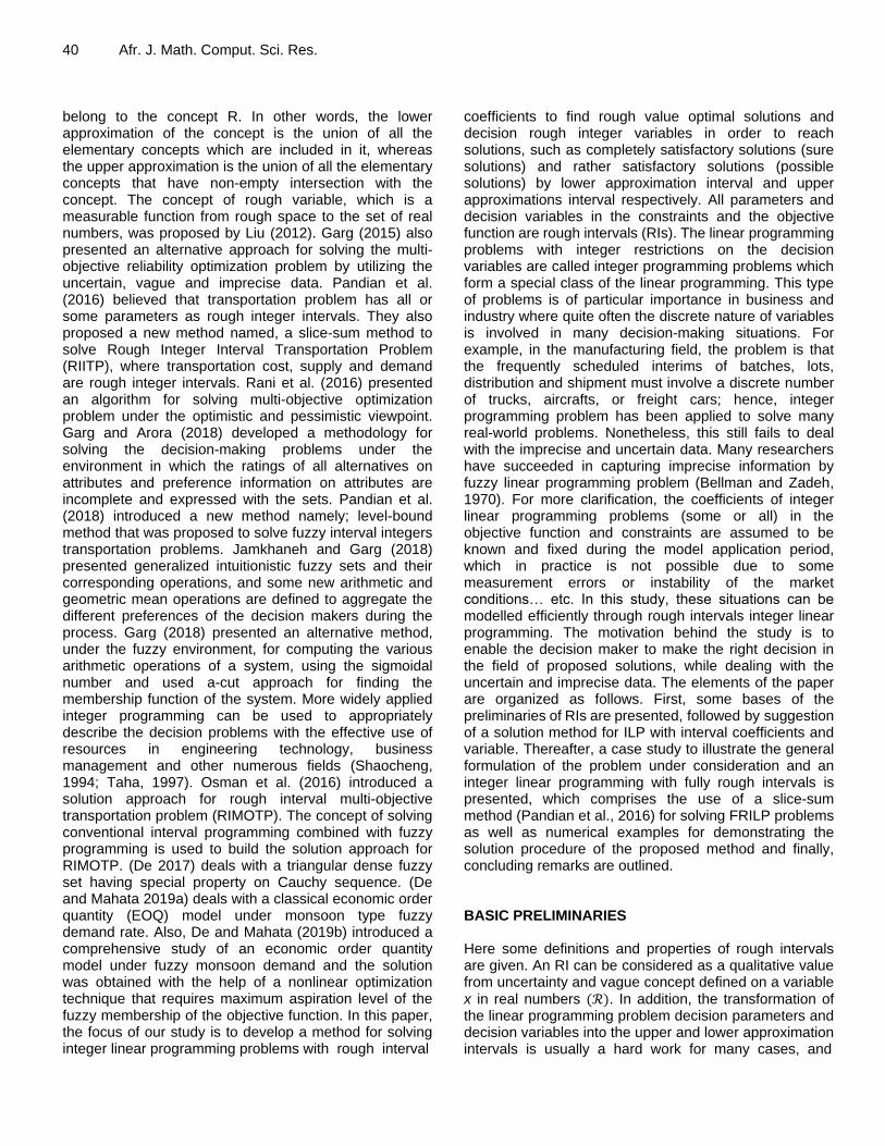
40 Afr. J. Math. Comput. Sci. Res. belong to the concept R. In other words, the lower approximation of the concept is the union of all the elementary concepts which are included in it, whereas the upper approximation is the union of all the elementary concepts that have non-empty intersection with the concept. The concept of rough variable, which is a measurable function from rough space to the set of real numbers, was proposed by Liu (2012). Garg (2015) also presented an alternative approach for solving the multi-objective reliability optimization problem by utilizing the uncertain, vague and imprecise data. Pandian et al. (2016) believed that transportation problem has all or some parameters as rough integer intervals. They also proposed a new method named, a slice-sum method to solve Rough Integer Interval Transportation Problem (RIITP), where transportation cost, supply and demand are rough integer intervals. Rani et al. (2016) presented an algorithm for solving multi-objective optimization problem under the optimistic and pessimistic viewpoint. Garg and Arora (2018) developed a methodology for solving the decision-making problems under the environment in which the ratings of all alternatives on attributes and preference information on attributes are incomplete and expressed with the sets. Pandian et al. (2018) introduced a new method namely; level-bound method that was proposed to solve fuzzy interval integers transportation problems. Jamkhaneh and Garg (2018) presented generalized intuitionistic fuzzy sets and their corresponding operations, and some new arithmetic and geometric mean operations are defined to aggregate the different preferences of the decision makers during the process. Garg (2018) presented an alternative method, under the fuzzy environment, for computing the various arithmetic operations of a system, using the sigmoidal number and used a-cut approach for finding the membership function of the system. More widely applied integer programming can be used to appropriately describe the decision problems with the effective use of resources in engineering technology, business management and other numerous fields (Shaocheng, 1994; Taha, 1997). Osman et al. (2016) introduced a solution approach for rough interval multi-objective transportation problem (RIMOTP). The concept of solving conventional interval programming combined with fuzzy programming is used to build the solution approach for RIMOTP. (De 2017) deals with a triangular dense fuzzy set having special property on Cauchy sequence. (De and Mahata 2019a) deals with a classical economic order quantity (EOQ) model under monsoon type fuzzy demand rate. Also, De and Mahata (2019b) introduced a comprehensive study of an economic order quantity model under fuzzy monsoon demand and the solution was obtained with the help of a nonlinear optimization technique that requires maximum aspiration level of the fuzzy membership of the objective function. In this paper, the focus of our study is to develop a method for solving integer linear programming problems with rough interval

coefficients to find rough value optimal solutions and decision rough integer variables in order to reach solutions, such as completely satisfactory solutions (sure solutions) and rather satisfactory solutions (possible solutions) by lower approximation interval and upper approximations interval respectively. All parameters and decision variables in the constraints and the objective function are rough intervals (RIs). The linear programming problems with integer restrictions on the decision variables are called integer programming problems which form a special class of the linear programming. This type of problems is of particular importance in business and industry where quite often the discrete nature of variables is involved in many decision-making situations. For example, in the manufacturing field, the problem is that the frequently scheduled interims of batches, lots, distribution and shipment must involve a discrete number of trucks, aircrafts, or freight cars; hence, integer programming problem has been applied to solve many real-world problems. Nonetheless, this still fails to deal with the imprecise and uncertain data. Many researchers have succeeded in capturing imprecise information by fuzzy linear programming problem (Bellman and Zadeh, 1970). For more clarification, the coefficients of integer linear programming problems (some or all) in the objective function and constraints are assumed to be known and fixed during the model application period, which in practice is not possible due to some measurement errors or instability of the market conditions… etc. In this study, these situations can be modelled efficiently through rough intervals integer linear programming. The motivation behind the study is to enable the decision maker to make the right decision in the field of proposed solutions, while dealing with the uncertain and imprecise data. The elements of the paper are organized as follows. First, some bases of the preliminaries of RIs are presented, followed by suggestion of a solution method for ILP with interval coefficients and variable. Thereafter, a case study to illustrate the general formulation of the problem under consideration and an integer linear programming with fully rough intervals is presented, which comprises the use of a slice-sum method (Pandian et al., 2016) for solving FRILP problems as well as numerical examples for demonstrating the solution procedure of the proposed method and finally, concluding remarks are outlined. BASIC PRELIMINARIES Here some definitions and properties of rough intervals are given. An RI can be considered as a qualitative value from uncertainty and vague concept defined on a variable

x in real numbers . In addition, the transformation of the linear programming problem decision parameters and decision variables into the upper and lower approximation intervals is usually a hard work for many cases, and

conversion process needs the following definitions to be known. Further details are found in Hamazehee et al. (2014) and Rebolledo (2006):

Definition 1

''The qualitative value is called a rough interval (RI) when two closed intervals are assigned:

and on to where

.Moreover,

1. If then A surely takes 2. If 3. If

are called the lower approximation interval (LAI) and the upper approximation interval (UAI)

of , respectively. Moreover, is denoted by = ( ).

Also, the intervals and are not the complement of each other" (Hamazehee et al., 2014).

Note: We can symbolize [ ] and [ ] where LL, UL, LU, and UU represent lower lower, upper lower, lower upper, upper upper respectively.

Example 1

If A is the concept of “Hot” as the qualitative value defined on a temperature variable x in R, one may consider:

[[ ] [ ]]

Then, by Definition 1, the temperature variable x surely takes a value between 25 and 45°C. Similarly, x possibly takes a value between 15 and 65°C. Note that, common

sense and general knowledge can help define and . For instance: – The temperature of the human body is about 37°C; any warmer temperature would not be considered “Cold”. – On average, a human hand cannot hold an object, whose temperature is over 65°C, because it is “Hot”. – If something is colder than the environment (let us say 15°C, it cannot be considered “Warm” anymore.

Definition 2

''The arithmetic operations on RIs are depending on interval arithmetic, so we will state some of these arithmetic operations as follows'' (Rebolledo, 2006):

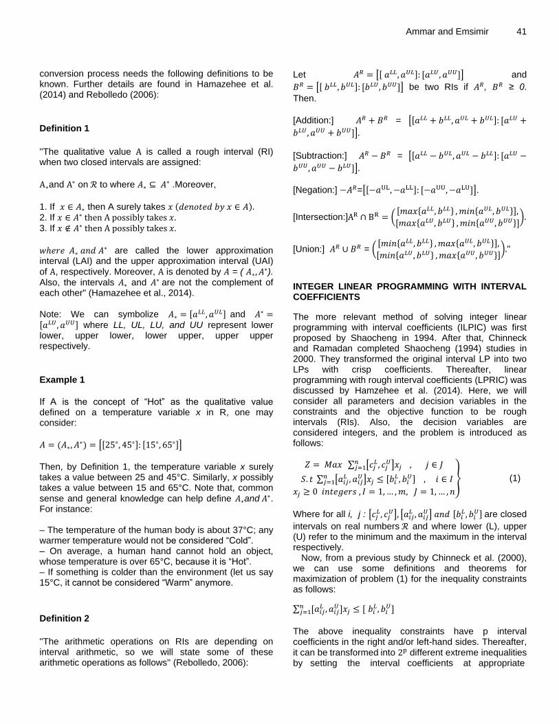
Ammar and Emsimir 41

Let [[ ] [ ]] and

[[ ] [ ]] be two RIs if , ≥ 0.

Then.

[Addition:] = [[ ] [

]]

[Subtraction:] = [[ ] [

]]

[Negation:] =[[ ] [ ]].

[Intersection:] ([ { } { }]

[ { } { }])

[Union:] = ([ { } { }]

[ { } { }]) ''

INTEGER LINEAR PROGRAMMING WITH INTERVAL COEFFICIENTS

The more relevant method of solving integer linear programming with interval coefficients (ILPIC) was first proposed by Shaocheng in 1994. After that, Chinneck and Ramadan completed Shaocheng (1994) studies in 2000. They transformed the original interval LP into two LPs with crisp coefficients. Thereafter, linear programming with rough interval coefficients (LPRIC) was discussed by Hamzehee et al. (2014). Here, we will consider all parameters and decision variables in the constraints and the objective function to be rough intervals (RIs). Also, the decision variables are considered integers, and the problem is introduced as follows:

∑ [

]

∑ [

] [

]

} (1)

Where for all i, j : [

] [

] [

] are closed

intervals on real numbers and where lower (L), upper (U) refer to the minimum and the maximum in the interval respectively.

Now, from a previous study by Chinneck et al. (2000), we can use some definitions and theorems for maximization of problem (1) for the inequality constraints as follows:

∑ [

] [

]

The above inequality constraints have p interval coefficients in the right and/or left-hand sides. Thereafter, it can be transformed into different extreme inequalities by setting the interval coefficients at appropriate

42 Afr. J. Math. Comput. Sci. Res.

Table 1. Production data for an example 2.

Product Required production time in department (h/unit)

Seasonal profit ($/unit) 1 2 3

A [3,5] [2,4] [1,2] [1,3]

B [2,4] [1,3] [3,5] [2,4]

Available time [550,700] [380,500] [200,300] -

combinations of the bounding values on the coefficient ranges", such as in inequality constraints where P =2,

. Let be the set of all solutions for the extreme inequality. Then:

⋃ and ⋂

Definition 3

''For inequality constraints, if there exists one extreme

inequality that its solution set is the same as ( ), then it is called the maximum value range (minimum value range) inequality'' (Hamazehee et al., 2014). Theorem 3a Consider inequality constraints, where

Then, ∑

and ∑

be the

minimum value range and maximum value range inequalities, respectively (Hamazehee et al., 2014). Theorem 3b Consider ILPIC problem (1) (Hamazehee et al., 2014).

Then, for any given feasible solution , we have: ∑

∑

for all

Definition 4

''For a given feasible solution of ILPIC Problem

(1), the value ∑

∑

is called the most

suitable value (the least suitable value) of the objective function'' (Hamazehee et al., 2014).

From the above Theorems 1 and 2 and the Definitions 3 and 4, we can find the best and worst optimal solutions of the ILPIC Problem (1). By transforming the original ILPIC problem (1) into two classical ILP problems, we

can call them and . (1) The best optimal solution is found by solving:

∑

∑

} (2)

(2) The worst optimal solution is found by solving:

∑

∑

} (3)

Briefly, and used the greatest and the smallest suitable value of the objective function and the maximum (minimum) value range inequalities of problem (1).

Note that, there are 3 possible outcomes for ILPIC problem (1) as follows:

- If and have optimal solutions, then ILPIC problem (1) has a finite bounded optimal range.

- If is unbounded then ILPIC problem (1) is unbounded.

- If is infeasible then ILPIC problem (1) is infeasible. More clarification and proof can be found in Hamazehee et al. (2014). Example 2. A company produces two sorts of products, A and B, and three departments 1, 2 and 3 are assigned to produce them. Each product takes a time to be produced by the three departments; the following Table 1 shows the details.

Thereafter, the model of this optimization problem can be formulated as follows:

ILPIC = [ ] [ ] [ ] [ ] [ ] [ ] [ ] [ ] [ ] [ ] [ ]

Here, the optimal range of ILPI for Example 2 can be obtained by solving two classical ILPs as follows: The best optimal solution

Ammar and Emsimir 43

Table 2. The first plan.

Product Required production time in department (h/unit) Seasonal profit

($/unit) 1 2 3

A [3,4] [2,4] [1,2] [2,3]

B [2,4] [3,4] [3,5] [2,3]

Available time [600,650] [400,450] [200,300] -

Table 3. The second plan.

Product Required production time in department (h/unit)

Seasonal profit ($/unit) 1 2 3

A [2,4] [2,3] [1,3] [2,4]

B [2,3] [2,4] [3,4] [2,3]

Available time [550,700] [380,500] [230,260] -

and The worst optimal solution

We then apply the branch and bound to Example 2 to

find integer optimal solutions.

[ ] [ ] [ ]

INTEGER LINEAR PROGRAMMING WITH FULLY ROUGH INTERVALS

In this part, we consider the linear programming problems with rough interval coefficients and variables (ILPFRI).

Formulating linear programming model requires that specific values be chosen for the model coefficients. However, the values of many of these coefficients are only approximately known. For instance, the Director of the company wishes to know the range of optimal solutions that could be returned by an ILP model with uncertain coefficients. On the other hand, the manager may put some plans or ask the opinions of some experts to determine the uncertain coefficients. Now, we will give a case study to clarifying the idea. Case study A company produces two sorts of products, A and B, and three departments 1, 2 and 3 are required to produce them. Each product takes a time to be produced by the three departments. Production experts put three plans for production due to the uncertainty of parameters. Each plan gives the approximate production time of each product in the 3 departments and seasonal profit of each product as shown in Tables 2, 3 and 4, e.g. the required production time for product A in Department 1 due to the first plan is between 3 and 4 h per unit and its seasonal profit is between $2 and $3 per unit with hours of production time available in the three departments.

The production experts would like to allocate the production capacity so that it not only finds the optimal product mixture but also use the three plans together. In order to solve this problem, the parameters should be determined. Since the parameters are given by the three plans, one way to involve all plans is representing the parameters by rough interval. In Table 5, the upper and lower approximations of rough interval coefficients are computed based on the union and intersection of the plans.

Now, in the case study, let and denote the respective amounts of products 1 and 2 which should be produced. Then, the model of this optimization problem can be formulated in Example 3 as follows:

𝑳𝑷𝑭𝑹𝑰 = ([ ], [ 𝑈 ]) = Max [[2,3]: [1,4]] ⨂[[ 1

, 1𝑈 ]: [ 1

𝑈 , 1𝑈𝑈 ]]⨁

[[2,3]: [2,4]] ⊗ [[ 2 , 2

𝑈 ]: [ 2 𝑈 , 2

𝑈𝑈 ]]

S.t [[ 3,4]: [2,5]] ⨂[[ 1

, 1𝑈 ]: [ 1

𝑈 , 1𝑈𝑈 ]]⨁[[2,3]: [2,4]]

⨂[[ 2 , 2

𝑈 ]: [ 2 𝑈 , 2

𝑈𝑈 ]] [[600,650]: [550,700]]

44 Afr. J. Math. Comput. Sci. Res.

Table 4. The third plan.

Product Required production time in department (h/unit) Seasonal profit

($/unit) 1 2 3

A [3,5] [2,4] [1,2] [1,3]

B [2,4] [1,3] [3,5] [2,4]

Available time [550,700] [380,500] [200,300] -

Table 5. The coefficients of the problem.

Product Required production time in department (h/unit) Seasonal profit

($/unit) 1 2 3

A ([3,4]: [2,5]) ([2,3]: [2,4]) ([1,2]: [1,3]) ([2,3]: [1,4])

B ([2,3]: [2,4]) ([3,3]: [1,4]) ([3,4]: [3,5]) ([2,3]: [2,4])

Available time ([600,650]: [550,700]) ([400,450]: [380,500]) ([230,260]: [200,300]) -

[[ ] [ ]] ⨂[[

] [

]]⨁[[ ] [ ]]

⨂[[

] [

]] [[ ] [ ]]

[[ ] [ ]] ⨂[[

] [

]]⨁[[ ] [ ]]

⨂[[

] [

]] [[ ] [ ]]

{

}

Example 3 may involve other constraints and variables, in other words, the constraints can be of the form ≤, ≥ or =. Also, variables can be sign-restricted (x ≤ 0 or x ≥ 0) or unrestricted in sign.

This study will be limited to the variables which are sign-restricted

as

.

Problem formulation The general formula of the integer linear programming problem with fully rough interval for coefficients and variables (ILPFRI) may be presented as:

(14)

Where

[[

] [

]] , [[

] [

]]

[[

] [

]] [[

] [

]]

are rough interval coefficients and variables of the objective function and the constraints. Also, let denote the vector of all decision variables.

Remark 1: According to rough interval properties introduced earlier, we have

[

] [

]

,

[

] [

]

[

] [

]

[

] [

]

,

Definition 5 In problem (4), we can define the following sets:

|∑

|∑

|∑

|∑

Where ( .

Note: for the sets we have: (Hamazehee et al., 2014). Definition 6 Consider all of the corresponding ILPFRI problems and LP of problem (4) (Atteya, 2016; Bazaraa, 2010).

a) The interval [ ] [ ] is called the surely

(possibly) optimal range symbolized [ ] [ ] of problem (4), if the optimal range of each (ILPFRI) is a superset (subset) of

[ ] [ ] b) Let [ ] [ ] be surely (possibly) optimal range of the problem (4). Then the rough interval

[[ ]: [ 𝑈 ]] = 𝑴𝒂𝒙 ∑ [[ ,

𝑈 ]: [ 𝑈 ,

𝑈𝑈 ]] =1 ⨂ [[

, 𝑈 ]: [

𝑈 , 𝑈𝑈 ]]

∑ ∑ [[

, 𝑈 ]: [

𝑈 , 𝑈𝑈 ]]

=1 ⨂[[ ,

𝑈 ]: [ 𝑈 ,

𝑈𝑈 ]]𝒎𝒊=𝟏

[[ ,

𝑈 ]: [ 𝑈 ,

𝑈𝑈 ]]}

,

𝑈 , 𝑈 ,

𝑈𝑈 0 , ,

(4)

[[ ] [ ]] is called the rough optimal range of

problem (4); also any point, optimal value belongs to

[ ] [ ] and is called a completely (rather) satisfactory solution of the problem (4). c) A solution is surely-feasible, iff it belongs to the lower approximation of the feasible set. d) A solution is possibly -feasible, iff it belongs to the upper approximation of the feasible set. e) A solution is surely-not feasible, iff it does not belong to the upper approximation of the feasible set. Solution procedures In order to solve problem (4), we will construct two integers linear programming (ILP) problems with interval coefficients and variables. One of these problems is an ILP problem where all of its coefficients are upper approximations interval (UAI) of rough intervals and represents rather satisfactory solutions, while the other is an ILP problem where all of its coefficients are lower approximations interval (LAI) of rough intervals and represents complete solutions. Then the two ILP problems are sliced into four crisp problems through the following steps.

Step 1: Find the possibly optimal range solution [ ] by solving the upper approximation interval of problem (4).

∑ [

]⨂[

]

∑ ∑ [

]⨂[

] [

]

(5)

Step 2: Find the surly optimal range solution

[ ] by solving the lower approximation of problem (4).

∑ [

]⨂[

]

∑ ∑ [

]⨂[

] [

]

(6)

Step 3: According to Definition 6, the possibly optimal range

solution of problem (5) can be obtained by slicing it into two classical ILPs as follows:

∑

∑

and

∑

∑

Ammar and Emsimir 45 By Definition 5, the feasible solution set of problems (7) and (8) is

equivalent to . Thus, the interval [ ] is the optimal possible solution range of problem (5).

We can see that the interval [ ] is equivalent to the possibly optimal range of problem (4). Toward this end, since problem (1) is an arbitrary corresponding LPIC problem of (4), we have

[

] [

] [

] [

]

[

] [

] [

] [

]

[

] [

] [

] [

]

[

] [

] [

] [

]

Step 4: The surly optimal range solution of problem (6) can be obtained by solving two classical LPs as:

∑

∑

and

∑

∑

(10)

By Definition 5, the feasible solution set of problems (9) and (10) is

equivalent to . Thus, the interval [ ] is the optimal solution range of problem (6). Also, the

interval [ ] is the optimal possible solution range for

problem (5) and the interval [ ] is the sure solution range (6).

Where the rough value optimal solutions and decision

rough integer variables in problem (4) will be as:

[[ ] [ ]],

[[

] [

]],

.

Where the possibly optimal values range solutions for [ ].

Also, the surely optimal values range solutions for [ ] In addition, [

] is the integer completely

satisfactory solutions, and [

] is integer rather satisfactory

solutions. Now, a relation has been established between optimal solutions

of the integer linear programming problem with fully rough interval

in problem (4) and four problems , problems (7), (8), (9) and (10) respectively. The established relation is used in the proposed method, slice-sum method.

Theorem 4

If the set { } is an optimal solution for the or

46 Afr. J. Math. Comput. Sci. Res. (7) problem of the problem (ILPFRI) or (4) with the maximum

optimal value for , the set { } is an optimal

solution for the or (10) problem of the problem (ILPFRI) or

(4) with the maximum optimal value for , the set

{ } is an optimal solution for the or (9) problem

of the problem (ILPFRI) or (4) with the maximum optimal value for

, and the set { } is an optimal solution for the

or (8) problem of the problem (ILPFRI) or (4) with the

maximum optimal value for , then the set of rough integer

intervals {( [

] [

]) } is an optimal

solution for the problem (4) with maximum optimal values

([ ] [ ]) provided

Now, since {

} { } {

} { } are optimal solutions for the problems

,respectively and

then we can conclude that the set of rough integer

intervals {( [

] [

]) } is a feasible solution

to the problem (4).

Let {( [

] [

]) } be a feasible

solution to the problem (4).

Therefore, { } {

} {

} { } are feasible solutions to the problems

respectively.

Since { } {

} {

} { } are feasible solutions to the problems

respectively. We have:

∑

∑

∑

∑

∑

∑

∑

∑

This implies that [ ] [ ]

∑ [

] [

] ⨂ [

] [

]

∑([

] [

]) ⊗

𝒎

𝟏

([

] [

])

∑([

] [

])

𝒎

𝟏

⊗([

] [

])

Therefore, the set of rough integer intervals

{( [

] [

]) } is an optimal solution for the

problem (4) with maximum optimal values ([ ] [ ]).

Hence, the theorem is proved (Pandian et al., 2016). Figure 1 shows flowchart of the solution steps, which was provided for more clarification.

To solve the problem indicated in the case study, we should solve two integer linear programming fully interval problems ILPFI =

[ ] as follows:

[ ] [ ] ⨂ [

] ⨁ [ ]⨂[

]

Subject to [ ] ⨂ [

] ⨁ [ ]⨂ [

]

[ ]

[ ] ⨂[

] ⨁ [ ]⨂[

] [ ] [ ]⨂[

] ⨁ [ ]⨂[

]

[ ]

[ ] [ ] ⨂ [

]⨁ [ ]⨂ [

]

Subject to [ ]⨂ [

]⨁ [ ]⨂ [

]

[ ]

[ ]⨂ [

] ⨁ [ ] ⨂ [

] [ ]

[ ]⨂ [

] ⨁ [ ] ⨂[

] [ ]

- In the ILPFI Problem, ( ) is transformed to ILP problems

and where their feasible sets are , respectively.

- In the ILPFI Problem, ( ) is transformed to ILP problems

and , where their feasible sets are respectively.

max

S.t

max

S.t

Ammar and Emsimir 47

Figure 1. Flowchart of the proposed approach for solving fully rough integer linear programming problems.

Table 6. Optimal values and solutions of ILP programs in the case study.

Problem 𝑰𝑳𝑷𝑳 𝑰𝑳𝑷𝑳𝑳 𝑰𝑳𝑷 𝑳 𝑰𝑳𝑷

Optimal values 66 230 660 1040

𝒙𝟏 𝑹 66 115 210 240

𝒙 𝑹 0 0 10 20

max

S.t

max

S.t

We used ''WinQSB'' program (Olga et al., 2009) to find rough value

optimal solutions and decision rough integer variables

and apply branch and bound algorithm (Gupta and Mohan, 2006) to find integer optimal solutions for the case study as shown in Table

6. Optimal values and solutions of ILP programs in the case study are presented in Table 6. Here the integer rough optimal solutions is

[[ ] [ ]]

[[ ] [ ]].

The rough optimal values range solutions for

[[ ] [ ]] [[ ] [ ]].

Where the possibly optimal values range solutions for [ ] [ ]

Also, the surely optimal values range solutions for [ ] [ ]. In addition, [

] [ ] [

] [ ] is integer completely

satisfactory solutions and [

] [ ] [

] [ ] is integer rather satisfactory solutions.

We think that this is the way to the solution, where the director of

48 Afr. J. Math. Comput. Sci. Res. the company has put all the possible solutions to avoid the economic crises and market fluctuations (the uncertainty of parameters). Example 3 Consider the following ILPFRI problem as follows:

[[ ] [ ]]

[ ] [ ] ⊗ ⨁ [ ] [ ] ⊗

⨁ [ ] [ ] ⊗

⨁ [ ] [ ] ⊗

[ ] [ ] ⊗ ⨁ [ ] [ ] ⊗

}

Subject to

{

[ ] [ ]⨂

⨁ [ ] [ ] ⨂ ⨁

[ ] [ ] ⨂ ⨁ [ ] [ ] ⨂

[ ] [ ] ⨂ ⨁ [ ] [ ] ⨂

[ ] [ ]

{ [ ] [ ] ⨂

⨁ [ ] [ ] ⊗

[ ] [ ] }

{ [ ] [ ] ⨂

⨁ [ ] [ ] ⨂

[ ] [ ] }

{[ ] [ ] ⨂

⨁ [ ] [ ] ⨂

[ ] [ ] }

{

}

Where

[

] [

] ,

[

] [

]

[

] [

] ,

[

] [

]

[

] [

] and

[

] [

]

In order to solve problem (Example 3), we will solve two ILPFI problems as follows:

[ ]⨂[

]⨁ [ ]⨂[

]

⨁ [ ] ⨂[

]⨁[ ]⨂[

]

⨁[ ]⨂[

]⨁[ ]⨂[

]

}

Subject to

[ ]⨂[

]⨁[ ]⨂[

]⨁[ ]

⨂[

]⨁[ ]⨂[

]⨁[ ] ⊗

[

]⨁[ ]⨂[

] [ ]

}

{[ ]⨂[

]⨁[ ]⨂[

]

[ ]}

{[ ]⨂[

]⨁[ ] ⨂[

]

[ ]}

{[ ]⨂[

]⨁[ ]⨂[

]

[ ]}

{

}

and

[ ]⨂[

]⨁[ ]⨂[

]

⨁[ ]⨂[

]⨁[ ]⨂[

]

⨁[ ]⨂[

]⨁[ ]⨂[

]

}

Subject to

[ ]⨂[

]⨁[ ]⨂[

]⨁[ ]

⨂[

]⨁[ ]⨂ [

]⨁[ ]⨂

[

]⨁[ ]⨂[

] [ ]

}

{[ ] ⨂ [

]⨁[ ] ⨂ [

]

[ ]}

{[ ]⨂[

]⨁[ ]⨂[

]

[ ]}

{[ ]⨂[

]⨁[ ]⨂[

]

[ ] }

{

}

According to Solution Procedures, the optimal range of ILPIC

Problems and can be obtained by solving four classical LPs as follows:

Subject to

And

Subject to

Subject to

Table 7. Optimal values and solutions of Example 3.

Problem 𝑰𝑳𝑷𝑳 𝑰𝑳𝑷𝑳𝑳 𝑰𝑳𝑷 𝑳 𝑰𝑳𝑷

Optimal values 14 46 328 1065

𝒙𝟏 𝑹 1 2 8 30

𝒙 𝑹 0 0 0 0

𝒙 𝑹 0 0 0 0

𝒙 𝑹 1 4 10 15

𝒙 𝑹 1 2 8 15

𝒙 𝑹 0 0 0 0

Subject to

To find rough value optimal solutions decision rough integer

variables and apply branch and bound algorithm (Gupta and

Mohan, 2006) to find integer optimal solutions of Example 3 as shown in Table 7.

The possibly optimal values range solutions for

[ ] [ ]

the surely optimal values range solutions for

[ ] [ ] in addition, the rough optimal values range solutions ILPRI

[ ] [ ] [[ ] [ ]] Where [

] [ ] [

] [ ],

[

] [ ] [

] [ ] [

] [ ] [

] [ ].

Are the integers completely satisfactory solutions. And

[

] [ ] [

] [ ] [

] [ ] [

] [ ]

[

] [ ] [

] [ ]

are the integers’ rather satisfactory solutions. Also,

[ ] [ ]

[ ] [ ]

[ ] [ ]

[ ] [ ]

[ ] [ ]

[ ] [ ] . are the integers rough optimal solutions.

Note that, decision variables and the optimal values are rough

Ammar and Emsimir 49 intervals. Thus, we have completely satisfactory solutions and rather satisfactory solutions. Then, we give the decision maker more freedom to choose.

DISCUSSION Comparing the linear programming with rough Interval coefficients by Hamazehee et al. (2014), who only used the rough interval with coefficients in linear programming problems, and with fuzzy interval integer transportation problems by Pandian et al. (2018), who used a new method namely; level-bound method that was proposed to solve fuzzy interval integers transportation problems, this study used fully rough intervals integer linear programming problems, where all parameters and decision variables in the constraints and the objective function are rough intervals, since many linear programming problems in our real life require that the decision variables be integers. In addition, rough intervals are very important to tackle the uncertainty and imprecise data in decision making problems. Moreover, the proposed algorithm enables us to search for the optimal solution in the largest range of possible solutions. Furthermore, N suggested solutions are obtained to enable the decision maker to choose the best decisions. On the other hand, some solutions, such as completely satisfactory solutions (surely solutions) as in problem (6) (step 2), are successfully reached, which lets us be sure that the optimal solution is in the lower approximation interval. While the rather satisfactory solutions (possible solutions), as in problem (5) (step 1), makes it possible that the optimal solution is in the upper approximation interval. The slice-sum method can be served as an important tool for the decision makers, when they are handling various types of logistic problems with rough variable parameters. Furthermore, the branch and bound technique is used to reach the integer programming. The results, in the form of rough intervals method, do not ignore any part of the solution area. The motivation behind the study is to enable the decision maker to make the right decision in the field of proposed solutions, in case of having to deal with the uncertainty and imprecise data. Finally, to clarify the idea and support this paper, some examples are solved by "WinQSB" program (Olga et al., 2009) in order to illustrate the new concepts. Conclusion Some basic concepts of rough intervals are reviewed in this research paper. Then we presented a methodology for solving fully rough integer linear programming problems and found rough value optimal solutions and decision rough integer variables, where all parameters and decision variables in the constraints and the objective functions are rough intervals. The proposed model depends on slice-sum method, branch and bound

50 Afr. J. Math. Comput. Sci. Res. method and integer programming, which is a good technique for many LP problems which require that the decision variables are integers. Also, the used rough intervals are very important to tackle the uncertainty in decision making problems. In addition, we obtained N suggested solutions in order to enable the decision maker to take the best decision. Furthermore, we got on solutions such as completely satisfactory solutions (surely solutions) and rather satisfactory solutions (possibly solutions) by lower approximation interval and upper approximations interval respectively. The results are in the form of intervals and the interval method does not ignore any part of solution area. It is thought that the rough intervals are useful new tools to tackle the uncertainty, vague and imprecise data in decision making problems. Also, a flowchart of the steps to solve the problem is provided for more clarification. CONFLICT OF INTERESTS The authors have not declared any conflict of interests. REFERENCES Atteya T (2016) Rough multiple objective programming. European

Journal of the Operational Research 248(1):204-210. Bazaraa M, Jarvis J, Sherali H (2010). Linear programming and network

flows. John Wiley and Son, New York. Bellman R, Zadeh L (1970). Decision making in fuzzy environment.

Management science 17(4):B-141. Chinneck J, Ramadan K (2000). Linear programming with interval

coefficients. Journal of the Operational Research Society 51(2):209-220.

De SK (2019). Triangular dense fuzzy lock sets. Soft Computing 22(21):7243-7254. DOI 10.1007/s00500-017-2726-0.

De SK, Mahata G (2019a). A cloudy fuzzy economic order quantity

model for imperfect‑quality items with allowable proportionate discounts. Journal of Industrial Engineering International 15(4):571-583. https://doi.org/10.1007/s40092-019-0310-1.

De SK, Mahata G (2019b). A comprehensive study of an economic order quantity model under fuzzy monsoon demand. Sadhana 44(4):89. https://doi.org/10.1007/s12046-019-1059-3.

Garg H (2015). Multi-objective optimization problem of system reliability under intuitionistic fuzzy set environment using Cuckoo Search algorithm. Journal of intelligent and fuzzy systems 29(4):1653-1669.

Garg H (2018). Some arithmetic operations on the generalized sigmoidal fuzzy numbers and its application. Granular computing 3(1):9-25.

Garg H, Arora R (2018). A nonlinear-programming methodology for

multi-attribute decision-making problem with interval-valued intuitionistic fuzzy soft sets information. Applied Intelligence 48(8):2031-2046.

Gupta PK, Mohan M (2006). Problems in Operations Research, Sultan Chand and Sons, New Delhi.

Hamazehee A, Yaghoobi M, Mashinchi M (2014). "Linear Programming with Rough Interval Coefficients". Journal of Intelligent and Fuzzy Systems 26(3):1179-1189.

Jamkhaneh B, Garg H (2018). Some new operations over the generalized intuitionistic fuzzy sets and their application to decision-making process. Granular computing 3(2):111-122.

Liu B (2012). Theory and Practice of Uncertain Programming (Vol. 239). Berlin: Springer.

Olga IA, Doina F, Gheorghe P, Codruta OH (2009). ''WinQSB'' simulation software - a tool for professional development. Science Direct 1(4):2786-2790.

Osman S, El-Sherbiny M, Khalifa A, Farag H (2016). A Fuzzy Technique for Solving Rough Interval Multiobjective Transportation Problem. International Journal of Computer Applications 147(10):49-57.

Pandian P, Natarajan G, Akilbasha A (2016) "Fully Rough Integer Interval Transportation Problems". International Journal of Pharmacy and Technology 8(2):13866-13876.

Pandian P, Natarajan G, Akilbasha A (2018) Fuzzy interval integer transportation problems. International Journal of Pure and Applied Mathematics 119 (9):133-142.

Pawlak Z, Skowron A (2007). Rudiment of rough sets, Information Sciences 177(1):3-27.

Rani D, Gulati T, Garg H (2016) Multi-objective non-linear programming problem in intuitionistic fuzzy environment: Optimistic and pessimistic view point. Expert Systems with Applications 64(1):228-238.

Rebolledo M (2006). Rough intervals-enhancing intervals for qualitative modeling of technical systems Artificial Intelligence 170(8-9):667-685.

Shaocheng T (1994). Interval number and fuzzy number linear programming, Fuzzy Sets and Systems 66(3):301-306.

Taha H (1997). "Operation Research-An Introduction", 6th Edition. Mac Milan Publishing Co, New York.