A Mathematical Model for Quorum Sensing in …keener/pubs/papers/bulm0205.pdf · A Mathematical...

Available online at http://www.idealibrary.com ondoi:10.1006/bulm.2000.0205Bulletin of Mathematical Biology (2000) 00, 1–22

A Mathematical Model for Quorum Sensing inPseudomonas aeruginosa

JACK D. DOCKERY∗

Department of Mathematics,Montana State University,Bozeman,MT 59718, U.S.A.E-mail: [email protected]

JAMES P. KEENERDepartment of Mathematics,University of Utah,Salt Lake City,UT 84112, U.S.A.E-mail: [email protected]

The bacteria Pseudomonas aeruginosa use the size and density of their colonies toregulate the production of a large variety of substances, including toxins. This phe-nomenon, called quorum sensing, apparently enables colonies to grow to sufficientsize undetected by the immune system of the host organism.In this paper, we present a mathematical model of quorum sensing in P. aeruginosathat is based on the known biochemistry of regulation of the autoinducer that is cru-cial to this signalling mechanism. Using this model we show that quorum sensingworks because of a biochemical switch between two stable steady solutions, onewith low levels of autoinducer and one with high levels of autoinducer.

c© 2000 Society for Mathematical Biology

1. INTRODUCTION

The bacterium Pseudomonas aeruginosa is an increasingly prevalent humanpathogen, responsible for 12% of hospital-acquired urinary tract infections, 10%of blood stream infections, and 8% of surgical wound infections. It is also one ofthe most common and lethal pathogens responsible for ventilator-associated pneu-monia in intubated patients, with directly attributable deaths reaching 38%. Cysticfibrosis patients are characteristically susceptible to chronic infection by P. aerug-inosa, which is responsible for high rates of illness and death in this population(Van Delden and Iglewski, 1998). Author:

Van Delden and Iglewski(1998) OK? or VanDelden et al. please check

The ability of P. aeruginosa to invade a potential host relies largely on its abilityto control many of its virulence factors by a mechanism that monitors cell density

∗Author to whom correspondence should be addressed.

0092-8240/00/000001 + 22 $35.00/0 c© 2000 Society for Mathematical Biology

2 J. D. Dockery and J. P. Keener

and allows communication between bacteria. That is, isolated production of extra-cellular virulence factors by a small number of bacteria would probably lead to anefficient host response neutralizing these factors. However, the typical behavior isfor virulence factors to be expressed by an entire colony only after the colony hasachieved a certain size or density. In this way, cells excrete extracellular virulencefactors only when they can be produced at high enough levels to overcome hostdefenses.

Another feature of persistent P. aeruginosa infections in cystic fibrosis patients isthat when cell densities are high enough, the population as a whole begins to pro-duce copious amounts of exopolysaccharide alginate (Govan and Deretic, 1996). ItAuthor:

Govan and Deretic (1996)OK?

is thought that these bacteria grow inside a biofilm [defined as micro-colonies sur-rounded by an exopolysaccharide, see Characklis and Marshall (1990)] as a sur-Author:

Characklis and Marshall(1990) OK?

vival strategy since the surrounding polymer matrix protects bacteria. P. aerugi-nosa growing in an alginate ‘slime matrix’ are resistant to antibiotics and disinfec-tants (Govan and Deretic, 1996).

Recently, a cell-to-cell signaling system has been shown to be involved in thedifferentiation of P. aeruginosa biofilms (Davies et al., 1998). A mutant defectivein the production of a certain signaling molecule formed an abnormal biofilm thatin contrast to the wild type biofilm was sensitive to low concentrations of the de-tergent sodium dodecyl sulfate (SDS). Furthermore, the addition of the signalingmolecule to the batch culture medium restored production of a slimy biofilm thatwas SDS resistant (Davies et al., 1998).

The ability of cells to sense their own cell density, to communicate with eachother and to behave as a population instead of individually is called quorum sens-ing. Quorum sensing is known to occur in a growing number of examples, includ-ing sporulation and fruiting body formation by Myxococcus xanthus and antibioticproduction by several species of Streptomyces. Perhaps the best characterized ex-ample is in the autoinduction of luminescence in the symbiotic marine bacteriumVibrio fischeri, which colonizes the light organs of certain marine fishes and squids(Fuqua et al., 1996).

In all of these examples the fundamental mechanism of quorum sensing is thesame, although the biochemical details are surprisingly different. These cell-to-cell signaling systems are all composed of a small molecule, called an autoinducer,which is synthesized by an autoinducer synthase, and a transcriptional activatorprotein. The production of the autoinducer is regulated by a specific R-protein. TheR-protein by itself is not active without the corresponding autoinducer, but the R-protein/autoinducer complex binds to specific DNA sequences upstream of the tar-get genes, enhancing their transcription. Thus, at low cell density, the autoinduceris synthesized at basal levels and diffuses into the surrounding medium, where itis diluted. With increasing cell density, however, the intracellular concentration ofthe autoinducer increases until it reaches a threshold concentration beyond whichit is produced autocatalytically, resulting in a dramatic increase of product concen-trations. The autoinducer, therefore, allows the bacteria to communicate with each

A Quorum-Sensing Model 3

other, to sense their own density, and together with a transcriptional activator toexpress specific genes as a population rather than individually.

Quorum sensing is an unusual signaling mechanism for several reasons. First,there are no membrane surface receptors for the signaling molecule, and since theautoinducer is produced on the interior of the cell, the extracellular concentrationof autoinducer is generally smaller than the intracellular concentration. One mighttherefore question how the autoinducer can act as a signal.

The purpose of this paper is to develop and study mathematical models of quo-rum sensing, in order to obtain a deeper understanding of how and when this mech-anism works. We focus on the specific system of P. aeruginosa although the math-ematical principles are the same in other systems. Our emphasis here is on thebiochemical mechanism underlying quorum sensing. In a related study, James etal. (2000) found a simple mathematical model appropriate to V. fischeri that hadmultiple stable steady states and was controlled by extracellular autoinducer. Bycontrast, in Ward et al. (2000), a population dynamics approach was taken for V.fischeri, and switching behavior in which there was cell differentiation was foundas the colony grew in size. The models in both of these studies were systems ofthree first-order, nonlinear, ordinary differential equations. In what follows, weexamine models involving both ordinary and partial differential equations.

2. THE MODEL

The quorum-sensing system of P. aeruginosa is unusual because it has two some-what redundant regulatory systems. The first system described in P. aeruginosawas shown to regulate expression of the elastase LasB and was therefore namedthe las system. The two enzymes, LasB elastase and LasA elastase, are responsi-ble for elastolytic activity which destroys elastin-containing human lung tissue andcauses pulmonary hemorrhages associated with P. aeruginosa infections. The lassystem is composed of lasI, the autoinducer synthase gene responsible for synthesisof the autoinducer 3-oxo-C12-HSL, and the lasR gene that codes for transcriptionalactivator protein. The LasR/3-oxo-C12-HSL dimer, which is the activated form ofLasR, activates a variety of genes, but preferentially promotes lasI activity. Thelas system is positively controlled by both GacA and Vfr, which are needed fortranscription of lasR. The transcription of lasI is also repressed by the inhibitorRsaL.

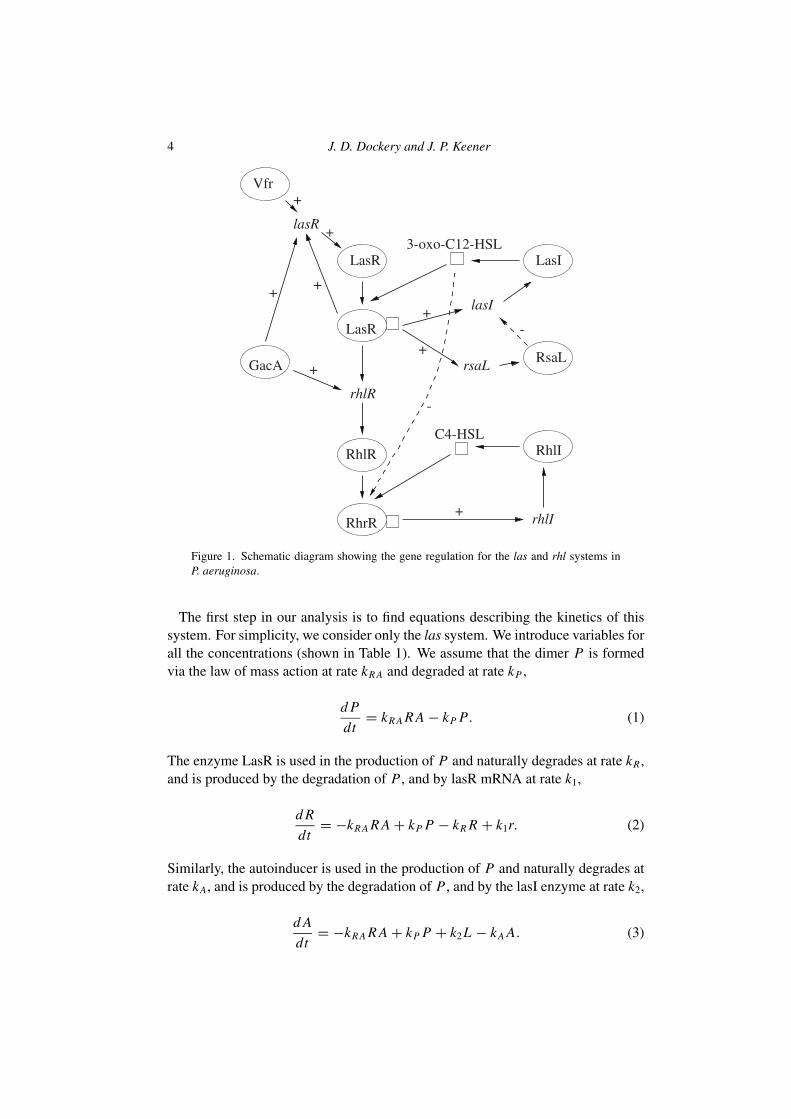
The second quorum-sensing system in P. aeruginosa is named the rhl systembecause of its ability to control the production of rhamnolipid. Rhamnolipid hasa detergent-like structure and is responsible for the degradation of lung surfactantand inhibits the mucociliary transport and ciliary function of human respiratoryepithelium. This system is composed of rhlI, the synthase gene for the autoinducerC4-HSL, and the rhlR gene encoding a transcriptional activator protein. A diagramdepicting these two systems is shown in Fig. 1 (Van Delden and Iglewski, 1998).


lasR

lasI

rhlR

rhlI

+

+

+

+

+

+-

+

+

-

Vfr

LasR

LasR

LasI

RsaLGacA

RhlR

RhrR

RhlIC4-HSL

3-oxo-C12-HSL

rsaL

Figure 1. Schematic diagram showing the gene regulation for the las and rhl systems inP. aeruginosa.

The first step in our analysis is to find equations describing the kinetics of thissystem. For simplicity, we consider only the las system. We introduce variables forall the concentrations (shown in Table 1). We assume that the dimer P is formedvia the law of mass action at rate kR A and degraded at rate kP ,

d P

dt= kR A R A − kP P. (1)

The enzyme LasR is used in the production of P and naturally degrades at rate kR ,and is produced by the degradation of P , and by lasR mRNA at rate k1,

d R

dt= −kR A R A + kP P − kR R + k1r. (2)

Similarly, the autoinducer is used in the production of P and naturally degrades atrate kA, and is produced by the degradation of P , and by the lasI enzyme at rate k2,

d A

dt= −kR A R A + kP P + k2L − kA A. (3)


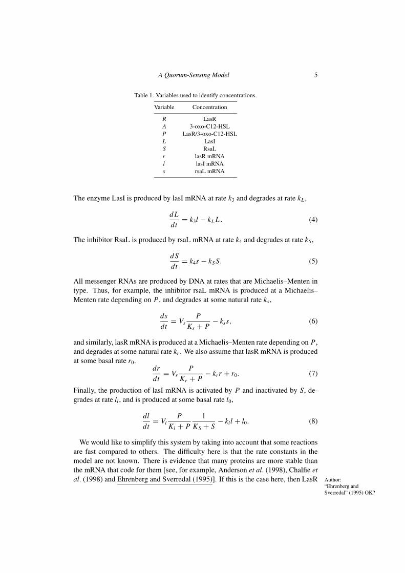
Table 1. Variables used to identify concentrations.

Variable Concentration

R LasRA 3-oxo-C12-HSLP LasR/3-oxo-C12-HSLL LasIS RsaLr lasR mRNAl lasI mRNAs rsaL mRNA

The enzyme LasI is produced by lasI mRNA at rate k3 and degrades at rate kL ,

d L

dt= k3l − kL L . (4)

The inhibitor RsaL is produced by rsaL mRNA at rate k4 and degrades at rate kS ,

d S

dt= k4s − kS S. (5)

All messenger RNAs are produced by DNA at rates that are Michaelis–Menten intype. Thus, for example, the inhibitor rsaL mRNA is produced at a Michaelis–Menten rate depending on P , and degrades at some natural rate ks ,

ds

dt= Vs

P

Ks + P− kss, (6)

and similarly, lasR mRNA is produced at a Michaelis–Menten rate depending on P ,and degrades at some natural rate kr . We also assume that lasR mRNA is producedat some basal rate r0.

dr

dt= Vr

P

Kr + P− krr + r0. (7)

Finally, the production of lasI mRNA is activated by P and inactivated by S, de-grades at rate ll , and is produced at some basal rate l0,

dl

dt= Vl

P

Kl + P

1

KS + S− kll + l0. (8)

We would like to simplify this system by taking into account that some reactionsare fast compared to others. The difficulty here is that the rate constants in themodel are not known. There is evidence that many proteins are more stable thanthe mRNA that code for them [see, for example, Anderson et al. (1998), Chalfie etal. (1998) and Ehrenberg and Sverredal (1995)]. If this is the case here, then LasR Author:

“Ehrenberg andSverredal” (1995) OK?


mRNA and lasI mRNA are much shorter lived than LasR and LasL, respectively,so that kr and kl are much larger than kL and kR . With this assumption, we take land r to be in quasi-steady state, so that

kll = VlP

Kl + P

1

KS + S+ l0, krr = Vr

P

Kr + P+ r0. (9)

The variable L can be understood as a first-order linear filter, so that L tracks lwith some delay. The simplest approximation to this behavior is to ignore the delayand take

k3l = kL L . (10)

The quantity S inhibits the production of l, but it seems not to have much effecton quorum-sensing behavior. We ignore this variable by eliminating it from theproduction term in equation (8).

With these simplifications, the governing system of equations becomes

d P

dt= kR A R A − kP P, (11)

d R

dt=−kR A R A + kP P − kR R + VR

P

K R + P+ R0, (12)

d A

dt=−kR A R A + kP P + VA

P

KL + P+ A0 − kA A, (13)

(with redefined parameters, of course). Finally, since the production of A and RAuthor:Equation number (14)avoided afterequation (13) OK? (pleasecheck hard copy)

involves transcription of mRNA, it is probably slow compared to the binding andunbinding of R and A to form complex P . Thus, we assume that P is in quasi-steady state so that

kP P = kR A R A (14)

and the governing equations become

d R

dt=−kR R + VR

P

K R + P+ R0, (15)

d A

dt= VA

P

KL + P+ A0 − kA A, (16)

P = kR A

kPR A. (17)

Next, we need to determine how the density of organisms controls the activityof this network. We assume that autoinducer A diffuses across the cell membrane,and that the local density (volume fraction) of cells is ρ. Then by assumption, thelocal volume fraction of extracellular space is 1− ρ.


The extracellular autoinducer is assumed to diffuse freely across the cell mem-brane, with conductance δ, and naturally degrades at rate kE . If we suppose thatthe density of cells is uniform and the extracellular space is well mixed, then theconcentration of autoinducer in the extracellular space, denoted E , is governed bythe equation

(1− ρ)

(d E

dt+ kE E

)= δ(A − E). (18)

Here the factor 1− ρ must be included to scale for the difference between concen-tration in the extracellular space and concentration viewed as amount per unit totalvolume. Similarly, the governing equation for intracellular autoinducer A must bemodified to account for diffusion across the cell membrane, yielding

ρ

(d A

dt− VA

P

KL + P− A0 + kA A

)= −δ(A − E). (19)

There is some evidence that the transport of the autoinducer may involve bothpassive diffusion and a cotransport mechanism (Pearson et al., 1999). For thismodel we assume that diffusion alone acts to transport the autoinducer [as is ap-parently correct for the rhl system (Pearson et al., 1999)]. The inclusion here of anadditional cotransport mechanism is possible but seems not to be a crucial ingredi-ent.

It is now fairly easy to see that this system of equations exhibits quorum sensing.One way to see this is to take E to be in quasi-steady state. This is probably nota good assumption since A and E are the same chemical and so probably degradeat about the same rates inside and outside the cell. However, this assumption al-lows us to study this system in the phase plane. The behavior is not changed ifa three-variable system is used, but the analysis of the three-variable systems issubstantially more complicated with little increase in insight.

The resulting system is (with redefined parameters)

d R

dt= VR

P

K R + P− kR R + R0, (20)

d A

dt= VA

P

K A + P+ A0 − d(ρ)A, (21)

where P = kR A R AkP

and d(ρ) = kA + δρ

( kE (1−ρ)

δ+kE (1−ρ)

).

Quorum sensing works because of the ρ dependence of d(ρ). In particular, whenρ is small, d(ρ), the decay rate for A, is large, while when ρ is close to one, d(ρ)

is small. This has the feature of modifying the A nullcline in an important way.The nullclines for the system (20), (21) are shown in Fig. 2. Here it is readily seenthat for small values of ρ and for large values of ρ there is a unique steady-statesolution in the positive R–A quadrant. For small values of ρ the steady-state values


4

3

2

1

0

A

0 1 2 3 4

R

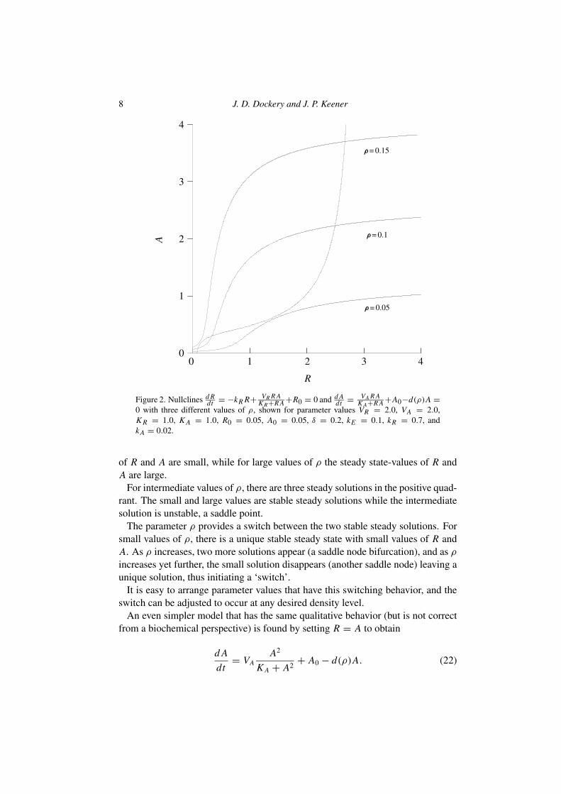
Figure 2. Nullclines d Rdt = −kR R+ VR R A

K R+R A+R0 = 0 and d Adt = VA R A

K A+R A+A0−d(ρ)A =0 with three different values of ρ, shown for parameter values VR = 2.0, VA = 2.0,K R = 1.0, K A = 1.0, R0 = 0.05, A0 = 0.05, δ = 0.2, kE = 0.1, kR = 0.7, andkA = 0.02.

of R and A are small, while for large values of ρ the steady state-values of R andA are large.

For intermediate values of ρ, there are three steady solutions in the positive quad-rant. The small and large values are stable steady solutions while the intermediatesolution is unstable, a saddle point.

The parameter ρ provides a switch between the two stable steady solutions. Forsmall values of ρ, there is a unique stable steady state with small values of R andA. As ρ increases, two more solutions appear (a saddle node bifurcation), and as ρ

increases yet further, the small solution disappears (another saddle node) leaving aunique solution, thus initiating a ‘switch’.

It is easy to arrange parameter values that have this switching behavior, and theswitch can be adjusted to occur at any desired density level.

An even simpler model that has the same qualitative behavior (but is not correctfrom a biochemical perspective) is found by setting R = A to obtain

d A

dt= VA

A2

K A + A2+ A0 − d(ρ)A. (22)


0.2

0.1

0.0

− 0.1

− 0.2

dA/d

t

A0 1 2 3

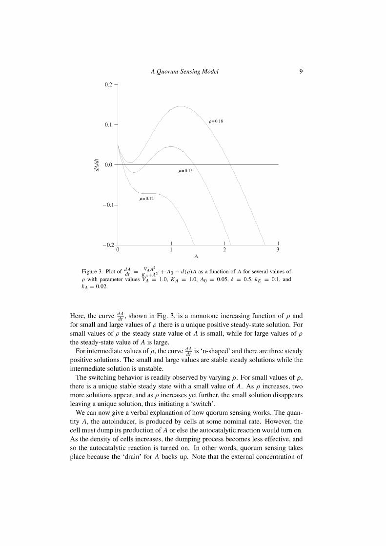
Figure 3. Plot of d Adt = VA A2

K A+A2 + A0 − d(ρ)A as a function of A for several values ofρ with parameter values VA = 1.0, K A = 1.0, A0 = 0.05, δ = 0.5, kE = 0.1, andkA = 0.02.

Here, the curve d Adt , shown in Fig. 3, is a monotone increasing function of ρ and

for small and large values of ρ there is a unique positive steady-state solution. Forsmall values of ρ the steady-state value of A is small, while for large values of ρ

the steady-state value of A is large.For intermediate values of ρ, the curve d A

dt is ‘n-shaped’ and there are three steadypositive solutions. The small and large values are stable steady solutions while theintermediate solution is unstable.

The switching behavior is readily observed by varying ρ. For small values of ρ,there is a unique stable steady state with a small value of A. As ρ increases, twomore solutions appear, and as ρ increases yet further, the small solution disappearsleaving a unique solution, thus initiating a ‘switch’.

We can now give a verbal explanation of how quorum sensing works. The quan-tity A, the autoinducer, is produced by cells at some nominal rate. However, thecell must dump its production of A or else the autocatalytic reaction would turn on.As the density of cells increases, the dumping process becomes less effective, andso the autocatalytic reaction is turned on. In other words, quorum sensing takesplace because the ‘drain’ for A backs up. Note that the external concentration of


A is always smaller than the internal concentration of A. Thus, A is not actually asignaling chemical, and there is no necessity for surface receptors for A, and thereis no need to develop high concentrations of autoinducer in the extracellular space.

3. A PDE MODEL

While the above model shows the desired behavior in a homogeneous environ-ment, such as a chemostat, a more realistic model would take into account thepossibility of inhomogeneous distributions of the autoinducer in the extracellularspace, while the cells themselves remain relatively motionless.

We suppose there is a uniform layer of cells of thickness L and fixed volumefraction ρ which are attached to a substratum in an aqueous bath. As above, thecells produce the autoinducer with concentration A which has extracellular con-centration E ,

d A

dt= F(A)+ δ

ρ(E − A), (23)

∂ E

∂t= ∂2 E

∂x2+ δ

1− ρ(A − E)− kE E . (24)

The factor ρ in equation (23) and the factor 1− ρ in (24) are necessary to accountfor the differences in volume fraction between intracellular and extracellular space.We assume that the cells occupy the one-dimensional region 0 < x < L . At theboundary of the cellular domain, x = L , we assume that there is mass transfer intothe bulk fluid. We model this simply by assuming the Robin boundary condition

Ex(L , t)+ αE(L , t) = 0 (25)

where α is a positive parameter. At the substratum we impose the Neumann bound-ary condition

Ex(0, t) = 0. (26)

The goal of this section is to find the steady-state solutions of this pde, i.e.,

Exx + δ

1− ρ(A − E)− kE E = 0, with F(A)+ δ

ρ(E − A) = 0 (27)

on 0 < x < L with Ex(0) = 0 and Ex(L)+ αE(L) = 0.The analysis of this equation is accomplished in the phase plane. First, we must

determine the nature of the solutions of the equation

F(A)+ δ

ρ(E − A) = 0. (28)


5

4

3

2

1

0

E

543210A

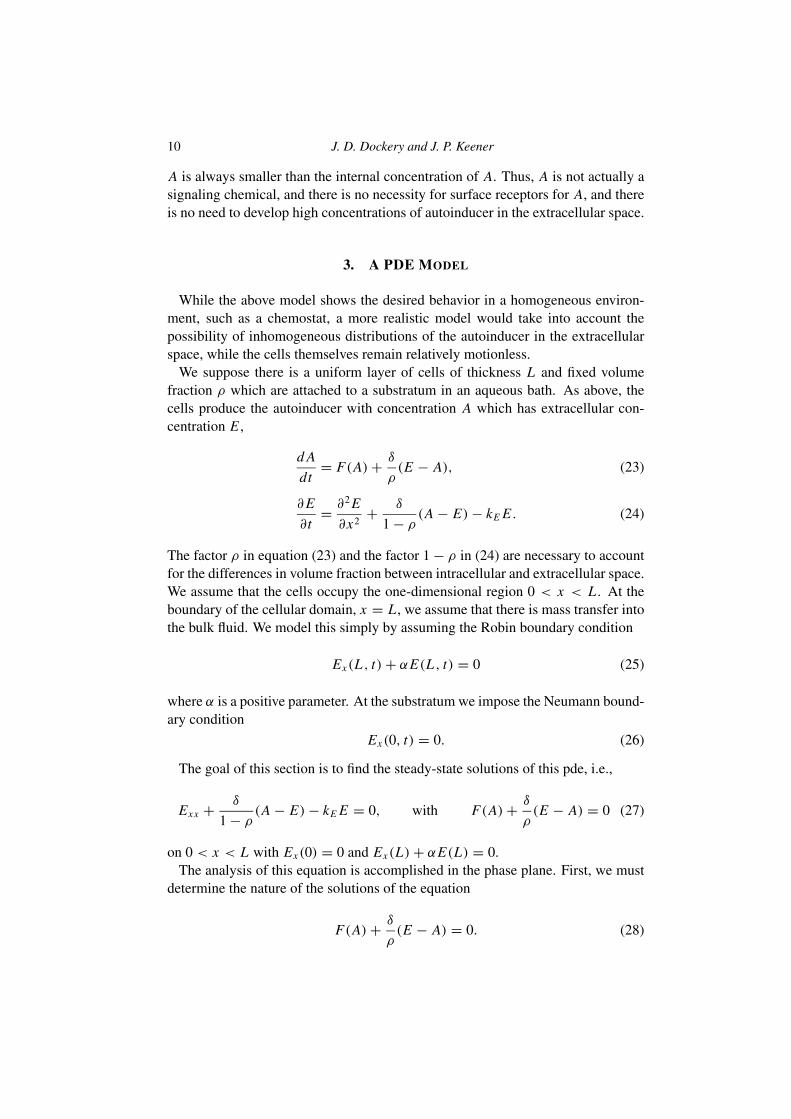
Figure 4. Plot of the function E(A) = A − ρδ F(A) for K A = 1.0, VA = 1.0, A0 = 0.05,

δ = 0.1, ρ = 0.3, and kA = 0.2.

0.20

0.15

0.10

0.05

0.00

g(E

)

2.01.51.00.50.0− 0.5

E

g+(E)

g0(E)

g−(E)

EmxEmn E0

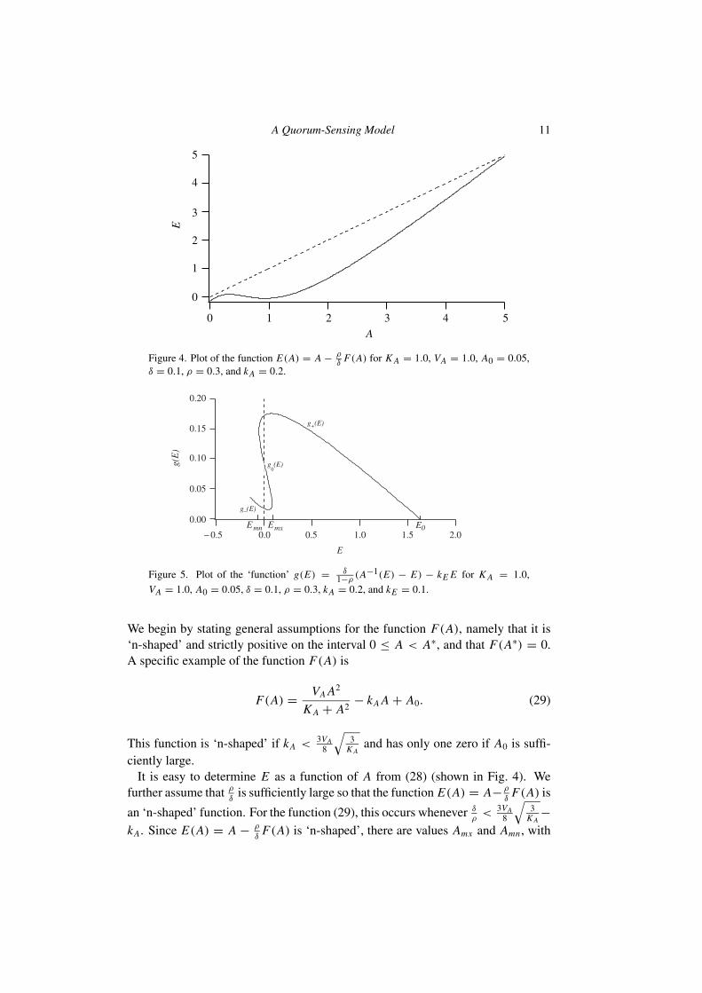
Figure 5. Plot of the ‘function’ g(E) = δ1−ρ

(A−1(E) − E) − kE E for K A = 1.0,

VA = 1.0, A0 = 0.05, δ = 0.1, ρ = 0.3, kA = 0.2, and kE = 0.1.

We begin by stating general assumptions for the function F(A), namely that it is‘n-shaped’ and strictly positive on the interval 0 ≤ A < A∗, and that F(A∗) = 0.A specific example of the function F(A) is

F(A) = VA A2

K A + A2− kA A + A0. (29)

This function is ‘n-shaped’ if kA < 3VA8

√3

K Aand has only one zero if A0 is suffi-

ciently large.It is easy to determine E as a function of A from (28) (shown in Fig. 4). We

further assume that ρ

δis sufficiently large so that the function E(A) = A− ρ

δF(A) is

an ‘n-shaped’ function. For the function (29), this occurs whenever δρ

< 3VA8

√3

K A−

kA. Since E(A) = A − ρ

δF(A) is ‘n-shaped’, there are values Amx and Amn , with


0.50

0.25

0.00

− 0.25

− 0.500.0 0.5 1.0 1.5

E

dE/d

x

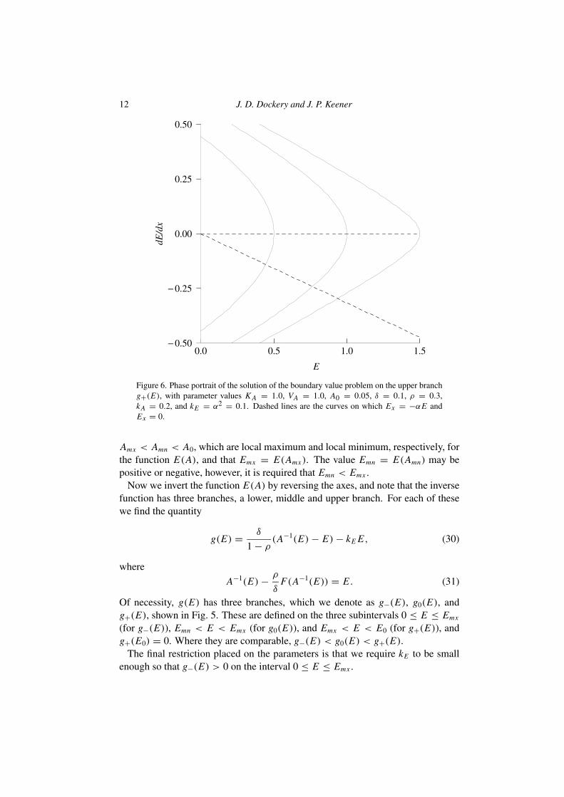
Figure 6. Phase portrait of the solution of the boundary value problem on the upper branchg+(E), with parameter values K A = 1.0, VA = 1.0, A0 = 0.05, δ = 0.1, ρ = 0.3,kA = 0.2, and kE = α2 = 0.1. Dashed lines are the curves on which Ex = −αE andEx = 0.

Amx < Amn < A0, which are local maximum and local minimum, respectively, forthe function E(A), and that Emx = E(Amx). The value Emn = E(Amn) may bepositive or negative, however, it is required that Emn < Emx .

Now we invert the function E(A) by reversing the axes, and note that the inversefunction has three branches, a lower, middle and upper branch. For each of thesewe find the quantity

g(E) = δ

1− ρ(A−1(E)− E)− kE E, (30)

where

A−1(E)− ρ

δF(A−1(E)) = E . (31)

Of necessity, g(E) has three branches, which we denote as g−(E), g0(E), andg+(E), shown in Fig. 5. These are defined on the three subintervals 0 ≤ E ≤ Emx

(for g−(E)), Emn < E < Emx (for g0(E)), and Emx < E < E0 (for g+(E)), andg+(E0) = 0. Where they are comparable, g−(E) < g0(E) < g+(E).

The final restriction placed on the parameters is that we require kE to be smallenough so that g−(E) > 0 on the interval 0 ≤ E ≤ Emx .


1.6

1.2

0.8

0.4

0.00 2 4 6 8 10

L

E(0

)

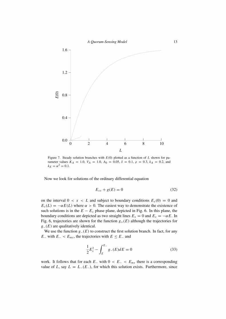
Figure 7. Steady solution branches with E(0) plotted as a function of L shown for pa-rameter values K A = 1.0, VA = 1.0, A0 = 0.05, δ = 0.1, ρ = 0.3, kA = 0.2, andkE = α2 = 0.1.

Now we look for solutions of the ordinary differential equation

Exx + g(E) = 0 (32)

on the interval 0 < x < L and subject to boundary conditions Ex(0) = 0 andEx(L) = −αE(L) where α > 0. The easiest way to demonstrate the existence ofsuch solutions is in the E − Ex phase plane, depicted in Fig. 6. In this plane, theboundary conditions are depicted as two straight lines Ex = 0 and Ex = −αE . InFig. 6, trajectories are shown for the function g+(E) although the trajectories forg−(E) are qualitatively identical.

We use the function g−(E) to construct the first solution branch. In fact, for anyE− with E− < Emx , the trajectories with E ≤ E− and

1

2E2

x −∫ E−

Eg−(E)d E = 0 (33)

work. It follows that for each E− with 0 < E− < Emx there is a correspondingvalue of L , say L = L−(E−), for which this solution exists. Furthermore, since


0.6

0.5

0.4

0.3

0.2

0.1

0.00.0 0.2 0.4 0.6 0.8 1.0

x

E

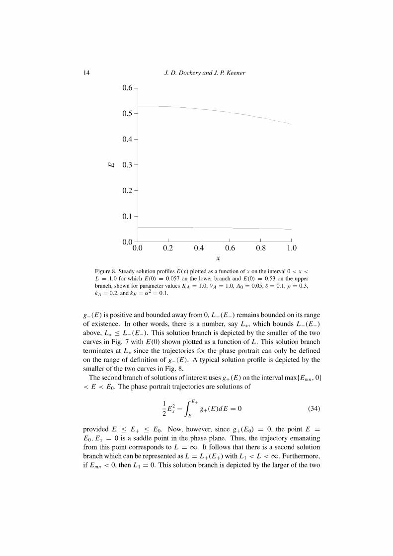
Figure 8. Steady solution profiles E(x) plotted as a function of x on the interval 0 < x <

L = 1.0 for which E(0) = 0.057 on the lower branch and E(0) = 0.53 on the upperbranch, shown for parameter values K A = 1.0, VA = 1.0, A0 = 0.05, δ = 0.1, ρ = 0.3,kA = 0.2, and kE = α2 = 0.1.

g−(E) is positive and bounded away from 0, L−(E−) remains bounded on its rangeof existence. In other words, there is a number, say L∗, which bounds L−(E−)above, L∗ ≤ L−(E−). This solution branch is depicted by the smaller of the twocurves in Fig. 7 with E(0) shown plotted as a function of L . This solution branchterminates at L∗ since the trajectories for the phase portrait can only be definedon the range of definition of g−(E). A typical solution profile is depicted by thesmaller of the two curves in Fig. 8.

The second branch of solutions of interest uses g+(E) on the interval max{Emn, 0}< E < E0. The phase portrait trajectories are solutions of

1

2E2

x −∫ E+

Eg+(E)d E = 0 (34)

provided E ≤ E+ ≤ E0. Now, however, since g+(E0) = 0, the point E =E0, Ex = 0 is a saddle point in the phase plane. Thus, the trajectory emanatingfrom this point corresponds to L = ∞. It follows that there is a second solutionbranch which can be represented as L = L+(E+) with L1 < L <∞. Furthermore,if Emn < 0, then L1 = 0. This solution branch is depicted by the larger of the two


0.4

0.3

0.2

0.1

0.0-0.5 0.0 0.5 1.0 1.5 2.0

E

g(E

)

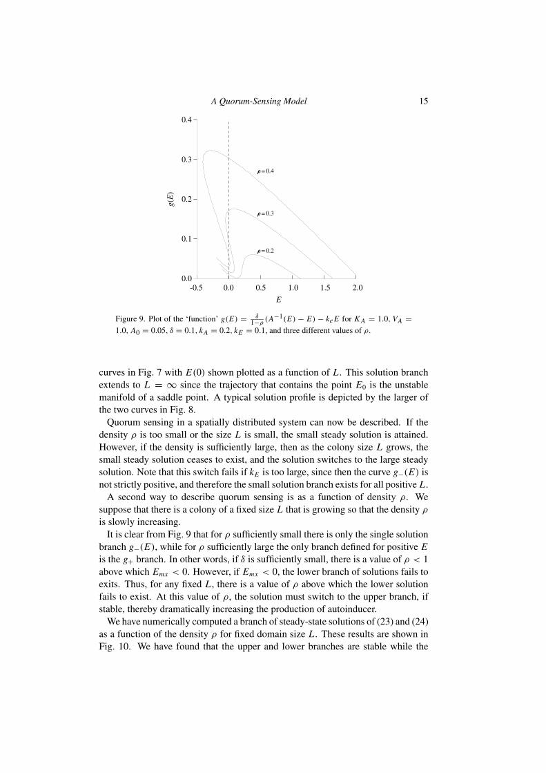
Figure 9. Plot of the ‘function’ g(E) = δ1−ρ

(A−1(E) − E) − ke E for K A = 1.0, VA =1.0, A0 = 0.05, δ = 0.1, kA = 0.2, kE = 0.1, and three different values of ρ.

curves in Fig. 7 with E(0) shown plotted as a function of L . This solution branchextends to L = ∞ since the trajectory that contains the point E0 is the unstablemanifold of a saddle point. A typical solution profile is depicted by the larger ofthe two curves in Fig. 8.

Quorum sensing in a spatially distributed system can now be described. If thedensity ρ is too small or the size L is small, the small steady solution is attained.However, if the density is sufficiently large, then as the colony size L grows, thesmall steady solution ceases to exist, and the solution switches to the large steadysolution. Note that this switch fails if kE is too large, since then the curve g−(E) isnot strictly positive, and therefore the small solution branch exists for all positive L .

A second way to describe quorum sensing is as a function of density ρ. Wesuppose that there is a colony of a fixed size L that is growing so that the density ρ

is slowly increasing.It is clear from Fig. 9 that for ρ sufficiently small there is only the single solution

branch g−(E), while for ρ sufficiently large the only branch defined for positive Eis the g+ branch. In other words, if δ is sufficiently small, there is a value of ρ < 1above which Emx < 0. However, if Emx < 0, the lower branch of solutions fails toexits. Thus, for any fixed L , there is a value of ρ above which the lower solutionfails to exist. At this value of ρ, the solution must switch to the upper branch, ifstable, thereby dramatically increasing the production of autoinducer.

We have numerically computed a branch of steady-state solutions of (23) and (24)as a function of the density ρ for fixed domain size L . These results are shown inFig. 10. We have found that the upper and lower branches are stable while the


0 0.1 0.2 0.3 0.4 0.5 0.6 0.7 0.8 0.9 10

1

2

3

4

5

6

A(0

)

Figure 10. Plot of the bifurcation diagram for the steady states of (23) as a function of thecell density ρ with L fixed at L = 2. The parameter values are K A = 1.0, VA = 1.0, A0 =0.05, δ = 0.1, kA = 0.2, kE = 0.1, ρ = 0.3, α = 1.0, and L = 2.0.

middle branch is unstable. As the cell density increases, the production of the au-toinducer increases slowly until a critical value of the density is reached. At thispoint there is a large increase in autoinducer production. Once on the upper branch,the population maintains a high rate of autoinducer production even if the cell den-sity decreases. However, if the cell density falls below the value at the knee on theupper branch, production falls back to a nominal rate.

It has been shown (Davies et al., 1998) that autoinducers can increase polymerproduction. With increased polymer the cell density would decrease. Thus we seethat hysteresis assures that the switch to high autoinducer production is not easilyreversed by a decrease in cell density due to an increase in polymer production.It is also easy to speculate that once the cell density becomes low enough that theautoinducer is reset to basal levels, the genes responsible for polymer productionare turned off. If there is too much polymer, the diffusion of vital nutrients to thepopulation could be hindered.

In summary, quorum sensing can be accomplished by increasing the density of acolony of fixed size, or by increasing the size of a colony of large enough density.

In the next section, stability results are discussed.

4. STABILITY RESULTS

The stability of the steady state can be determined by numerical simulations ofthe system or by linearization (Weinberger, 1983).

The following proposition implies that the large and small amplitude steady-statesolutions to our system are stable provided that on the range of the steady solution


0 0.2 0.4 0.6 0.8 10.2

0.4

0.6

0.8

1

1.2

1.4

1.6

1.8

2L = 2

AE

0 0.2 0.4 0.6 0.8 10.02

0.04

0.06

0.08

0.1

0.12

0.14

0.16

0.18

0.2

0.22L = 2

AE

x x

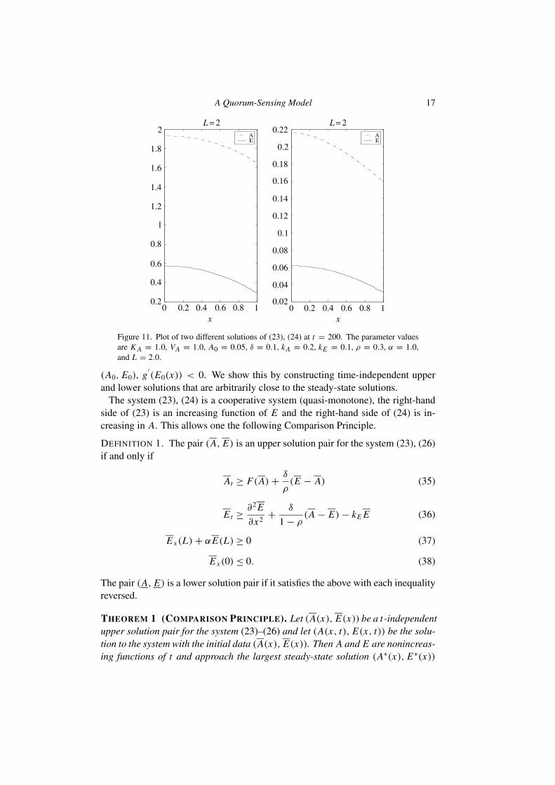
Figure 11. Plot of two different solutions of (23), (24) at t = 200. The parameter valuesare K A = 1.0, VA = 1.0, A0 = 0.05, δ = 0.1, kA = 0.2, kE = 0.1, ρ = 0.3, α = 1.0,and L = 2.0.

(A0, E0), g′(E0(x)) < 0. We show this by constructing time-independent upper

and lower solutions that are arbitrarily close to the steady-state solutions.The system (23), (24) is a cooperative system (quasi-monotone), the right-hand

side of (23) is an increasing function of E and the right-hand side of (24) is in-creasing in A. This allows one the following Comparison Principle.

DEFINITION 1. The pair (A, E) is an upper solution pair for the system (23), (26)if and only if

At ≥ F(A)+ δ

ρ(E − A) (35)

Et ≥ ∂2 E

∂x2+ δ

1− ρ(A − E)− kE E (36)

E x(L)+ αE(L) ≥ 0 (37)

E x(0) ≤ 0. (38)

The pair (A, E) is a lower solution pair if it satisfies the above with each inequalityreversed.

THEOREM 1 (COMPARISON PRINCIPLE). Let (A(x), E(x)) be a t-independentupper solution pair for the system (23)–(26) and let (A(x, t), E(x, t)) be the solu-tion to the system with the initial data (A(x), E(x)). Then A and E are nonincreas-ing functions of t and approach the largest steady-state solution (A∗(x), E∗(x))


L E(0)

3

2.5

2

1.5

1

0.5

00 20 40 60 80 100 120 140 160 180 200

t

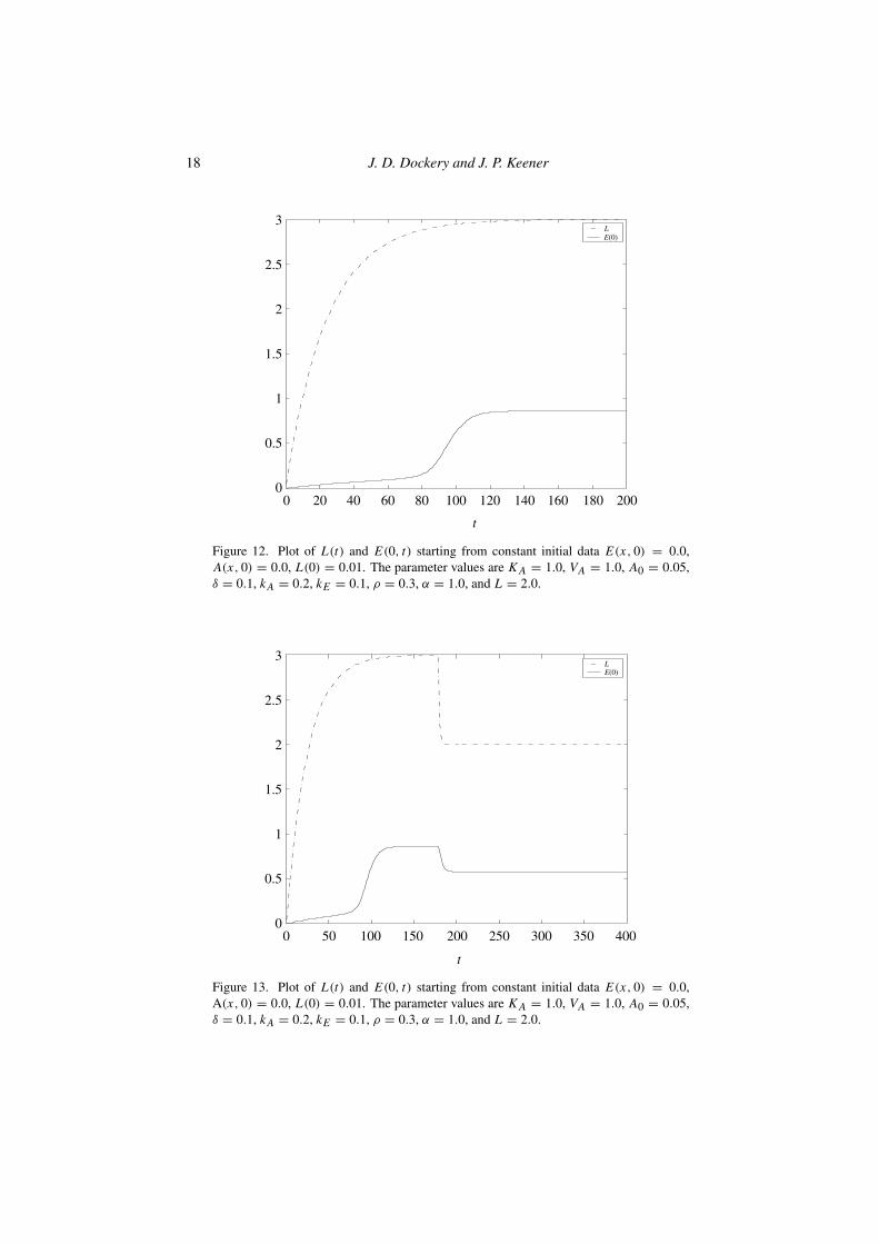
Figure 12. Plot of L(t) and E(0, t) starting from constant initial data E(x, 0) = 0.0,A(x, 0) = 0.0, L(0) = 0.01. The parameter values are K A = 1.0, VA = 1.0, A0 = 0.05,δ = 0.1, kA = 0.2, kE = 0.1, ρ = 0.3, α = 1.0, and L = 2.0.

L E(0)

3

2.5

2

1.5

1

0.5

00 50 100 150 200 250 300 350 400

t

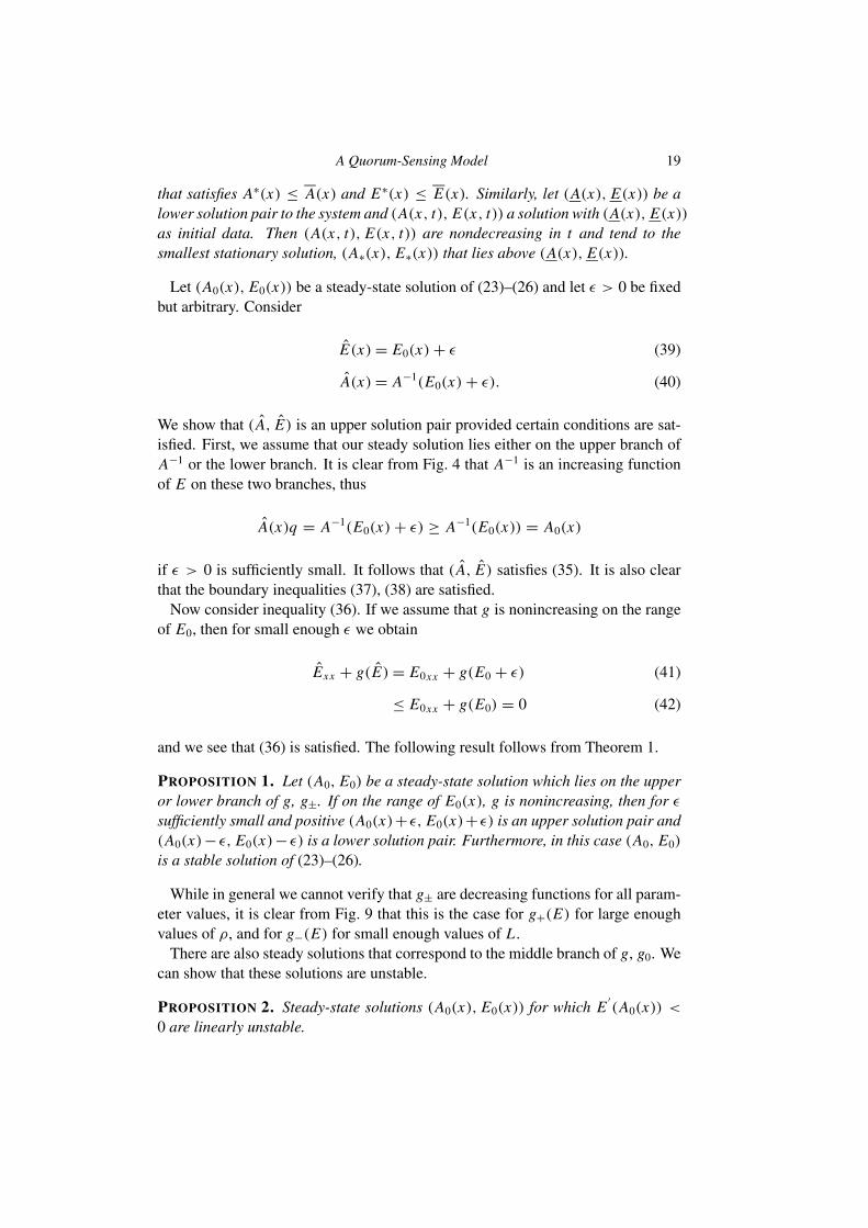
Figure 13. Plot of L(t) and E(0, t) starting from constant initial data E(x, 0) = 0.0,A(x, 0) = 0.0, L(0) = 0.01. The parameter values are K A = 1.0, VA = 1.0, A0 = 0.05,δ = 0.1, kA = 0.2, kE = 0.1, ρ = 0.3, α = 1.0, and L = 2.0.


that satisfies A∗(x) ≤ A(x) and E∗(x) ≤ E(x). Similarly, let (A(x), E(x)) be alower solution pair to the system and (A(x, t), E(x, t)) a solution with (A(x), E(x))

as initial data. Then (A(x, t), E(x, t)) are nondecreasing in t and tend to thesmallest stationary solution, (A∗(x), E∗(x)) that lies above (A(x), E(x)).

Let (A0(x), E0(x)) be a steady-state solution of (23)–(26) and let ε > 0 be fixedbut arbitrary. Consider

E(x)= E0(x)+ ε (39)

A(x)= A−1(E0(x)+ ε). (40)

We show that ( A, E) is an upper solution pair provided certain conditions are sat-isfied. First, we assume that our steady solution lies either on the upper branch ofA−1 or the lower branch. It is clear from Fig. 4 that A−1 is an increasing functionof E on these two branches, thus

A(x)q = A−1(E0(x)+ ε) ≥ A−1(E0(x)) = A0(x)

if ε > 0 is sufficiently small. It follows that ( A, E) satisfies (35). It is also clearthat the boundary inequalities (37), (38) are satisfied.

Now consider inequality (36). If we assume that g is nonincreasing on the rangeof E0, then for small enough ε we obtain

Exx + g(E)= E0xx + g(E0 + ε) (41)

≤ E0xx + g(E0) = 0 (42)

and we see that (36) is satisfied. The following result follows from Theorem 1.

PROPOSITION 1. Let (A0, E0) be a steady-state solution which lies on the upperor lower branch of g, g±. If on the range of E0(x), g is nonincreasing, then for ε

sufficiently small and positive (A0(x)+ ε, E0(x)+ ε) is an upper solution pair and(A0(x)− ε, E0(x)− ε) is a lower solution pair. Furthermore, in this case (A0, E0)

is a stable solution of (23)–(26).

While in general we cannot verify that g± are decreasing functions for all param-eter values, it is clear from Fig. 9 that this is the case for g+(E) for large enoughvalues of ρ, and for g−(E) for small enough values of L .

There are also steady solutions that correspond to the middle branch of g, g0. Wecan show that these solutions are unstable.

PROPOSITION 2. Steady-state solutions (A0(x), E0(x)) for which E′(A0(x)) <

0 are linearly unstable.


To prove this, consider the linearization of (23), (24) about a steady solution(A0, E0)

at = F′ [A0(x)]a + δ

ρ(e − a), (43)

et = exx + δ

1− ρ(a − e)− kE e. (44)

Let α(x) = F′ [A0(x)] − δ

ρ, and note that α(x) = −ρ

δE′ [A0(x)], which is pos-

itive on the middle branch. Suppose that (a, e) is a solution of (43), (44) with(a(x, 0), e(x, 0)) = (a0(x), e0(x)) and such that e(x, t) remains bounded for allt ≥ 0, say |e(x, t)| ≤ M . Then from (43) we see that

at ≥ α(x)a − Mδ

ρ

which implies that

a(x, t) ≥ exp(α(x)t)a0(0)+ Mδ

ρα(x)(1− exp(α(x)t))

so that a(x, t) cannot remain bounded for all t > 0 if we start with positive initialdata, which implies instability. If e(x, t) is unbounded for t > 0 starting fromarbitrarily small initial data, then clearly the steady solution is linearly unstable.

5. NUMERICAL SIMULATIONS

In this section we report on numerical simulations which illustrate the stabilityresults of the previous section. We also indicate how these results may be applica-ble to biofilms.

We take α = 1 and scale the x interval to have unit length. In Fig. 11 aredisplayed the two stable steady states that exist when L = 2. One is an orderof magnitude larger than the other. The small solution was generated from theconstant initial data A(x, 0) = 0.0 and E(x, 0) = 0. The larger solution wasalso generated from constant initial data, A(x, 0) = 1.0 and E(x, 0) = 1.0. Bothsolutions are shown at time t = 200. At this time the time derivatives of both Aand E are less than 10−10 so we take these to be steady states.

One can model a growing population by adding dynamics for the domain lengthL . Here we set

d L

dt= κ(L f − L) (45)

where κ = 0.04 and L f = 3.


The time series of a solution of (23), (24) and (45) with constant initial data isshown in Fig. 12. Here we display the length of the interval L and the value ofthe extracellular autoinducer at x = 0, E(0, t) as functions of time. From othernumerical calculations we know that the small amplitude solution does not exist atL = 2.2. We see that after a lag the solution of the evolution equation approachesthe large amplitude steady solution that exists at L = 3.

To demonstrate the hysteresis indicated in Fig. 7, we use the same dynamics forL as above in a second run until t = 180 whereupon we set L = 2. This could bethought of as a major detachment event whereby the biofilm thickness is suddenlyreset to two thirds of its asymptotic thickness. The time series of such a solutionis shown in Fig. 13. We see that upon reset, the autoinducer concentration remainshigh. The hysteresis assures that the switch to high autoinducer production is noteasily reversed. This is very important for a biofilm since these populations areoften subjected to major detachment and sluffing events whereby there are largeand sudden decreases in population size.

6. DISCUSSION

We have presented a simple model of quorum sensing using autoinduction that isbased on the known biochemistry of P. aeruginosa. Using this model we demon-strate that quorum sensing works because the rate of elimination of autoinducerdepends on the colony size and density. Thus, the autoinducer production switchesto its high state when the elimination of autoinducer from the extracellular space isdecreased.

This biochemical switch is hysteretic so that autoinducer production switches onat different (higher) levels than it switches off. This hysteresis is possibly importantin the regulation of the production of exopolysaccharide, which tends to decreasebacterial density. The hysteresis predicted by this model investigation has not beenverified experimentally.

ACKNOWLEDGEMENTS

JDD was supported in part by NSF grant DMS-9805701. JPK was supported inpart by NSF grant DMS-99700876.

REFERENCES

Anderson, J. B., C. Sternberg, L. K. Poulsen, M. Givskov and S. Molin (1998). New Editor:position of reference VanDelden andIglewski(1998) OK?(Alphabetical order)

unstable variants of green fluorescent protein for studies of transient gene expression inbacteria. Appl. Environ. Microbiol. 64, 2240–2246.

Chalfie, M., Y. Tu, G. Euskirchen, W. W. Ward and D. C. Prasher (1994). Green fluores-cent protein as a marker for gene expression. Science 263, 802–805.


Characklis, W. G. and K. C. Marshall (1990). Biofilms, New York: John Wiley & Sons,Inc.

Davies, D. G., M. R. Parsek, J. P. Pearson, B. H. Iglewski, J. W. Costerton and E. P.Author:Please supply more detailsof reference Davies et al.(1998)

Greenberg (1998). The involvement of cell-to-cell signals in the development of bacte-rial biofilm. Science.

Van Delden, C. and B. H. Iglewski (1998). Cell-to-cell signaling and Pseudomonas aerug-Author:Please supply more

details of reference VanDelden et al. (1998);Editor:Issue number OK?

inosa infections. Emerging Infect. Dis. 4(4).Ehrenberg, M. and A. Sverredal (1995). A model for copy number control of the plasmid

R1. J. Mol. Biol. 246, 472–485.Fuqua, C., S. C. Winans and E. P. Greenberg (1996). Census and concensus in bacterial

ecosystems: The luxR-luxI family of quorum-sensing transcriptional regulators. Annu.Rev. Microbiol. 50, 727–751.

Govan, J. R. and V. Deretic (1996). Microbial pathogenesis in cystic fibrosis: mucoidAuthor:Please supply more detailsof reference Govan andDeretic (1996)

pseudomonas aeruginosa and Burkolderia cepacia. Microbiol. Rev.James, S., P. Nilsson, G. James, S. Kjelleberg and T. Fagerstrom (2000). Luminescence

control in the marine bacterium Vibrio fischeri: An analysis of the dynamics of luxregulation. J. Mol. Biol. 296, 1127–1137.

Pearson, J. P., C. Van Delden and B. H. Iglewski (1999). Active efflux and diffusionare involved in transport of Pseudomonas aeruginosa cell-to-cell signals. J. Bacteriol.181(4), 1203–1210.Editor:

Issue number OK? Ward, J. P., J. R. King and A. J. Koerber (2000). Mathematical modelling of quorum sens-ing in bacteria. Preprint.

Weinberger, H. F. (1983). A simple system with a continuum of stable inhomoge-neous steady states, in Nonlinear Partial Differential Equations in Applied Science(Tokyo, 1982), Amsterdam: North-Holland, pp. 345–359.

Received 16 January 2000 and accepted 3 September 2000

A Mathematical Model for Quorum Sensing in …keener/pubs/papers/bulm0205.pdf · A Mathematical...

Documents

Transcript of A Mathematical Model for Quorum Sensing in …keener/pubs/papers/bulm0205.pdf · A Mathematical...