Research Division Federal Reserve Bank of St. Louis Working Paper Series

A Macroeconomic Analysis of Obesity

Pere Gomis-Porqueras and

Adrian Peralta-Alva

Working Paper 2008-017A http://research.stlouisfed.org/wp/2008/2008-017.pdf

June 2008

FEDERAL RESERVE BANK OF ST. LOUIS Research Division

P.O. Box 442 St. Louis, MO 63166

______________________________________________________________________________________

The views expressed are those of the individual authors and do not necessarily reflect official positions of the Federal Reserve Bank of St. Louis, the Federal Reserve System, or the Board of Governors.

Federal Reserve Bank of St. Louis Working Papers are preliminary materials circulated to stimulate discussion and critical comment. References in publications to Federal Reserve Bank of St. Louis Working Papers (other than an acknowledgment that the writer has had access to unpublished material) should be cleared with the author or authors.

A Macroeconomic Analysis of Obesity∗

Pere Gomis-Porqueras

Department of Economics

University of Miami

Adrian Peralta-Alva †

Research Division

Federal Reserve Bank of Saint Louis

Abstract

This paper tries to understand the underlying causes of the rapid increase in obesity rates over recentdecades. In particular, we propose a dynamic general equilibrium model to derive the quantitativeimplications of a decline in the relative (monetary and time) cost of food prepared away from homeon the caloric intake of the average American adult over the last forty years. Two channels thatlower this relative cost are considered. First, productivity improvements in the production of foodprepared away from home. We find that this channel is qualitatively consistent with expendituretrends in food items, but falls short of accounting for the magnitude of the observed changes. Wethen consider actual declines in income taxes and in the gender wage gap, which increase the costof preparing food at home from scratch. Our model accounts for three quarters of the observedchanges in calorie consumption, and is consistent with trends in aggregate food expenditures, timeuse, and key macroeconomic variables. Our results indicate that changes in the relative cost of foodprepared away from home play an important role in our understanding of the increased weight ofthe American population during the last 40 years.

JEL Classification: E1, E2.Keywords: Taxes, Gender Wage Gap, Female Labor Participation, Obesity.

∗We would like to thank Olivia Thomas for her insightful comments on obesity issues, Nuray Akin, Frank Heiland,Ayse Imrohoroglu, Dave Kelly, Ellen McGrattan, Oscar Mitnik, Manuel Santos, Jesse Shapiro, Michele Tertilt and theseminar participants of the 2006 Annual Meeting of the SED, the University of Miami, the Federal Reserve Bank ofAtlanta, the University of Waterloo, Western Ontario and the Midwest Macro Meetings for their helpful comments.Adrian Peralta acknowledges the support of the James W. McLamore Summer Awards in Business and Social Sciencesof the University of Miami.†The views expressed are those of the individual authors and do not necessarily reflect official positions of the Federal

Reserve Bank of St. Louis, the Federal Reserve System, or the Board of Governors.

1

1 Introduction

Many countries have experienced a startling increase in obesity rates over the last 10-20 years. Forthe first time, the number of overweight individuals around the world rivals the number who areunderweight and developing nations have also joined the ranks of countries troubled by obesity. In2003, the World Health Organization (WHO) reported that more than 1 billion adults were overweightand at least 300 million of them clinically obese. That’s a 50% increase in the number of obesepeople, from 1995, when there were 200 million.1 Coincident with these trends, there has been agrowing consensus about the health risks of obesity and physical inactivity.2 Thus, understanding theunderlying causes of the rapid increase in obesity rates is paramount to a sound debate over policiesdesigned to reverse the trend in the coming years.

What is behind this increase in weights? There is consensus in the obesity, and medical literature,that people gain weight when calories consumed are greater than calories expended.3 Thus higherweights must be due to lower physical activity and, or, higher calorie consumption. A number ofpapers find that sedentary lifestyles in the U.S. are important factors when explaining obesity levels.4

However, Cutler, Glaeser and Shapiro (2003) find that the observed decline in energy expenditure inthe U.S. is too small to account for the observed changes in weights from 1965 to 1995. The authorspresent evidence showing that most of the switch to a sedentary lifestyle ended by the 1970s, whileobesity rates continue to increase. It is well established, nevertheless, that American adults haveincreased their caloric intake. Hence, understanding what and where households eat is an importantissue to consider when analyzing the obesity epidemic.

In this paper, we use dynamic general equilibrium theory to perform a quantitative study of theincrease in caloric intake of the average American adult. We consider different food choices, and theassociated implications for calorie consumption for the average household. Nationally representativedata of food consumption by U.S. individuals suggests that this increase in caloric intake can beattributed to a dramatic increase in calories consumed from foods prepared away from home (restau-rants, fast food, snacks, frozen pizza eaten at home, etc.), which compensated the decline in caloriesconsumed from foods prepared at home from scratch.5 Motivated by these findings, we study thequantitative impact of two different channels that lower the relative cost of food prepared away fromhome, and may ultimately explain its higher consumption. The first channel is productivity improve-ments in the production of processed foods. The second is actual declines in income taxes and in thegender wage gap, which increase the opportunity cost of cooking at home from scratch, and thus theeconomic cost of eating home prepared meals. Households respond optimally to this decline in relativecosts by consuming more food prepared away from home. Our task is to determine how much of the

1The standard definition of obesity is a BMI (body mass index which is weight divided by height squared) over 30kg/m2. BMI is a routinely used indirect measure for body fatness, specifically obesity, in epidemiological research andis highly correlated with other direct measures like Dual-energy x-ray absorptiometry (DEXA) for older populations.

2See the National Heart, Lung, and Blood Institute, National Institutes of Health (2000) report for more on this issue.3See Binkley, Eales, and Jekanowski (2000), and Forreyt, Walker, and Poston (2002) for more on this topic.4Philipson and Posner (1999) stress this hypothesis in explaining the increase in obesity over time.5See for example, Guthrie, and Frazao (2002), and Nielsen, Siega-Riz, and Popkin (2002).

2

observed changes in calorie consumption can be accounted for by the proposed channels.Our analysis takes as given the well documented fact that people consume more calories, fat,

saturated fat, carbonated soft drinks, and lower intakes of vitamins, fruits, and vegetables per dollarspent on food prepared away from home than when they consume home made meals prepared fromscratch.6 Several explanations have been proposed to rationalize this fact. Experimental studies showthat humans have a weak innate ability to recognize foods with a high energy density and to regulatethe consumption of these foods. Moreover, it is well established that foods prepared away from hometend to have higher energy density than foods prepared at home from scratch.7 Furthermore, severalstudies have shown that individuals consistently consume more calories when presented with foods withhigher energy density.8 Higher density foods lead to greater consumption of calories because thesefoods provide neurobiological rewards,9 are easier to metabolize,10 and are less satiating11. Hence,regular consumption of foods prepared away from home are likely to result in the consumption ofexcess energy, and to promote obesity. Other than biological factors, technological considerations alsoplay a role in explaining the high calorie content of food prepared away from home. In particular,the development of trans fats lead to longer shelf life, but trans-fats have also been linked to higherobesity rates [reference]. Finally, lower fixed costs, from improved production techniques for foodsprepared away from home, may be behind the increase in portion sizes documented by Nielsen andPopkin (2003), and Young and Nestle (2002) from 1977 to 1998. These higher portion sizes have beenconsistently linked to higher calorie consumption and obesity. [reference]

To evaluate the question at hand, we build on Becker’s (1965) theory of household productionwithin the context of a dynamic general equilibrium model. Our work follows a large body of literaturewherein household production theory has been embedded into the neoclassical growth model. Closelyrelated studies are Greenwood, Seshadri and Yorukoglu (2005) and Jones, Manuelli and McGrattan(2005) who study how changes in technology and a lowering in the gender wage gap have affected thelabor participation of married women during the last fifty years. These papers abstract from differentfood choices, and the associated implications for calorie consumption of the average household. Thus,our analysis provides an explicit link between changes in the production technology of foods preparedaway from home, the observed declines in the gender wage gap and income taxes, and the typeof food consumed by American households. Moreover, we consider single and married householdsexplicitly. This is useful because a decline in the relative cost of food prepared away from home impactsmarried and single households differently. Specifically, married individuals have more possibilities ofspecialization across home and market activities than singles do. Abstracting from this heterogeneitywill tend to reduce the overall caloric impact of the channels examined in this paper.

6See for example, Bowman and Vinyard (2004), Lin, Guthrie, and Frazao (2002), and Paeratakul et. al. (2003) formore on this issue.

7Energy density is the amount of energy stored in a given system per unit volume.8See Rolls, Bell, Thorwart (1999); Rolls, Bell, Castellanos, Chow, Pelkman, Thorwart (1999); Prentice, Jebb, (2003)

for more on this topic.9See for example Mela (1999) and Smith (2002)

10See Golay and Bobbioni (1997)11See Rolls (1995)

3

Our quantitative analysis considers a calibrated version of our model such that its equilibriumtime series match certain key observations of the U.S. economy during the 1960s. We then derive theimplications of the theory for food consumption choices and average caloric intake by considering twosets of experiments. First, we hold income taxes and the gender wage gap constant, and increase theproductivity of the food prepared away from home sector relative to that of the overall economy for the1990s. We find that technological advancements in the food prepared away from the home sector arequalitatively consistent with food expenditure trends, but fall short of accounting for the magnitudeof the observed changes. Secondly, we abstract from productivity improvements in the food preparedaway from home sector and feed into the model actual income taxes and gender wage gap trends. Inthis case, the theory can account for 78% of the observed increase in calorie consumption. The modelis also consistent with the trends in aggregate expenditures on food away from home, groceries, non-food consumption goods, aggregate investment, and GDP occurring in the U.S. data. Finally, lowerincome taxes and gender wage gap can also account for the observed decline in aggregate cooking timeas well as the total 2-fold increase in hours worked by married females.

The mechanisms driving our quantitative results are as follows. Productivity improvements in thefood prepared away from home sector lower its price. A substitution effect then causes householdsto demand more food prepared away from home, and less food prepared at home. Because time andingredients are assumed to be complementary in the production of food at home, the lower demand forfood prepared at home from scratch pushes cooking times and groceries expenditures down. However,when productivity is set to match the observed expenditure increase in food away from home, the modelgenerates a too large decline in groceries expenditures. Similarly, when productivity is set to matchthe decline in cooking times or groceries expenditures then the theory falls short of accounting theincreased consumption of food prepared away from home. In a second set of experiments, we considerlower income taxes and gender wage gap which increase the cost of time, and thus the cost of consumingfood prepared at home from scratch. But a lower gender wage gap has also an additional impact onfood choices. A lower gender wage gap changes specialization patterns within married households sothat women work more and cook less. Hence, a lower gender wage gap amplifies the impact of anygiven decline in the relative cost of processed foods on lower groceries consumption, cooking times,and on the increased consumption of food prepared away from home. This amplifying effect is capableof matching most the observed decline in groceries expenditures, the higher expenditures on foodprepared away from home, and the higher labor force participation of women during the last fortyyears.

Certainly, many factors other than a lowering in the monetary or time costs of food away fromhome may have to be examined to understand fully U.S. obesity trends, as well as their relation tochanges in time use of the average household. The transmission mechanisms we evaluate in this papershould then be seen as complementary to existing theories. Our results indicate, nevertheless, thatthe evolution of the monetary and time costs of food prepared away from home may be part of asuccessful theory of the weight increase of American adults during the last 40 years.

The remainder of the paper is organized as follows. Section 2 presents a summary of the key data

4

features that need explanation, as well as some of the observations required to calibrate our model.The model and our main results are presented in Section 3. Section 4 concludes.

2 Background Data

In this section we document facts about obesity, calories consumed and important macroeconomicobservables in the U.S. over the last forty years. As a result of the different frequencies at whichdata is collected the periods reported in the tables below may not always coincide. However, closestperiods were always considered. Sensitivity analysis to period selection was performed wheneverpossible finding always similar results to the data reported below. See the Appendix for the sourcesand computations involved in all of our data tables.

2.1 Obesity and calorie consumption in the U.S

According to the National Health Examination and National Health and Nutrition Examination sur-veys, the average weight of an American adult female has increased by 14 pounds since the early1960s, going from 140 to 154 pounds. Similarly, the average weight of an adult male has increasedby 16 pounds, from 166 to 182. Moreover, the highest increase in weight has been among marriedindividuals, particularly married women as reported by Cutler, Glaeser, and Shapiro (2003). Usingdata from the National Health and Nutrition Examination Survey (NHANES) one can obtain obesityrates by marital status. Table 1A provides this information.

Households 1971-75 1988-94 ∆%

Married couples

Female 14.5 34.5 138%

Male 12 25 108%

Single females

Females 18 32 77%

Single males

Males 9 18 100%Table 1B: Obesity rates by marital status.

As we can see from Table 1A, there are some differential increases in obesity by demographicgroup. The group that has increased the most weight, over the period considered, has been marriedcouples. Single households have increased the least weight. A puzzling observation that emerges fromTable 1A is that, at the cross-sectional level, the groups with higher opportunity cost of time, are lesslikely to be obese at a given point in time. The theoretical framework we that we will employ links anincrease in the opportunity cost of cooking at home with higher consumption of foods prepared awayfrom home, and thus higher calorie consumption. This positive correlation between time changes inthe opportunity cost of time and obesity rates implied by our theory is not inconsistent with the well

5

known negative correlation, at the cross sectional level, between obesitylevels and income or educationlevels. Specifically, there is evidence suggesting a negative correlation between energy density andenergy costs.12 Hence, high-fat, energy-dense diets are consumed by low-income groups because suchfoods are more affordable than diets based on lean meats, fish, fresh vegetables and fruit (all of whichare lower in energy density). In summary, if low nutritional value/high calorie foods are inferior whilehigh quality foods are normal goods, then people with high opportunity costs of time (and thus higherincome) should be less likely to be obese at a given point in time. As we document later on, peoplewith the highest opportunity cost of time have gained the most weight over time.

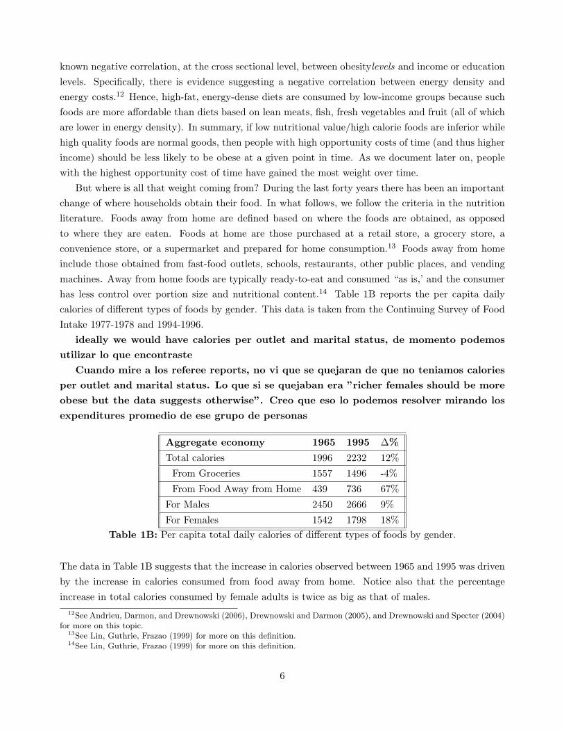
But where is all that weight coming from? During the last forty years there has been an importantchange of where households obtain their food. In what follows, we follow the criteria in the nutritionliterature. Foods away from home are defined based on where the foods are obtained, as opposedto where they are eaten. Foods at home are those purchased at a retail store, a grocery store, aconvenience store, or a supermarket and prepared for home consumption.13 Foods away from homeinclude those obtained from fast-food outlets, schools, restaurants, other public places, and vendingmachines. Away from home foods are typically ready-to-eat and consumed “as is,’ and the consumerhas less control over portion size and nutritional content.14 Table 1B reports the per capita dailycalories of different types of foods by gender. This data is taken from the Continuing Survey of FoodIntake 1977-1978 and 1994-1996.

ideally we would have calories per outlet and marital status, de momento podemos

utilizar lo que encontraste

Cuando mire a los referee reports, no vi que se quejaran de que no teniamos calories

per outlet and marital status. Lo que si se quejaban era ”richer females should be more

obese but the data suggests otherwise”. Creo que eso lo podemos resolver mirando los

expenditures promedio de ese grupo de personas

Aggregate economy 1965 1995 ∆%

Total calories 1996 2232 12%

From Groceries 1557 1496 -4%

From Food Away from Home 439 736 67%

For Males 2450 2666 9%

For Females 1542 1798 18%Table 1B: Per capita total daily calories of different types of foods by gender.

The data in Table 1B suggests that the increase in calories observed between 1965 and 1995 was drivenby the increase in calories consumed from food away from home. Notice also that the percentageincrease in total calories consumed by female adults is twice as big as that of males.

12See Andrieu, Darmon, and Drewnowski (2006), Drewnowski and Darmon (2005), and Drewnowski and Specter (2004)for more on this topic.

13See Lin, Guthrie, Frazao (1999) for more on this definition.14See Lin, Guthrie, Frazao (1999) for more on this definition.

6

To further explore what component of food away from home is the most important, Nielsen, Siega-Riz and Popkin (2002) further dissagregate the types of food and their origin. These authors studythe trends in locations and food sources of Americans stratified by age group for both total energyand the meal and snack subcomponents. Their findings are summarized in Table 1C.

Type of Food 1977-78 1994-96 ∆%

Meals

19-39 YearsAt Home 73 56.8 %

Away from Home 27 43.2 %

40-59 YearsAt Home 78.2 66.1 %

Away from Home 21.8 33.9 %

Snacks

19-39 YearsAt Home 10 12.2 %

Away from Home 90 87.8 %

40-59 YearsAt Home 76.9 70.8 %

Away from Home 23.1 29.2 %Table 1C: Trends in energy intake by eating ocasion and location (% energy).

Although all age groups have increased their consumption of meals from restaurants/fast-foodestablishments, the 19 to 39 year-olds have consumed the greatest percentage of restaurant/fast-foodmeals. In 1996, snacks from the store eaten out represented up to 12.2% of all energy from snacks,whereas meals from the store eaten out represented only up to 5.6% of all energy from meals for thisage group. It seems then that only snacks are not going to account most of the increase in obesityrates in the U.S.

The idea that lower food costs are behind recent obesity trends is pervasive in the empirical liter-ature. A prominent example is Cutler, Glaeser, and Shapiro (2003) who conclude that a technologicalrevolution in the mass preparation of food translated into a dramatic decline in the time cost andmarket price of food, particularly of mass prepared foods. The lower time cost and increased avail-ability of processed foods are, according to these authors, key factors behind the dramatic decline incooking times and home meals, and also behind the higher consumption of processed food, which mayaccount for the observed increase in caloric intake.

For completeness, we report in Figure 1 the trends in existing data on the price of groceries (labeledfood for off-premise consumption in the U.S. NIPA), and the price of food prepared away from homerelative to the GDP deflator. The relative price of groceries declined almost monotonically from 1955until 1973 when it jumped up by almost 15%. It remained high all through the mid 1970s and early

7

Prices relative to the GDP deflator

0.7

0.8

0.9

1.0

1.1

1.2

1959 1964 1969 1974 1979 1984 1989 1994 1999 2004

Food in Purchased Meals Food purchased for off-premise consumption

Figure 1: Price of food relative to the GDP deflator.

1980s. By 1982 the relative price of groceries was back at its 1972 level. From 1982 to the presentthis price has remained relatively constant. On the other hand, the aggregate price of food away fromhome has increased over the period examined. Of course, aggregate price indexes reported by the U.S.NIPA may not fully adjust for changes in portion sizes, nor quality. Data on changes in portion size ofthe aggregate “food prepared away from home” through time is not available. Given that Young andNestle (2002) find evidence that there has been substantial increase and variance regarding portionsize of many processed food items since the 1970s, we cannot make precise quantitative assessmentsof the price of food away from home.

2.2 Trends in macroeconomic observables

The idea that changes in opportunity cost are behind lower costs of processed food is consistent withthe findings of Prochaska and Schrimper (1973), who established a high positive correlation betweendifferent measures of opportunity cost of the household manager and the expenditure and frequencyof consumption in meals prepared away from home.15 Moreover, Jensen and Yen (1996) find that theeffects of a wife’s employment are significant and positive on both the consumption frequency andlevel of expenditure on lunch and dinner consumed away from home.16

15See Byrne, Capps, and Saha (1996), and Dong, Byrne, Saha and Capps (2000) for more recent analysis.16Similarly, Mutlua and Gracia (2006) find that income, household characteristics and the opportunity cost of women’s

time are important factors determining food consumption patterns away from home in Spain. Moreover, income and

8

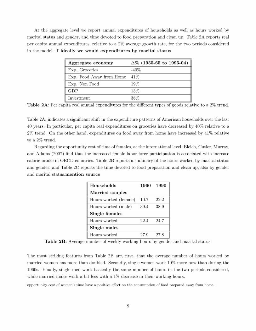
At the aggregate level we report annual expenditures of households as well as hours worked bymarital status and gender, and time devoted to food preparation and clean up. Table 2A reports realper capita annual expenditures, relative to a 2% average growth rate, for the two periods consideredin the model. T ideally we would expenditures by marital status

Aggregate economy ∆% (1955-65 to 1995-04)

Exp. Groceries -40%

Exp. Food Away from Home 41%

Exp. Non Food 19%

GDP 13%

Investment 38%Table 2A: Per capita real annual expenditures for the different types of goods relative to a 2% trend.

Table 2A, indicates a significant shift in the expenditure patterns of American households over the last40 years. In particular, per capita real expenditures on groceries have decreased by 40% relative to a2% trend. On the other hand, expenditures on food away from home have increased by 41% relativeto a 2% trend.

Regarding the opportunity cost of time of females, at the international level, Bleich, Cutler, Murray,and Adams (2007) find that the increased female labor force participation is associated with increasecaloric intake in OECD countries. Table 2B reports a summary of the hours worked by marital statusand gender, and Table 2C reports the time devoted to food preparation and clean up, also by genderand marital status.mention source

Households 1960 1990

Married couples

Hours worked (female) 10.7 22.2

Hours worked (male) 39.4 38.9

Single females

Hours worked 22.4 24.7

Single males

Hours worked 27.9 27.8Table 2B: Average number of weekly working hours by gender and marital status.

The most striking features from Table 2B are, first, that the average number of hours worked bymarried women has more than doubled. Secondly, single women work 10% more now than during the1960s. Finally, single men work basically the same number of hours in the two periods considered,while married males work a bit less with a 1% decrease in their working hours.

opportunity cost of women’s time have a positive effect on the consumption of food prepared away from home.

9

Households 1965 1995

Married couples

Hours food prep. (female) 13.0 6.4

Hours food prep. (male) 1.2 1.7

Single females

Hours food prep. 7.0 3.8

Single males

Hours food prep. 2.1 2.1Table 2C: Average number of weekly hours devoted to food preparation and clean up by gender

and marital status.

With respect to time spent in food preparation and clean up, Table 2C reveals that the average numberof hours that married women devote to these activities has decreased by 50%. Similarly, single womenspent 45% less time preparing home food and cleaning up in 1995 than in 1965. Married men devotedan almost insignificant amount of time to food preparation activities during the 1960s (less than 11minutes per day). Married men devoted 30% more time to food preparation during the 1990s, but inabsolute terms the time they allocate to cooking is very small (15 minutes per day).

The data reported on Tables 2B and 2C play an important role in our analysis. The 1960s data isused to calibrate some of the parameters of the model. Moreover, Tables 2B and 2C are also used toconfront the 1990s time-use predictions from the model to the observations of the U.S. economy.

The size and nature of the “gender wage gap” has been well-documented, see Goldin (1990).Women working full-time earned on average 54% of what men earned in the 1960’s. This ratioremained relatively flat until the late 1970s and then rose to about 74% by 1997. The “gender wagegap” is difficult to interpret as it can either measure the direct effects of discrimination or differencesin unmeasured skills correlated with gender. To keep our analysis simple we take the data on the“gender wage gap” as given and introduce it into our model as a gender-specific tax. Similar resultscan be obtained in a model with endogenous skill differences by gender or glass ceilings; see Jones,Manuelli and McGrattan (2003).

One of the key mechanisms driving the shift in consumption and the increased obesity rates ofall households explored in this paper is the increased opportunity cost of cooking at home. Changesin taxes are going to be important and will be directly incorporated into the model as reported inTable 3. Household taxes in this table correspond to the effective marginal tax rates for the averagehousehold by marital status and gender; see the Appendix for more details.

10

Effective Tax Rates 1955-65 1995-04

Households

Labor income for married couples 22% 15%

Labor income for single females 22% 15%

Labor income for single males 22% 22%

Capital income 22% 15%

Firms

Profits 43% 35%

Social security contributions 1% 4%Table 3: Marginal corporate and personal income tax rates by gender and marital status.

The tax reform Act of the mid 1980s translated into a lowering of the personal income tax rate. In thecase of single men, however, the reduction in the tax rate did not change as much as other households inthe 1990s. On the other hand, single women and married households have seen their average marginaltax rates fall the most. Finally, taxes on profits have declined during our sample period, which in acompetitive equilibrium translates into higher rates of return for capital. All of these changes haveimportant implications on the opportunity cost of cooking at home for the different households.

The purpose of this paper is to account for the observed changes in the average weight of Ameri-can adults. The theoretical framework we employ links an increase in the opportunity cost of cookingat home with higher consumption of foods prepared away from home, and thus higher calorie con-sumption. This positive correlation between time changes in the opportunity cost of time and obesityrates implied by our theory is not inconsistent with the well known negative correlation, at the crosssectional level, between obesity levels and income or education levels. Specifically, there is evidencesuggesting a negative correlation between energy density and energy costs; see for example, Andrieu,Darmon, and Drewnowski (2006), Drewnowski and Darmon (2005), and Drewnowski and Specter(2004). Hence, high-fat, energy-dense diets are consumed by low-income groups because such foodsare more affordable than diets based on lean meats, fish, fresh vegetables and fruit (all of which arelower in energy density). In summary, if low nutritional value/high calorie foods are inferior whilehigh quality foods are normal goods, then people with high opportunity costs of time (and thus higherincome) should be less likely to be obese at a given point in time. As we document later on, peoplewith the highest opportunity cost of time have gained the most weight over time.

3 The Model

We consider a setting in which representative households –single women, single men, and marriedcouples– must decide how to allocate their labor endowments across market activities and the pro-duction of food at home taking the prices of food as given. Households must also decide how muchto spend on groceries for cooking food at home, on meals prepared outside the home and on othernon-food items. We make the simplifying assumption that agents choose the types of meals they

11

consume (prepared at home from scratch or away) but not the number of calories they consume. Allhouseholds face a common set of technological restrictions, and each is taxed on the income earned inthe market sector. We model the gender wage gap as a tax wedge that differs by gender. Householdsare the owners of capital, and they rent it to firms at a competitively determined interest rate.

Married Households

We now present the problem of a representative married couple, or partnership. We assume that thebargaining problem within the household is resolved efficiently, so that a weighted form of a planner’sproblem describes the decisions that the couple makes. The preferences of such a partnership overconsumption of food, CF , other consumption goods, CNF , and leisure streams, L̂− Lh − Lm, can berepresented by:

∑t

βt

1− σ{λf

(α(CpfF,t)

1−σ + ν (CpfNF,t)1−σ + (1− α− ν)

(L̂− Lpfh,t − L

pfm,t

)1−σ)

+ (1)

(1− λf )(α (CpmF,t )

1−σ + ν (CpmNF,t)1−σ + (1− α− ν)

(L̂− Lpmh,t − L

pmm,t

)1−σ)};

where the first superscript p indicates partnership and the second indicates the type within the house-hold; i.e., f (m) for female (male); the subscripts m, and h stand for market and household activitiesrespectively and the subscript t represents time. Agents in this economy have an endowment of L̂hours.17 The relative weight of the woman’s utility in a partnership is λf , β is the discount factor, ndenotes the population growth rate and σ, α and ν are preference parameters.

The problem of the partnership is to maximize equation (1) subject to several constraints. First,total food consumption in the married household, CpF , obtained through foods prepared away fromhome (F p) and home meals (HF p), is given by:

CpF,t = CpfF,t + CpmF,t =(µ1 (F pt )γ + (1− µ1) (HF pt )γ

)1/γ ; (2)

where γ denotes the degree of substitution between foods prepared away from home and home preparedmeals, and µ1 represents the relative importance of food away from home. Home meals are producedusing groceries, Ip, together with female and male cooking labor, Lpfh and Lpmh , respectively. Weassume that time is complementary with groceries in the production of food. In particular, we have:

HF p = min[Ip, ζ0(Lpfh )ζ1(Lpmh )1−ζ1

]; (3)

where ζ1 is the share of female cooking hours and ζ0 is a conversion factor between groceries and laborcooking hours.

Consumption goods other than food are acquired in the market. Total consumption of non food17Time-use studies show that Americans sleep 8 hours per day [14]. During the average day, 1 hour of time is used

for eating and 1 hour for obtaining goods and services. Therefore, we assume each individual has 14 hours available perday, or L̂=5488 hours per year.

12

items of the partnership is denoted by:

NF pt = CpfNF,t + CpmNF,t. (4)

Households can also invest in the capital stock used in market activities, kpm, as well as in capitalspecific for the food away from home sector, kpf . These capitals evolve over time according to:

kpm,t+1 = Xpm,t + (1− δ)kpm,t (5)

kpf,t+1 = Xpf,t + (1− δ)kpf,t; (6)

where X represents investment, and δ denotes the depreciation rate. Finally, households face thetypical budget constraint given by:

PF,tFpt +NF pt + Ipt +Xp

m,t +Xpf,t +Rtb

pt ≤ (7)

(1− τp)(wt((1− τd)Lpfm,t + Lpmm,t)

)+ (1− τk) {(1− τc)(rt+1 − δ) + δ}[kpm,t + kpf,t] + bpt+1 + T pt

where Lp,jm denotes hours devoted to market activities by the members in the partnership for j=f,m;bp are bond holdings, τp denotes the tax on labor income, (1− τd) denotes the gender wage gap tax,and PF corresponds to the price of food away from home relative to the GDP deflator. FollowingHayashi (1982) and McGrattan and Prescott (2005), we map profits in the data to capital income inour model.18 The tax rate on profits is denoted by τc. The tax rate on capital income, τk, is assumedto be common for single and married agents households. The latter is a technical condition requiredso that all households hold a positive amount of capital in equilibrium.

We assume the relative price of groceries equal to one, as data shows no significant change overthe periods we consider. The wage rate is denoted by w, r corresponds to the rental rate on capital,R is the return on bonds, T p are taxes rebated to households as lump sum transfers. To guaranteethat the problem of the household is well defined, we restrict borrowing to be less than the presentvalue of future wealth. Such a constraint does not bind along the balanced growth path.

Finally, this economy is also populated by representative single male and female households whosepreferences and optimization problems are analogous to the partnership’s problem.19

Technological Constraints and Aggregate Feasibility

Our economy has two representative competitive firms. One produces food away from home usingcapital and labor. Its production technology can be represented by:

Kθf

f (AfLf )1−θf.

18Alternatively, one can write a model where firms are the owners of capital and pay dividends to households. Such amodel results in equilibrium allocations identical to ours.

19The problem of the single female can be derived from the married households problem by setting λf = 1, and ζ1 = 1.Similarly, the problem of the single male sets λm = 1, and ζ1 = 0.

13

The other representative firm produces non-food goods, investment and services with the Cobb-Douglas technology

Kθmm (AmLm)1−θm

.

In the above equations Ki, Ai, Li and θi denote the capital, productivity, labor and capital share insector i=m, f . Firms produce and rent productive inputs taking prices as given. Constant returns toscale in a competitive framework implies zero profits for each one of the representative firms. Moreover,rental rates must equal marginal products, namely:

r = θfKθf−1f (AfLf )1−θf = θmK

θm−1m (AmLm)1−θm

, and

w (1 + τss) = (1− θf )Kθf

f (AfLf )−θf = (1− θm)Kθmm (AmLm)−θm

.

where firms are required to make social security contributions at rate τss.Market clearing in the food away from home sector requires that the demand of food away from

home of all households, F , is equal to the available production. Namely:

F = Kθf

f (AfLf )1−θf.

Similarly, market clearing in the second sector of the economy implies

NF + I +Xm +Xf = Kθmm (AmLm)1−θm

.

In the previous market clearing conditions, capital letters with no super-index denote the corre-sponding aggregate variable (weighted by the fraction of the population).

Equilibrium

A competitive equilibrium for this economy is a sequence of prices and allocations for the partner-ship, single households, and firms that solve the corresponding optimization problems, taking prices asgiven. For it to be equilibrium all of the aggregate resource constraints and market clearing conditionsmust also be satisfied. A balanced growth equilibrium is an equilibrium where expenditures grow atconstant rates and time use variables remain constant through time.

3.1 Some Theoretical Predictions

A closed-form solution for all equilibrium variables of this model cannot be obtained, except for veryspecific parameterizations. In this section we characterize the equilibrium behavior of some of thekey variables of the model. Our purpose is to develop the economic intuition of the forces drivingour results, which will help in obtaining a better understanding of the quantitative findings that wederive, numerically, in the following sections of the paper.

14

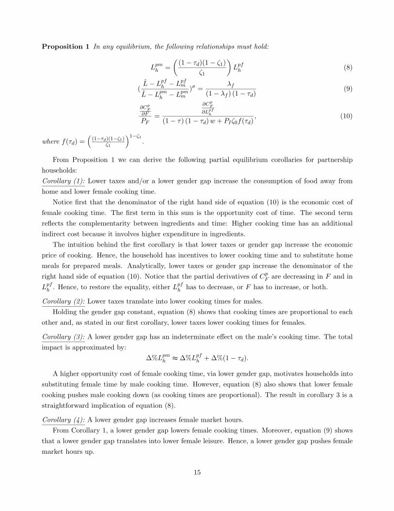
Proposition 1 In any equilibrium, the following relationships must hold:

Lpmh =(

(1− τd)(1− ζ1)ζ1

)Lpfh (8)

(L̂− Lpfh − L

pfm

L̂− Lpmh − Lpmm

)σ =λf

(1− λf ) (1− τd)(9)

∂CpF

∂F

PF=

∂CpF

∂Lpfh

(1− τ) (1− τd)w + PIζ0f(τd), (10)

where f(τd) =(

(1−τd)(1−ζ1)ζ1

)1−ζ1.

From Proposition 1 we can derive the following partial equilibrium corollaries for partnershiphouseholds:Corollary (1): Lower taxes and/or a lower gender gap increase the consumption of food away fromhome and lower female cooking time.

Notice first that the denominator of the right hand side of equation (10) is the economic cost offemale cooking time. The first term in this sum is the opportunity cost of time. The second termreflects the complementarity between ingredients and time: Higher cooking time has an additionalindirect cost because it involves higher expenditure in ingredients.

The intuition behind the first corollary is that lower taxes or gender gap increase the economicprice of cooking. Hence, the household has incentives to lower cooking time and to substitute homemeals for prepared meals. Analytically, lower taxes or gender gap increase the denominator of theright hand side of equation (10). Notice that the partial derivatives of CpF are decreasing in F and inLpfh . Hence, to restore the equality, either Lpfh has to decrease, or F has to increase, or both.

Corollary (2): Lower taxes translate into lower cooking times for males.Holding the gender gap constant, equation (8) shows that cooking times are proportional to each

other and, as stated in our first corollary, lower taxes lower cooking times for females.

Corollary (3): A lower gender gap has an indeterminate effect on the male’s cooking time. The totalimpact is approximated by:

∆%Lpmh ≈ ∆%Lpfh + ∆%(1− τd).

A higher opportunity cost of female cooking time, via lower gender gap, motivates households intosubstituting female time by male cooking time. However, equation (8) also shows that lower femalecooking pushes male cooking down (as cooking times are proportional). The result in corollary 3 is astraightforward implication of equation (8).

Corollary (4): A lower gender gap increases female market hours.From Corollary 1, a lower gender gap lowers female cooking times. Moreover, equation (9) shows

that a lower gender gap translates into lower female leisure. Hence, a lower gender gap pushes femalemarket hours up.

15

As the previous corollaries illustrate, changes in taxes and the gender wage gap are key elementsin explaining the increased opportunity cost of cooking at home. These theoretical results also showthat changes in taxes and in the gender wage gap are not symmetric in terms of their effects on theopportunity costs faced by men and women. Changes in taxes affect both genders in a similar fashion.On the other hand, a change in the gender wage gap directly affects the opportunity cost of women.This asymmetry is especially important for married households since it implies different degrees ofspecialization in home production. Moreover, it can also help explain the different consumption andleisure patterns observed among the different single female and single male households.

In the next sections, we describe and perform the quantitative analysis. Our numerical resultsreveal that the channels presented in this section are also observed when all general equilibrium effectsare considered.

3.2 Calibration

We set the values of the parameters so that the balanced growth equilibrium time series match some oftheir counterparts in the U.S. data during the period 1955-65. Estimates of the intertemporal elasticityof substitution found in the macroeconomic literature imply values for σ within the interval [1,2]. Inour baseline experiment we set a value of σ = 1.5. Some parameters of the model are straightforwardto calibrate. We set the depreciation rate for capital at 6%, the discount factor β so that the interestrate matches the average 4% in the data. The parameter of the aggregate production function for themarket good, θm, is set so that the share of income going to labor from the model matches its datacounter part, θm=0.34. Similarly, parameter θf is such that the model matches the capital-labor ratioof the restaurant industry, which results in θf=0.08. The growth factor of the exogenous technologyparameter for the numeraire good is set at 1.02 so that the model matches the average growth rate ofper-capita GDP of the U.S. economy.

There is a large body of empirical literature devoted to the analysis of food consumption choicesof American households. A recent study by Piggot (2003) develops a nested empirical model includingmost of the commonly employed demand systems for food in the United States. The author reportsvalues for the price elasticity of food away from home that range between -2.3 and -1.16. In our model,the price elasticity of food away from home is determined by parameter γ. We set at γ = 0.87 to matchthe middle point of the values reported by Piggot, i.e. a price elasticity of food of −1.73.

Regarding married households, there are six parameters left to be calibrated: the weights in theutility of food and non-food consumption goods, which are given by α, ν, respectively; the weightof the female in the total household utility in the married household, given by λf ; and a set offood technology parameters µ, ζ0, and ζ1. The values of these parameters are jointly determined fromsteady state equations so that the model matches six U.S. averages for 1955-65. In particular, wematch the hours worked and hours preparing food from Tables 2A and 2B (4 observations for marriedhouseholds), a ratio of aggregate expenditure in consumption other than food to food away from home

16

equal to 18, and a ratio of aggregate expenditure in ingredients to food away from home of 3.20 Thefour parameters associated to the single households (α, ν, µ, ζ0)s,i are calibrated to match hours workedand preparing food of single adults (two observations each) and the two ratios of aggregate data usedfor married households.

3.3 Results

In this section we perform a quantitative analysis of two different mechanisms that lower the relativecost of food prepared away from home, which may help understanding the increased weight of Americanadults. All experiments depart from a common balanced growth path that we associate to the 1955-65U.S. economy. We study each channel independently. First, we hold income taxes and the genderwage gap constant and feed into the model an exogenous increase in the productivity of producingfood away from home. Finally, we feed into the model the observed trends in income taxes andthe gender wage gap, holding the productivity of the food away from home sector constant. Wecompute the balanced growth equilibrium associated to each one of these changes and assume thisnew equilibrium corresponds to the 1995-04 U.S. data. We then derive the quantitative implications ofthese mechanisms and compare the predictions of the model to their data counterparts in the followingdimensions: aggregate expenditure in food prepared away from home, in ingredients for preparing foodat home, in non-food consumption, time use, and a set of key macroeconomic aggregates like GDP andInvestment. We consider GDP and Investment because the two channels that we are examining havestrong implications for these two macroeconomic aggregates. In particular, changes in productivitydirectly affect the rates of return and in turn affect investment. Similarly, a decrease in taxes increasesthe after tax return thus directly affecting investment.

3.3.1 Changes in the production technology of food away from home

Technological advancements in the production of food prepared away from home that result in lowerprices are a common explanation for the observed trends in consumption of food prepared away fromhome, food at home, and cooking times. We use our model to derive the quantitative implications ofthis mechanism.

We capture technological improvements in the food away from home sector by introducing asequence of productivity parameters, AF , that grows faster than the overall growth rate of total factorproductivity during our sample period.21 An increase in the productivity of the food prepared awayfrom home sector increases its supply, which results in a lower price. Lower prices for foods prepared

20Consumption other than food is measured from the NIPA as Nondurable consumption expenditure + Governmentexpenditure + Net exports – Food expenditure (the latter from the detailed personal consumption expenditure tables ofthe BEA). Ingredients correspond to food purchased for off premise consumption in the detailed personal consumptionexpenditure tables of the BEA.

21Data on the capital stock, hours worked, and value added for the food away from home sector is available in the U.S.NIPA from 1987 to the present. A measure for AF based on such data, and on the corresponding production functionof our model, shows productivity in this sector growing slightly below 2% per year. Measured output in the food awayfrom home sector is subject to biases from changes in portion size and quality. Thus, we have chosen values of AF basedon existing hypotheses and to explore its quantitative implications.

17

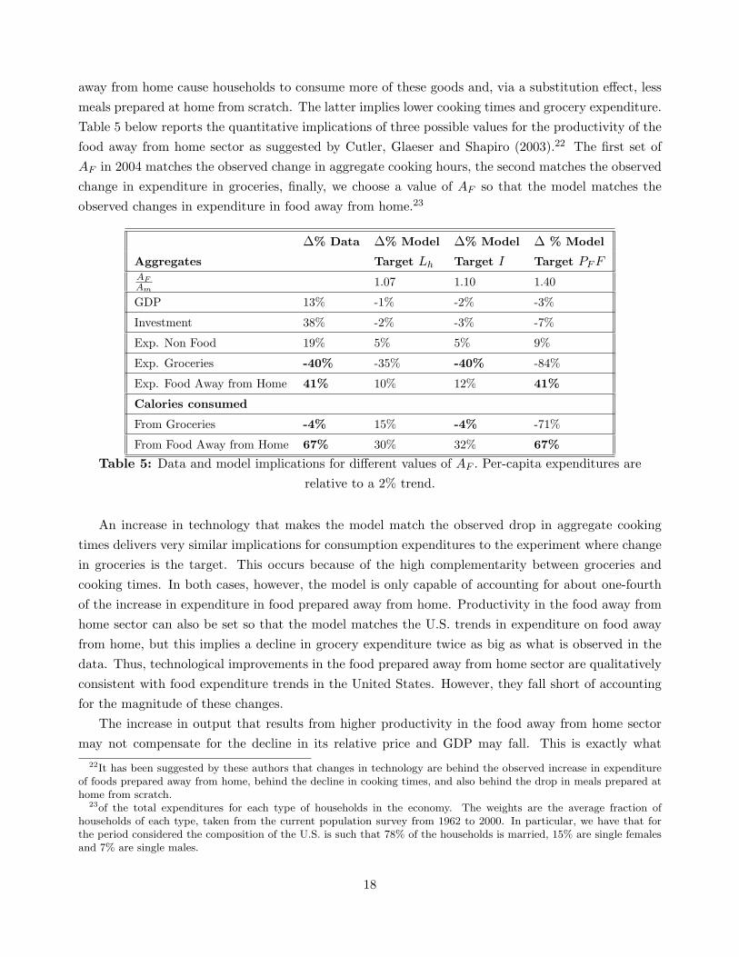
away from home cause households to consume more of these goods and, via a substitution effect, lessmeals prepared at home from scratch. The latter implies lower cooking times and grocery expenditure.Table 5 below reports the quantitative implications of three possible values for the productivity of thefood away from home sector as suggested by Cutler, Glaeser and Shapiro (2003).22 The first set ofAF in 2004 matches the observed change in aggregate cooking hours, the second matches the observedchange in expenditure in groceries, finally, we choose a value of AF so that the model matches theobserved changes in expenditure in food away from home.23

∆% Data ∆% Model ∆% Model ∆ % Model

Aggregates Target Lh Target I Target PFFAFAm

1.07 1.10 1.40

GDP 13% -1% -2% -3%

Investment 38% -2% -3% -7%

Exp. Non Food 19% 5% 5% 9%

Exp. Groceries -40% -35% -40% -84%

Exp. Food Away from Home 41% 10% 12% 41%

Calories consumed

From Groceries -4% 15% -4% -71%

From Food Away from Home 67% 30% 32% 67%

Table 5: Data and model implications for different values of AF . Per-capita expenditures arerelative to a 2% trend.

An increase in technology that makes the model match the observed drop in aggregate cookingtimes delivers very similar implications for consumption expenditures to the experiment where changein groceries is the target. This occurs because of the high complementarity between groceries andcooking times. In both cases, however, the model is only capable of accounting for about one-fourthof the increase in expenditure in food prepared away from home. Productivity in the food away fromhome sector can also be set so that the model matches the U.S. trends in expenditure on food awayfrom home, but this implies a decline in grocery expenditure twice as big as what is observed in thedata. Thus, technological improvements in the food prepared away from home sector are qualitativelyconsistent with food expenditure trends in the United States. However, they fall short of accountingfor the magnitude of these changes.

The increase in output that results from higher productivity in the food away from home sectormay not compensate for the decline in its relative price and GDP may fall. This is exactly what

22It has been suggested by these authors that changes in technology are behind the observed increase in expenditureof foods prepared away from home, behind the decline in cooking times, and also behind the drop in meals prepared athome from scratch.

23of the total expenditures for each type of households in the economy. The weights are the average fraction ofhouseholds of each type, taken from the current population survey from 1962 to 2000. In particular, we have that forthe period considered the composition of the U.S. is such that 78% of the households is married, 15% are single femalesand 7% are single males.

18

happens in the quantitative experiments reported in Table 5 where GDP declines by at least 1%, andinvestment by at least 3% relative to a 2% trend. These two predictions are not consistent with U.S.data where per capita GDP increased by 13%, and investment by 38% relative to a 2% trend. In all ofthe experiments we consider, changes in technology fall short of accounting for the observed increasein aggregate expenditure on non-food consumption items.

In order to obtain the implications of the model regarding calorie consumption we perform thefollowing procedure. First, we derive from the U.S. data a transformation factor mapping dollars spentinto calories consumed for each type of food. This transformation factor is such that the observedchange in real per capita expenditures is compatible with the observed change in calorie consumptionfrom the data. Finally, we apply the same transformation factor to the expenditures obtained in themodel and derive the calories consumed implied by the theory. Using this procedure, Table 5 showsthat technological advancements in the production of foods prepared away from home when we targetaggregate hours predict more than half of the caloric increase due to food away from home and isqualitatively inconsistent with the observed decrease in calories from home cooked meals. When thetarget is expenditures on ingredients the model can only account for half of the calories of food awayfrom home and by construction all of the caloric decrease in home cooked meals. Finally, when thetarget are the expenditures of food away from home, the model over states the decrease in caloriesfrom home cooked meals by almost a factor of two, and by construction matches all of the caloricincrease from food away from home. Note that we have divided total calorie consumption by sourceof preparation (at home from scratch vs. prepared away from home). Cutler, Glaeser and Shapiro(2003) divide calorie consumption by the different meals and snacks of a given day, and find that mostof the increase in calorie consumption can be attributed to snacks, which according to the authors,are largely pre-prepared. Thus, these two breakdowns are consistent with each other.

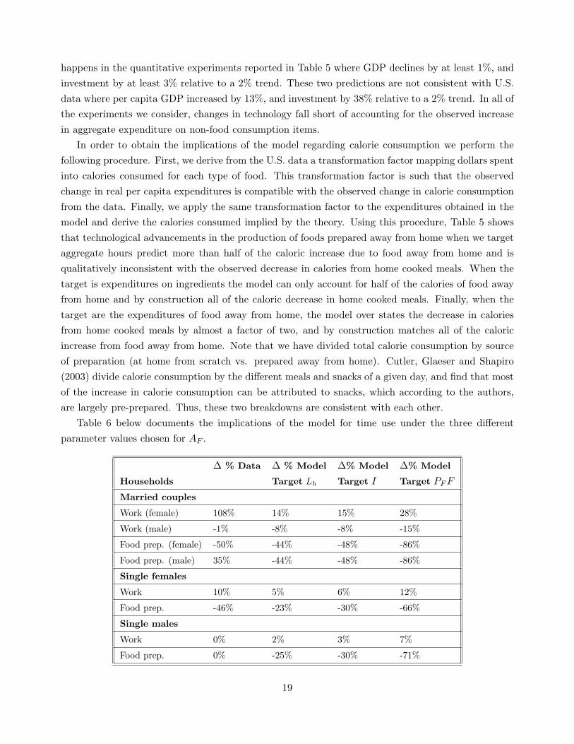
Table 6 below documents the implications of the model for time use under the three differentparameter values chosen for AF .

∆ % Data ∆ % Model ∆% Model ∆% Model

Households Target Lh Target I Target PFF

Married couples

Work (female) 108% 14% 15% 28%

Work (male) -1% -8% -8% -15%

Food prep. (female) -50% -44% -48% -86%

Food prep. (male) 35% -44% -48% -86%

Single females

Work 10% 5% 6% 12%

Food prep. -46% -23% -30% -66%

Single males

Work 0% 2% 3% 7%

Food prep. 0% -25% -30% -71%

19

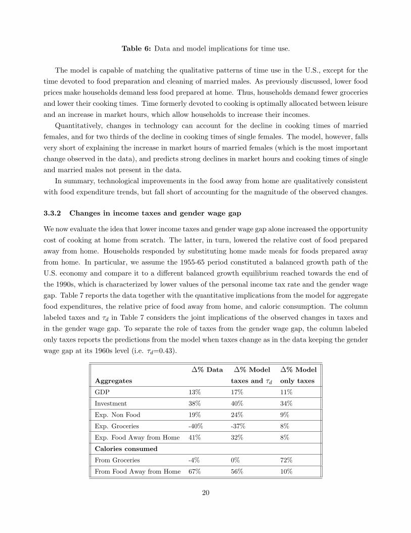
Table 6: Data and model implications for time use.

The model is capable of matching the qualitative patterns of time use in the U.S., except for thetime devoted to food preparation and cleaning of married males. As previously discussed, lower foodprices make households demand less food prepared at home. Thus, households demand fewer groceriesand lower their cooking times. Time formerly devoted to cooking is optimally allocated between leisureand an increase in market hours, which allow households to increase their incomes.

Quantitatively, changes in technology can account for the decline in cooking times of marriedfemales, and for two thirds of the decline in cooking times of single females. The model, however, fallsvery short of explaining the increase in market hours of married females (which is the most importantchange observed in the data), and predicts strong declines in market hours and cooking times of singleand married males not present in the data.

In summary, technological improvements in the food away from home are qualitatively consistentwith food expenditure trends, but fall short of accounting for the magnitude of the observed changes.

3.3.2 Changes in income taxes and gender wage gap

We now evaluate the idea that lower income taxes and gender wage gap alone increased the opportunitycost of cooking at home from scratch. The latter, in turn, lowered the relative cost of food preparedaway from home. Households responded by substituting home made meals for foods prepared awayfrom home. In particular, we assume the 1955-65 period constituted a balanced growth path of theU.S. economy and compare it to a different balanced growth equilibrium reached towards the end ofthe 1990s, which is characterized by lower values of the personal income tax rate and the gender wagegap. Table 7 reports the data together with the quantitative implications from the model for aggregatefood expenditures, the relative price of food away from home, and caloric consumption. The columnlabeled taxes and τd in Table 7 considers the joint implications of the observed changes in taxes andin the gender wage gap. To separate the role of taxes from the gender wage gap, the column labeledonly taxes reports the predictions from the model when taxes change as in the data keeping the genderwage gap at its 1960s level (i.e. τd=0.43).

∆% Data ∆% Model ∆% Model

Aggregates taxes and τd only taxes

GDP 13% 17% 11%

Investment 38% 40% 34%

Exp. Non Food 19% 24% 9%

Exp. Groceries -40% -37% 8%

Exp. Food Away from Home 41% 32% 8%

Calories consumed

From Groceries -4% 0% 72%

From Food Away from Home 67% 56% 10%

20

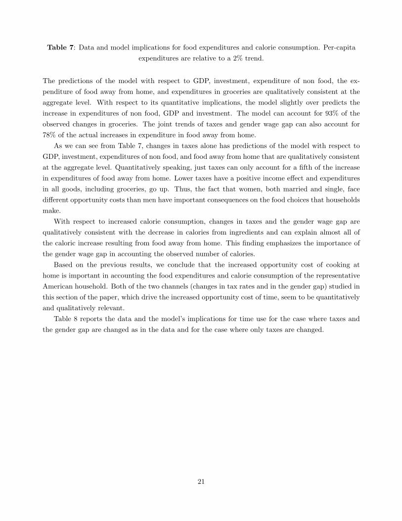
Table 7: Data and model implications for food expenditures and calorie consumption. Per-capitaexpenditures are relative to a 2% trend.

The predictions of the model with respect to GDP, investment, expenditure of non food, the ex-penditure of food away from home, and expenditures in groceries are qualitatively consistent at theaggregate level. With respect to its quantitative implications, the model slightly over predicts theincrease in expenditures of non food, GDP and investment. The model can account for 93% of theobserved changes in groceries. The joint trends of taxes and gender wage gap can also account for78% of the actual increases in expenditure in food away from home.

As we can see from Table 7, changes in taxes alone has predictions of the model with respect toGDP, investment, expenditures of non food, and food away from home that are qualitatively consistentat the aggregate level. Quantitatively speaking, just taxes can only account for a fifth of the increasein expenditures of food away from home. Lower taxes have a positive income effect and expendituresin all goods, including groceries, go up. Thus, the fact that women, both married and single, facedifferent opportunity costs than men have important consequences on the food choices that householdsmake.

With respect to increased calorie consumption, changes in taxes and the gender wage gap arequalitatively consistent with the decrease in calories from ingredients and can explain almost all ofthe caloric increase resulting from food away from home. This finding emphasizes the importance ofthe gender wage gap in accounting the observed number of calories.

Based on the previous results, we conclude that the increased opportunity cost of cooking athome is important in accounting the food expenditures and calorie consumption of the representativeAmerican household. Both of the two channels (changes in tax rates and in the gender gap) studied inthis section of the paper, which drive the increased opportunity cost of time, seem to be quantitativelyand qualitatively relevant.

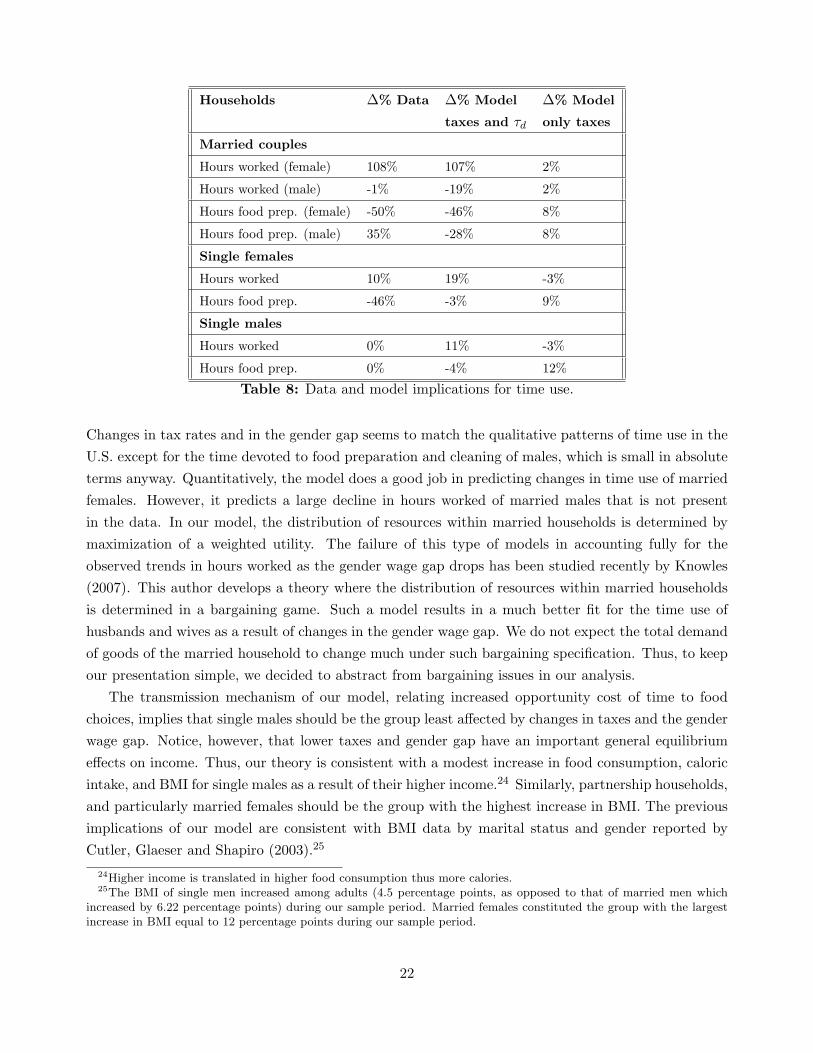
Table 8 reports the data and the model’s implications for time use for the case where taxes andthe gender gap are changed as in the data and for the case where only taxes are changed.

21

Households ∆% Data ∆% Model ∆% Model

taxes and τd only taxes

Married couples

Hours worked (female) 108% 107% 2%

Hours worked (male) -1% -19% 2%

Hours food prep. (female) -50% -46% 8%

Hours food prep. (male) 35% -28% 8%

Single females

Hours worked 10% 19% -3%

Hours food prep. -46% -3% 9%

Single males

Hours worked 0% 11% -3%

Hours food prep. 0% -4% 12%

Table 8: Data and model implications for time use.

Changes in tax rates and in the gender gap seems to match the qualitative patterns of time use in theU.S. except for the time devoted to food preparation and cleaning of males, which is small in absoluteterms anyway. Quantitatively, the model does a good job in predicting changes in time use of marriedfemales. However, it predicts a large decline in hours worked of married males that is not presentin the data. In our model, the distribution of resources within married households is determined bymaximization of a weighted utility. The failure of this type of models in accounting fully for theobserved trends in hours worked as the gender wage gap drops has been studied recently by Knowles(2007). This author develops a theory where the distribution of resources within married householdsis determined in a bargaining game. Such a model results in a much better fit for the time use ofhusbands and wives as a result of changes in the gender wage gap. We do not expect the total demandof goods of the married household to change much under such bargaining specification. Thus, to keepour presentation simple, we decided to abstract from bargaining issues in our analysis.

The transmission mechanism of our model, relating increased opportunity cost of time to foodchoices, implies that single males should be the group least affected by changes in taxes and the genderwage gap. Notice, however, that lower taxes and gender gap have an important general equilibriumeffects on income. Thus, our theory is consistent with a modest increase in food consumption, caloricintake, and BMI for single males as a result of their higher income.24 Similarly, partnership households,and particularly married females should be the group with the highest increase in BMI. The previousimplications of our model are consistent with BMI data by marital status and gender reported byCutler, Glaeser and Shapiro (2003).25

24Higher income is translated in higher food consumption thus more calories.25The BMI of single men increased among adults (4.5 percentage points, as opposed to that of married men which

increased by 6.22 percentage points) during our sample period. Married females constituted the group with the largestincrease in BMI equal to 12 percentage points during our sample period.

22

We can conclude then that lower taxes and the narrowing of the gender wage gap between maleand female workers are important elements when accounting for the increased calorie consumptionover the last 40 years in the U.S. In particular, the asymmetric nature of the gender wage gap is anecessary component when explaining the observed specialization in home production within marriedhouseholds as well as the different consumption and leisure patterns observed between single male andfemale households.

3.3.3 Further discussion

American households have substituted food prepared from scratch at home for food prepared awayfrom home. Moreover, according to dietary studies people end up consuming more calories when eatingfood prepared away from home. An interesting question is why, in equilibrium, food prepared awayfrom home has not become more similar to food prepared at home from scratch. Certain observationssuggest that changes in technology in the food away from home sector have favored the productionof calorie-intensive foods relative to healthier foods (or at least higher prices for foods prepared awayfrom home that are also healthier). First, technical change in the preparation of mass produced foodshas contributed to widen the gap between the price of healthier foods and calorie dense foods overtime.26 The widespread use of hydrogenated oils constitutes one of the examples of technologicaladvancements that favored high calorie food.27 The greater the degree of hydrogenation, the moresaturated the fat becomes. Benefits of hydrogenating plant-based fats for food manufacturers includean increased product shelf life and decreased refrigeration requirement. Plant-based hydrogenatedvegetable oils are much less expensive than the animal fats traditionally favored by bakers, such asbutter or lard, and may be more readily available than semi-solid plant fats such as palm oil. Finally,partially hydrogenated oils spoil and break down less easily under conditions of high temperatureheating. This is why they are used in restaurants for deep frying, to reduce how often the oil must bechanged.

Certainly, many factors have to be included in a theory that fully accounts for the observedchanges in time use of the average American household, and its implications for obesity trends in theUnited States. For instance, our analysis has abstracted from self-control problems and changes insocial weight norms, which according to Heiland and Burke (2007) may help us better understand theobserved changes in the weight distribution of American adults. We also abstracted from changes thebargaining power of married women that result from a lower gender gap, as considered by Knowles(2007). Changes in bargaining power may help accounting for the fact that the amount of timemarried men devote to cooking activities has increased substantially since the 1960s (although it isvery small in absolute numbers). Our analysis has all agents working. Thus, our framework is notdesigned to address the fact that cooking times of non-working married women have declined sincethe 1960s. The latter observation may seem first at odds with the increased opportunity cost of time

26A typical example is the dramatic increase in the production of trans fats since the 1960s.27“Hydrogenate” means to add hydrogen or, in the case of fatty acids, to saturate. The process changes liquid oil,

naturally high in unsaturated fatty acids, to a more solid and more saturated form.

23

channel explored in this paper. It is important to note, nevertheless, that the characteristics of non-working married women have also changed dramatically through time, and that such changes mayaccount for the observed decline in cooking times. In particular, relative to the 1960s, the averagenon-working married women of today is out of the labor force only for a short period of time.28

Thus, non-working married women today have lower experience associated with household activities,including cooking. Furthermore, non-working married women today also devote larger amount oftime to childcare activities, leaving less time for cooking.29 Finally, changes in the relative wage ofwomen may substantially alter the division of labor within the household, as suggested by Albanesiand Olivetti (2006), which may translate into lower cooking times.

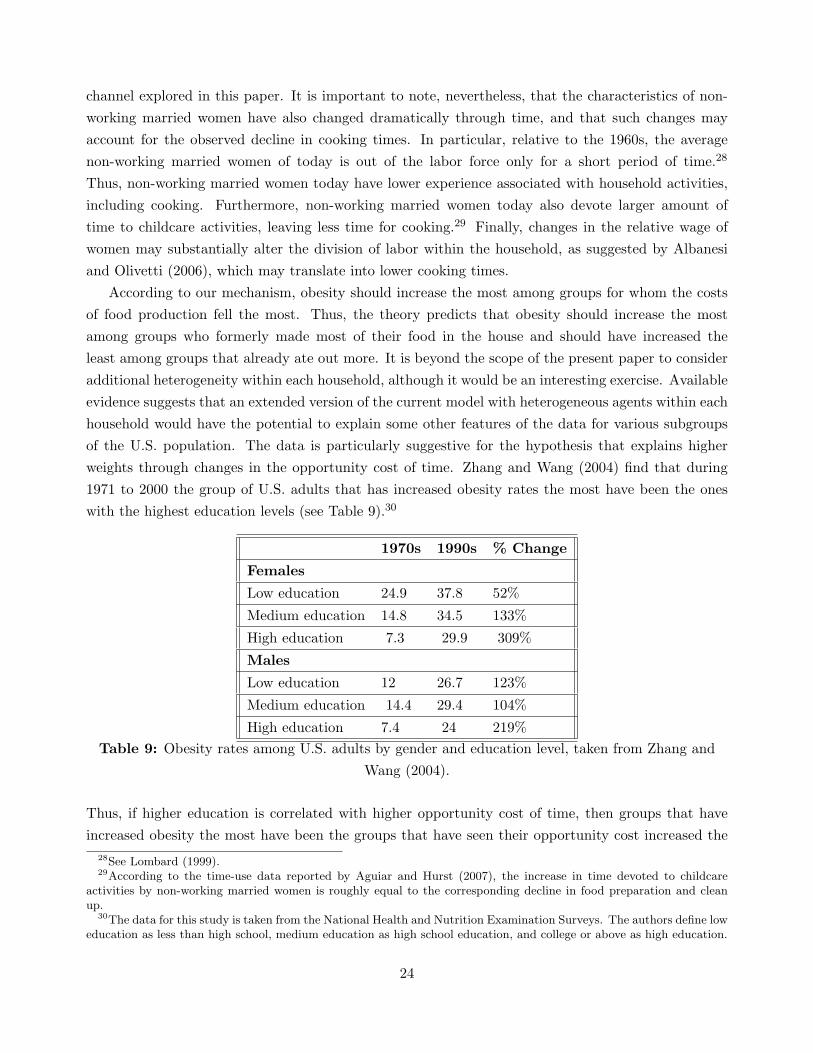
According to our mechanism, obesity should increase the most among groups for whom the costsof food production fell the most. Thus, the theory predicts that obesity should increase the mostamong groups who formerly made most of their food in the house and should have increased theleast among groups that already ate out more. It is beyond the scope of the present paper to consideradditional heterogeneity within each household, although it would be an interesting exercise. Availableevidence suggests that an extended version of the current model with heterogeneous agents within eachhousehold would have the potential to explain some other features of the data for various subgroupsof the U.S. population. The data is particularly suggestive for the hypothesis that explains higherweights through changes in the opportunity cost of time. Zhang and Wang (2004) find that during1971 to 2000 the group of U.S. adults that has increased obesity rates the most have been the oneswith the highest education levels (see Table 9).30

1970s 1990s % Change

Females

Low education 24.9 37.8 52%

Medium education 14.8 34.5 133%

High education 7.3 29.9 309%

Males

Low education 12 26.7 123%

Medium education 14.4 29.4 104%

High education 7.4 24 219%Table 9: Obesity rates among U.S. adults by gender and education level, taken from Zhang and

Wang (2004).

Thus, if higher education is correlated with higher opportunity cost of time, then groups that haveincreased obesity the most have been the groups that have seen their opportunity cost increased the

28See Lombard (1999).29According to the time-use data reported by Aguiar and Hurst (2007), the increase in time devoted to childcare

activities by non-working married women is roughly equal to the corresponding decline in food preparation and cleanup.

30The data for this study is taken from the National Health and Nutrition Examination Surveys. The authors define loweducation as less than high school, medium education as high school education, and college or above as high education.

24

most too. Furthermore, one of the main factors causing the increased weight of American adultssuggested by our theory is the observed decline in the gender wage gap. Blau (1998) finds that therelative gender wage gap for adults with low education levels has declined less than that of adultswith high education levels. The gender wage gap over 1969-1994 for individuals with less than 12years of education declined by 19.67%, while the one for more than 12 years of education declined by25%. Thus, the groups of individuals for which the gender wage gap has declined the most are alsothe groups where obesity rates have increased the most. These observations are consistent with thehypothesis that the increased opportunity cost of cooking at home is an important factor driving theincrease in obesity in the U.S. over the last forty years.

A puzzling observation that emerges from Table 9 is that, at the cross-sectional level, the groupsof people with higher education, income, and thus higher opportunity cost of time, are less likelyto be obese at a given point in time. It seems then important to discuss how this observation canbe reconciled with the transmission mechanism linking higher opportunity cost of time to higherconsumption of food prepared away from home, and to higher consumption of calories. The evidencein Andrieu, Darmon, and Drewnowski (2006) as well as in Drewnowski and Darmon (2005) illustratethat, at a given point in time, the price of foods with higher fat and calorie content is cheaper than thatof foods with lower calorie content and higher nutritional value. Thus, if low nutritional value/highcalorie foods are inferior while high quality foods are normal goods, then people with high opportunitycosts of time (and thus higher income) should be less likely to be obese at a given point in time.31

Notice, however, that people with the highest opportunity cost of time have gained the most weightover time. The latter fact suggests that the lower price of high calorie food brought by technologicalchange in the mass preparation of foods has dominated the income effect in determining the caloriccomposition of food away from home consumed by American household.

Regarding childhood obesity, Anderson, Butcher and Levine (2003) find that a child is more likelyto be overweight if her mother worked more intensively (more hours per week) over the child’s life.This effect is particularly evident for children of white mothers, of mothers of high education, and ofmothers with a high income level. This evidence is consistent with one of the mechanisms we haveevaluated since this increase in obesity may be due to the higher opportunity cost of cooking by theirmothers.

Finally, at the international level, Foreman-Peck, Humphries, Morris, Offer and Stead (1998) findthat increased obesity rates in Great Britain are correlated with the lowering of the gender gap andsubstantial reduction in taxes. The British experience parallels that of the U.S. emphasizing theimportance of the increased opportunity cost of cooking at home when studying increased obesityrates.

31A possible example of inferiority of certain foods would be to consider fast food restaurants versus sit in restaurants,canned fruits and vegetables versus fresh fruits and vegetables or spam versus prime steak.

25

4 Conclusions

Obesity is one of the greatest public health challenges of the 21st century. According to the WorldHealth Organization its prevalence has tripled in many European and North American countries sincethe 1980s, and the numbers of those affected continue to rise at an alarming rate. Understanding theunderlying causes of the rapid increase in obesity rates is paramount to the debate over policies meantto reserve it.

In this paper, we use dynamic general equilibrium theory to derive the quantitative implicationsof a decline in the relative monetary and time costs of food prepared away from home on the caloricintake by American households. Motivated by the empirical literature, we consider two channels thatlower the relative costs of food prepared away from home. One is productivity improvements in theproduction of processed foods. The second is actual declines in income taxes and in the gender wagegap, which increases the opportunity cost of cooking at home from scratch. Households respondoptimally to this decline in relative costs by consuming more food prepared away from home.

Our analysis suggests that the observed increase in the average weight of American adults may be,at least in part, a natural consequence of changes in the opportunity cost of time. In particular, we havefound that the observed trends in taxes and the lowering of the gender wage gap alone have increasedthe opportunity cost of time, which lower the relative cost of food prepared away from home. Theaverage household has responded optimally to this change by dramatically altering its time use andfood composition choices. The time households wish to spend in home production activities, includingcooking, has substantially decreased. Instead of cooking at home, households have responded to lowertaxes and the lowering of the gender wage gap by choosing to eat more foods prepared away fromhome. The latter resulted in higher caloric intake for the average American household.

When taxes and the gender wage gap are held constant, technological advancements in the foodaway from home sector are qualitatively consistent with expenditure trends in food items. Quan-titatively, the model can match either the observed drop in aggregate cooking times, or the higherexpenditure in food away from home, or the observed decline in expenditures on groceries. What themodel cannot do is to account jointly for the magnitude of changes in expenditure on food items andcooking times. This suggests that technological advancements in the food prepared away from thehome sector are qualitatively consistent with food expenditure trends, but fall short of accounting forthe magnitude of the observed changes.

Data Appendix

• In this model we consider a balanced growth path for the period 1955-65 as well as a newbalanced growth equilibrium for the period 1995-04 which incorporates the observed changes inthe U.S. tax system and the gender wage gap between male and female workers.

• To compute the data corresponding to the relative price of food relative to the GDP deflator, weconsidered the price indexes and the personal consumption expenditures by type of expenditure,

26

Table 2.5.4 and 2.5.5, as well as the price indexes for the gross domestic product, Table 1.1.4,from NIPA.

• The data on hours worked are taken as the middle point of interval hours from the integratedpublic use micro-data series version 3.0 from University of Minnesota for 1960 and 1990 and forindividuals between the ages of 18 and 65.

• The data on the average number of weekly hours devoted to food preparation and clean up istaken from Cutler, Glaeser and Shapiro (2003).

• The per capita expenditures are obtained from the NIPA detailed personal consumption expen-ditures by type of product, Table 2.4.5.

• To compute the total caloric intake for each type of food, we use NHANES data which reportsthe number of calories by gender for the 1971-74 and 1989-94 periods. Total calories reportedin the paper are the average from males and females. For the 1965 period we assumed thatthe total and the composition of calories are equal to the one in the 1971-74 period which isan upper bound estimate for the calories consumed in that period. In order to determine thenumber of calories from groceries and from food away from home, we use the data taken fromLin, Guthrie, and Frazao (2002) in Figure 2, which reports the fraction of calories due to foodaway from home and to home meals.

• Computation of income tax rates: Existence of a balanced growth path were all householdshold a positive stock of capital in this model requires a common capital tax rate for capitalincome across households. We, nevertheless, want to capture a basic feature of the data: Wageincome is taxed at different rates for different households. The statistics of income report incomesources and taxes paid by marital status, but it does not decompose single households by gender.The statistics of income do not divide married households into two wage earners or one wageearner either. Gender and female labor participation are key features of our model. Hence, wehad to approximate incomes and marginal tax rates.

To obtain the tax rate on marginal income by gender and marital status we proceed as follows.First, we derive an average hourly wage. Then, using the information on hours worked by maritalstatus and gender we compute total labor income for each type of household. Finally, from thestatistics of income we can compute the total taxable income that corresponds, on average, toeach different level of labor income, as well as the associated tax bracket. The details involvedin each one of these steps follow.

We start by deriving the composition of households. From the Statistics of Income IndividualIncome Tax Returns, Table R, we determine household composition according to marital status.The U.S. Census Bureau IDB Data Access, Table 0.47, allows us to split single households intosingle males and females. The data reported by Bar and Leukhina (2005) helps us split marriedhouseholds into two wage earners and one wage earners. To derive the average hourly wage,

27

we use Table 13 and Table 4 part 2 of the Individual Income Tax Returns and determine thefraction of total income due to salaries and wages. From this, we compute the average salary perperson. We also compute the average hourly wage taking into account the average number ofworking hours reported by Table 1A of our paper as well as the observed wage gap between maleand female. Hence, we can approximate total labor compensation by gender, marital status,and female labor participation status in married households. Finally, from Table 4, part 2,we compute the ratio labor compensation income to taxable income, and extrapolate from thisthe taxable income for each type of household. Finally, we obtain the marginal tax rates byexamining the tax brackets that correspond to each taxable income for each type of household.In this computation we take into account the fact that for one-wage-earner married households,the relevant marginal tax rate corresponds to switching from one worker to two.

Tax rates on profits are taken from McGrattan and Prescott (2005). Finally, the tax rate onindividual’s capital income is computed as the weighted average of the different marginal incometax rates by gender and marital status.

References

[1] Aguiar, M. and E. Hurst (2007): “Measuring Trends in Leisure,” Quarterly Journal of Economics,Forthcoming.

[2] Albanesi, S. and C. Olivetti (2006): “Home Production, Market Production, and the GenderWage Gap: Incentives and Expectations,” NBER working paper No. 12212.

[3] Anderson, P., K. Butcher and P. Levine (2003): “Maternal Employment and Overweight Chil-dren,” Journal of Health Economics, 22, 477-504.

[4] Andrieu, E., N. Darmon, and A. Drewnowski (2006): “Low-Cost Diets: More Energy, FewerNutrients,” European Journal of Clinical Nutrition, 60, 434-436.

[5] Bar, M. and O. Leukhina (2005): “To Work or Not to Work: Did Tax Reforms Affect LaborForce Participation of Secondary Earners?,” manuscript.

[6] Becker, G. (1965): “A Theory of the Allocation of Time,” Economic Journal, 75, 493-517.

[7] Binkley, J.K., J. Eales, and M. Jekanowski: “The Relation between Dietary Change and RisingUS Obesity,” International Journal of Obesity, 24, 1032-1039.

[8] Blau, F. (1998): “Trends in the Well-Being of American Women, 1970-1995,” Journal of EconomicLiterature, 36, 112-165.

[9] Bleich, S., D. Cutler, C. Murray, and A. Adams (2007): “Why is the Developed World Obese,”NBER working paper # 12954.

28

[10] Bowan, S. and B. Vinyard (2004): “Fast Food Consumption of U.S. Adults: Impact on Energyand Nutrient Intakes and Overweight Status,” Journal of the American College of Nutrition, 23(2), 163-168.

[11] Burke, M., and F. Heiland (2006): “Social Dynamics of Obesity,” Economic Inquiry, Forthcoming.

[12] Byrne, P., O. Capps, and A. Saha (1996): “Analysis of Food-Away-from-Home ExpenditurePatterns for U.S. Households, 1982-89,” American Journal of Agricultural Economics, 78: 614-627.

[13] Chagnon Y., T. Rankinen, E. Snyder, S. Weisnagel, L. Perusse, C. Bouchard (2003): “The HumanObesity Gene Map: the 2002 Update,” Obesity Research, 11(3), 313-67

[14] Cutler, D., E. Glaeser, and J. Shapiro (2003): “Why Have Americans Become MoreObese?,”Journal of Economic Perspectives, 17(3), 93-118.

[15] Dong, D., P.J. Byrne, A. Saha and O. Capps (2000): “Determinants of Food-Away-From-HomeVisit Frequency: A Count-Data Approach,” Journal of Restaurant and Foodservice Marketing, 4,31-46.

[16] Drewnowski, A. and N. Darmon (2005): “The Economics of Obesity: Dietary Energy Densityand Energy Cost,” American Journal of Clinical Nutrition, 82, 265S-273S.

[17] Drewnowski, A. and S. Specter (2004): “Poverty and Obesity: The Role of Energy Density andEnergy Costs” American Journal of Clinical Nutrition, 79, 6-16.

[18] Foreman-Peck,J.,J. Humphries, S. Morris, A. Offer and D. Stead (1998): “Epidemics of Abun-dance: Overeating and Slimming in the USA and Britain Since the 1950s,” University of OxfordDiscussion Papers in Economic and Social History, Number 25.

[19] Foreyt, J.P., and W.S. Poston, “Consensus view on the Role of Dietary Fat and Obesity,” TheAmerican Journal of Medicine, 113, 60-62.

[20] Golay, A. and E. Bobbioni (1997): “The Role of Dietary Fat in Obesity,” International Journalof Obesity, 21, 2–11.

[21] Goldin, C. (1990): Understanding the Gender Wage Gap, Oxford University Press, New York,NY.

[22] Greenwood, J., A. Seshadri, and M. Yorukoglu (2005): “Engines of Liberation, ” Review ofEconomic Studies, 72, 109-133.

[23] Hayashi, F. (1982): “Tobin’s Marginal q and Average q: A Neoclassical Interpretation,” Econo-metrica, 50: 213-224.

29

[24] Jensen, H. and S. Yen (1996): “Food Expenditures Away From Home by Type of Meal,” CanadianJournal of Agricultural Economics, 44, 67-80.

[25] Jones, L., R. Manuelli and E. McGrattan (2003): “Why Are Married Women Working SoMuch?,”Federal Reserve Bank of Minneapolis Staff Report, 317.

[26] Knowles, J. (2007): “Why are Married Men Working So Much? The Macroeconomics of Bar-gaining Between Spouses,” Working Paper, University of Pennsylvania.

[27] Lin, H., J. Guthrie, and E. Frazao (2002): “Role of Food Prepared Away from Home in the Amer-ican Diet 1977-78 versus 1994-98: Changes and Consequences,” Journal of Nutrition Educationand Behavior, 34, 140-150.

[28] Lombar, K. (1999): “Women’s Rising Market Opportunities and Increased Labor Force Partici-pation,” Economic Inquiry, 37, 195-212.

[29] McGrattan, E. and E. C. Prescott, “Taxes, Regulations, and the Value of U.S. and U.K. Corpo-rations,” Review of Economic Studies 72 (2005), 767-796.

[30] Mela, D. (1999): “Food Choice and Intake: The Human Factor,” Proceedings of the NutritionSociety, 58(3), 513-521.

[31] Mutlua, S. and A. Gracia (2006): “Spanish Food Expenditure Away from Home (FAFH): by typeof meal,” Applied Economics, 38, 1037-1047.

[32] National Heart, Lung, and Blood Institute, National Institutes of Health (2000): “The PracticalGuide: Identification, Evaluation, and Treatment of Overweight and Obesity in Adults,” NIHPublication No. 00-4084.

[33] Nielsen, S. and B. Popkin (2003): “Patterns and Trends in Food Portion Sizes, 1977-1998,”Journal of the American Medical Association, 289 (4), 450-453.

[34] Nielsen, S., A. Siega-Riz, and B. Popkin (2002): “Trends in Energy Intake in U.S. between 1977and 1996: Similar Shifts Seen Across Age Groups,” Obesity Research, 10, 370-378.

[35] Paeratakul, S., D. Ferdinand, C. Champagne, D. Ryan, and G. Bray (2003): “Fast-food Con-sumption Among U.S. Adults and Children: Dietary and Nutrient Intake Profile,” Journal ofthe American Dietetic Association, 103 (10), 1332-1338.

[36] Piggot, N. (2003): “The Nested PIGLOG Model: An Application to U.S. Food Demand,” Amer-ican Journal of Agricultural Economics, 85, 1-15.

[37] Prentice, M., and A. Jebb (2003): “Fast Foods, Energy Density and Obesity: A Possible Mecha-nistic Link,” Obesity Reviews 4, 187-194.

30

[38] Prochaska, F.J. and R.A. Schrimper (1973): “Opportunity Cost of Time and Other SocioeconomicEffects on Away-From-Home Food Consumption,” American Journal of Agricultural Economics,55, 595-603.

[39] Rolls, B. (1995): “Carbohydrates, Fats, and Satiety,” American Journal of Clinical Nutrition, 61,960–967.

[40] Rolls, B., E. Bell, and M. Thorwart (1999): “Water Incorporated Into a Food but Not Servedwith a Food Decreases Energy Intake in Lean Women,” American Journal of Clinical Nutrition,70, 448–455.

[41] Rolls, B., E. Bell, V. Castellanos, M. Chow, C. Pelkman, and M. Thorwart (1999): “EnergyDensity but Not Fat Content of Foods Affected Energy Intake in Lean and Obese Women,”American Journal of Clinical Nutrition, 69, 863–871.

[42] Sanz-de-Galdeano, A. (2005): “The Obesity Epidemic in Europe,” IZA Discussion Paper No.1814.

[43] Smith, T. (2002): “Obesity and Nature’s Thumbprint: How Modern Waistlines can Inform Eco-nomic Theory,” Working paper, University of California, Santa Barbara.

[44] Young, L., and M. Nestle (2002): “The Contribution of Expanding Portion Sizes to the U.S.Obesity Epidemic,” American Journal of Public Health, 92, 246-249.

[45] Zhang, Q. and Y. Wang (2004): “Trends in the Association between Obesity and SocioeconomicStatus in U.S. Adults: 1971 to 2000,” Obesity Research, 12, 1622-1632.

31