Portland State University Portland State University

PDXScholar PDXScholar

Physics Faculty Publications and Presentations Physics

2-2018

A Machine Learning Algorithm for Identifying and A Machine Learning Algorithm for Identifying and

Tracking Bacteria in Three Dimensions using Digital Tracking Bacteria in Three Dimensions using Digital

Holographic Microscopy Holographic Microscopy

Manuel Bedrossian California Institute of Technology

Marwan El-Kholy McGill University

Daniel Neamati California Institute of Technology

Jay Nadeau Portland State University

Follow this and additional works at: https://pdxscholar.library.pdx.edu/phy_fac

Part of the Biological and Chemical Physics Commons

Let us know how access to this document benefits you.

Citation Details Citation Details Bedrossian, M., El-Kholy, M., Neamati, D., & Nadeau, J. (2018). A machine learning algorithm for identifying and tracking bacteria in three dimensions using Digital Holographic Microscopy. AIMS Biophysics, 5(1), 36-49.

This Article is brought to you for free and open access. It has been accepted for inclusion in Physics Faculty Publications and Presentations by an authorized administrator of PDXScholar. Please contact us if we can make this document more accessible: pdxscholar@pdx.edu.

AIMS Biophysics, 5(1): 36–49.

DOI: 10.3934/biophy.2018.1.36

Received: 06 October 2017

Accepted: 26 January 2018

Published: 24 February 2018

http://www.aimspress.com/journal/biophysics

Research article

A machine learning algorithm for identifying and tracking bacteria in

three dimensions using Digital Holographic Microscopy

Manuel Bedrossian1, Marwan El-Kholy

2, Daniel Neamati

3 and Jay Nadeau

1,2,4,*

1 Department of Medical Engineering, California Institute of Technology, Pasadena, CA 91125,

USA 2 Department of Biomedical Engineering, McGill University, Montreal, QC H3A 2B4, Canada

3 Department of Engineering and Applied Sciences, California Institute of Technology,

Pasadena, CA 91125, USA 4 Department of Physics, Portland State University, Portland, OR 97201, USA

* Correspondence: Email: nadeau@pdx.edu; Tel: +5037958929.

Abstract: Digital Holographic Microscopy (DHM) is an emerging technique for three-dimensional

imaging of microorganisms due to its high throughput and large depth of field relative to traditional

microscopy techniques. While it has shown substantial success for use with eukaryotes, it has proven

challenging for bacterial imaging because of low contrast and sources of noise intrinsic to the

method (e.g. laser speckle). This paper describes a custom written MATLAB routine using machine-

learning algorithms to obtain three-dimensional trajectories of live, lab-grown bacteria as they move

within an essentially unrestrained environment with more than 90% precision. A fully annotated

version of the software used in this work is available for public use.

Keywords: interferometric microscopy; digital holographic microscopy; machine learning; particle

tracking

1. Introduction

Current techniques for observing bacterial motility are effectively two-dimensional because of

the small depth of field provided by high numerical aperture objectives. Measurement of 3D

trajectories is performed by approximating the third dimension from measured 2D trajectories, or by

37

AIMS Biophysics Volume 5, Issue 1, 36–49.

inferring the organisms’ z positions as they travel into and out of focus. This severe limitation gives

an incomplete image of the motility patterns observed. For example, a bacterium travelling vertically,

parallel to the optical axis, will appear stationary using conventional techniques. A 2015 paper [1]

calculated the systematic errors associated with observing bacterial motility when using

conventional microscopic techniques and found that in addition to the effects of localization errors,

2D projection of the same volume introduce systematic errors in speed and turning angle

measurements, compared to the correct speed and turning angle measurements found in 3D

tracking. Similarly, observations obtained from 2D slicing are constrained to a thin focal plane

thickness and ignore the vast majority of turning events; a bias against turning angles near 90° is

also introduced. Finally, the boundaries of the sample chambers required for high-resolution

imaging constrain motion in the z direction and affect the hydrodynamics of motility and the

organisms’ possible swimming ranges. Because of this, 2D methods do not capture the entire

complexity of bacterial motility and shed doubt upon models of motility such as “run and tumble”

or “flick” [2,3] the swimming patterns of most bacteria in an unconstrained 3D volume remain

largely unknown.

Digital Holographic Microscopy (DHM) is based on the technique of holographic

interferometry. In this technique, two physically separate beams of monochromatic and collimated

light are used to create interference patterns at the digital detector when recombined at an angle. One

beam passes through the sample of interest, which encodes its morphology and phase characteristics

in the curvature of the transmitted light while the second beam remains undisturbed. This beam

serves as a reference for the plane wave curvature before the light interacted with the sample. The

digitally recorded hologram can then be reconstructed back into the original object wavefront using

numerical methods [4].

The amplitude and phase distribution in the plane of the real image can be found from the

hologram by the Fresnel-Kirchhoff integral [4,5]. If a plane wave illuminates the hologram located in

the plane , with an amplitude transmittance , the Fresnel-Kirchhoff integral gives the

complex wavefront, , in the plane of the real image. The amplitude, , in the real image can

be calculated as the magnitude of the complex wavefront:

(1)

The phase information, , of the complex wavefront is obtained by:

(

)

(2)

Where and are the imaginary and real parts of the complex wavefront, respectively.

These methods allow for capture of an entire sample volume in a single hologram, followed by

plane-by-plane reconstruction. This is ideal for sparse samples moving in three dimensions. Samples

with multiple scatterers complicate the reconstruction; we have found that bacterial concentrations > 108

cells per ml are too dense for reconstruction using a Mach-Zehnder style DHM [6]. Reconstructed

amplitude images correspond to brightfield images in ordinary light microscopy. Phase images have

no direct counterpart and are an emerging field in and of themselves. Quantitative phase microscopic

imaging has shown promise in diagnostics, label-free cell biology and more [7]. Because phase is

recorded as modulo , the problem of “unwrapping” multiples of to calculate the true phase

shift is one of the major challenges in this field.

38

AIMS Biophysics Volume 5, Issue 1, 36–49.

DHM has been used to study distribution and swimming patterns of microorganisms on the

scale of 10 µm: Algae in the laboratory [8] and plankton in the open ocean [9], to investigate

dinoflagellate feeding behavior [10,11], to study the motility of algal zoospores [12] and to study

cultured cells in the laboratory [13]. Nevertheless, papers on DHM imaging of micron-sized bacteria

are few. We have constructed a DHM specifically for bacterial imaging, with sub-micron resolution,

and have demonstrated its utility for detection of bacteria in extreme environments [14]. However,

obtaining automated 3D tracks of bacterial cells with this instrument is still very challenging. Low

contrast does not allow images to be thresholded and the presence of out-of-focus airy rings confuses

detection algorithms. Amplitude images show a large amount of laser speckle noise, which is inherit

to any imaging technique using coherent light sources. Some solutions have been presented in the

literature. One paper successfully tracked bacteria using de-noising algorithms [2,15], but this

approach is computationally intensive as well as labor-intensive. Holographic microscopy using

incoherent light can eliminate speckle [16], but at the expense of depth of field, so that it is less

useful for 3D tracking than coherent DHM. Synthetic aperture techniques can also improve

resolution [17], but are used to improve images taken through low NA lenses. Operating at the

diffraction limit makes such techniques difficult. Other super-resolution techniques, such as angular

or wavelength multiplexing [18,19], require the sample to be stationary. Because studies of live

bacteria require imaging at the order of the size of the wavelength of illumination light in a large

volume, and because they move at tens to hundreds of microns per second, identifying and tracking

them remains a challenge.

Phase images contain less speckle noise than amplitude images, but are subject to temporal

phase noise, which results from the uncorrelated noise between the two beams of the interferometer.

Most importantly, the contrast provided by bacterial cells is low. The contrast in phase images at a

point is provided by the spatially averaged phase difference , which is related to the

difference in indices of refraction between the medium ( ) and cell ( ) [20]:

(3)

Where is the wavelength of illuminating light and is the thickness of the specimen at .

For bacteria, refractive indices differ from water only at the second decimal place (~1.38 vs.

1.33 for water) [21]. Thus, a typical phase shift for a 1 µm cell imaged at 405 nm is about /4 or 45°,

which can be difficult to resolve. The advantage to such small objects is that unwrapping is not

required since phase shifts do not exceed .

Automated particle tracking can generally be divided into two steps: Particle

identification/detection (the spatial aspect), followed by particle tracking/linking (the temporal

aspect). In 2014, Chenouard et al. [22] provided an objective comparative study of the most common

particle tracking methods used in bioimaging. First, the authors identified three main factors that

affect tracking performance: Dynamics (type of motion), density (number of particles per field of

view), and signal-to-noise ratio (SNR). Second, they simulated a set of 2D and 3D image data based

on these different factors. They then sent these image datasets to 14 teams who took up the challenge

of identifying and tracking the particles using state-of-the-art methods. The teams then sent back

their results, which showed that no one particle tracking method performed best for all data. The best

identification methods were based on careful implementation and parameter tuning of any algorithm.

The best tracking methods were the ones that used multiframe/multitrack optimization instead of the

39

AIMS Biophysics Volume 5, Issue 1, 36–49.

simpler nearest-neighbor linking. In addition, methods that made explicit use of the prior knowledge

about the particle motion in each scenario were more successful than methods that did not.

In this work, a high precision machine-learning particle identification/detection algorithm based

on linear logistic regression [23] is implemented for tracking of two test bacterial strains: Bacillus

subtilis and Collwellia psychrerythraea. This algorithm is available in MATLAB as part of the

Statistics and Machine Learning toolbox. This algorithm was used as a proof of concept; other

machine learning algorithms such as decision tree model, support vector machine, or k-nearest

neighbor classification model could also be implemented. The strains were chosen to represent

relative extremes of prokaryotic size and motility. B. subtilis is large (5 µm long) and shows slow

(~20 µm/s), undulating motility. C. psychrerythraea is a marine psychrophile that is very small

(<1 µm) and swims at rapid speeds (over 40 µm/s even at subzero temperatures) [24].

The algorithm requires an expert user to identify bacteria from a training dataset, which is a

small subset of the recorded data. Once trained using just a few examples, the algorithm is able to

automatically detect organisms from the entire dataset. Performance is compared to manual tracking

and found to give a precision of 91%. Once identified, bacteria may be tracked by the simple nearest-

neighbor Hungarian linking algorithm [25]. This represents the first demonstration of an automated

algorithm for tracking of bacteria using DHM. While much work on the subject remains to be done,

this is a promising area of inquiry for anyone studying 3D bacterial motility.

2. Materials and methods

2.1. Design specifications of the Digital Holographic Microscope (DHM)

The DHM used in this study has been described elsewhere [14]. It is a twin-beam off-axis DHM,

suitable for extreme environments in terms of mechanical and thermal stress. Specifications of this

instrument are summarized in Table 1.

Table 1. Design specifications of the DHM instrument.

Property Value Unit

Operating Wavelength 405 nm

Objective focal length f0 7.6 mm

Objective Numerical Aperture 0.30

Relay lens focal length fr 150 mm

System magnification 19.7

Lateral resolution 0.7 µm

CCD pixel size 3.45 × 3.45 µm × µm

Sample imaging volume 360 × 360 × > 600 µm × µm × µm

Sampling Rate 15 Frames per second

Instrument length 400 mm

2.2. Sample preparation

Bacillus subtilis was grown to mid-log phase in lysogeny broth (LB) in a shaking incubator at

30 °C. Cultures were then diluted into motility medium (10 mM potassium phosphate, 10 mM NaCl,

40

AIMS Biophysics Volume 5, Issue 1, 36–49.

0.1 mM EDTA, 0.1 mM glucose, pH 7.0) immediately before being inserted into the sample chamber

and imaged using the DHM at room temperature.

Colwellia psychrerythraea was maintained in half-strength 2216 marine broth (Difco) at 6 °C.

Cultures were then diluted using the same Difco broth immediately before being inserted into the

sample chamber and imaged using the DHM at room temperature.

The sample chamber consisted of high optical quality glass etalons separated by a PDMS gasket.

Sample chamber depth was 800 µm with a total sample volume of 0.25 µL. Bacterial samples were

pipetted into the chamber and videos were recorded using the commercial software KOALA

(LynceeTec) [26] at maximum acquisition speed (7–15 frames per second).

Three separate datasets were acquired and analyzed. The first two consisted of either Bacillus

subtilis or Colwellia psychrerythraea at low concentrations (on the order of 102 cells per mL), while

the third consisted of Bacillus subtilis at a much higher concentration (on the order of 106 cells

per mL). The two low concentration datasets were used to compare to “manually identified gold

standard” tracks that were obtained by manually tracking each bacterium through in order

to quantify the level of error in the algorithm, while the high concentration data set was used to

investigate its ability to track higher concentration samples. A summary of each dataset’s properties

are listed in Table 2.

Table 2. Properties of all three datasets acquired and analyzed.

Property Dataset 1 Dataset 2 Dataset 3

Sample Volume [µm3] 360 × 360 × 252 360 × 360 × 392 360 × 360 × 500

Bacteria Species Bacillus subtilis Colwellia

psychrerythraea

Bacillus subtilis

Concentration [cells per mL] 102 10

2 10

6

Object Volume and Shape 8 µm3,

elongated

2 µm3,

comma-shaped

8 µm3,

elongated

Number of z-planes 201 157 201

Number of time frames 84 18 85

Axial Resolution [µm] 1.25 2.5 2.5

Total Number of Bacteria in FOV 8 6 149

2.3. Hologram reconstruction

KOALA (LynceeTec) was used for the holographic reconstruction of all datasets. The

holograms of all datasets were numerically reconstructed into amplitude and phase images at a z

spacing of 1.25 µm/slice and 2.50 µm/slice, respectively. Images were saved as 8-bit TIFF files. The

phase reconstructions were used in the tracking of Dataset 1 and Dataset 2, while Dataset 3 was

tracked by analyzing images obtained by the multiplication of the amplitude and phase

reconstructions. By doing so, it was seen to increase contrast, which aids in the automated tracking

of higher concentration datasets without introducing false positives.

41

AIMS Biophysics Volume 5, Issue 1, 36–49.

2.4. Manual object identification

All analysis was performed on a custom built desktop computer, with an Intel Core i7-7800x

CPU @ 3.50 GHz, 32.0 GB of Installed memory (RAM), running Windows 10 Pro and using

MATLAB R2017b with the Image-Processing Toolbox and the Statistics and Machine Learning

Toolbox installed.

Prior to the automated tracking of Datasets 1 and Datasets 2, manual tracks were compiled in

order to quantify the performance of the automated tracking routine. Manual tracking was

accomplished in two stages, both involving a human observer that would individually identify

bacteria. In the first stage, raw holograms are analyzed by the observer. Because this is done before

any numerical reconstruction, the raw holograms only provide locations for a particular

bacterium. The open source data visualization software FIJI (is just imageJ) was used with the

“Manual Tracking” plugin [27]. Once these coordinates are recorded, KOALA was used to

numerically reconstruct the holograms at various focal planes. By knowing the locations of

bacteria, their respective location can be found by cycling through the reconstructed focal planes

and identifying the z-plane where a particular bacterium is in focus. With coordinates for

the bacteria in Datasets 1 and 2 compiled manually, quantifying the performance of the automated

tracking routine is possible.

2.5. Validation metrics

To quantify the performance of the automated tracking algorithm, the manual tracks of Datasets

1 and 2 were used in order to calculate an score (F-score). The F-score is defined as:

(4)

Where is a weighting factor, is the statistical precision, and is the statistical recall. Statistical

precision is defined as:

(5)

And statistical recall is defined as:

(6)

Where is the number of true positives, is the number of false positives, and is the number of

false negatives.

The motivations that led to the development of this algorithm were to be able to extract

statistically relevant motility characteristics of bacteria from a given dataset and not necessarily

identify all bacteria present in the field of view. For this reason, precision is weighted higher than

recall by defining .

42

AIMS Biophysics Volume 5, Issue 1, 36–49.

2.6. Automated particle identification and tracking

2.6.1. Pre-processing

All images that were analyzed with the automated tracking routine were subject to a pre-

processing step in order to reduce noise in the image as well as normalize average pixel values from

image to image. De-noising included calculating the mean image for a time sequence of images and

subtracted that image from all images in that time sequence. By subtracting a temporally averaged

image, all stationary artifacts of an image (e.g. speckle noise) are removed. Next, these mean

subtracted images were band-pass filtered. This band-pass filtering was done by multiplying the

Fourier Transform of an image with a binary mask matrix. The DHM used has been shown to

operate at diffraction limited resolution, and so this absolute resolution limit was used as the upper

cut-off frequency of the band pass filter, while the lower cut-off frequency was set to eliminate zero-

frequency artifacts. For Dataset 3, the pre-processed amplitude and phase images were then multiplied

together in order to further increase contrast.

2.6.2. Training

The linear logistic regression pixel classifier is a supervised learning algorithm that was

implemented using MATLAB’s Statistics and Machine Learning Toolbox. In order to train this

classifier, a sample dataset is used to generate a classifier as well as a pixel features matrix .

The pixel features that are used to construct are summarized in Table 3.

Table 3. Pixel features used to train the classifier.

Importance (descending order) Pixel Feature

1 Absolute difference of pixel values ̅ 2 Local image gradient

3 Local standard deviation

4 Absolute difference of pixel values (in z)

5 Local neighborhood median value

6 Total image standard deviation

For a given sample dataset coordinates are provided to the algorithm corresponding

to the location of particles of interest. Pixel feature matrices are constructed near these coordinates

along with a binary probability matrix , where . Because absolute particle coordinates are

known, this probability matrix contains zeros everywhere except for the pixels where a particle is

located. Both the pixel feature matrix and the binary probability matrix are used to calculate the

classifier, which is defined as:

( )

(7)

Where is the transpose of a linear weighting matrix. There is no closed form solution for and

as a result a gradient descent iterative minimization approach is used such that:

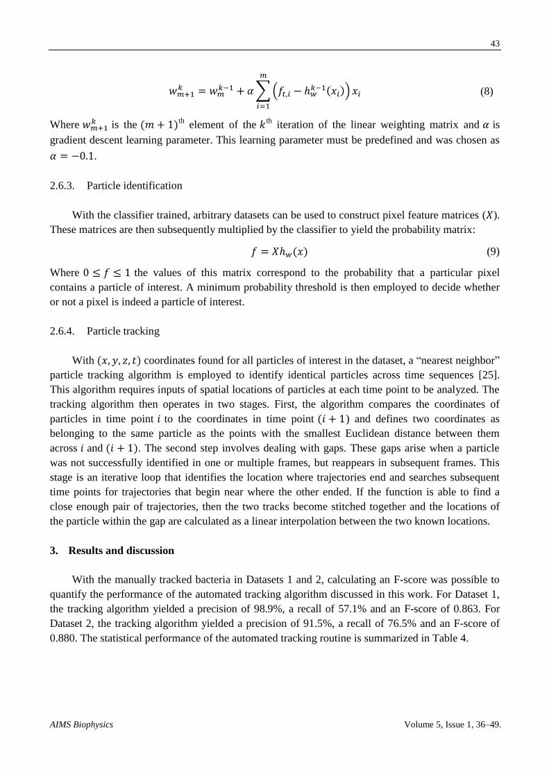
43

AIMS Biophysics Volume 5, Issue 1, 36–49.

∑(

)

(8)

Where is the th

element of the th iteration of the linear weighting matrix and is

gradient descent learning parameter. This learning parameter must be predefined and was chosen as

.

2.6.3. Particle identification

With the classifier trained, arbitrary datasets can be used to construct pixel feature matrices ( ).

These matrices are then subsequently multiplied by the classifier to yield the probability matrix:

(9)

Where the values of this matrix correspond to the probability that a particular pixel

contains a particle of interest. A minimum probability threshold is then employed to decide whether

or not a pixel is indeed a particle of interest.

2.6.4. Particle tracking

With coordinates found for all particles of interest in the dataset, a “nearest neighbor”

particle tracking algorithm is employed to identify identical particles across time sequences [25].

This algorithm requires inputs of spatial locations of particles at each time point to be analyzed. The

tracking algorithm then operates in two stages. First, the algorithm compares the coordinates of

particles in time point to the coordinates in time point ) and defines two coordinates as

belonging to the same particle as the points with the smallest Euclidean distance between them

across and . The second step involves dealing with gaps. These gaps arise when a particle

was not successfully identified in one or multiple frames, but reappears in subsequent frames. This

stage is an iterative loop that identifies the location where trajectories end and searches subsequent

time points for trajectories that begin near where the other ended. If the function is able to find a

close enough pair of trajectories, then the two tracks become stitched together and the locations of

the particle within the gap are calculated as a linear interpolation between the two known locations.

3. Results and discussion

With the manually tracked bacteria in Datasets 1 and 2, calculating an F-score was possible to

quantify the performance of the automated tracking algorithm discussed in this work. For Dataset 1,

the tracking algorithm yielded a precision of 98.9%, a recall of 57.1% and an F-score of 0.863. For

Dataset 2, the tracking algorithm yielded a precision of 91.5%, a recall of 76.5% and an F-score of

0.880. The statistical performance of the automated tracking routine is summarized in Table 4.

44

AIMS Biophysics Volume 5, Issue 1, 36–49.

Table 4. Performance statistics of automated tracking algorithm.

Dataset 1 Dataset 2

Total number of points 324 98

Total number of points identified 187 82

True positives 185 75

False positives 2 7

False negatives 139 23

Precision 98.8% 91.5%

Recall 57.1% 76.5%

F-score 0.863 0.880

Of the bacteria that were identified in Datasets 1 and 2, the localization errors were quantified

as the absolute Euclidean distance between the coordinates found by the algorithm and the

coordinates obtained by manual tracking. The root-mean-squared (RMS) localization error of Dataset

1 was found to be 7 µm and 6 µm for Dataset 2. Figure 1 shows the histogram of localization errors

from (a) Dataset 1 and (b) Dataset 2.

Figure 1. Localization error of the automated tracking algorithm of (a) Dataset 1 and (b)

Dataset 2.

The tracking algorithm was also employed to track a dataset with a higher concentration of

Bacillus subtilis (on the order of 106 cells per mL). At such a concentration, there are expected to be

a range of 100 to 200 cells in the field of view of the DHM instrument at any one time. The tracking

algorithm was able to identify 149 unique bacteria in this dataset, while a human observer was only

able to identify 127 bacteria. The remaining 22 bacteria were noticed by the human observer only

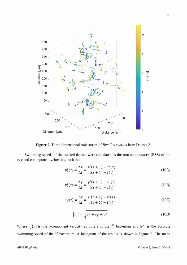
after they knew there were bacteria there. Figure 2 shows a three-dimensional plot of the trajectories

extracted from the tracking algorithm of this dense sample. The trajectories are color coded with

respect to time.

(a) (b)

45

AIMS Biophysics Volume 5, Issue 1, 36–49.

Figure 2. Three-dimensional trajectories of Bacillus subtilis from Dataset 3.

Swimming speeds of the tracked dataset were calculated as the root-sum-squared (RSS) of the

and component velocities, such that:

(10A)

(10B)

(10C)

| | √

(10D)

Where is the -component velocity at time of the th

bacterium and is the absolute

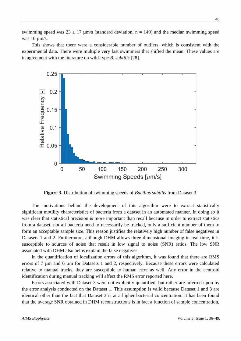
swimming speed of the th bacterium. A histogram of the results is shown in Figure 3. The mean

46

AIMS Biophysics Volume 5, Issue 1, 36–49.

swimming speed was 23 ± 17 µm/s (standard deviation, n = 149) and the median swimming speed

was 10 µm/s.

This shows that there were a considerable number of outliers, which is consistent with the

experimental data. There were multiple very fast swimmers that shifted the mean. These values are

in agreement with the literature on wild-type B. subtilis [28].

Figure 3. Distribution of swimming speeds of Bacillus subtilis from Dataset 3.

The motivations behind the development of this algorithm were to extract statistically

significant motility characteristics of bacteria from a dataset in an automated manner. In doing so it

was clear that statistical precision is more important than recall because in order to extract statistics

from a dataset, not all bacteria need to necessarily be tracked, only a sufficient number of them to

form an acceptable sample size. This reason justifies the relatively high number of false negatives in

Datasets 1 and 2. Furthermore, although DHM allows three-dimensional imaging in real-time, it is

susceptible to sources of noise that result in low signal to noise (SNR) ratios. The low SNR

associated with DHM also helps explain the false negatives.

In the quantification of localization errors of this algorithm, it was found that there are RMS

errors of 7 µm and 6 µm for Datasets 1 and 2, respectively. Because these errors were calculated

relative to manual tracks, they are susceptible to human error as well. Any error in the centroid

identification during manual tracking will affect the RMS error reported here.

Errors associated with Dataset 3 were not explicitly quantified, but rather are inferred upon by

the error analysis conducted on the Dataset 1. This assumption is valid because Dataset 1 and 3 are

identical other than the fact that Dataset 3 is at a higher bacterial concentration. It has been found

that the average SNR obtained in DHM reconstructions is in fact a function of sample concentration,

47

AIMS Biophysics Volume 5, Issue 1, 36–49.

but the degradation of SNR from the concentration of Dataset 1 to Dataset 3 was found to be

negligible [29].

A large hindrance of three-dimensional particle tracking is the data volumes associated with it.

In the particular setup used in this work, 4 megapixel holograms (roughly 4 MB per hologram) were

acquired at roughly 10 frames per second. Each hologram was then reconstructed into about 200

separate focal planes in both amplitude and phase. This results in a 400× increase in data size after

numerical reconstruction (e.g. Dataset 3 was over 100 GB in size). Non-trivial software techniques

must be employed in order to be able to analyze this volume of data with a modest computer. The

algorithm described in this work employs these techniques in order to only occupy 8 GB of RAM at

any one given time throughout the tracking process.

4. Conclusions

This work presents and validates a machine-learning identification algorithm based on linear

logistic regressions that can identify microorganisms within DHM image reconstructions, with a

precision of over 90% and localization error of roughly 7 µm. Identification was validated using

two species of microorganisms of different sizes, without the use of any chemical contrast

enhancement (e.g. fluorescent dyes).

The theoretical and mathematical foundation of this algorithm was introduced and discussed as

well as the method in which it was implemented as a MATLAB routine.

A total of three datasets were analyzed using this algorithm consisting of Bacillus subtilis and

Colwellia psychrerythraea. Two of the three datasets contained low concentrations of bacteria in

order to allow for the quantization of error, while the third dataset contained a much higher

concentration to illustrate its usefulness in practical biological imaging applications.

Although the data sizes associated with high spatial and temporal resolution three dimensional

imaging are cumbersome, the algorithm developed in this work is able to track particles in arbitrarily

large datasets (>100 GB) while only occupying 8 GB of RAM and modest CPU requirements. A

fully annotated version of the software developed and used throughout this work is available for

public use at: https://github.com/mbedross/MachineLearningObjectTracking.

Acknowledgments

The authors would like to acknowledge the Gordon and Betty Moore Foundation Grant

Numbers 4037/4038 as the source of funding for this work, as well as the Keck Center at Caltech for

hosting our collaborations.

Conflict of interest

The authors declare no conflicts of interest in this paper.

References

1. Taute KM, Gude S, Tans SJ, et al. (2015) High-throughput 3D tracking of bacteria on a standard

phase contrast microscope. Nat Commun 6: 8776.

48

AIMS Biophysics Volume 5, Issue 1, 36–49.

2. Molaei M, Barry M, Stocker R, et al. (2014) Failed escape: Solid surfaces prevent tumbling of

Escherichia coli. Phys Rev Lett 113: 068103.

3. Stocker R (2011) Reverse and flick: Hybrid locomotion in bacteria. Proc Natl Acad Sci USA

108: 2635–2636.

4. Schnars U, Jüptner W (1994) Direct recording of holograms by a CCD target and numerical

reconstruction. Appl Optics 33: 179–181. 5. Cuche E, Bevilacqua F, Depeursinge C (1999) Digital holography for quantitative phase-

contrast imaging. Opt Lett 24: 291–293. 6. Kühn J, Niraula B, Liewer K, et al. (2014) A Mach-Zender digital holographic microscope with

sub-micrometer resolution for imaging and tracking of marine micro-organisms. Rev Sci

Instrum 85: 123113. 7. Lee KR, Kim K, Jung J, et al. (2013) Quantitative phase imaging techniques for the study of cell

pathophysiology: From principles to applications. Sensors 13: 4170–4191. 8. Kim T, Zhou R, Mir M, et al. (2014) White-light diffraction tomography of unlabelled live cells.

Nat Photonics 8: 256–263.

9. Chengala A, Hondzo M, Sheng J (2013) Microalga propels along vorticity direction in a shear

flow. Phys Rev E 87: 052704. 10. Sheng J, Malkiel E, Katz J, et al. (2007) Digital holographic microscopy reveals prey-induced

changes in swimming behavior of predatory dinoflagellates. Proc Natl Acad Sci USA 104:

17512–17517. 11. Sheng J, Malkiel E, Katz J, et al. (2010) A dinoflagellate exploits toxins to immobilize prey

prior to ingestion. Proc Natl Acad Sci USA 107: 2082–2087. 12. Vater SM, Finlay J, Callow ME, et al. (2015) Holographic microscopy provides new insights

into the settlement of zoospores of the green alga Ulva linza on cationic oligopeptide surfaces.

Biofouling 31: 229–239. 13. Liu PY, Chin LK, Ser W, et al. (2016) Cell refractive index for cell biology and disease

diagnosis: Past, present and future. Lab Chip 16: 634–644. 14. Wallace JK, Rider S, Serabyn E, et al. (2015) Robust, compact implementation of an off-axis

digital holographic microscope. Opt Express 23: 17367–17378. 15. Molaei M, Sheng J (2014) Imaging bacterial 3D motion using digital in-line holographic

microscopy and correlation-based de-noising algorithm. Opt express 22: 32119–32137. 16. Bishara W, Sikora U, Mudanyali O, et al. (2011) Holographic pixel super-resolution in portable

lensless on-chip microscopy using a fiber-optic array. Lab Chip 11: 1276–1279. 17. Chengala A, Hondzo M, Sheng J (2013) Microalga propels along vorticity direction in a shear

flow. Phys Rev E 87: 052704. 18. Phan AH, Park JH, Kim N (2011) Super-Resolution Digital Holographic Microscopy for three

dimensional sample using multipoint light source illumination. Jpn J Appl Phys 50: 092503–092504. 19. Yuan C, Situ G, Pedrini G, et al. (2011) Resolution improvement in digital holography by

angular and polarization multiplexing. Appl Optics 50: B6–B11. 20. Rappaz B, Marquet P, Cuche E, et al. (2005) Measurement of the integral refractive index and

dynamic cell morphometry of living cells with digital holographic microscopy. Opt Express 13:

9361–9373. 21. Balaev AE, Dvoretski KN, Doubrovski VA (2002) Refractive index of escherichia coli cells.

Proc SPIE 4707: 253–260.

49

AIMS Biophysics Volume 5, Issue 1, 36–49.

22. Chenouard N, Smal I, Chaumont FD, et al. (2014) Objective comparison of particle tracking

methods. Nat Methods 11: 281–289. 23. Hosmer Jr DW, Lemeshow S (2004) Applied logistic regression. John Wiley Sons. 24. Junge K, Eicken H, Deming JW (2003) Motility of Colwellia psychrerythraea strain 34H at

subzero temperatures. Appl Environ Microbiol 69: 4282–4284. 25. Tinevez JY, Cao Y (2016) Simple Tracker. MATLAB Cent File Exc.

26. LynceeTec. Koala acquisition & analysis. Available from: http://www.lynceetec.com/koala-acquisition-

analysis/. 27. Schindelin J, Argandacarreras I, Frise E, et al. (2012) Fiji: An open-source platform for

biological-image analysis. Nat Methods 9: 676–682. 28. Ito M, Terahara N, Fujinami S, et al. (2005) Properties of motility in Bacillus subtilis powered

by the H+-coupled MotAB flagellar stator, Na

+-coupled MotPS or hybrid stators MotAS or

MotPB. J Mol Biol 352: 396–408. 29. Bedrossian M, Lindensmith C, Nadeau JL (2011) Digital holographic microscopy, a method for

detection of microorganisms in plume samples from Enceladus and other icy worlds.

Astrobiology 17: 913–925.

© 2018 the Author(s), licensee AIMS Press. This is an open access

article distributed under the terms of the Creative Commons

Attribution License (http://creativecommons.org/licenses/by/4.0)