A M AX IUENTR OPY METHOD F R S B NETWORK R G … · 1 A M AX IUENTR OPY METHOD F R S B NETWORK R G...

1 A MAXIMUM ENTROPY METHOD FOR SUBNETWORK ORIGIN-DESTINATION

2 TRIP MATRIX ESTIMATION

3

4 Chi Xie

5 Research Fellow

6 Department of Civil, Architectural and Environmental Engineering

7 The University of Texas at Austin – 6.506 E. Cockrell Jr. Hall

8 Austin, TX 78712-1076

9 [email protected]

10 Phone: 512-471-4622 & FAX: 512-475-8744

11

12 Kara M. Kockelman

13 (Corresponding author)

14 Professor and William J. Murray Jr. Fellow



17 Austin, TX 78712-1076

18 [email protected]

19 Phone: 512-471-0210 & FAX: 512-475-8744

20

21 S. Travis Waller

22 Associate Professor and Clyde E. Lee Fellow



25 Austin, TX 78712-1076

26 [email protected]

27 Phone: 512-471-4539 & FAX: 512-475-8744

28

29

30 The following paper is a pre-print and the final publication can be found in

31 Transportation Research Record No. 2196: 111-119, 2010.

32 Presented at the 89th Annual Meeting of the Transportation Research Board, January 2010

33

34

35 Key Words: Trip table estimation, subnetwork analysis, maximum entropy, linearization

36 algorithm, column generation

37

mailto:[email protected]



C. Xie, K.M. Kockelman and S.T. Waller 2

ABSTRACT 1

In the context of sketch planning, it is expected that a simplified network (i.e., an abstracted 2

network or subnetwork) model can accurately approximate the travel demand patterns and level-3

of-service attributes obtained from its full-network counterpart. A data prerequisite in this 4

approximation process is the trip matrix of the simplified network. This paper discusses a 5

maximum entropy method for the subnetwork trip matrix estimation problem, relying only on 6

link flow rates (estimated via full-network traffic assignment or as observed link-level vehicle 7

counts). A linearization algorithm of the Frank-Wolfe type is devised for problem solutions, in 8

which a column generation approach is iteratively used to solve the linearized subproblem 9

without path enumeration. Encouraging results from a numerical example suggest that this 10

method holds much promise for generating trip matrices that can be used to evaluate traffic flow 11

patterns under various network changes. 12

INTRODUCTION 13

Transportation planners almost always rely on simplified representations of roadway networks 14

for traffic analysis. For example, metropolitan areas often have networks with 10,000 of more 15

coded links, yet they ignore most local streets and they simplify intersection signal timing and 16

other details. In general, all models are abstractions of reality, and the level of details used 17

depends on desired accuracy in model outputs as well as available computational resources. 18

When the impacts of changes to a large network (such as that found in an urbanized area or 19

across a state) need to be anticipated, sketch planning is often considered as a cost-effective tool. 20

A sketch network may be a skeleton topology synthesizing only major arterials in the region (i.e., 21

an abstract network) or may focus on the details of a neighborhood or corridor of larger system 22

(i.e., a subnetwork). Such strategies are appealing when evaluation of the regional network 23

requires specialized expertise and/or is very computationally demanding, thus prohibiting 24

evaluation of one or more scenarios in a limited time frame. These simplified networks provide 25

planners with a less complex platform to facilitate quick-response and relatively informed 26

decision making early on. 27

While a number of studies addressed important theoretical and practical extraction/aggregation 28

issues for network abstraction (see 1-8), subnetwork analysis is still quite limited (see 9, 10). 29

Given a subnetwork extracted from a larger network, the first task we face is to determine the 30

subnetwork’s trip table. This is a data prerequisite for any subsequent travel demand analysis. 31

Specifically, this work’s objective is to derive a consistent origin-destination (O-D) trip matrix 32

for the subnetwork so that the travel demand analysis in the subnetwork (under changed network 33

conditions) will closely mimic full-network modeling results. 34


For a congested1 network experiencing user-equilibrium (UE) traffic conditions, one certainly 1

can estimate any subnetwork’s trip table by combining path flows from the full network, using a 2

procedure described by Haghani and Daskin (5, 6) and Hearn (11). This approach results in a 3

subnetwork trip matrix that can induce a link flow pattern in the subnetwork exactly as the same 4

as that in the larger system. However, this approach requires complete information on paths 5

taken in the full network and hence the resulting subnetwork trip matrix is dependent on the 6

given full-network path flow pattern. In general, unique path flow patterns do not exist in a UE 7

context, so this approach does not result in a unique subnetwork trip matrix. Thus, if such a 8

matrix were used to evaluate traffic shifts under network modifications (e.g., link additions 9

and/or expansion), the resulting flow estimates will likely deviate from full-network results. 10

Two complementary approaches may be used to eliminate this non-uniqueness issue, and both 11

make use of the entropy maximization principle (see 12, 13). The first approach is to estimate a 12

most likely, unique path flow pattern in the full network by means of an entropy-maximizing UE 13

traffic assignment algorithm (14-18) and then to aggregate corresponding path flows to form a 14

subnetwork trip matrix. The second approach requires only a link flow pattern from traffic 15

assignment in the full network; the link flows are used as inputs to a maximum entropy (ME) 16

method for estimating a most likely, unique O-D flow pattern for the subnetwork. 17

While one can debate which of the two procedures generates a more accurate and robust trip 18

matrix (in terms of the subnetwork evaluation result), we recommend the second approach, for 19

two computational and practical reasons. First, the second approach requires only link flow 20

information and conducts its ME optimization on the subnetwork level, which is much less 21

computationally demanding than the first approach (which conducts ME over the full network 22

and must store and manipulate path flows from the full network. The second reason relates to 23

the availability of input data. In cases where large-scale traffic assignment across the full 24

network is not feasible, one must rely on other data sources. Almost every traffic management 25

agency has a long history of collecting and assembling link-based traffic counts (e.g., for the 26

U.S.’s mandated Highway Performance Monitoring System [HPMS]). Thus, the second 27

approach is more practical in that it requires just subnetwork flow values, either estimated or 28

measured. For this reason, the second approach is the focus of this paper’s discussion. 29

The following section of this paper provide an overview of existing trip matrix estimation 30

methods, with a focus on traffic count-based methods. Next, a subnetwork matrix estimation 31

model based on ME theory is formulated and then analyzed, using a small numerical example for 32

interpreting the model’s optimality conditions. A linearization solution algorithm of the Frank-33

Wolfe type is devised for this convex optimization model, in each iteration of which the 34

linearized subproblem is solved by a column generation approach. (This avoids a reliance on 35

path enumeration.) The solution method is then applied to a small network with relatively large 36

1 The network does not really have to be congested, but the method applied here assumes that travel times are flow

dependent (so one cannot simply assume all-or-nothing assignments, for example).


network changes to assess their performance by comparing the traffic flow patterns generated by 1

the subnetwork and full-network traffic assignments. Finally, some modeling extensions are 2

suggested and research findings are summarized. 3

RELEVANT RESEARCH 4

Trip matrix estimation methods may be distinguished in terms of their theoretical basis (e.g., 5

gravity allocation, entropy maximization, and error minimization), traffic routing restrictions 6

(e.g., user equilibrium or proportional assignment), and required inputs (e.g., trip productions 7

and attractions, traffic counts, travel times, or target trip matrix). Count-based estimation 8

problems have been widely investigated and formulated in terms of a few different optimization 9

principles, including ME, least squares (LS), and maximum likelihood (ML), among others. 10

ME theory (or minimum information theory) was first used by Willumsen (19) and Van Zuylen 11

and Willumsen (20) for the most-likely-trip-matrix estimation problem, based on traffic counts. 12

By assuming that the underlying traffic flows follow a known proportional routing pattern, these 13

models resort to a simple iterative balancing method for solutions. In the same modeling 14

framework, Nguyen (21) formulated a ME problem synthesizing both traffic count data and trip 15

production and attraction data. While more information can be helpful, potential inconsistencies 16

across constraints can result in no feasible solutions. Fisk (22) imposed the UE routing principle 17

to a similar matrix estimation problem, resulting in a ME model subject to a variational 18

inequality constraint. His contribution is mostly theoretical, rather than practical, however; its 19

nonconvex feasible region makes the problem hard to solve. 20

Nguyen (23, 24) and others (24-27) pursued an alternative approach, incorporating equilibrium 21

traffic flows. Their approach uses minimum travel costs between all O-D pairs as inputs. 22

Knowing flows and link cost functions, link travel costs and path travel costs can be readily 23

calculated. The model makes no assumption about trip distribution patterns; however, 24

alternative optimal solutions may exist. To ensure convergence to a unique matrix solution, 25

some extra information (for example, a target trip matrix or the ME assumption) is generally 26

needed. 27

The joint use of (full or partial) traffic count and target matrix information has resulted in a 28

number of other trip matrix estimation methods, such as the Bayesian inference approach (28, 29

29), least squares approach (30-33), maximum likelihood approach (34-36, 29), constrained 30

regression approach (37), least absolute norm approach (38-40), and integrated squared error 31

approach (41). Despite various implicit parameter assumptions and optimization principles, all 32

seek a matrix that represents some form of trade-offs between a target trip matrix and observed 33

traffic counts. These trade-offs appear in the model constraints or objective functions. Due to 34

the above methods’ requirement of a target trip table, none applies here. 35


Given the fact that link flows (either estimates or measured counts) are the only data source 1

available in the context under study, we propose an ME model for subnetwork trip matrix 2

estimation. This approach is based on the early work of Willumsen (19) and Van Zuylen and 3

Willumsen (20). 4

MAXIMUM ENTROPY MODEL 5

Imagine a subnetwork , where and are the node and link sets of the subnetwork, 6

respectively. The origin node set and the destination node set are subsets of , (i.e., 7

and ). The proposed model implies two important assumptions, which greatly reduce the 8

modeling difficulty. (We later discuss how these assumptions can be removed, thereby 9

accommodating more general network conditions.) First, we assume that every node in the 10

network is potentially an origin and destination node (i.e., and ). If any node 11

cannot be an origin, one simply sets , ; similarly, if any node cannot be a 12

destination, one sets , . Second, we assume that the to-be-estimated subnetwork 13

trip matrix has fixed values. In other words, every O-D flow rate in the matrix is invariant to any 14

network change. In reality, all flows with external origin and/or external destination (i.e., outside 15

the subnetwork) can well change, as these tripmakers may seek different routes (potentially 16

avoiding the subnetwork entirely, or adding trips to the trip table). Thus, the greater the share of 17

trips involving origins or destinations outside the subnetwork, the more problematic is this 18

second assumption. 19

Nevertheless, given a complete set of estimated or measured link flow rates, , , one can 20

construct the following ME problem (P1): 21

max (1.1)

or min (1.2)

subject to (1.3)

, , (1.4)

where trip rate is defined as 22

, (1.5)


Here is the path flow rate of path between origin and destination . 1

This model’s functional form is common to the ME specifications used by Willumsen (19) and 2

Fisk (22). These models’ can all rely on link flow rates as the only input. (Production and 3

attraction data or some target O-D flow pattern is not required.) Note that the proposed 4

formulation (P1) does not imply any traffic routing assumption (i.e., how the estimated trip 5

matrix is assigned to generate the observed flow pattern in the network). In general, an 6

appropriate traffic routing principle needs to be specified and incorporated into the matrix 7

estimation process. For example, Willumsen’s ME model presumes that the proportions of any 8

O-D flow rate on traversed links are known a priori (so route choice is independent of 9

congestion), while Fisk’s model explicitly contains a UE traffic routing component. 10

In both Willumsen’s and Fisk’s models, observed link flows may contain noise and be 11

inconsistent with one another (e.g., flow may not be conserved at nodes); moreover, flow 12

observations are generally only available on a subset of network links. In the current context, by 13

contrast, a complete set of link flow rates is available, and the solution-implied flow rates may be 14

error-free, if these rates are produced by a traffic assignment process in the full network. Our 15

model does not require an explicit traffic assignment component, since the complete set of link 16

flows implies the desirable traffic flow pattern. If the given link flow pattern is achieved via a 17

UE traffic assignment in the full network, then the estimated subnetwork trip matrix can replicate 18

exactly the same flow pattern through a UE traffic assignment in the subnetwork. In fact, any 19

feasible solution of the ME model (P1) holds this conclusion, as proven here now. 20

Property 1. Assume that both the subnetwork and full-network traffic flow patterns are UE. A 21

subnetwork traffic assignment based on any feasible trip matrix solution of P1: 22

produces the same 23

subnetwork flow pattern (in terms of link flows) as the full-network traffic assignment. 24

Proof. Since the full-network flow pattern is UE, any part of the traffic flow pattern is UE. Let 25

us assume that a feasible trip matrix solution of P1 is obtained by decomposing into a 26

specific set of in terms of and then summing up this set of for 27

each O-D pair - , i.e., . 28

The UE traffic assignment problem for the subnetwork with this specific trip matrix is: 29

. It is 30

obvious that the specific path flow pattern and thus the link flow pattern 31

exactly satisfy the optimality condition of this traffic assignment problem. Because this traffic 32

assignment problem has a unique optimal solution (in terms of the link flow pattern), we know 33

that it is the link flow pattern . ∎ 34


Fortunately, this result does not mean that the proposed ME model will fail in the face of noisy 1

and inconsistent input data. Given the assumption that every node in the subnetwork can be an 2

origin and/or destination node, any set of flow rates can serve as an input data set. In other 3

words, an arbitrary set of input link flow rates contains some feasible solutions to the maximum 4

entropy model (P1). A more formal proof of this is as follows: 5

Property 2. Assume that every node in the network is potentially an origin and destination node. 6

Feasible solutions of P1 always exist given an arbitrary set of positive link flow rates. 7

Proof. The feasible solution set of P1 is confined by such a system of linear equations: 8

. Its feasibility is 9

equivalent to the feasibility of the reduced linear system of : 10

. Given that every , , , , exists, the 11

optimal solution of a quadratic program: 12

is , , where is a slack variable for link . The validity of this 13

least-squares method for checking the feasibility of linear systems can referenced in Carey and 14

Revelli (42). Thus, the existence of feasible solutions to P1 is guaranteed. ∎ 15

Note that, however, if the observed flow rates in the subnetwork are not UE (due to measurement 16

errors or other factors), the subnetwork trip matrix estimated from this disequilibrium flow 17

pattern will not result in the same flow pattern emerging from UE traffic assignment. The larger 18

the measurement errors are, the greater the deviation between the observed and produced traffic 19

flow patterns is. 20

In cases where traffic flow values on some links are missing, the model still produces a trip 21

matrix, except that those O-D flows using a path that fully consists of segments with missing 22

flow values will be underspecified. This is because path flows fully traversing segments with 23

missing data are unconstrained. 24

The optimality conditions of this subnetwork trip matrix estimation problem with an ―ideal‖ 25

input data set can be analyzed by using the Lagrangian of the model formulation, incorporating 26

the link flow conservation constraint: 27

(2)

where is the Lagrangian multiplier on link a’s flow-conservation constraint. Since the first-28

order condition of the Lagrangian with respect to path flow rate is: 29


(3)

the optimality conditions of the problem, and , can be 1

written as: 2

(4.1)

(4.2)

Note that denotes the minimum path ―entropy impedance‖ among all paths connecting 3

O-D pair . One can also define as the entropy impedance of link and define 4

as the entropy impedance of path between O-D pair , which is the sum of the 5

entropy impedances of all the links along this path. It becomes readily apparent that 6

, where link , if . Note that is the trip rate between O-D pair , 7

the head and tail nodes of link , which should not be confused with the link flow rate of link , 8

. Given these definitions, the optimality conditions of the defined ME problem can be stated 9

as follows. 10

Property 3. In an ME O-D flow pattern, all used paths (i.e., paths with a positive flow rate) 11

have their path entropy impedance equal to the minimum entropy impedance, and all unused 12

paths (i.e., paths with zero flow) are associated with a path entropy impedance greater than or 13

equal to the minimum impedance value. ∎ 14

This property describes the conditions of the path flow distribution in terms of entropy 15

impedance under the estimated ME O-D flows. Such an ME path flow pattern generally differs 16

from a UE path flow pattern derived in terms of travel cost, even if their corresponding link flow 17

patterns and O-D flow patterns are identical. More generally speaking, the path flow space 18

constrained by the ME O-D flow pattern (of the trip matrix problem) differs from the path flow 19

space constrained by the UE link flow pattern (of the traffic assignment problem). After all, the 20

trip matrix problem and the traffic assignment problem follow different optimality principles, 21

which result in different optimality conditions for path flows. 22

The solution uniqueness of the problem in terms of O-D flows is apparent thanks to the fact that 23

the objective function is strictly convex (i.e., its Hessian matrix is positive definite) and the 24

constraints (1.3)-(1.5) forms a convex feasible region. However, in general this ME problem 25

does not have a unique path flow solution. 26


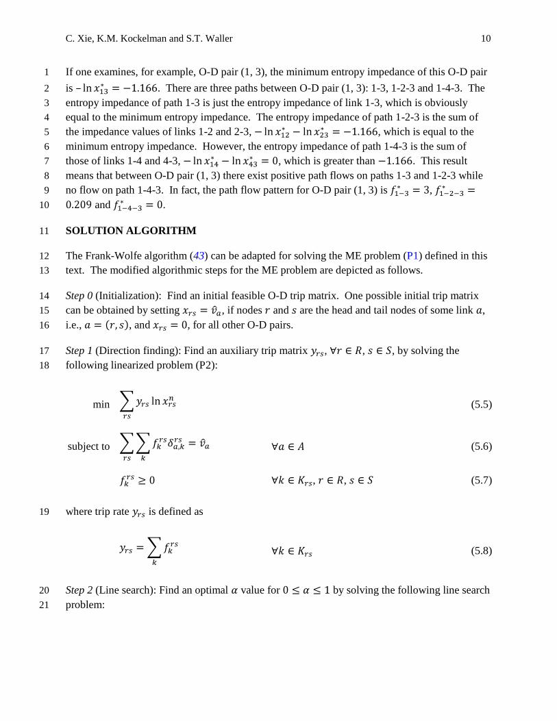
We use a toy network shown in Figure 1 to examine the optimal conditions of the ME problem 1

(P1). 2

Given five potential O-D pairs, (1, 2), (1, 3), (1, 4), (2, 3) and (4, 3), this ME problem is written 3

as follows: 4

min

where , , and , 5

subject to

, , , , , ,

where the O-D flow variables can be decomposed into path flow variables, 6

This numerical problem can be solved analytically as follows: Given , and 7

, one can reduce the objective function to 8

. This single-9

objective minimization problem can be readily solved by checking its partial gradient subject to 10

and , which results in and . Moreover, 11

, and as well. 12


If one examines, for example, O-D pair (1, 3), the minimum entropy impedance of this O-D pair 1

is – . There are three paths between O-D pair (1, 3): 1-3, 1-2-3 and 1-4-3. The 2

entropy impedance of path 1-3 is just the entropy impedance of link 1-3, which is obviously 3

equal to the minimum entropy impedance. The entropy impedance of path 1-2-3 is the sum of 4

the impedance values of links 1-2 and 2-3, , which is equal to the 5

minimum entropy impedance. However, the entropy impedance of path 1-4-3 is the sum of 6

those of links 1-4 and 4-3, , which is greater than . This result 7

means that between O-D pair (1, 3) there exist positive path flows on paths 1-3 and 1-2-3 while 8

no flow on path 1-4-3. In fact, the path flow pattern for O-D pair (1, 3) is , 9

and . 10

SOLUTION ALGORITHM 11

The Frank-Wolfe algorithm (43) can be adapted for solving the ME problem (P1) defined in this 12

text. The modified algorithmic steps for the ME problem are depicted as follows. 13

Step 0 (Initialization): Find an initial feasible O-D trip matrix. One possible initial trip matrix 14

can be obtained by setting , if nodes and are the head and tail nodes of some link , 15

i.e., , and , for all other O-D pairs. 16

Step 1 (Direction finding): Find an auxiliary trip matrix , , , by solving the 17

following linearized problem (P2): 18

min (5.5)

subject to (5.6)

, , (5.7)

where trip rate is defined as 19

(5.8)

Step 2 (Line search): Find an optimal value for by solving the following line search 20

problem: 21


min (6.1)

subject to (6.2)

Step 3 (Solution update): Set . 1

Step 4 (Convergence test): If a convergence criterion is met (for example, ), 2

stop; otherwise, go to step 1. 3

It should be noted that the computational bottleneck of the Frank-Wolfe algorithm in solving the 4

ME problem is the linearized ME subproblem formed in step 1. The standard linear 5

programming (LP) solution method — the simplex method — may not be directly applied to this 6

linear problem, because an explicit statement and processing of such an LP problem requires 7

enumeration of all possible path flows between each O-D pair, which is computationally 8

prohibitive for problems of realistic network size. For this reason, an efficient approach that 9

avoids path enumeration is required; otherwise, the application of the Frank-Wolfe algorithm for 10

the ME problem may be limited to subnetworks of small size only. 11

To relax the computational difficulty, this work resorts to the column generation approach, 12

which generates path flows only as and when needed within the solution framework of the 13

revised simplex method (see, e.g., 44 and 45). Given that the linearized problem is in the form 14

of path flows, we label the path set of the network as . Since the optimal 15

solution of this linearized problem is a basic feasible solution, it is readily known that there are at 16

most paths with positive flow rate in the optimal solution. 17

For convenience, one can first rewrite the linearized ME problem (P2) into the following path-18

based matrix form: 19

min (7.1)

where is the negative of the path entropy impedance vector, , and 20

is the path flow vector, , 21

subject to (7.2)

(7.3)

where is the link-path incidence matrix, , and is the estimated link flow 22

vector, . 23


Suppose that we are at some iteration of the simplex procedure, where the current basic feasible 1

solution contains basic paths of positive flow. The sets of basic paths and nonbasic paths are 2

labeled and , respectively. Suppose that the corresponding basis matrix and cost vector are 3

and , where and . Given the simplex multiplier vector 4

, one knows that the reduced cost for a nonbasic path flow variable is 5

, where is the corresponding column of to the nonbasic path . It 6

is readily known that if all reduced costs , , the current basic feasible 7

solution is optimal; otherwise, one may increase the path flow rate of a nonbasic path with 8

, from 0 to some positive level so that the objective function value is 9

decreased while the problem feasibility is maintained. In the latter case, a nonbasic path with the 10

lowest reduced cost value may be chosen for this purpose, according to Dantzig’s rule. Without 11

enumerating all the nonbasic paths in the set , Dantzig’s rule can be implemented by solving 12

the following minimization problem: 13

(8.1)

which can be further decomposed into a set of minimization problems by O-D pairs: 14

(8.2)

Note that the minimization problem for each O-D pair - is essentially a shortest path problem 15

(P4), as follows, given that is fixed for all paths between O-D pair - : 16

min (9.1)

subject to (9.2)

where is the link-path incidence vector of path between O-D pair - , which exists in as 17

a column. It is obvious that for this shortest path problem, the negative of the simplex multiplier 18

vector specifies the link costs over the network. It should be noted that an 19

arbitrary element in (or ) (i.e., the cost of an arbitrary link) may be positive or negative, so 20

a shortest path algorithm that prevents negative cost loops is needed. 21

After executing the shortest path search for each O-D pair, one can then obtain the entering path 22

flow variable (to the basis matrix) with the lowest value over all O-D pairs, which 23

generates a new column for the basis matrix, . The remaining algorithmic issue is to 24

determine the value of the entering path flow variable and accordingly identify a leaving path 25

flow variable (from the basis matrix). Suppose that the entering path is between O-D pair - 26


and its flow rate and the link-path incidence vector are and , respectively. Then the 1

leaving path flow variable is the one that maximizes the value while maintaining the 2

problem feasibility (i.e., all the basic feasible path flow variables must be greater than or equal to 3

0): 4

(10)

where is the vector of path flow variables corresponding to the current basis matrix and is 5

the link flow vector. Since (where each element in is equal to 1 or 0), the 6

inequality in (10) is reduced to , which in turn results in: 7

(11)

This result implies that should be set to equal the minimum link flow along path . 8

Accordingly, the path flow variables in the current basis matrix should be updated by 9

, in which the path flow variable whose value is decreased to 0 is the 10

leaving variable. 11

The algorithmic steps of the column generation approach described above can be summarized as 12

follows, which synthetically serve as step 1 of the Frank-Wolfe solution framework: 13

Step 1.1 (Initialization): Find an initial, feasible O-D trip matrix for the linearized problem. 14

Such an initial trip matrix can be obtained by setting for such a path between such an 15

O-D pair - that nodes and are the head and tail nodes of some link (i.e., ) and 16

path contains link only ( i.e., ) and , , and by setting , 17

between O-D pair - . The values of all other path flow variables are set to be 0. 18

Step 1.2 (Entering path choosing): Solve a shortest path problem defined in (9) for each O-D pair 19

and identify entering path flow variable with the minimum value over all O-D 20

pairs. If the minimum value is greater than or equal to 0, the current basic feasible 21

solution is optimal; otherwise, go to step 1.3. 22

Step 1.3 (Leaving path choosing): Compute the value of the entering path flow variable by 23

and identify the leaving path flow variable whose value is 24

decreased to 0. 25

Step 1.4 (Basis matrix updating): Update the basic feasible path flow variables by 26

and update the basis matrix by inserting the entering path’s link-path incidence 27

vector and removing the leaving path’s link-path incidence vector. 28


NUMERICAL EVALUATION 1

In this section, the solution method’s performance is evaluated using a numerical example (the 2

Sioux Falls network). The full network has 24 nodes and 76 links, while the subnetwork 3

includes 12 nodes and 34 links (see Figure 2). The subnetwork approximately covers the 4

downtown area of the City of Sioux Falls. 5

UE traffic assignment over the full network was conducted to estimate a link flow pattern 6

(Figure 2), which was then used as input data set for the subnetwork trip matrix estimation model. 7

The Frank-Wolfe algorithm with column generation was then applied to generate an EM trip 8

matrix with 121 O-D pairs for the subnetwork. The estimation’s accuracy was then indirectly 9

assessed by applying the estimated subnetwork trip matrix to generate a traffic flow pattern and 10

comparing it to that generated by the full-network traffic assignment. 11

For evaluation purposes, a list of synthetic network upgrade scenarios was developed, including 12

both capacity expansion and link addition cases, as shown in Table 1. The flow pattern 13

comparison results for these upgrade scenarios are plotted in Figure 3. Two performance 14

measures are used here, to indicate the difference between the full-network and subnetwork flow 15

patterns: -squared value ( ) from linear regression (of full-network flows following network 16

change on subnet estimates) and root mean square error (RMSE). Among these various 17

scenarios, values range from 0.963 to 0.993, indicating a very close match between the full-18

network and subnetwork link flow patterns. Similarly, the RMSE values always like below 10%, 19

across all scenarios, implying high accuracy in subnetwork assignment results. These results 20

allow us to conclude that such a subnetwork model serves as a good approximation to its 21

corresponding full-network model for sketch planning purposes. 22

It should be noted that the numerical experiment involves rather significant network upgrades, 23

effectively representing what is likely to serve as ―worst-case‖ situations, in terms of model 24

performance. In networks of larger or more realistic size, or where upgrades represent less of 25

change, one can expect that flow estimates will lie even closer to their full-network counterparts, 26

on average, since the impacts of network upgrades will diminish in relation to the larger, 27

relatively stable, network topology. 28

MODELING EXTENSIONS 29

There are important modeling possibilities that relax the two demand generation assumptions 30

embedded in the proposed ME model. These are restriction-free demand generation and the 31

invariant-demand trip matrix. 32

Recall that the first assumption allows any link flow errors or imbalances and inconsistencies to 33

be absorbed by relevant O-D pairs without affecting the problem’s solution feasibility and 34

estimation efficiency. However, in a realistic network, some ―intermediate‖ nodes cannot be 35


either an origin or destination node (e.g., the point of an off-ramp from a freeway link). If one 1

adds this restriction to the model, it may result in intermediate nodes where in-flow total does not 2

match out-flow, thus not satisfying the flow conservation principle. One can use to denote the 3

set of such intermediate nodes, where , and . The following, 4

enhanced subnetwork trip matrix model (P3) can accommodate this data inconsistency issue 5

while guaranteeing solution feasibility: 6

min (12.1)

subject to (12.2)

, , (12.3)

, (12.4)

where is defined as 7

, (12.5)

(12.6)

(12.7)

In this enhanced model, the added non-negative artificial variables and represent on link 8

the difference between link a’s input flows and its estimated link flow, consistent with the 9

estimated trip matrix. The error-minimizing term added into the weighted objective function, 10

, seeks to steer the estimated link flow pattern as close as possible to the 11

given link flow pattern, in the form of least squares. Here, is a weighting coefficient that 12

indicates the relative preference for or strength of the error-minimizing term to the entropy-13

maximizing term. 14

Relaxation of the second assumption (that trip tables are fixed) adds an extra modeling 15

dimension—trip generation—into the subnetwork trip matrix estimation problem, which favors a 16

more general demand modeling condition. Without loss of generality, one can categorize 17

subnetwork trips into four groups, in terms of their departure and arrival locations: 1) internal-18


internal flows; 2) internal-external flows; 3) external-internal flows; and 4) external-internal 1

flows. Assuming that the O-D trip matrix in the full network is known and fixed, we know that 2

the internal-internal O-D flow rates are also known and the trip production rates of all internal-3

external O-D pairs and the trip attraction rates of all external-internal pairs are known. The 4

remaining tasks are how to distribute the internal-external O-D flows to their origins, distribute 5

the external-internal O-D flows to their destinations, and distribute the external-external between 6

their candidate origins and destinations, where the origins of external-internal O-D flows, the 7

destinations of internal-external O-D flows and the origins and destinations of external-external 8

O-D flows are the trip entry and egress points to the subnetwork. 9

In view of such an O-D flow structure embedded within a subnetwork, we propose a combined 10

trip distribution and traffic assignment model, of which the trip distribution is still based on the 11

ME theory and the traffic assignment follows the UE principle. Given the input data sets (i.e., 12

internal-internal O-D flow rate , , , internal-external production rate , 13

, external-internal attraction rate , , and maximum external-external O-D 14

flow rate , , , where and are the internal origin and destination node 15

sets, and and are the external origin and destination node sets, respectively), the combined 16

model (P4) is given as follows: 17

min

(13.1)

subject to , (13.2)

(13.3)

(13.4)

, (13.5)


, , , , (13.6)

where O-D flow rates , , and , and link flow rate are defined as, 1

, (13.7)

(13.8)

(13.9)

(13.10)

(13.11)

Note that , , , , and are decision variables of the model, 2

among which represents the amount of external-external flows that choose not going 3

through the subnetwork. Moreover, it is assumed that link cost is a convex, increasing 4

function of link flow rate , and synthetic external-external O-D cost is also a convex, 5

increasing function of the relevant congestion level outside the subnetwork affecting the route 6

choice of potential travelers choosing a path between nodes and . 7

The validity of these two models can be readily proven by applying standard convex analysis 8

techniques. Due to space limitations, detailed analyses are omitted here. However, it is worth 9

mentioning here that the increasing complexity of the model’s structure can still be 10

accommodated by existing solution methods: the enhanced trip matrix estimation problem (P3) 11

can be solved by a similar procedure to the linearization algorithm (43) presented in this text, 12

while the elastic-demand trip matrix estimation problem (P4) can be solved by the partial 13

linearization algorithm (46). 14

CONCLUSIONS AND FURTHER WORK 15

In the domain of sketch planning, a network abstraction (or subtraction) process should satisfy 16

two criteria: 1) the simplified network should be small enough (in terms of the network size) so 17

that it can be managed and processed efficiently; 2) the simplified network should preserve 18

important network characteristics and behaviors so that the impacts of any network change can 19


be properly reflected. Here, the focus is on developing a subnetwork trip matrix that provides 1

link flows consistent with flow observations (from field surveys) or flow estimates (generated by 2

a full-network model). 3

Here, an ME model was suggested for subnetwork trip matrix estimation and a solution method 4

based on the Frank-Wolfe algorithm was devised. The adapted Frank-Wolfe algorithm requires 5

efficient solution of a linearized ME problem in each of its iterations. We proposed a column 6

generation approach that relaxes the minimum reduced cost search during the course of solving 7

the linearized problem to a set of shortest path problems, thus avoiding a computationally 8

prohibitive path enumeration process. The modeling philosophy and solution performance are 9

illustrated via a numerical example, under multiple network modification scenarios, the results of 10

which support the validity and accuracy of our subnetwork modeling methodology for sketch 11

planning. 12

The basic model and enhancements discussed here are likely to prove useful to much larger scale 13

tests, offering an opportunity for thoughtful, real-time network evaluations. Such tools should 14

prove helpful not only for quickly evaluating a variety of network improvement projects, but also 15

work zone constraints, operations policies, evacuation procedures, and other instances of 16

network changes, potentially in a real-time setting. 17

ACKNOWLEDGEMENTS 18

The authors are grateful for funding support from the Texas Department of Transportation, under 19

Research Project No. 0-6235 (titled ―Sketch Planning Techniques to Assess Regional Air Quality 20

Impacts of Congestion Mitigation Strategies‖). They also appreciate the use of Professor Hillel 21

Bar-Gera’s origin-based computer code for all traffic assignment results in the paper. 22

23

24

25

26

27

28

29

30

31


REFERENCES 1

[1] Chan, Y. A Method to Simplify Network Representation in Transportation Planning. 2

Transportation Research, Vol. 10, No. 3, 1976, pp. 179-191. 3

[2] Chan, Y., T.S. Shen, and N.M. Mahaba. Transportation Network Design Problem: 4

Application of a Hierarchical Search Algorithm. In Transportation Research Record: Journal of 5

Transportation Research Board, No. 1251, 1989, pp. 24-34. 6

[3] Eash, R.W., K.S. Chon, Y.J. Lee, and D.E. Boyce. Equilibrium Traffic Assignment on an 7

Aggregated Highway Network for Sketch Planning. In Transportation Research Record: Journal 8

of Transportation Research Board, No. 944, 1983, pp. 30-37. 9

[4] Kaplan, M.P., Y.J. Gur, and A.D. Vyas. Sketch Planning Model for Urban Transportation 10

Policy Analysis. In Transportation Research Record: Journal of Transportation Research Board, 11

No. 952, 1984, pp. 32-39. 12

[5] Haghani, A.E., and M.S. Daskin. Network Design Application of an Exaction Algorithm for 13

Network Aggregation. In Transportation Research Record: Journal of Transportation Research 14

Board, No. 944, 1984, pp. 37-46. 15

[6] Haghani, A.E., and M.S. Daskin. Aggregation Effects on the Network Design Problem. 16

Journal of Advanced Transportation, Vol. 20, No. 3, 1986, pp. 239-258. 17

[7] Taylor, M.A.P., W. Young, and P.W. Newton. PC-Based Sketch Planning Methods for 18

Transport and Urban Applications. Transportation, Vol. 14, No. 4, 1988, pp. 361-375. 19

[8] Rogus, M.J. Building Sketch Networks: The Development of Sketch Zones Boundaries and 20

Aggregation Process of Detailed Highway Networks. Working Paper No. 96-11, Chicago Area 21

Transportation Study, Chicago, IL, 1996. 22

[9] Dowling, R.G., and A.D. May. Comparison of Small-Area O-D Estimation Techniques. In 23

Transportation Research Record: Journal of Transportation Research Board, No. 1045, 1985, 24

pp. 9-15. 25

[10] Zhou, X., S. Erdogan, and H.S. Mahmassani. Dynamic Origin-Destination Trip Demand 26

Estimation for Subarea Analysis. In Transportation Research Record: Journal of Transportation 27

Research Board, No. 1964, 2006, pp. 176-184. 28

[11] Hearn, D.W. Practical and Theoretical Aspects of Aggregation Problems in Transportation 29

Planning Methods. Transportation Planning Models, M. Florian, Eds., North-Holland, 30

Amsterdam, The Netherlands, 1984, pp. 257-287. 31


[12] Wilson, A.G. Entropy in Urban and Regional Modeling. Pion, London, England, 1970. 1

[13] Oppenheim, N. Urban Travel Demand Modeling: From Individual Choices to General 2

Equilibrium. Wiley, New York, NY, 1995. 3

[14] Rossi, T.F., S. McNeil, and C. Hendrickson. Entropy Model for Consistent Impact-Fee 4

Assessment. Journal of Urban Planning and Development, Vol. 115, No. 2, 1989, pp. 51-63. 5

[15] Bell, M.G.H., and Y. Iida. Transportation Network Analysis. Wiley, New York, NY, 1997. 6

[16] Janson, B.N. Most Likely Origin-Destination Link Uses from Equilibrium Assignment. 7

Transportation Research, Vol. 27B, No. 5, 1993, pp. 333-350. 8

[17] Larsson, T., J.T., Lundgren, C. Rydergren, and M. Patriksson. Most Likely Traffic 9

Equilibrium Route Flows Analysis and Computation. Equilibrium Problems: Nonsmooth 10

Optimization and Variational Inequality Models, F. Giannessi Eds., Springer, New York, NY, 11

2002, pp. 129-159. 12

[18] Bar-Gera, H. Primal Method for Determining the Most Likely Route Flows in Large Road 13

Networks. Transportation Science, Vol. 40, No. 3, 2006, pp. 269-286. 14

[19] Willumsen, L.G. Simplified Transport Models Based on Traffic Counts. Transportation, 15

Vol. 10, No. 3, 1981, pp. 257-278. 16

[20] Van Zuylen, H.J., and L.G. Willumsen. The Most Likely Trip Matrix Estimated from 17

Traffic Counts. Transportation Research, Vol. 14B, No. 3, 1980, pp. 281-293. 18

[21] Nguyen, S. Modèles de Distribution Spatial Tenant Compte des Itinéraries. Publication No. 19

225, Centre de Recherché sur les Transports, Univerité de Montréal, Montreal, Canada, 1981. 20

[22] Fisk, C.S. On Combining Maximum Entropy Trip Matrix Estimation with User Optimal 21

Assignment. Transportation Research, Vol. 22B, No. 1, 1988, pp. 69-79. 22

[23] Nguyen, S. Estimation an O-D Matrix from Network Data: A Network Equilibrium 23

Approach. Publication No. 60, Centre de Recherché sur les Transports, Université de Montréal, 24

Montreal, Canada, 1977. 25

[24] Nguyen, S. Estimating Origin-Destination Matrices from Observed Flows. Transportation 26

Planning Models, F. Florian Eds., Elsevier, Amsterdam, The Netherlands, 1984, pp. 363-380. 27

[25] Turnquist, M.A., and Y. Gur. Estimation of Trip Tables from Observed Link Volumes. In 28

Transportation Research Record: Journal of Transportation Research Board, No. 730, 1979, pp. 29

1-6. 30


[26] LeBlanc, L.J., and K. Farhangian. Selection of a Trip Table Which Reproduces Observed 1

Link Flows. Transportation Research, Vol. 16B, No. 2, 1982, pp. 83-88. 2

[27] Yang, H., Y. Iida, and T. Sasaki. The Equilibrium-Based Origin-Destination Matrix 3

Estimation Problem. Transportation Research, Vol. 28B, No. 1, 1994, pp. 23-33. 4

[28] Maher, N.J. Inferences on Trip Matrices from Observations on Link Volumes: A Bayesian 5

Statistical Approach. Transportation Research, Vol. 17B, No. 6, 1983, pp. 435-447. 6

[29] Lo, H.P., N. Zhang, and W.H.K. Lam. Estimation of an Origin-Destination Matrix with 7

Random Link Choice Proportions: A Statistical Approach. Transportation Research, Vol. 30B, 8

No. 4, 1996, pp. 309-324. 9

[30] Cascetta, E. Estimation of Trip Matrices from Traffic Counts and Survey Data: A 10

Generalized Least Square Estimator. Transportation Research, Vol. 18B, No. 4/5, 1984, pp. 289-11

299. 12

[31] Hendrickson, C., and S. McNeil. Matrix Entry Estimation Errors. Proceedings of the 9th 13

International Symposium on Transportation and Traffic Theory, Delft, The Netherlands, 1984, 14

pp. 413-430. 15

[32] Bell, M.G.H. The Estimation of an Origin-Destination Matrix from Traffic Counts. 16

Transportation Science, Vol. 17, No. 1, 1991, pp. 198-217. 17

[33] Yang, H., T., Sasaki, Y. Iida, and Y. Asakura. Estimation of Origin-Destination Matrices 18

from Link Traffic Counts on Congested Networks. Transportation Research, Vol. 26B, No. 6, 19

1992, pp. 417-434. 20

[34] Bell, M.G.H. The Estimation of an Origin-Destination Matrix from Traffic Counts. 21

Transportation Science, Vol. 17, No. 2, 1983, pp. 198-217. 22

[35] Bell, M.G.H. Variances and Covariances for Origin-Destination Flows When Estimated by 23

Log-Linear Models. Transportation Research, Vol. 19B, No. 6, 1985, pp. 497-507. 24

[36] Spiess, H. A Maximum Likelihood Model for Estimating Origin-Destination Matrices. 25

Transportation Research, Vol. 21B, No. 5, 1987, pp. 395-412. 26

[37] McNeil, S., and C. Hendrickson. A Regression Formulation of the Matrix Estimation 27

Problem. Transportation Science, Vol. 19, No. 3, 1985, pp. 278-292. 28

[38] Yang, H., Y. Iida, and T. Sasaki. An Analysis of the Reliability of an Origin-Destination 29

Trip Matrix Estimated from Traffic Counts. Transportation Research, Vol. 25B, No. 5, 1991, pp. 30

351-363. 31


[39] Sherali, H.D., R. Sivanandan, and A.G. Hobeika. A Linear Programming Approach for 1

Synthesizing Origin-Destination Trip Tables from Link Traffic Volumes. Transportation 2

Research, Vol. 28B, No. 3, 1994, pp. 213-233. 3

[40] Nie, Y., and D.H. Lee. Uncoupled Method for Equilibrium-Based Linear Path Flow 4

Estimator for Origin-Destination Trip Matrices. In Transportation Research Record: Journal of 5

Transportation Research Board, No. 1783, 2002, pp. 72-79. 6

[41] Gajewski, B.J., L.R., Rilett, M.P. Dixon, and C.H. Spiegelman. Robust Estimation of 7

Origin-Destination Matrices. Journal of Transportation and Statistics, Vol. 5, No. 2/3, 2002, pp. 8

37-56. 9

[42] Carey, M., and R. Revelli. Constrained Estimation of Direct Demand Functions snd Trip 10

Matrices. Transportation Science, Vol. 20, No. 3, 1986, pp. 143-152. 11

[43] Frank, M., and P. Wolfe. An Algorithm for Quadratic Programming. Naval Research 12

Logistics Quarterly, Vol. 3, No. 1-2, 1956, pp. 95-110. 13

[44] Dantzig, G.B. Linear Progrmming and Extensions. Princeton University Press, Princeton, 14

NJ, 1963. 15

[45] Bazaraa, M.S., J.J. Jarvis, and H.D. Sherali. Linear Programming and Network Flows. 16

Wiley, New York, NY, 1990. 17

[46] Evans, S. Derivation and Analysis of Some Models for Combining Trip Distribution and 18

Assignment. Transportation Research, Vol. 9, No. 12, 1976, pp. 241-246. 19


TABLE 1 List of Network Upgrading Scenarios

Scenario number Network upgrading location, type and scale

1 Increasing capacity by 50 percent on road segments 4-11-14

2 Increasing capacity by 50 percent on road segments 5-9-10-15

3 Increasing capacity by 50 percent on road segments 6-8-16-17-19




7 Increasing capacity by 50 percent on road segments 10-17

8 Adding two road segments 4-9 and 9-11

9 Adding a road segment 10-14

FIGURE 1 An Illustrative Example For The Maximum Entropy Problem

1

2

3

V23 = 2

V13 = 3

V12 = 2

4

V14 = 1 V43 = 1


FIGURE 2 The Sioux Falls Network and Its Subnetwork Traffic Flow Pattern

1 2

8806

8798

18031

18006

6883

6837

1112 1610

11073

11047

17727

17604

21

81

4

21

74

4

84

07

83

89

3 4

53

00

52

00

5

15

79

7

15

78

1

9

6

12

52

6

12

49

3

8

8100

8100

97

76

23

19

2

11

68

4

11

69

5

19117

19083

9080

9036

23 22

14 15

17

99

42

99

53

19

2413 2021

18

7

The subnetwork

98

14

23

12

6


(a) Scenario 1 (b) Scenario 2 (c) Scenario 3

(d) Scenario 4 (e) Scenario 5 (f) Scenario 6

(g) Scenario 7 (h) Scenario 8 (i) Scenario 9

FIGURE 3 Link Flow Rates Estimated Using Full-Network And Subnetwork Traffic

Assignments

R² = 0.9854

0

5000

10000

15000

20000

25000

30000

0 5000 10000 15000 20000 25000 30000

Fu

ll-n

etw

ork

lin

k flo

w r

ate

Subnetwork link flow rate

RMSE = 0.051R² = 0.9629

0

5000

10000

15000

20000

25000

30000

0 5000 10000 15000 20000 25000 30000

Fu

ll-n

etw

ork

lin

k flo

w r

ate


RMSE = 0.084

R² = 0.9924

0

5000

10000

15000

20000

25000

30000

0 5000 10000 15000 20000 25000 30000

Fu

ll-n

etw

ork

lin

k flo

w r

ate


RMSE = 0.038

R² = 0.9874

0

5000

10000

15000

20000

25000

30000

0 5000 10000 15000 20000 25000 30000

Fu

ll-n

etw

ork

lin

k flo

w r

ate


RMSE = 0.043 R² = 0.968

0

5000

10000

15000

20000

25000

30000

0 5000 10000 15000 20000 25000 30000

Fu

ll-n

etw

ork

lin

k flo

w r

ate


RMSE = 0.080

R² = 0.9679

0

5000

10000

15000

20000

25000

30000

0 5000 10000 15000 20000 25000 30000

Fu

ll-n

etw

ork

lin

k flo

w r

ate


RMSE = 0.065

R² = 0.9934

0

5000

10000

15000

20000

25000

30000

0 5000 10000 15000 20000 25000 30000

Fu

ll-n

etw

ork

lin

k flo

w r

ate


RMSE = 0.039

R² = 0.9859

0

5000

10000

15000

20000

25000

30000

0 5000 10000 15000 20000 25000 30000

Fu

ll-n

etw

ork

lin

k flo

w r

ate


RMSE = 0.086

R² = 0.9698

0

5000

10000

15000

20000

25000

30000

0 5000 10000 15000 20000 25000 30000

Fu

ll-n

etw

ork

lin

k flo

w r

ate


RMSE = 0.094

A M AX IUENTR OPY METHOD F R S B NETWORK R G … · 1 A M AX IUENTR OPY METHOD F R S B NETWORK R G...

Documents

Transcript of A M AX IUENTR OPY METHOD F R S B NETWORK R G … · 1 A M AX IUENTR OPY METHOD F R S B NETWORK R G...