A Low-Carbon Fuel Standard for California - California …€¦ · · 2007-08-012007-08-01 · A...
108
A Low-Carbon Fuel Standard for California Part 2: Policy Analysis August 1, 2007 Project Directors Alexander E. Farrell, UC Berkeley Daniel Sperling, UC Davis Contributors A.R. Brandt, A. Eggert, A.E. Farrell, B.K. Haya, J. Hughes, B.M. Jenkins, A.D. Jones, D.M. Kammen, C.R. Knittel, M.W. Melaina, M. O’Hare, R.J. Plevin, D. Sperling
Transcript of A Low-Carbon Fuel Standard for California - California …€¦ · · 2007-08-012007-08-01 · A...

A Low-Carbon Fuel Standard for California
Part 2: Policy Analysis
August 1, 2007
Project Directors Alexander E. Farrell, UC Berkeley
Daniel Sperling, UC Davis
Contributors A.R. Brandt, A. Eggert, A.E. Farrell, B.K. Haya, J. Hughes, B.M. Jenkins, A.D. Jones,
D.M. Kammen, C.R. Knittel, M.W. Melaina, M. O’Hare, R.J. Plevin, D. Sperling

A Low Carbon Fuel Standard for California Part II: Policy Analysis Page ii
(This page is intentionally blank.)

A Low Carbon Fuel Standard for California Part II: Policy Analysis Page iii
TABLE OF CONTENTS
List of Figures .................................................................................................................... iv List of Tables ..................................................................................................................... iv Acknowledgments .............................................................................................................. v Executive Summary ............................................................................................................ 1 1 Introduction .................................................................................................................. 7
1.1 Context ............................................................................................................... 8 1.2 Structure of the report......................................................................................... 8
2 Background .................................................................................................................. 9 2.1 Similar initiatives in the US and UK .................................................................. 9 2.2 Challenges of innovative policy ....................................................................... 13 2.3 Market failures and barriers as a basis for policy design.................................. 16 2.4 Competition among fuels.................................................................................. 22
3 Program Design.......................................................................................................... 25 3.1 Scope of the standard........................................................................................ 25 3.2 Diesel fuel......................................................................................................... 27 3.3 Baselines & targets ........................................................................................... 31 3.4 Point of regulation ............................................................................................ 36 3.5 Upstream emissions.......................................................................................... 41 3.6 A default and opt in system for the carbon intensity of fuels ........................... 44 3.7 Trading and banking of credits ......................................................................... 50 3.8 Compliance and penalties ................................................................................. 52 3.9 Certification/auditing processes........................................................................ 54
4 Measurement and certification ................................................................................... 57 4.1 Drivetrain efficiency adjustment factors .......................................................... 57 4.2 Offsets and opt-ins............................................................................................ 58 4.3 Carbon capture and storage .............................................................................. 59 4.4 Dealing with uncertainty in life cycle analyses ................................................ 61 4.5 Land use change ............................................................................................... 62
5 Related Issues ............................................................................................................. 69 5.1 Interactions with AB1493 (Pavley) GHG standards for vehicles..................... 69 5.2 Interactions with AB32 regulations .................................................................. 70 5.3 Interactions with other policy instruments and initiatives ................................ 71 5.4 Innovation credits ............................................................................................. 72 5.5 Environmental justice and sustainability issues ............................................... 75 5.6 Regulatory capacity needed by the state........................................................... 76 5.7 Program review................................................................................................. 77 5.8 Cost analysis ..................................................................................................... 78 5.9 Research needs ................................................................................................. 80
6 References .................................................................................................................. 83 Appendix A: VISION-CA scenarios with indirect land use change................................. 89 Appendix B: Structure of the California Oil, Electricity, and Natural Gas Industries...... 98 Appendix C: Simple Calculation of Indirect Land Use Change Effects......................... 102

A Low Carbon Fuel Standard for California Part II: Policy Analysis Page iv
List of Figures Figure 2-1: The eight modules used in the RTFO carbon calculation.......................................... 11 Figure 2-2: The RD3 innovation pipeline: research, development, demonstration and deployment (adapted from PCAST, 1999) ....................................................................................................... 14 Figure 3-1: Illustrative compliance paths for the LCFS ............................................................... 35 Figure 3-2: Illustrative example of the default and opt in system ................................................ 46 Figure 5-1: Carbon reduction credits and technology innovation credits as a function of carbon reductions relative to gasoline and fuel carbon intensity.............................................................. 73
List of Tables Table 2-1: Selected non-technical factors that will influence the competition among fuels ........ 23 Table 3-1: Principal California transportation fuels and uses....................................................... 25 Table 3-2: Illustrative LCFS compliance schedules ..................................................................... 35 Table 3-3: Hierarchy of Biofuel Default Values from the UK RTFO. (E4Tech 2007)................ 47 Table 3-4: Selected estimates of GHG emissions costs................................................................ 54 Table 4-1: Additional emissions associated with crop-based biofuel based on a simple approach attributing crop-related land use conversion effects to all cropland equally ................................ 65

A Low Carbon Fuel Standard for California Part II: Policy Analysis Page v
Acknowledgments This research was supported by the Energy Foundation. The authors would like to thank the staffs of the California Air Resources Board, California Energy Commission, California Public Utility Commission, and representatives of the many stakeholder organizations who participated in the study. The view and opinions herein, as well as any remaining errors, are those of the authors alone and do not necessarily represent the views of the sponsor or any other organization or person.
© Copyright Regents of the University of California

A Low Carbon Fuel Standard for California Part II: Policy Analysis Page 1
Executive Summary The Low Carbon Fuel Standard (LCFS) can play a major role in reducing greenhouse gas emissions and stimulating improvements in transportation fuel technologies so that California can meet its climate policy goals. In Part 1 of this study we evaluated the technical feasibility of achieving a 10 percent reduction in the carbon intensity (measured in gCO2e/MJ) of transportation fuels in California by 2020. We identified six scenarios based on a variety of different technologies that could meet or exceed this goal, and concluded that the goal was ambitious but attainable. In Part 2, we examine many of the specific policy issues needed to achieve this ambitious target. Our recommendations are based on the best information we were able to gather in the time available, including consultation with many different stakeholders. The recommendations are intended to assist the California Air Resources Board, Energy Commission, and Public Utility Commission, as well as private organizations and individuals, in addressing the many complex issues involved in designing a low carbon fuel standard. Choices about specific policies and calculation of numeric values for use in regulation must, of course, be made by these regulatory agencies. The analysis we present here is only illustrative. The need to significantly reduce greenhouse gas (GHG) emissions from the transportation sector opens up the possibility that new fuels and new vehicles may become economical and widely used. The introduction of new transportation fuels that do not require petroleum will have a co-benefit: reduced oil imports to the state and the nation. It is important to note that these new fuels will compete on a very uneven playing field: the size, organization, and regulation of these industries are radically different. It is unreasonable to think that these differences will be eliminated by the LCFS. The LCFS should be designed to reduce in the barriers and disincentives facing energy companies that might offer low carbon fuels to consumers. Technological innovation is crucial to the success of the LCFS and to the achievement of California’s climate change goals. At the same time, imposing a new regulatory requirement will cause markets to shift (or rationalize) their existing production and sales so that improvements appear on paper to have been made, when in reality no significant change has occurred. Obviously, this rationalization does not represent the type of innovation needed to support the state’s climate change goals. The implementation of the LCFS must recognize and manage both of these effects, rewarding innovation while also minimizing unproductive “rationaqlization.” For this reason, we suggest that the LCFS require modest reductions in carbon intensity in the early years, and steeper reductions later as innovations and new investments bring more low carbon transportation fuels to market. The LCFS should not be seen as a singular policy. It can provide complementary incentives to an economy-wide GHG emission cap, should the state choose to impose one. Implementing the LCFS requirement with a provision for trading and banking of credits will tend to keep costs low. And the LCFS should also be coordinated with other climate change policies. In addition, the LCFS may have implications for broader issues, such as environmental justice and sustainability, and should be implemented with these issues in mind. Considerable increases in the administrative capability of the regulating agencies will be needed in order to successfully implement the LCFS, and this capability should be assisted by continued research support.

A Low Carbon Fuel Standard for California Part II: Policy Analysis Page 2
One of the most challenging issues in the implementation of the LCFS is the climatic effect of land use change due to expansion of biofuel production. Because food and energy markets are global, all agricultural production contributes to the pressure to clear new land for crops. Recent scientific investigations suggest that enormous amounts of greenhouse gases can be released when lands are converted to more intensive cultivation (and also cause other adverse effects such as reduced biodiversity and changed water flows). These land use effects have been largely ignored in earlier lifecycle greenhouse gas assessments of biofuels. Because of these effects, all biofuels produced from crops grown on arable land face serious challenges if they are to be used to lower GHG emissions. If biofuels are to reduce greenhouse gas emissions relative to fossil-based gasoline and diesel, then biofuels must: i) use advanced production methods (some of which are available now), ii) be derived from feedstocks grown on degraded land, or iii) be produced from wastes or resides. Land use change effects should be included in the LCFS, though cautiously at first, with the understanding that further research may change our understanding of this issue and therefore how it should be regulated. The LCFS provides a durable framework for reducing the large amount of greenhouse gases, especially CO2, that are emitted from today’s petroleum-based transport fuel system. It will facilitate the introduction of low-carbon fuels and restrain the trend toward investments in more carbon intense transport fuels. These unconventional resources, including heavy oil, tar sands, oil shale and coal, have higher, sometimes much higher, carbon emissions than fuels made from conventional petroleum. The LCFS is a response to this recarbonization of transportation fuels, as well as the many market failures blocking innovation and investments in low-carbon alternatives to petroleum. We have the following specific recommendations: R1: Scope of the standard For liquid fuels, the LCFS should apply to all gasoline and diesel used in California for use in transportation, including freight and off-road applications. The LCFS should also allow providers of non-liquid fuels (electricity, natural gas, propane, and hydrogen) sold in California for use in transportation to participate in the LCFS or have the associated emissions covered by another regulatory program. If the number of non-liquid-fueled vehicles grows in the future, mandatory participation in the LCFS may need to be considered.
R2: Diesel fuel Differences in the drive train efficiencies of diesel and gasoline engines should be accounted for and heavy and light duty diesel fuels should be treated differently to prevent the possibility that unrelated increases in diesel consumption could lead to compliance without achieving the goals of the LCFS.
R3: Baseline & targets The baseline year should be the most recent year for which data are available before the LCFS was announced. A uniform state-wide baseline should be applied to all regulated entities. We recommend a compliance path that does not require significant near-term carbon intensity reductions, in order to allow technologies to develop. If implemented through a decline in carbon intensity, the ARB must evaluate the amount of shifting of production and sales (“rationalization”) that may occur. If implemented through a technology standard in the early

A Low Carbon Fuel Standard for California Part II: Policy Analysis Page 3
years, the ARB must evaluate what is an advanced biofuel and what is not. If rationalization can account for a large fraction of the 2020 goal, the target may need to be made more stringent to ensure the goals of the LCFS are met.
R4: Point of regulation The LCFS regulation should be imposed upon entities that produce or import transportation fuel for use in California. For liquid fuels, these are refiners, blenders and importers, and the point of regulation should be the point at which finished gasoline or diesel is first manufactured or imported. For electricity and gaseous fuel providers that choose to participate in the LCFS, the regulated entities should be distributors of the fuel and the point of regulation should be the supply of electricity or fuel to the vehicle.
R5: Upstream emissions GHG emissions from the production of fuels should be included in the LCFS.
R6: A default and opt in system for the carbon intensity of fuels To the degree possible, values used to certify the carbon intensity (i.e., GWI) of different fuels should be based upon empirical data representative of the specific inputs and processes in each fuel’s life cycle. Pessimistic default values should be determined by state agencies for each of these inputs and processes. Fuel providers will face the option of either adopting these pessimistic values (with GWI values higher than average values) or opting in by providing sufficient data to certify a lower life cycle GWI value for a particular fuel.
R7: Trading and banking of credits The ability of regulated firms to trade and bank credits is critical to the cost-effectiveness of the LCFS. There should be no limit on the ability of any legal entity to trade or bank (hold) LCFS credits. Compliance using banked LCFS credits is allowed with no discount or other adjustment. Borrowing should not be allowed.
R8: Compliance and penalties Obligated parties should have the option to comply with the LCFS by paying a fee, which is different from paying a fine for non-compliance. We discuss different approaches to setting the fee level. In addition, high penalties should be imposed for willfully misreporting data or other fraudulent acts.
R9: Certification/auditing processes Methods and protocols need to be established to verify that claimed credits are accurate. We recommend that third party auditors be used, financed through fees paid by those companies claiming credits beyond the default values.
R10: Drivetrain efficiency adjustment factors The carbon intensity metric for the LCFS should take into account the inherent efficiency differences with which different fuels are converted into motive power. The efficiency adjustment factors associated with different fuels should ideally reflect actual vehicles on the road, and be based upon empirical data. We discuss different approaches to developing and measuring these drivetrain efficiency adjustment factors.
R11: Offsets and opt-ins Offsets generated from within the transportation sector, such as “opt-in” reductions from marine or aviation transport, should be available as credits within the LCFS. Offsets from outside the transportation sector should not be allowed, at least in the initial years of the LCFS.

A Low Carbon Fuel Standard for California Part II: Policy Analysis Page 4
R12: Carbon capture and storage If carbon capture and storage (CCS) technologies that are safe and adequately monitored are developed, CCS projects directly related to the supply of transportation energy should be included within the LCFS. However, CCS activities outside of the transportation sector should not count toward LCFS targets.
R13: Dealing with uncertainty in life cycle analysis Life cycle analysis methods are an appropriate quantitative framework for the LCFS. Existing data are of sufficient quality to use life cycle methods in LCFS implementation, but a program to improve these methods should be implemented as well.
R14: Land use change Develop a non-zero estimate of the global warming impact of direct and indirect land use change for crop-based biofuels, and use this value for the first several years of the LCFS implementation. Participate in the development of an internationally accepted methodology for accounting for land use change, and adopt this methodology following an appropriate review.
R15: Interactions with AB1493 (Pavley) GHG standards for vehicles Keep LCFS and AB 1493 separate initially but consider integration at a later date.
R16: Interactions with AB32 regulations The design of both the LCFS and AB32 polices must be coordinated and it is not possible to specify one without the other. However, it is clear that if the AB32 program includes a hard cap, the intensity-based LCFS must be separate or the cap will be meaningless. Including the transport sector in both the AB32 regulatory program and LCFS will provide complementary incentives and is feasible.
R17: Interactions with other policy instruments and initiatives The LCFS will likely interact with many other government policies and initiatives, but a complete search for such interactions was not feasible here. More research is needed.
R18: Innovation credits Assigning additional credits for more innovative low carbon fuels should be considered.
R19: Environmental justice and sustainability issues Fuel providers should be required to report on the sustainability impacts of their fuels, especially those related to biofuels. The state should perform a periodic assessment of the impacts of the LCFS, in California, the US and globally, and should consider policies and sustainability metrics to mitigate these effects as we learn about them. Biofuels produced on protected lands should be excluded from the LCFS. The ARB should conduct more research on sustainability impacts, paying close attention to international efforts. At the start of LCFS implementation, we recommend against regulatory requirements beyond the reporting and land exclusion provisions. At the mid-course review, the effectiveness of the reporting requirements should be evaluated and the adoption of additional sustainability metrics should be considered.
R20: Program review Conduct a 5 year review, beginning in 2013, of data, methods, fuel production technologies, and advanced vehicle technologies. The intent is not to review the intensity targets, unless climate science has so radically changed that we are much more confident than today that either greater or lesser reductions are required.

A Low Carbon Fuel Standard for California Part II: Policy Analysis Page 5
R21: Cost analysis The ARB should conduct a cost analysis of the LCFS following the cost-effectiveness approach used in evaluating the U.S. Clean Air Act. This analysis should acknowledge uncertainties due to proprietary information and innovation in low-carbon energy technologies. It should also include a discussion of non-climate related costs and benefits.
R22: Research needs A great deal of research is needed to successfully implement the LCFS. Key areas include better characterization of the global warming impacts of different fuels, tools to allow regulators and obligated parties to assess different fuel production pathways, uncertainties in these values, the role of land use, environmental justice and sustainability goals, and the GHG implications of the vehicle lifecycle.

A Low Carbon Fuel Standard for California Part II: Policy Analysis Page 6
(This page is intentionally blank.)

A Low Carbon Fuel Standard for California Part II: Policy Analysis Page 7
1 Introduction This report examines the implementation of a Low Carbon Fuel Standard (LCFS) for California. This program will reduce the global warming effect of vehicle fuels used in the state over the decade beginning in 2010 and will begin the process of technological innovation to help stabilize the climate system (in conjunction with other policies). In Part 1 of this study, which examined a wide range of vehicle fuel options, we found a 10 percent reduction in the carbon intensity of transportation fuels by 2020 to be ambitious but attainable. In this Part 2 report, we examine the design of the LCFS and recommend actions to implement it. These suggestions and recommendations will be taken into consideration by the California Air Resources Board, California Public Utilities Commission, and California Energy Commission in their rulemaking processes. Under the LCFS, fuel providers would be required to track the life cycle global warming intensity (GWI) of their products, measured on a per-unit-energy basis, and reduce this value over time. The term life cycle refers to all activities included in the production, transport, storage and use of the fuel. A more complete analysis would also include energy embodied in the materials used in all these activities through their own production, such as batteries in electric vehicles, tractors used for cultivating the biofuel crops, and oil refinery equipment. In practice, taking the analysis to this more complete accounting would be very difficult, and in most cases it probably would not substantially change the relative emissions ratings of the different fuel paths.1 Future improvements in methods used for the LCFS might include a more complete materials analysis, but for now a more limited approach is adequate. The term global warming intensity is a measure of all of the mechanisms that affect global climate, including not only greenhouse gases (GHGs) but also other processes. For instance, conversion of land use to produce biomass feedstocks can change albedo and evapotranspiration, both potentially important effects on climate change (Gibbard, 2005; Marland, 2003). However, it is not clear at this time how to measure these effects in the context of the LCFS and their inclusion may need to be left to the future. Land use change effects are likely to increase the GWI of some biofuels, but not biofuels made from wastes or residues. Thus, uncertainty in future GHG emission estimates from biofuel production due to land use change apply to current biofuels that are made from feedstocks grown on fertile soil and possibly biofuels made from feedstocks grown on degraded land. The unit of measure for GWI used in this study is grams of carbon dioxide equivalent per megajoule used to propel a vehicle (gCO2e/MJ). It is calculated by adjusting the gCO2e/MJ of fuel entering the vehicle for inherent differences in the in-use energy efficiency of different fuels (e.g., diesel, electricity and hydrogen) (see Part 1 section 2.3). For convenience, the term carbon intensity is used to refer to the total life cycle GWI per unit of fuel energy delivered to do useful work at the wheel of a vehicle. The goal of the LCFS is to reduce the average fuel carbon
1 Possible exceptions include vehicles that use fuel cells or large storage batteries, which may have significantly
different energy and material requirements in their production or disposal. Evaluating these effects and what the correct role (if any) in regulating them is an important research task.

A Low Carbon Fuel Standard for California Part II: Policy Analysis Page 8
intensity (AFCI) for all transportation fuels used in the state of California, measured in units of (adjusted) gCO2e/MJ. The findings and recommendations contained in this report are the result of extensive consultation with representatives of oil companies, electric and natural gas utilities, biofuel companies, environmental groups, CARB, and CEC, as well as with others from the PUC and car companies. This report benefited from that extensive input, but it is a policy analysis and not a political weighing of interests and values. Our recommendations are directed at the public interest, broadly conceived, and is designed to inform and facilitate an administrative/political decision process to follow. In the end, though, the findings and recommendations, as well as any errors, are those of the authors alone and do not necessarily represent the views of the sponsor, CARB, CEC, or any other organization or person.
1.1 Context
The larger context of the climate policy into which the LCFS is set is described in the Introduction to Part 1 of this study. The goals of California climate policy are to:
1. Encourage investment and improvement in current and near-term technologies that will help meet the 2020 target,
2. Stimulate innovation and development of new technologies that can dramatically lower GHG emissions at low costs and can start to be deployed by 2020 or soon thereafter, creating the conditions for meeting the later 2050 goal,
3. Contribute to attainment of related objectives as much as possible, including economic growth, air quality, other environmental protection goals, affordable energy prices, environmental justice, and diverse and reliable energy sources.
Accomplishing these three goals will help slow and eventually arrest global warming caused by increasing levels of GHGs in the earth’s atmosphere, both by reducing the emission of these gases in California and by setting an example for other jurisdictions – state, national, and international – to consider. A wide range of policies for addressing climate change have been identified (Alic 1999), and significant work has been done to articulate policy options specific to the transportation sector (Bandivadekar and Heywood 2004, Greene et al. 2005). Three fundamental strategies may be pursued to reduce GHG emissions in the transportation sector: improve vehicle technologies, reduce GHGs associated with fuels, and reduce vehicle travel. This report and this LCFS policy both are targeted at fuels. All three strategies will likely be necessary to achieve transportation’s share of the state’s 2020 statutory GHG emission targets (to reduce economy-wide emissions back to 1990 levels by 2020), and all three will definitely be necessary to achieve the goal of 80 percent reduction by 2050.
1.2 Structure of the report
This report has six sections, including this introduction. Section two provides background on policy issues and relevant experiences elsewhere. Section three describes the main program

A Low Carbon Fuel Standard for California Part II: Policy Analysis Page 9
design elements necessary to implement the LCFS. Section four addresses measurement and certification issues, and section five addresses a number of important related policy questions. Recommendations are highlighted in each of these sections. References make up the final section. Three appendices are also included.
2 Background
2.1 Similar initiatives in the US and UK
Other jurisdictions, notably in Europe, are beginning to provide examples of how the carbon intensity of fuels can be regulated. California can learn and expand upon these other efforts. Indeed, the proposed design of California’s LCFS discussed below borrows from efforts elsewhere, especially in the United Kingdom. And the recommended LCFS design for California is premised on being consistent and eventually integrated with initiatives elsewhere. Below, we examine a renewable fuel program being implemented in the United Kingdom that includes GHG emission tracking beginning in this year, and rules recently finalized by the U.S. Environmental Protection Agency (EPA) to implement the Renewable Fuel Standard (RFS).
2.1.1 UK Renewable Transport Fuel Obligation The UK Renewable Transport Fuel Obligation Programme2 (RTFO) requires fossil transport fuel suppliers, as of April 2008, to ensure that biofuels constitute 2.5% of total road transport fuels in 2008-09, 3.75% in 2009-10, and 5% in 2010-11 and beyond (Department for Transport 2006). Draft RTFO legislation was released in February 2007 for a consultation period lasting into May. The RTFO is expected to enter into force in April 2008. The RTFO was developed in cooperation with a large number of stakeholders through the Low Carbon Vehicle Partnership and represents a practical approach to managing the carbon intensity of vehicle fuels.3 The main objective of the RTFO is to reduce GHG emissions from the transport sector, while avoiding unintended negative impacts associated with biofuels, including environmental and social effects often called “sustainability impacts” (Department for Transport 2006). To meet these goals, the RTFO includes reporting requirements and methodologies for calculating life cycle GHG emissions as well as social and environmental sustainability aspects of individual biofuel pathways. The GHG and sustainability metrics will not initially be used in the calculations of compliance credits, however. The reporting requirement allows the regulators to determine the feasibility, accuracy, and efficiency of such reporting and to provide industry with some experience prior to linking these metrics to the incentive structure. We recommend a similar reporting requirement for the California LCFS in section 3.5. According to the Consultation on the Draft RTFO Order (similar to a Regulatory Impact Analysis), “The [UK] Government is committed to promoting the use of only the most sustainable biofuels with a low carbon intensity towards meeting the RTFO. The Government is keen to move as soon as possible to a system under which only those biofuels which can be proved to come from sustainable sources are eligible for renewable transport fuel certificates
2 The official website for the RTFO is http://www.dft.gov.uk/roads/RTFO 3 See http://www.lowcvp.org.uk/

A Low Carbon Fuel Standard for California Part II: Policy Analysis Page 10
under the RTFO, and under which different biofuels are rewarded according to the level of carbon savings that they offer” (Department for Transport 2006). Another important consideration—especially in the UK, which imports most of its biofuels—is the legality under international trade rules of banning certain biofuels or feedstocks. Bans that are strictly aligned with policy objectives, e.g., the reduction of GHG emissions, are considered more likely to survive challenges in the World Trade Organization (WTO). According to the consultants developing the carbon reporting standard, the German government may soon test this principle by implementing a ban on certain biofuels (Watson 2007). This is relevant for the LCFS because imports of biofuels might be a strategy for some regulated entities, although this compliance strategy was not evaluated in Part 1 of this study due to data limitations. The RTFO recognizes that in the short term, the primary strategy for reducing the GHG impact of transportation fuels is to blend petroleum fuels with low-GHG biofuels. Unlike California’s LCFS, the UK regulation does not cover gaseous fuels or electricity as transportation fuels (although biogas is eligible for credits). In our view, apart from the more limited approach, the RTFO represents a well-designed policy approach that can and should be adapted to the LCFS. Below is a summary of elements of the RTFO that have inspired some of our recommendations for the LCFS.
2.1.1.1 Renewable transport fuel certificates The RTFO includes a certificate trading scheme in which fossil-based transport fuel suppliers can meet their renewable fuel requirement by any combination of (a) selling renewable transport fuel, for which they receive certificates, (b) purchasing certificates from another company, or (c) paying a “buy-out” price per unit of renewable fuel that the company should have supplied, but did not. For 2008/09, the buy-out price has been set at 15 pence per liter ($1.10/gal)4. The buy-out fees will contribute to a fund that is disbursed at the end of each compliance period to all entities that have submitted certificates to the RTFO administrator as evidence of having sold the corresponding quantity of renewable fuel, in proportion with the number of certificates submitted. This payout from the fund provides additional incentives to supply biofuels.
2.1.1.2 Default values and carbon accounting methodology The two main goals of the carbon accounting methodology are (1) to encourage and facilitate accurate reporting of actual fuel chains in use, and (2) to be easy to use, yet capable of handling the GHG emissions from a wide range of biofuel pathways (Bauen, Watson, and Howes 2006). Regulated companies will report on the carbon savings delivered by their renewable transport fuels, based on a defined calculation methodology. The methodology defines a series of modules that compute the carbon intensity of each step in the biofuels production chain, as depicted in Figure 2-1.
4 Currency conversion on 1-16-07 using rate of 1 GBP = 1.96 USD.

A Low Carbon Fuel Standard for California Part II: Policy Analysis Page 11
Figure 2-1: The eight modules used in the RTFO carbon calculation The methodology allows producers to accept default values for their fuel’s GHG intensity, but these values are intentionally set high to encourage companies to provide more accurate, process-specific data. (Some default values are set as typical depending on their use, e.g. when they represent a relatively minor part of the energy usage.) The methodology also includes default values for individual parameters (e.g., to compute the GHG intensity of feedstocks used) to allow carbon savings to be estimated where figures are not available. Default values are determined by panels of experts and maintained by the RTFO Administrator. (Additional details of the RTFO methodology are discussed in section 2.1 of this report, as our recommendations are informed significantly by this work.)
2.1.1.3 Carbon accounting tool The carbon accounting methodology software to be developed will be essential for both compliance and for producers to explore the ramifications of potential changes to their production methods. The tool will provide a simple interface allowing users to choose default values or enter specific data to compute the carbon intensity of the various components of the product chain (Bauen, Howes, and Franzosi 2006). Users include feedstock producers or collectors, intermediaries (e.g., transport companies), and biorefineries. Each category of user will need to provide data for a different set of modules. At each stage, users require the ability to input and aggregate the results of prior stages to compute their total GWI of the production chain through their portion of the process. The tool will produce data files that can be communicated across the production chain with the feedstock or fuel, allowing downstream entities to correctly account for upstream emissions.
2.1.1.4 Biofuels sustainability reporting Regulated companies must also report on the broader environmental and social sustainability of their renewable fuels. The methodology for this is still under development. These requirements will apply to both UK-produced and imported biofuels.

A Low Carbon Fuel Standard for California Part II: Policy Analysis Page 12
2.1.1.5 Implications of the RTFO for the LCFS While the RTFO involves only biofuels, the basic approach can be readily expanded to incorporate all fuels regulated under the LCFS, although applying this method to petroleum fuels may be challenging. For a fuller elaboration of the RTFO approach and methods, see (Bauen, Watson, and Howes 2006; Bauen, Howes, and Franzosi 2006).
2.1.2 U.S. Renewable Fuel Standard (RFS) The other initiative that is most relevant to the LCFS is EPA’s recently established Renewable Fuels Standard (RFS) program, mandated by the Energy Policy Act of 2005. This program is designed to ensure that a minimum volume of “renewable fuels” is blended into US motor vehicle fuels. The final rules were published in May 2007 (EPA 2007) and enter into force October 1, 2007. Interim rules apply for the months leading up to October 2007. The final rules establish specific targets for renewable fuel volumes, a market-based compliance credit trading scheme, and equivalency factors for different fuels such as corn ethanol, cellulosic ethanol, and biodiesel. The renewable volume targets specified in the Energy Policy Act of 2005 begin with 4 billion gallons in 2006, increasing to 7.5 billion gallons in 2012. EPA is required to establish targets for 2013 and beyond based on a review of the first 6 years of the program. These targets have not yet been set, but President Bush has proposed a future goal of 35 billion gallons of “alternative” fuels by 2017, which is defined to include not just renewable fuels, but also other alternatives such as coal-to-liquids. (An important distinction between the national EPA and California LCFS programs is that the LCFS program is premised on a carbon metric, while the national program has no environmental metric associated with it. This distinction is important since greenhouse gas emissions from alternative fuels can exceed that of conventional gasoline, depending on the production process. In the proposed new federal “alternative fuel” program, the use of liquids made from coal could cause increases in GHG emissions from transportation.) The overall goal of the current RFS is to encourage the use of renewable fuels, which are defined broadly as any motor vehicle fuel produced from plant or animal products or wastes, as opposed to being produced from fossil fuels. Each renewable fuel is assigned an equivalency value based on the energetic content of the fuel relative to denatured ethanol. Thus denatured starch-based ethanol is assigned an equivalency value of 1, whereas FAME biodiesel is assigned an equivalency value of 1.5 because it is more energy dense. For fuels made from both renewable and fossil based feedstocks, the energetic proportion of renewable content in the final fuel determines the equivalency value. The Energy Policy Act of 2005 mandates that cellulosic ethanol be credited 2.5 times the value of starch-based ethanol, despite equal energetic content in the fuels. This multiplier is intended to incentivize investments in cellulosic biofuels, because the production potential is greater and the environmental impacts less. As a mechanism to credit more environmentally beneficial fuels, this is a rather ad-hoc measure compared to the life cycle assessment approach called for by the LCFS. The RFS rules require each batch of renewable fuels to be assigned a unique Renewable Identification Number (RIN). This number accompanies the fuel until it is blended into a finished transportation fuel. At this point, the RIN can be separated from the fuel and sold in an open market to regulated entities, which must acquire a set number of RIN equivalents each

A Low Carbon Fuel Standard for California Part II: Policy Analysis Page 13
calendar year in order to demonstrate compliance with the RFS. The equivalency value discussed above is encoded in the RIN, thus some RINs count further toward compliance than others.
2.1.2.1 Environmental Information in the RFS Program The RINs do not include environmental information at this time, but they could in the future. EPA considered two methods of incorporating environmental information about different fuels into the RFS. One method consisted of assigning equivalency values to fuels based on life cycle analyses of the energetic inputs or greenhouse-gas emissions associated with fuel production, rather than simply the energy contained in the final fuel. This method would have been similar to the LCFS. The second method was a voluntary environmental rating that could be incorporated into the RIN number. EPA ultimately rejected both but has recently indicated that it is willing to work with stakeholders to re-consider the use of environmental information in RINs.
2.1.2.2 Implications of the RFS for the LCFS Inclusion of life cycle GWI information in the RIN would be very helpful as long as the life cycle methodology used is consistent with the goals of the LCFS. This is true regardless of where in the distribution cycle the fuel is regulated, because the environmental information in RINs will remain attached to the fuels until they are blended into finished fuels. Trading of RINs may create some accounting challenges because entities regulated under the RFS can purchase RINs for fuels that they have not themselves blended, including fuels blended outside the state of California. If environmental information in RINs is used to support the LCFS, then only RINs which are still associated with their original fuel should be considered. The entities which separate RINs under the RFS may or may not be those that are obligated to meet the LCFS requirement. One way to incorporate environmental information in the RIN into the LCFS would be to permit entities who separate RINs from fuels to generate LCFS paperwork that remains attached to the fuel once RINs are sold.
2.2 Challenges of innovative policy
A wide range of studies have recognized the essential role of technology innovation as a basis for economic growth and efficiency. The process of technology innovation is complex and multifaceted, and varies significantly among sectors. A study of innovation in the energy sector by the President’s Council of Advisors on Science and Technology (PCAST, 1999) used a linear model to describe the different activities associated with the innovation process. As shown in Figure 2-1, this linear model portrays innovation as a series of sequential phases linking the results from basic R&D to commercialization. This “RD3 innovation pipeline” begins with invention and discovery in the research and development phase, followed by production increase in the demonstration phase, cost reductions with increased production in the learning and buydown phase (Wene, 2000), and finally widespread deployment in the final commercialization phase. Though this linear model is a simplification of a much more complex process, it is useful for identifying and articulating the types of policies that can target specific activities within the innovation process. The LCFS serves as a “demand pull” policy for technologies that have advanced to or beyond the demonstration phase within the RD3 innovation pipeline, as distinguished from “supply push” policies, like subsidies for particular production practices or products. This policy influence has

A Low Carbon Fuel Standard for California Part II: Policy Analysis Page 14
the potential to fulfill the first climate change policy goal stated in the introduction, where technologically proven or off-the-shelf technologies are deployed to meet the near-term 2020 intensity target. The second climate change policy goal, stimulating the development of new low carbon fuels that will be sufficient to meet California’s long-term 2050 climate stabilization target, will require advances in technologies that have yet to reach or move beyond the demonstration phase. The LCFS will not necessarily provide sufficient support for advances at this level of innovation; additional targeted policies may be required to assure the success of these long-term and low carbon technologies. Similarly, and perhaps more importantly, the LCFS also does not necessarily provide sufficient support for advanced vehicle technologies that will likely be required for the success of some vehicle-fuel combinations, such as battery electric vehicles (BEVs) and hydrogen fuel cell vehicles (HFCVs).
Research & Development
Demonstration & Increase in Scale
Learning & Buydown
Widespread Deployment
Scale
TimeSmall
Medium
Commercial
$/unit
Cumulative Production
Figure 2-2: The RD3 innovation pipeline: research, development, demonstration and deployment (adapted from PCAST, 1999) There are two possible pathways through which the LCFS can induce innovation. In the first, the LCFS would reduce the carbon intensity of existing fuels and close substitutes, requiring little change in vehicle technology. In the second more challenging path, the LCFS would induce a shift toward different vehicle technologies such as electric-drive and fuel cells, and dedicated non-petroleum vehicles. The second innovation pathway requires actions beyond the capacity of any single economic decision-maker. It requires investments and decisions by a variety of fuel suppliers and distributors, vehicle manufacturers, and consumers. Typically, fuels are not substitutable in the short run. A driver of a gasoline vehicle can't use diesel or electricity regardless of price. Vehicles capable of using the lower-GWI fuel must be built, consumers must purchase them, and fueling infrastructure must be provided (such as E85 filling stations, dedicated vehicle charging stations and meters in residences, and hydrogen infrastructure). The LCFS acts directly on the parties most involved in the first pathway and only indirectly on the key decision-makers involved in the second, especially vehicle makers and vehicle consumers. Short of a dramatic tightening of the LCFS beyond 2020, the LCFS, by itself, may be insufficient to bring about the second pathway. The case of bi-fueled vehicles like plug-in hybrid electric vehicles (PHEVs) is somewhat different. They have the advantage of running on multiple fuels, and are less dependent upon a pervasive alternative fuel infrastructure. PHEVs do not face the infrastructure challenges of

A Low Carbon Fuel Standard for California Part II: Policy Analysis Page 15
hydrogen or other types of dedicated vehicles due to the widespread availability of electricity. However, some infrastructure is likely to be needed, even for PHEVs, and especially if the electricity they use is to be differentiated from other types of electricity (say, with a special rate). In this case a dedicated meter and plug are likely to be needed – which might be feasible in most suburban homes, but less so in many urbanized locations. Fuel flexibility may come at a higher vehicle cost (as in the case of PHEVs) or it may reduce other vehicle attributes (such as size or interior space). The deployment of bi-fueled and flex-fueled vehicles may be an important part of the development of low-carbon fuels, but the long-term viability of some low carbon fuels may be dependent on the widespread success of dedicated alternative fuel vehicles that have been optimized for a particular fuel. The structural attributes of the vehicle-fuel systems discussed above exemplify specific limitations of a market mechanism like the LCFS to promote innovation, and will probably result in stronger incentives for clean fuels that require little change to the vehicle fleet and much weaker incentives for fuels that also require vehicle switching. While the LCFS can be used to send signals toward low carbon fuels, this signal is stronger for liquid fuels that power conventional engines than for other alternative fuels. Additional incentives will probably be needed to support markets for fuels that require dedicated vehicles. The scenarios discussed in Part 1 of this study begin to explore some of these issues and illuminate the large number of changes that may need to take place for the LCFS to be met. For example, electric and CNG vehicles might need to be produced and offered for sale, ethanol and/or biodiesel may need to be manufactured differently and possibly in increased quantity, fuel distributors would need to buy these products and prepare appropriate blends. Farmers would need to plant and harvest feedstocks (possibly new feedstocks), and solid waste handlers, including governments, would need to extract cellulosic materials from waste streams. Some new technologies may need to be developed and commercialized to meet even the 2020 reduction target. And regulators need to develop rules and certification programs that will guide these activities. Most firms will tend to respond to the LCFS in a manner that relies upon their existing technological and organizational areas of expertise. In some cases, firms may branch out to acquire additional expertise in areas specific to a particular low carbon fuel. For example, most petroleum refiners do not currently have expertise with animal oil and fat markets, municipal solid waste streams or land management practices. Acquiring expertise in these types of areas might require significant human and capital resources, and significant effort would be necessary to reach the level of learning attained by other firms with a history in these areas. These investments in new expertise will most likely be decided strategically, and will likely be viewed in terms of long-term payoffs resulting from technological advantage in future low carbon fuel markets (BCG 1968). It is unlikely that these innovation investment decisions would be made only to comply with the LCFS in the near-term. Despite the many opportunities to invest in new areas of expertise, compliance with the LCFS in the near term will be achieved by either purchasing credits from other low carbon fuel producers or by relying upon existing technological expertise. Purchasing credits allows a regulated entity

A Low Carbon Fuel Standard for California Part II: Policy Analysis Page 16
to comply with the LCFS without making the high-risk or long-term commitments needed to attain additional expertise in novel or unfamiliar low carbon fuel technologies. And by selling credits, low carbon fuel producing firms receive additional revenue to help recoup investments made in innovation and learning. This transfer can, in theory, reinforce the expertise acquired by firms that are most successful in producing low carbon fuels. This can lead to increased learning (while partially offsetting R&D losses from spillover effects), resulting ultimately in reduced costs for some low carbon fuels. Whether the key developments are the product of small operators who sell their inventions to large companies, or the R&D efforts of the current dominant players in the vehicle fuel market, remains to be seen. It bears emphasis that the industrial organization of low-carbon transportation is not predictable at present even though plausible scenarios can be sketched; our recommendations lean heavily on allowing the maximum scope for innovation and market-guided evolution.
2.3 Market failures and barriers as a basis for policy design
Policy intervention in the energy sector has a long history. It has historically reflected both actions to direct energy firms to better serve the public interest (environmental controls on extraction and refining, antitrust actions against oil monopolies, pollutant regulations) and actions to favor parts of the industry (depletion tax credits). The motivation for global warming policy is a broadly accepted recognition that the market by itself will not achieve a socially optimal level of GHG emissions, one much lower than presently observed and very much lower than reasonably foreseeable in coming decades. As was the case for the regulatory approaches employed when earlier energy types were introduced (i.e., coal, oil, natural gas, nuclear, etc.), the approach taken for low carbon transportation fuels will reflect the political climate and regulatory paradigms that dominate policy processes at the time that they are introduced (Davis, 1993). The range of possible policy instruments to reduce GHGs in the transport sector range from pure market instruments, such as the carbon tax, to prescriptive regulatory instruments. Less straightforward market instruments include fees and rebates on vehicle purchase based on GHG emissions. Even more mixed approaches include caps on emissions with provisions for trading and banking. They also include intensity and performance targets, again with provisions with trading and banking. All of these approaches have pros and cons. The LCFS is a hybrid of market and regulatory approaches, and therefore combines aspects of two contemporary regulatory paradigms. It is regulatory in the sense that an intensity target is assigned to energy providers in one sector. And it is market-based in that energy providers can trade credits with each other (and possibly with others in the future). The LCFS, implemented properly, provides a framework for near-term reductions in emissions and also motivates a process of technological innovation necessary (but not sufficient) to meet long-term climate stabilization goals. The next section reviews different market failures and barriers associated with low carbon fuels. In many instances, these market failures and barriers are similar to those found to limit investments in energy efficiency technologies and other low-carbon energy production technologies (Brown 2001, Norberg-Bohm 2002). Our goal here is to highlight some of the major issues that should be taken into account in designing a LCFS. Market failures occur due to

A Low Carbon Fuel Standard for California Part II: Policy Analysis Page 17
some imperfection in the operation of markets, and are typically exhibited as incorrect price signals. Market barriers include obstacles to the introduction of economically viable technologies that do not have their origin in market imperfections, but tend to result in less than optimal investment choices and diffusion rates.
2.3.1 Market failures in vehicle fuels The principal market failure within transportation is that firms and, in turn, consumers do not shoulder the true social cost of fuels (or vehicles that entail fuel choices) when they are purchased. In other words, the market price of transportation fuels does not reflect the social and environmental damages of resulting greenhouse gas emissions (and other external social costs, such as criteria pollutant emissions, congestion, energy insecurity, etc.), so people buy too much of them. This has three effects on the market. First, society currently consumes too much fuel relative to the efficient allocation. Second, alternative fuels with lower social costs approach commercialization but are not economical because the price of gasoline is artificially low, though inclusion of the true social cost of conventional fuels would make the alternative more economical. Finally, because current prices do not send the correct incentives for investment in low carbon fuel alternatives, investment in these technologies is inefficiently low. In addition to this fundamental market failure, at least six others are worth noting. They relate to design issues and potential limitations of a LCFS. In terms of preserving economic efficiency, these market failures are best dealt with directly. Current efforts to do so may not be sufficient, so other policies may be needed to complement the LCFS for best results. First, there may exist research and development spillovers. Spillovers occur when the findings from the R&D of one firm are used by another firm and the discovering firm is unable to profit from this use. R&D is widely recognized as a non-rival, imperfectly excludible public good. Because the discovering firm cannot appropriate all of the benefits from its R&D, the firm will choose a level of R&D that is socially too low. Second, there may exist spillovers in learning-by-doing, which often occur when a firm produces more of a particular product and their costs of additional production fall because they are able to fine tune the production process (learning-by-doing). If the cost savings generated by firm A’s production also flow to other firms in the industry (by employees leaving firm A, for instance) and firm A is unable to appropriate these savings, then firm A will produce too little compared to the socially optimum amount. It is important to note that learning-by-doing by itself is not a market failure. A firm faced with a technology that exhibits learning-by-doing that internalizes all of the benefits from the learning will produce the socially optimal quantity. While similar, the optimal policy tools for R&D spillovers and learning-by-doing spillovers are quite different. Because R&D spillovers occur prior to production, the efficient policy is to subsidize R&D or fix the appropriation problem. In contrast, learning-by-doing occurs at production, therefore policymakers should subsidize production, or, again, fix the appropriation problem. (For an extensive discussion of policy directed at the characteristic market failures of innovation, see Scotchmer 2006.)

A Low Carbon Fuel Standard for California Part II: Policy Analysis Page 18
A third market failure comes about because choices in transportation generally require complementary products that require large non-recoverable investments and investments that cannot be made by individual consumers. The obvious examples are when different vehicles or different infrastructures are required (Winebrake and Farrell 1997). For example, for hydrogen to become a viable transportation fuel, consumers will need access to both hydrogen vehicles and hydrogen refueling stations (Melaina, 2003, Nicholas, Handy and Sperling 2004). Electric-drive vehicles that can be recharged from a standard outlet need fewer changes in infrastructure compared to the large investments needed in vehicle technologies, especially batteries and power electronics. Biofuels tend to exhibit the opposite pattern: the marginal vehicle costs are relatively small because the fuel can either be used in conventional vehicles (e.g., biodiesel) or in vehicle that have undergone modest changes (e.g., E85 flex-fuel vehicles), but additional and significant non-recoverable infrastructure investments are needed to make the fuel widely available. As with R&D spillovers, the social value created by a firm offering a sufficient level of refueling availability, or a broad array of innovative alternative fuel vehicle types, outweighs the private value it can recover in sales; because of this, the firm has too little of an incentive to overcome what may require large upfront and potentially non-recoverable investments. Another example of this failure profoundly affects vehicle mode shifting. A consumer wanting to walk or ride a bicycle for a given trip can obtain shoes or a bicycle easily as an individual purchase, but a safe sidewalk or bike lane is beyond her ability to obtain alone even if many people would each be happy to pay their shares of the cost. And to take a bus, tram, or train requires an enormous initial investment in infrastructure that cannot be recovered by charging users the marginal cost of service, and therefore requires government provision with public funds to achieve the economically efficient level. The market failures surrounding the issue of vehicle-fuel compatibility and the availability of refueling are a type of “network externality”. This effect is a major issue for some alternative fuels (e.g., hydrogen), it is modest for some fuels (e.g., biodiesel), and it is either small or nonexistent for other fuels (e.g., low-blend ethanol). Furthermore, because many transportation fuels can have very different carbon intensities depending on how they are manufactured, the extent to which they display network externalities is not necessarily correlated with carbon intensity.5 Network externalities are common in other industries (e.g., computers and software) and the two groups of firms are often able to overcome these network externalities through consortia, contracts, integration or other coordination devices. In some cases, however, the interests of existing industries prevents the introduction of new technologies that would tend to increase consumer choice and lower prices, such as in mobile telephony in some countries. A fourth market failure explains why consumers tend to focus on upfront costs when purchasing a vehicle and to overlook fuel efficiency as a significant vehicle attribute. Consumers may discount future fuel savings too much because they do not have adequate access to capital markets, or face interest rates that are above competitive levels, or simply fail to calculate future fuel costs. A related market failure occurs when consumers do not have adequate information or
5 Additional research into the generality of this correlation is probably warranted. Some long-term low carbon
scenarios may require fuels with strong networks externalities and others may not. This trend will depend upon a combination of resource availability constraints and the likely dominance of different types of energy carriers.

A Low Carbon Fuel Standard for California Part II: Policy Analysis Page 19
the cognitive ability to determine the “correct” fuel efficiency.6 In theory, the most effective way to deal with these types of vehicle-purchase market failures is to address them directly. For example, if consumers do not have adequate access to capital markets, government agencies could provide appropriate financing to remedy this failure. And if consumers do not have adequate information or the ability to calculate future expenses, policies could focus on providing this information and the capability to accurately and rationally weigh the significance of future fuel expenses.7 The role of vehicle efficiency within the vehicle purchase decision, and the early success of CAFE standards in overcoming these challenges, has been discussed in depth by Greene (1998). If similar market failures arise in consumer fuel purchase decisions related to the LCFS, policy makers may attempt to target the exact nature of the failure in order to improve the effectiveness of either the LCFS or complementary policies. We also note that there exists a fifth market failure that lessens the efficiency losses associated with carbon not being priced, namely market power. Market power may exist at a number of points of the gasoline production process, e.g., at extraction and refining. Market power implies that, in the absence of other market failures, consumers face a price that is above the socially optimal price (i.e., leading to too little consumption relative to the socially optimal level). Therefore, market power tends to offset the problems from negative externalities, and, in principle, can even completely cancel their effect. However, in this instance, the additional cost paid by the consumer become revenue for fuel providers rather than revenue for government that would be generated if external costs were internalized through a tax. A related imperfection of the market for transportation fuels is that it contains a few (about seven) very large private firms that operate in all aspects of the petroleum industry, some smaller firms in individual parts of the industry, and many (over thirty) national oil companies that do not always behave competitively (Adelman 1993; Falola and Genova 2005; Gately 2004). In addition, key parts of the oil industry, refining in particular, have high costs of entry. However, because of the size and efficiency of world oil markets, the high value of oil products, and the fact that they are easily transported, the global oil industry is generally thought to be competitive, at least outside of the Organization of Petroleum Exporting Countries (OPEC). In general, firms that will be regulated by the LCFS are large, vertically integrated enterprises that derive the bulk of their revenue and profits from crude oil production and less from refining and retailing. Thus, some potential approaches for compliance with the LCFS (e.g., electricity) directly compete with their entire business operation while others (e.g., biofuels) only tend to substitute for the most profitable parts of their business. In addition, all private firms use substantially higher discount rates than those considered appropriate for optimal public policy, and especially public policies involving long time-frames, like climate change.
6 See Stango and Zinman (2007) for evidence of this. 7 Related to this are “time inconsistent” preferences, e.g., hyperbolic discounting. Here the consumer’s discount rate
appears to fall the farther in the future the decision is to be made. For example, faced with a choice of $50 today versus $100 next year, evidence suggests a large fraction of consumers will choose $50 today. But, faced with a choice of $50 five years from now and $100 six years from now, these same consumers will choose the $100 option.

A Low Carbon Fuel Standard for California Part II: Policy Analysis Page 20
Because of this structure, existing firms may have an incentive to protect their existing interests in petroleum exploration, production and refining by pursing compliance options that are not socially optimal. This may explain a motivation to support policies that would allow the purchase of offsets from other sectors, under the rationale that lower-cost GHG emission reductions can be made by relying on options in other sectors and delaying the development and deployment of newer, low-carbon fuels and technologies in the transportation sector. Less perfectly modeled as a market failure, but historically important in the last three decades of energy policy, is the difficulty industry players have had in predicting the costs of both compliance with new regulations and new technologies. These predictions naturally play a role in the politics and policy analysis of legislation and rulemaking, but it’s cautionary that they have been remarkably off the mark in many important instances. The cost of removing sulfur from coal-fired power plant stack gas, and of making clean automobiles, were both greatly overestimated by industry sources when those policies were put in place; in contrast, the cost per capacity of new battery types for electric vehicles has been underestimated for years.
2.3.2 Market barriers in vehicle fuels In addition, several market barriers that have been discussed elsewhere for energy efficiency (Brown 2001) technologies may also apply, in a slightly different form, to stakeholder responses to a LCFS. Alternative fuel (or feedstock) producers may rank GHG emissions as a low priority. Within the range of issues that influence decisions and drive technological or innovation investments (standard operating procedures, preexisting contracts, competitive advantage, etc.), opportunities for marginal reductions in GHG emissions may be overlooked. An example might be land use management or crop fertilization practices for biofuel feedstock producers. Another such market barrier is the use of high internal hurdle rates in rationing capital within a firm (Ross 1986, DeCanio 1993). While some investments in innovation or carbon intensity reduction options across a fuel value change may be small, the decisions required to make these investments may face higher effective interest rates than the cost of capital. Finally, there is the problem of incomplete markets for GHG emission reductions. A large number of decisions are made across the life cycle of a fuel, and some input products or feedstocks may be associated with different levels of GHG intensity. If these differences are not presented explicitly, and it is not clear which option is the low-carbon option, potentially low-cost opportunities to reduce GHG intensity will be missed. A comprehensive life cycle framework, with accurate accounting of all inputs and outputs, may help to overcome this market barrier.
2.3.3 Comparisons with a theoretically optimal policy The existence of additional market failures and barriers (beyond failing to account for the costs of climate change) open the door for alternative policy instruments, including an intensity target such as the LCFS. A recent evaluation comparing a carbon tax, an absolute cap, and an intensity policy showed that the relative efficiencies of these options depend on quantities that are very uncertain for GHG emissions from transportation (Quirion 2005).8 Uncertainty in these 8 The key factors are the slope of the marginal benefits curve, the slope of the marginal cost curve, and the level of
uncertainty about business-as-usual emissions. Uncertainty about the marginal benefits curve comes about due to uncertainties in the scientific understanding of climate change and in the social and technological response to

A Low Carbon Fuel Standard for California Part II: Policy Analysis Page 21
quantities suggests that the choice of policy instruments should depend on factors other than cost. Holland et al. use a formal economic model that evaluates some market failures and provides a useful analysis of the economic incentives of firms operating under a LCFS; from this they derive some policy implications (Holland, Knittel, and Hughes 2007).9 Most importantly, they show that the LCFS leads to an implicit tax on all fuels with an AFCI above the standard and an implicit subsidy for all fuels with an AFCI below the standard and that such a policy is likely to be less efficient than a carbon tax or cap and trade system where the cap is on total carbon emission rather than intensity. Holland et al. show that, when pollution is the only market failure, such a policy cannot achieve the economically efficient outcome because this goal would require that all carbon be taxed, even that carbon emitted from a low carbon fuel. They also show that a slight adjustment to the LCFS can be efficient by turning the LCFS into a policy that is essentially a cap. To do this, Holland et al propose that a firm's AFCI be defined as the carbon content of its current sales relative to the amount of transportation energy sold in the state in a year prior The distinction that Holland et al make can be described in this way. The approach to calculating AFCI values used in Part 1 of this study was:
)(')(' 2
MJsalesfuelsyearThisegCOemissionscarbonsyearThisAFCIcurrent =
The approach to calculating AFCI values proposed by Holland et al is:
)(')(' 2
MJsalesfuelsyearBaseegCOemissionscarbonsyearThisAFCIhistorical =
If a firm’s fuel production were decreasing, it would be easier to comply with an LCFS that used AFCIhistorical than if AFCI current were used. However if a firm’s fuel production were increasing, using AFCIhistorical would be more challenging. In California, because of the expected increase in demand for freight transportation fuel one would expect the historical baseline LCFS proposed by Holland et al to be much more difficult to meet them what is shown in Part 1.
climate change (Stern et al. 2006). Uncertainty about the marginal cost curve comes about due to the very wide range of possible compliance options that have different cost structures (some need only need changes in fuel manufacturing processes, while others require new fuel distribution or new vehicles), and the even wider range of research and development activities currently underway to lower these costs (see Part 1 of this report). Uncertainty about business as usual emissions comes about due to the potential for both lower-carbon fuels (e.g. electricity) and higher-carbon fuels (e.g. coal to liquids) to enter the market in the absence of climate policy (Brandt and Farrell 2006; Lemoine, Kammen, and Farrell 2006).
9 This paper but ignores taxes, network effects, non-financial aspects of transportation decision-making, and other effects, but this does not affect their conclusions so much as suggest that further study may be warranted before broader policy inferences can be made (Parry 1998; Heffner, Kurani, and Turrentine 2007; Turrentine et al. 2006; Hess and Lombardi 2004; Winebrake and Farrell 1997; Levine 2006).

A Low Carbon Fuel Standard for California Part II: Policy Analysis Page 22
2.4 Competition among fuels
The LCFS is likely to lead to increased competition among transportation fuels, which are currently dominated by petroleum-based gasoline and diesel. Consumers will view the competition among different fuels as part of the choice about what sort of vehicle to purchase; indeed the type of car you buy largely determines what your fuel choices are. For consumers, key issues will be the cost of vehicles and fuels (including expected costs of fuels), perceptions of vehicle reliability and fuel availability, and a range of symbolic values (Turrentine et al. 2006). In addition to competing on technological grounds and cost, very large differences exist among the organizations that provide these fuels and this may strongly affect how this competition proceeds. Table 2-1 below describes some of the key industrial organization and regulatory issues that will influence this competition.10 This table is a simplification of a set of complex issues, but illustrates the key concept that the organizations that will be competing to help meet the LCFS have very different industrial structure and regulatory contexts. For the purposes of the LCFS, it would be preferable if these differences could be eliminated and the technologies competed on price and other attributes alone. But this is unrealistic. These differences exist for good reasons. Some of these differences might be mitigated somewhat, by implementing appropriate policies. For instance, emissions associated with “fuel electricity” could be excluded from the anticipated AB32 electric sector cap on GHG emissions (see section 5.2) and covered under the LCFS in order to make the terms of competition between electricity and petroleum fuels more similar. Other key issues include the potential for cross-subsidization among different ratepayers. Perhaps the most important factors in Table 2-1 are GHG emission regulations, capital, and profit structure. For GHG emission regulations, the fact that the bulk of the emissions from petroleum fuels are not capped while all of the emissions from electricity generators may create a significant disincentive for electricity providers to actively promote electric vehicles, especially because under “de-coupling,” their profits do not increase when sales go up. Such a disincentive will be especially strong if the cost of emissions reductions in the electricity sector is high.11 On the other hand, energy pricing and policies in the electricity sector are very different from those in the gasoline and diesel markets. For example, electricity prices are set by the California Public Utility Commission to recover the variable costs of investor-owned utilities and provide a moderate, guaranteed rate of return on approved capital projects. Public power does not feature profits at all. In addition, various cross-subsidies have been put in place in the electricity sector (e.g. energy efficiency and low-income programs). Also, electricity policies vary significantly across states. In contrast, capital in the oil sector is at greater risk and (correctly) earns higher returns, and pricing is market based, not regulated. There is relatively little state regulation of the petroleum industry. More research on how these varied policies interact and how to best implement the LCFS within this context is needed.
10 See Appendix C for a more complete description. 11 Depending on how AB32 is implemented, this could be interpreted as high prices for AB32 GHG emissions
allowances or stringent regulations that impose high emission control costs.

A Low Carbon Fuel Standard for California Part II: Policy Analysis Page 23
Table 2-1: Selected non-technical factors that will influence the competition among fuels
Petroleum Ethanol Electricity
GHG emission regulations
Upstream emissions (~20% of total) from in-state activities may be capped under AB32. Tailpipe emissions will be included in the LCFS intensity target and are not capped.
In-state emissions may be capped under AB32. Out of state emissions will not be.
All emissions, including those from out-of-state electricity generation are under AB32, and are likely to be capped. Additional rules include renewable portfolio standard and utility restrictions on procurement of high-carbon power (i.e. SB 1368).
Types of organizations that may be regulated
Five very large global corporations that have businesses in most parts of the oil sector (e.g. exploration and production, refining, chemicals, etc.) Also a few smaller national and regional firms.
A wide range of firms from small co-ops in the Midwest to startups in California to larger specialty firms, to global agro-industrial companies.
Three large investor-owned utilities (IOUs) with an obligation to serve and guaranteed rates of return on capital investment. Various non-profit public organizations including municipal utilities, cooperatives and city departments, some fairly small.
Markets Crude oil is a fairly competitive global market moderated by OPEC oligopoly. Gasoline is a localized market due to California air pollution rules.
Largely a national market due to import tariffs, but high prices in recent years have enabled some imports (~400 million gallons) last year from Brazil.
Retail markets for electricity are highly regulated. Wholesale market includes the area west of the Rocky Mountains. Somewhat larger markets for coal and natural gas, the latter tending towards a global market.
Subsidies Oil depletion allowance, preferential tax treatments, waivers of royalty payments, etc.
Agricultural subsidies, tax credits for ethanol blenders. Sales mandates in some states.
Price-Anderson Act insurance for nuclear power, accelerated depreciation on capital, etc.
Tax status Corporate Mostly corporate, some tax-exempt.
IOUs are corporate, public organizations are tax exempt
Capital Typically at risk, but very profitable in recent years.
Typically at risk, but very profitable in recent years.
IOUs risk is limited by prudency review. Approved capital projects earn a guaranteed return. Public projects face different risks.
Profit structure
Crude oil production is the most profitable part of this business, but refinery profits have been good in recent years. More sales typically means more profit. Fuels are one of many types of products.
Profits rely on sales of both ethanol and co-products. High prices for fuel are currently offset somewhat by high corn prices. More sales typically means more profits.
Public organizations (munis and co-ops) do not have profits. The private IOUs have “decoupled” profits so that more electricity sales do not result in greater profits. These rules exist to encourage utilities to undertake energy efficiency programs for which electric vehicles might qualify.
Retail pricing Market-based but somewhat differentiated by location and customer types.
Market-based, with some long-term contracts.
Closely regulated with special (time-of-use) rates for electric vehicles in most cases. The Legislature or the CPUC has, in some cases established cross-subsidies across different rates and rate classes.

A Low Carbon Fuel Standard for California Part II: Policy Analysis Page 24
(This page is intentionally blank.)

A Low Carbon Fuel Standard for California Part II: Policy Analysis Page 25
3 Program Design This section reviews key elements of an LCFS policy, discussing policy options and including recommendations where there was agreement among the authors.
3.1 Scope of the standard
RECOMMENDATION 1: For liquid fuels, the LCFS should apply to all gasoline and diesel used in California for use in transportation, including freight and off-road applications. The LCFS should also allow providers of non-liquid fuels (electricity, natural gas, propane, and hydrogen) sold in California for use in transportation to participate in the LCFS or have the associated emissions covered by another regulatory program. If the number of non-liquid-fueled vehicles grows in the future, mandatory participation in the LCFS may need to be considered. Executive Order S-1-07 refers to “California’s transportation fuels,” which CARB officials interpret reasonably as meaning fuels sold in California and typically used in transportation and therefore including the small amounts of gasoline and diesel used in lawnmowers, generators, pumps, and the like. These fuels, with their most common uses, are shown in Table 3-1. Gasoline and diesel fuel are widely used in many different transportation uses, and compete with each other indirectly (through choices of transportation modes and vehicle purchases). Gasoline makes up 70 percent of California’s transportation energy, diesel 17 percent, and almost all the rest is jet fuel (12 percent). Included in the gasoline and diesel figures are biofuels blended with or substituting for fossil fuels. In general, we recommend that the LCFS cover as wide an array of fuels sold in state as possible, limited only by jurisdictional authority and practicality. This includes all gasoline and diesel, subject to the exception for aviation discussed below, and bunker fuel to the full extent of its legal authority.
Table 3-1: Principal California transportation fuels and uses Use Fuel On-road Off-road Cars, light
trucks, motorcycles
Heavy duty
trucks & buses
Other vehicles (forklifts, trains,
construction equipment, etc)
Marine Aircraft Non-vehicle (pumps, generators, lawnmowers, etc.)
Gasoline X X + + + Diesel + X X + X Kerosene X Bunker oil X Propane and natural gas + + X +
Electricity & hydrogen + X
Note: + Minor use, X Major use, shaded column is outside of California’s authority. Biofuels may be blended with or used instead of gasoline and diesel. California reformulated gasoline contains 5.7% ethanol by volume (about 3.7% by energy content).

A Low Carbon Fuel Standard for California Part II: Policy Analysis Page 26
It appears that international treaties to which United States is a party prevent California from regulating aviation fuel, so the small amount of gasoline for small aircraft and a much larger amount of jet fuel are not covered by the LCFS. Thus the “Aircraft” column of Table 3-1 is shaded to indicate that these fuels should not be regulated by the LCFS. Fortunately, aviation gasoline is extra-high-octane and not commingled with other gasoline in the marketplace, and aviation jet fuel accounts for nearly the entire production of kerosene, so these are found in separate markets that can practically be excluded from LCFS administration. We note, though, that efforts are underway in Europe and internationally to reduce sharply the GHG emissions from aviation. There may be opportunities in the future to create an opt-in procedure where emission reductions in jet fuels and aviation gain LCFS credits. Other hydrocarbon fuels such as natural gas and propane are commonly used in specialized transportation applications, including an increasing number of buses, but this is not a typical nor large use of either of those fuels (compared to total fuel sales). Allowing participation by (and potential regulation of) providers of these fuels poses no particular conceptual or administrative problems. For instance, natural gas used in vehicles must be either compressed or liquefied and then dispensed from a vehicle fueling station, lowering the administrative burden of including this fuel in the LCFS. We recommend that the LCFS cover natural gas and propane. Similarly, electricity and hydrogen play only a very small role in on-road fuels but may be more widely used in the future. In addition, electricity currently supplies some energy to rail and trolley buses (especially in San Francisco). Either or both of these fuels may play an important role in the future of transportation energy, and considerable innovation and investment may occur in these fuel systems. There is some complexity with allowing participation by providers of electricity in the LCFS, and some overlap with other policies, but these problems are minor and therefore we recommend that providers of electricity and hydrogen used in transportation be allowed to participate in the LCFS. However, if providers do not choose to participate in the LCFS, they should not be allowed to escape GHG regulation entirely; this would create a loophole. All GHG emissions associated with transportation should be regulated in some way, either by the LCFS or another regulatory program. For instance, electricity and natural gas providers might have the choice of including transportation-related emissions in either the LCFS or an AB32-related program designed by the ARB or PUC. The reason for this flexibility is that transportation is a very small fraction of electricity and natural gas consumption and the fixed costs required to participate in the LCFS may not be justified, especially for smaller distribution organizations such as municipal utilities. Over time, if the use of electricity, natural gas, hydrogen, or other fuels grows, however, it may be necessary to make participation in the LCFS mandatory in order to make the competition between fuels as level as possible. This should be an issue for the 5-year review of the LCFS. We now discuss some of the complications. Both electricity and hydrogen have the potential to provide very low-carbon energy for transportation, as long as low-carbon generation technologies, such as solar, wind, and nuclear, and fossil fuels with carbon capture and storage, are used. Electricity from natural gas generation

A Low Carbon Fuel Standard for California Part II: Policy Analysis Page 27
also provides large carbon reductions when displacing petroleum fuels in transportation. Considering (for simplicity) only light duty vehicles, Tables 2-1 and 2-2 in Part 1 of this study show that gasoline produced within California has a carbon intensity of 92 gCO2e/MJ and the target AFCI is a ten percent reduction on the gasoline carbon intensity, or about 83 gCO2e/MJ. Compare these values to a carbon intensity of 27 gCO2e/MJ for average California electricity, and 48 gCO2e/MJ for hydrogen from natural gas.12 If we assume that all transportation fuels can generate emission reduction credits under the LCFS, then fueling electric and hydrogen vehicles will create a significant number of credits per vehicle-mile if the providers choose to participate in the LCFS. The next question is whether all fuels should face the same target GHG level in any given year. For example, should the 2020 target AFCI for transportation fuels (83 gCO2e/MJ) be applied to electric vehicles, or should they be required to attain a ten percent reduction from the current average performance of electric vehicles (about 24 gCO2e/MJ)? Our view is that providers of transportation fuels regulated by or participating in the LCFS should be held to the same standard, which is the target value for all transportation fuels – in this case, 83 gCO2e/MJ in 2020. This approach accurately reflects the fact that switching from gasoline to electricity significantly lowers the carbon intensity of the energy used for transportation. Excluding electricity from the LCFS would simplify the program because it would not be necessary to distinguish electricity used in vehicles from other electricity, and the potential for double counting would be avoided. However, excluding particular fuels from the LCFS would reduce incentives to develop and use the full range of low-carbon technologies. Indeed, imposing a separate reduction target for transportation electricity would operate as an implicit tax on this fuel, which would actually obstruct its increased use as a replacement for higher-carbon fuels. A uniform target across all fuels is a core element of the LCFS. Because GHG emissions from electricity production are expected to be regulated by both the CPUC as well as by the ARB under AB32, one option is to disregard electricity for the purposes of the LCFS. We disagree. Electricity that powers vehicles under the LCFS may lead to significant reductions in GHG emissions associated with transportation, as well as reduce dependence on petroleum in the transport sector. Including electricity in the LCFS may generate significant credits and may stimulate technological innovation.
3.2 Diesel fuel
RECOMMENDATION 2: Differences in the drive train efficiencies of diesel and gasoline engines should be accounted for and heavy and light duty diesel fuels should be treated differently to prevent the possibility that unrelated increases in diesel consumption could lead to compliance without achieving the goals of the LCFS. Gasoline and diesel fuel are both refined from crude petroleum. But the fuels are refined in different ways, have different attributes, and are used in different types of engines. Diesel fuel has a higher carbon/hydrogen ratio, but requires less refining energy (in U.S. refineries), and also has differences in weight density and heating value. On a “well-to-tank” lifecycle basis, diesel 12 These values are from the AB1007 study performed for CEC and are for comparison only (Unnasch 2007).

A Low Carbon Fuel Standard for California Part II: Policy Analysis Page 28
fuel has an AFCI rating about 1-3 g/CO2e/MJ higher than gasoline. But diesel engines are more efficient than gasoline engines (see section 4.1 for further elaboration on measuring and accounting for differences in drivetrain efficiencies). The net result is that on a well-to-wheel lifecycle basis, diesel fuel use generates less CO2 per unit of energy than does gasoline, if all other factors are held constant.13 The exact life cycle numbers will need to be finalized by CARB in its rulemaking process, based on additional reviews of existing models and analyses. The illustrative numbers used in the Part 1 report and in this Part 2 report indicate a 22 percent advantage for diesel when compared to gasoline. (This value relies on the assumptions in the GREET model and does not include indirect land use.) However, differences in the use of diesel fuel between heavy duty (e.g. buses and large trucks) and light duty (e.g. automobiles and light trucks) complicates the treatment of diesel fuel in the LCFS.14 The discussion above is from the perspective of a single vehicle, considering what happens if a consumer decides to replace a gasoline vehicle with a diesel vehicle. From the perspective of the regulated parties, any increase in the ratio of diesel fuel sales to gasoline sales will tend to improve the AFCI, whether this is due to the switch from a gasoline-powered car to a diesel-powered car (as above) or simply by selling more heavy duty diesel fuel. In the case of increased sales of heavy duty fuel, no improvement in engine efficiency occurs, as essentially all heavy duty vehicles are already diesels. This is problematic because freight hauling in California is expected to grow faster than passenger travel because of increases in U.S. imports of goods into California ports. The CEC forecasts that diesel fuel use will grow at a rate if 2.75 percent for 2005-2025, compared to only 0.13 percent per year for gasoline (Kavalec 2005). If this turns out to be the case, and gasoline and diesel fuel regulation is pooled, the goals of the LCFS will be undermined because the regulated parties will find this natural growth in diesel sales will aid them in compliance – even though emissions will be rising and less technological innovation will be needed. In other words, the incentive of the LCFS will be swamped by trends that would occur in any case. Another concern with the pooled (gasoline and diesel) approach is that regulated parties might respond by lowering the price of diesel fuel in order to stimulate increased sales, which could have several implications. First, consumers would have increased incentives to purchase light duty diesel vehicles, which would support the goals of the LCFS. Some stakeholders have expressed concern that while this is true, lower diesel prices would tend to reduce the appeal of other vehicle technologies that do not use petroleum (e.g. electric vehicles) that offer the added benefits of lowering oil imports and air pollution. However, attempting to account for differences in petroleum consumption within the LCFS will add complication, and at least lower diesel prices will provide the correct incentive to consumers to purchase a lower-carbon technology than gasoline vehicles. Further, the increased competition between different low carbon fuels is advantageous to consumers because it will lower costs. The second concern is that heavy duty vehicle users would have lower costs for using the same fuel, a reduction that does not indicate lower social costs, which would tend to encourage them to 13 But, as discussed below, other factors have not held constant as diesel engines have been introduced into
European markets. 14 There is also a potential complication associated with the fact that different refineries have different ratios of
gasoline to diesel production, so could be treated unevenly by the LCFS.

A Low Carbon Fuel Standard for California Part II: Policy Analysis Page 29
use somewhat more fuel than they would otherwise. This might encourage transit operators to expand service or lower ticket prices, which substitutes for private car use, but would also tend to reduce any incentive to purchase more efficient heavy duty diesel vehicles or to use trucks more efficiently. It is not clear if this change in prices for heavy duty fuel overall would tend to support the goals of the LCFS or not, but this effect is likely to be small relative to the potential change in the state-wide gasoline/diesel ratio due to the faster expected growth in fuel used in freight vehicles (discussed above). Encouraging diesel fuel use raises concerns about local air pollution and effects on disadvantaged communities near ports and other places with high diesel fuel use. Diesel cars must meet the same pollutant standard as gasoline cars, so we are less concerned about air quality impacts of shifts from gasoline to diesel in light duty vehicles. But we are concerned about incentives to increase diesel fuel use in heavy duty trucks, since each truck produces large amounts of particulates and oxides of nitrogen, even with new tighter heavy duty truck regulations. Adopting a policy that tends to stimulate additional heavy duty fuel use could have environmental justice impacts, though we have not analyzed this issue. Thus, the key issue is how to reflect the fact that increased sales of diesel fuel to light duty vehicles will help to achieve the goals of the LCFS, while increased sales of diesel fuel to heavy duty vehicles will not necessarily do so and also has environmental justice concerns. The policy question is: Should light duty and heavy duty diesel sales be treated differently, and if so, how? We considered three options for treating diesel, with variations (and recommend options 2b or 3).
1. Ignore the difference in efficiency between the gasoline and diesel drivetrains15 This option could be accomplished several ways. The first would be to pool diesel and gasoline to create a single AFCI baseline (using Table 2-3 of Part 1) of 92 gCO2e/MJ.16 The second would be to treat gasoline and diesel separately. Two separate baselines would be created and the target carbon intensity of each fuel should be reduced by 10 percent compared to its respective baseline. This is very similar to the pooling option above, but is administratively more complex and less flexible (and therefore more expensive). This second option would not recognize the advantage of shifts in light duty vehicles to diesel fuel use, but would avoid the problem of expected increases in diesel fuel sales facilitating compliance with the LCFS without achieving the desired goals.
2. Adjust diesel’s carbon intensity using an adjustment factor to reflect efficiency differences in drive trains.
An important part of this option is to ensure the adjustment factor accurately reflects the differences in drive train efficiencies. In comparing matched pairs of vehicles (models available 15 In this option, there would be little concern about differential effects among refineries based on variations in their
gasoline to diesel ratios. 16 A similar approach was recommended by Jean-Francois Larivé, Technical Coordinator of CONCAWE in an
email to the authors, based on the complexity of differentiating between gasoline and diesel and the relatively small effect on consumer behavior it might have.

A Low Carbon Fuel Standard for California Part II: Policy Analysis Page 30
in both diesel and gasoline options, like the Jeep Grand Cherokee), diesel drivetrains appear to be approximately 22 percent more efficient in U.S. models.17 In this case, the carbon intensities of gasoline and diesel would be 92 gCO2e/MJ and 71 gCO2e/MJ, respectively. However, this difference will change over time as automakers adapt to meet consumer demand and regulatory requirements. In Europe, for instance, where light duty diesels account for about half the new car market, the efficiency advantage for diesel vehicles has almost vanished over the last few years. If a diesel adjustment is included in the LCFS, it will have to be updated over time. This second option could be accomplished in several ways. The simplest approach (call it 2a) would be to treat all diesel fuel sales the same and apply the adjustment factor. This would appropriately reflect the difference between light duty vehicles powered by gasoline or diesel, but would lead to problems of allowing compliance through the increased sales of heavy duty diesel fuel, frustrating the goals of the LCFS. Alternatively (2b), diesel sales to heavy duty and light duty vehicles could be treated differently. This 2b option could be realized in several ways. For instance, the carbon intensity of fuel sold to heavy duty vehicles could be assigned an un-adjusted carbon intensity of 91 gCO2e/MJ, while fuel sold to light-duty vehicles could be assigned the adjusted value of 71 gCO2e/MJ. Or increased sales of diesel for use in trucks (but not buses) over the base year level, or that level increased in proportion to population growth, could be excluded from LCFS averaging. Any version of these 2b options would serve three key purposes:
(a) Retain incentives to reduce upstream diesel GWI for all diesel. (b) Retain incentives to displace gasoline use with diesel. (c) Overcome (to some degree) the perverse incentive to improve AFCI by merely selling more diesel.
This 2b approach requires distinguishing between light duty and heavy duty sales, which appears to be difficult because this distinction is not made at the point of sale. Estimates of the amount of diesel fuel sold to light duty vehicles could be developed from data (or estimates) of the number of miles such vehicles drive in the state each year and the characteristics of the light duty diesel fleet in California. Depending on how important this adjustment becomes in the future, new data might need to be collected. In addition, credits to individual firms for light duty diesel sales would likely have to be calculated on an average basis across California, significantly lowering the marginal benefit that each regulated party would gain from the sale of an additional unit of light duty diesel fuel. While this approach would have some uncertainties and seems somewhat artificial, it is not clear how important these problems are if the incentives are correct and the number of light duty diesel vehicles remains modest.
3. Use gasoline sales as a compliance tool, with diesel opt-ins. Owing to the complexities of including diesel fuel in the LCFS, one possibility is to simply not regulate diesel fuel and focus only on gasoline, which accounts for 70 percent of the transportation energy market in California. However, this would be a relaxation of the LCFS and
17 A “matched pair” of vehicles have approximately the same engine power.

A Low Carbon Fuel Standard for California Part II: Policy Analysis Page 31
contrary to the intent of the Executive Order. Most problematic, this would tend to reduce the scope of innovation that would be encouraged. For these reasons, we recommend using this option only if one of the following modifications is included. One modification would be to increase the AFCI intensity target (for gasoline) above 10 percent to represent what the intensity target would be if the carbon intensity for all of the fuels being regulated were included. The target would be about 12.4 percent in this case, assuming the regulated fuels are gasoline and diesel.18 In this case, diesel (and any other petroleum fuels) would have no target carbon intensity, but incentives would exist to reduce the carbon content of the other fuels and apply those credits against the now-lower gasoline target. Establishing rules for these opt-in credits would face the same fundamental question as the previous two options: should heavy-duty and light-duty diesel be treated the same or differently? One answer might be that diesel opt-in credits could be generated by sales of light duty diesel fuel and by reductions in the carbon intensity of diesel fuel. We recommend options 2b and 3. They seem to be administratively feasible and most likely to achieve the goals of the LCFS.
3.3 Baselines & targets
RECOMMENDATION 3: The baseline year should be the most recent year for which data are available before the LCFS was announced. A uniform state-wide baseline should be applied to all regulated entities. We recommend a compliance path that does not require significant near-term carbon intensity reductions, in order to allow technologies to develop. If implemented through a decline in carbon intensity, the ARB must evaluate the amount of rationalization that may occur. If implemented through a technology standard in the early years, the ARB must evaluate what is an advance biofuel and what is not. If rationalization can account for a large fraction of the 2020 goal, the target may need to be made more stringent to ensure the goals of the LCFS are met.
3.3.1 Rationalization A key question in designing the LCFS is how much the reported AFCI may change simply due to “rationalization,” whereby existing low-carbon fuels are used in California and high-carbon fuels are either exported or not imported.19 This effect is undesirable because it helps achieve neither of the two primary goals of the LCFS, reducing GHG emissions and stimulating technological innovation. Rationalization may occur in any fuel, petroleum, biofuels, or electricity. It is an inherent problem when performance-based regulations are imposed in only part of a market, but not in other parts. Rationalization could be a significant effect, which raises the question of how the 2020 target should be set. For instance, what if the entire 10 percent could be met through rationalization? Ignoring rationalization would violate the intent of the LCFS – GHG emissions would not
18 Using 2004 data from CEC-2006-013-SF Table A-4, p. 64, this value is determined by (130.71)/(130.71+32.16) 19 This effect is also called “shuffling” or “gaming,” see (Bushnell, 2007).

A Low Carbon Fuel Standard for California Part II: Policy Analysis Page 32
decline and technological innovation would not be stimulated. If even more rationalization were possible, it could even lead to the creation of excess LCFS credits, which could possibly be sold into other markets. In Part 1 (Section 2.6) we recommended a compliance path with more aggressive reductions in the early years to account for rationalization, and then a more modest emission reduction path after that. The result, we anticipate, would be get the unavoidable rationalization out of the way to hasten the time when companies experience an incentive to invest in lower-carbon technologies. Such an approach would require an evaluation of the amount of rationalization that is likely to occur Several stakeholders have noted that requirements for early emission reductions will tend to enhance the rationalization effect because current generation biofuels would have to be used due to the short time frame. This could interfere with the development of advanced biofuels, the preferred compliance option for some stakeholders, and delay the date by which they become competitive. According to this view, an immediate rationalization at the start of the LCFS compliance period (2010) would divert resources, delay essential investment, and … likely cause [emission] increases as added transportation energy is used to segregate imported “low-carbon” ethanol from “high-carbon” ethanol. Other stakeholders are also very seriously concerned that near-term carbon intensity reductions will result in (or exacerbate) a rapidly increasing demand for current generation biofuels, and bring significant environmental damage. They, too, prefer to incentivize the development of advanced technologies, including next-generation biofuels, electric vehicle technologies, and hydrogen.
3.3.2 A technology forcing option An alternative to steady reductions in carbon intensity would be a technology-forcing approach in which volumetric requirements for fuels with specified low-GHG performance are set for several interim steps before 2010, followed by a carbon intensity reduction in the last few years of the LCFS. Stakeholders who support this approach have agreed that technological innovation is a crucial part of the LCFS and that setting strict performance standards is a more appropriate way to stimulate innovation than simply setting a carbon intensity target that declines gradually to the target value. Specifically, these supporters argue that current-generation biofuels (e.g. the best current corn ethanol or Brazilian sugar cane-based ethanol) are inappropriate long-term solutions to the climate change problem and that policies that permit their use as part of a low-cost compliance strategy would be counter-productive. In addition, by using a technology standard during the interim years rather than a carbon intensity target, this approach would delay the effect of rationalization for several years. This approach is also compatible with an accelerating carbon intensity reduction schedule, where only small changes in carbon intensity are required in the beginning years of the LCFS and reductions accelerate in the later years to meet the 10 percent target in 2020. Supporters argue this approach is most compatible with a multi-year R&D program followed by investment to bring new technologies to scale. An example of such an alternative policy is given in Box 1 below.

A Low Carbon Fuel Standard for California Part II: Policy Analysis Page 33
A few observations about a technology-forcing implementation of the LCFS are possible. First, rationalization cannot be avoided entirely if a performance standard like a ten percent reduction in carbon intensity is used, although it can be delayed through the use of technology-forcing mandates. Second, because this approach excludes some options (e.g. Brazilian ethanol), it is less flexible than one that uses a performance standard alone (that is, a carbon intensity target) and therefore may have higher costs. If this approach is adopted, then those that support it would be inconsistent if they were to also argue that high costs of this approach made the carbon intensity target infeasible. Third, such an approach needs to be open to the potential that advanced low-GHG fuels may be produced overseas and imported. The LCFS should not be designed so that it acts as a barrier to trade. Fourth, this approach requires considerable regulatory activity and judgment (e.g., What is an advanced low-GHG fuel? Does the electricity used in a Tesla roadster count? Do the biofuels produced in the DOE pilot plants scheduled to come on line by 2012 count?). The more judgment that is required, the more open the process is to second-guessing and litigation. The history of the Zero Emission Vehicle program is a good example of this problem. The ARB should take these non-technical issues into account when it decides whether to adopt a technology-forcing implementation of the LCFS. Another approach to addressing this issue is the allocation of innovation credits. These credits would increase in proportional to greater carbon intensity reductions, and would be allocated in addition to credits that are directly proportional to GHG emission reductions (where GHG emissions are the product of the carbon intensity of the fuel and the volume of fuel sold). This approach is discussed in more detail in section 5.4. BOX 1: Illustrative technology of a technology forcing compliance path 2010: Mandatory reporting of carbon intensity of transportation fuels. Mandatory labeling of the
carbon intensity of fuels to provide consumers with information. Advanced fuels (including electricity) can begin to earn credits based on a standard designed to promote technological innovation to be used in later years. ARB determines benchmark for advanced low-GHG fuel to meet the technology standards for 2012 and 2015.
2012: Mandatory use of low-GHG fuels that perform better than the best biofuel available in 2010 in sufficient quantity to achieve a 1 percent reduction in carbon intensity.20 Credits created by the use advanced fuels such as cellulosic ethanol or electricity prior to this date can be used to meet this requirement. Compliance by payment of a non-criminal fee to meet this requirement is also permitted.
2015: Mandatory use of low-GHG fuels that perform better than the best biofuel available in 2010 in sufficient quantity to achieve a 3 percent reduction in carbon intensity. The ARB conducts a mid-course program review, including an evaluation of whether the implementation of the LCFS is a reasonable way to achieve the 10 percent carbon intensity goal.
2018: 6 percent carbon intensity reduction is required.
2020: 10 percent carbon intensity reduction is required.
20 The values given in this example, like 1%, are illustrative only. The ARB should determine appropriate values.

A Low Carbon Fuel Standard for California Part II: Policy Analysis Page 34
3.3.3 Recommended compliance paths The concerns about the cost, innovation, and environmental problems with near-term reductions in carbon intensity to account for rationalization are important and the ARB should consider them when implementing the LCFS. However, the problem of rationalization is also serious and cannot be ignored. In addition, the traditional challenge of different objectives between government and industry, and among industry participants means that the LCFS cannot rely on the cooperation and good heartedness of regulated parties. If firms can identify a way to gain a competitive advantage while complying with the letter of the LCFS but violating it’s spirit, they may face financial pressures to do so. Figure 3-1 and Table 3-2 illustrate four possible compliance paths. The Linear and Rationalized pathways are taken from Figure 2-1 of Part 1. The Technology Forcing compliance path is described above in Box 1. The Accelerating compliance path assumes that 3 percentage points of rationalization are likely to occur, and that a carbon intensity reduction beyond rationalization of 0.3 percent is required. Subsequent carbon intensity reductions are given in Table 3-2. Because the technology forcing compliance pathway is immune from rationalization in the beginning, the modest carbon intensity reductions in the beginning of the period are acceptable. This is not the case for the Accelerating compliance path, so rationalization must be accounted for. These compliance pathways assume it is appropriate to allow rationalization to be used as compliance options. This is not necessarily the case, and rationalization could be excluded from acceptable compliance options. Alternatively rationalization could be allowed, but the 2020 targets tightened to achieve the goals of the LCFS. We recommend either the Technology Forcing or Accelerated compliance paths be chosen. Both of them will require careful analysis and judgment, either about what is an advanced technology, or about how much rationalization is likely to occur. The ARB should study both carefully. Key factors to include in deciding between them and designing the LCFS include:
• Quality and reliability of the data underlying each evaluation • Ensure that the 2020 target is appropriate based on the results of the rationalization
analysis • Allow a wide array of technologies to compete and do not pick winners • Ensure the 5-year review evaluates progress in technological innovation, but is not
designed to allow delays or cancellations of the LCFS (i.e. “off-ramps”). The “Technology Forcing” path relies on volumetric requirements for advanced biofuels for 2012-2017 and is immune from rationalization during this period. The “Accelerating” and “Rationalized” paths both account for the amount of rationalization expected (which CARB must estimate), but at different times. If rationalization is determined to enable a substantial part of the LCFS target, the ARB should consider adjusting the target downward (to –12 percent, for instance) at the 2015 mid-course review.

A Low Carbon Fuel Standard for California Part II: Policy Analysis Page 35
LCFS compliance schedule
78
80
82
84
86
88
90
2005 2010 2015 2020
AFC
I (g
CO
2e/M
J)
Tech. Forcing
Accelerating
Linear
Rationalized
Figure 3-1: Illustrative compliance paths for the LCFS
Table 3-2: Illustrative LCFS compliance schedules Linear Rationalized Tech. Forcing Accelerating
AFCI AFCI AFCI AFCI Annual change
2005 87.9 87.9 87.9 87.9 2006 87.9 87.9 87.9 87.9 2007 87.9 87.9 87.9 87.9 2008 87.9 87.9 87.9 87.9 2009 87.9 87.9 87.9 87.9 2010 87.1 85.1 87.9 87.9 2011 86.3 84.5 87.9 87.9 2012 85.5 83.9 87.1 85.1 -3.3% 2013 84.7 83.4 87.1 85.0 -0.1% 2014 83.9 82.8 87.1 84.9 -0.2% 2015 83.1 82.2 86.2 84.6 -0.4% 2016 82.3 81.6 86.2 84.1 -0.6% 2017 81.5 81.1 86.2 83.3 -0.9% 2018 80.7 80.5 82.7 82.3 -1.2% 2019 79.9 79.9 82.7 80.9 -1.7% 2020 79.1 79.4 79.1 79.2 -2.2%
Implied from technology standard

A Low Carbon Fuel Standard for California Part II: Policy Analysis Page 36
3.3.4 State-level baseline We recommend a single, average, state-wide baseline which implies a single carbon-intensity target that would apply to all regulated entities. The alternative is firm-specific or facility-specific carbon intensity baselines, such as would require each firm or facility to lower their carbon intensity by 10 percent compared to their own carbon intensity in the baseline year. This recommendation is distinct from the recommendations in section 3.2 regarding diesel and gasoline. Here we address the issue of whether to use a single, average, state-wide baseline target, or firm-specific baselines. A single state-wide baseline will be harder for some regulated entities to meet than others. Firm-specific baselines reduce these differences. But there are several problems with firm-specific baselines. Generally firms will avail themselves of the least expensive reductions first, and the cost of additional reductions increases as more emission reduction actions are taken. Thus, firms that took steps to lower their GHG emissions before the LCFS was announced would be penalized, because those actions would not be allowed to count towards meeting their LCFS targets; instead those actions result in a deeper target. Most important, such a choice would signal to many firms in a variety of industries anticipating possible future regulation not to risk good environmental behavior (O'Hare and Mundel 1983). Lastly, firm-level targets would not necessarily result in a 10 percent reduction in total carbon intensity of California vehicle fuels, since the proportions of fuel produced by different firms, with different targets, could change by 2020. The argument for a single state-wide target, which would involve a wider range of compliance costs for different firms depending on their current carbon intensities, is greatly simplified by the existence of the market for credits. Therefore the choice of a single baseline or firm-specific baselines should not change the actions firms take—the least expensive options would be taken first; it only changes who pays the costs of those actions. Another justification for differential costs of a single state-wide baseline and target is that it would result in a larger difference in costs across high GHG and low GHG fuels in the state, more effectively internalizing some amount of the costs of GHG emissions.
3.4 Point of regulation
RECOMMENDATION 4: The LCFS regulation should be imposed upon entities that produce or import transportation fuel for use in California. For liquid fuels, these are refiners, blenders and importers, and the point of regulation should be the point at which finished gasoline or diesel is first manufactured or imported. For electricity and gaseous fuel providers that choose to participate in the LCFS, the regulated entities should be distributors of the fuel and the point of regulation should be the supply of electricity or fuel to the vehicle.
3.4.1 Liquid Fuels
3.4.1.1 Liquid fuel production and distribution in California The production of gasoline in California generally goes through the following stages (Lockyear 2000; Borenstein, Bushnell, and Lewis 2004; Energy Information Administration 2003). The California production and distribution system and the fuel itself are unique, the indirect result of strict air pollution criteria pollutant standards. Diesel production and distribution is similar to

A Low Carbon Fuel Standard for California Part II: Policy Analysis Page 37
gasoline, except that there is no parallel to the ubiquitous blending of ethanol in gasoline. Biodiesel is used in only very limited cases. Crude oil is taken from the ground and then transported to a refinery where it is separated into various refinery products, including the material that eventually goes into gasoline and diesel fuel. Slightly less than half of the crude oil refined in California is produced in California, and much of California oil production is heavy oil that is more viscous than conventional oil. California refineries manufacture over 95 percent of all California gasoline. There are 21 refineries in California, which are owned by 15 independent firms. To reduce air pollution, California imposes very strict rules on the formulation of gasoline (and diesel fuel). Refineries serving California’s gasoline market produce a material called CARBOB (California Reformulated Gasoline Blendstock for Oxygenate Blending). Finished gasoline ready for sale to consumers is manufactured by blending CARBOB with ethanol. All refineries produce essentially identical CARBOB because a lot of gasoline is shipped to distribution centers in common carrier pipelines that mix gasoline from different refineries. The gasoline that emerges must be standardized so that after being blended with ethanol at the distribution terminals, the gasoline still meets strict formulation requirements. The result is that all refiners in California essentially act in lockstep. Through negotiations led by the common carrier pipelines, they agree to formulate nearly identical CARBOB that can be blended with a fixed proportion of ethanol and still meet emission requirements. The currently used blend proportion is 5.7 percent ethanol. Changing this blend proportion requires broad agreements across the entire refinery industry. Some California CARBOB passes through proprietary pipelines and some is blended into gasoline at refineries, which in theory allows them flexibility in formulating gasoline and matching it with different ethanol blend proportions, but in practice because so much gasoline passes through common carriers and because it would be costly and complex to produce multiple CARBOB formulations, the refiners choose to produce one standard CARBOB fuel. The reason for this inflexible and standardized system is simple: ethanol dissolves with water very easily. Gasoline distribution systems historically have contained water but this was never an issue because gasoline does not dissolve water so there was no need to dehydrate storage tanks and pipelines. But if gasoline were blended with ethanol to be shipped in pipes, the ethanol would absorb the water pooled in the pipes and would subsequently separate from the gasoline. This separation would be disastrous if it occurred in vehicle engines. And thus, ethanol must be distributed separately from gasoline and not blended until just before delivery to fuel stations. If ethanol were not blended with gasoline, the refiners would have more flexibility. That was the situation until recently when MTBE was used as the blending agent (until being banned in California). Oil companies are currently supporting research at UC Berkeley, UC Davis, and elsewhere to develop other biofuel liquids that do not absorb water (such as biobutanol). Finished gasoline and gasoline is transported to retail outlets in trucks. In the majority of cases, these trucks are owned or hired by refiners or retail sellers. The finished transportation fuels can also be sold to independent distributors (“jobbers”), who resell to the jobber's own stations or to

A Low Carbon Fuel Standard for California Part II: Policy Analysis Page 38
independent stations not served by the refiner. In these cases, the jobber acts as a middleman between the refiner and organizations that either use fuels themselves or market fuels at retail prices. In California, major oil companies own about 10 percent of the gasoline retail stations but these stations sell about 20 percent of retail gasoline. Major oil companies lease slightly less than half of the gasoline retail stations, and have branding agreements with independent station owners who make up about a quarter of retail fuel stations. Unbranded independent gasoline retail stations make up about 20 percent of all gasoline stations, but sell approximately 10 percent of all gasoline in the state.
3.4.1.2 Point of regulation for liquid fuels under the LCFS The LCFS Executive Order states that “The LCFS shall apply to all refiners, blenders, producers or importers (“Providers”) of transportation fuels in California.” Ideally, the point of regulation would have the following attributes: positioned downstream in the fuel supply cycle so that most of the life cycle emissions have occurred by that point; comprising a relatively small number of firms to be regulated; comprising firms that themselves have significant control over the decisions and processes that affect the carbon intensity of the fuels they supply; and being a point through which all fuel passes once. We recommend that the regulated entities for liquid fuels be as the Executive Order states: all refiners, blenders and importers.21 An advantage of this approach is administrative ease. It would affect a relatively small number of large firms. Moreover, these are the same firms that are subject to CARB’s reformulated gasoline and diesel regulations, and that will also likely be the point of regulation for the Renewable Fuel Standard (RFS) (Schwarzenegger 2007; EPA 2007 Section II.B.). And they tend to be regulated by the Board of Equalization for tax purposes.22 The disadvantage is that some GHG emissions are generated downstream of the refiners, blenders, and importers, oftentimes beyond control of these firms. For instance, CARBOB may be sold to wholesalers before being blended with ethanol. In these cases, the regulated entity has little or no control of the blending process. Information about the GHG content of the ethanol that is blended with the gasoline would have to be passed back to the regulated firm. An alternative point of regulation, which we do not recommend, could be the distributor of finished gasoline and diesel. The obligated parties for the LCFS in this case would be those who own the finished fuel, the blended ethanol and CARBOB. The point of regulation would be the distribution rack. All information regarding life cycle emissions of finished fuel components (CARBOB, ethanol, diesel, biodiesel, etc.) would be available to distributors of finished fuels at this point to allow compliance with the LCFS. Since most refiners in California blend their own
21 This definition of refiners, importers, and blenders does not include firms (such as “oxygenate blenders”) that
blend additives into finished gasoline. However, no oxygenate blenders exist today in California. 22 The seven largest firms make up about 90% of the gasoline market, and the 20 largest firms make up over 99% of
the market. See www.boe.ca.gov/sptaxprog/spftrpts.htm. The ARB should define a deminimus level for participation and assign responsibility for fuel sold in small quantities to the refiner or importer who sells it to the smaller firm for blending.

A Low Carbon Fuel Standard for California Part II: Policy Analysis Page 39
fuel, this set of firms has high overlap with the set of refiners, blenders and importers in our recommended point of regulation. There are several disadvantages of moving the point of regulation further downstream. First, it would enfold a large number of small wholesalers, which are not already being regulated by the state. Second, the only control of carbon intensity by these small firms is the decision over which fuel and ethanol they should buy and distribute. We conclude that requiring information about the carbon intensity of the ethanol that is blended with a regulated entity’s fuel, in cases where the regulated entity sells the fuel before it is blended, is less burdensome than regulating a larger set of smaller previously unregulated firms. A key implication of this recommendation is that regulated entities and smaller wholesalers would need to agree on how finished fuels will be blended and who is responsible for reporting what sort of information. This is likely to become a standard part of contracting between firms in this sector. Still another point of regulation could be retail fuel stations, or even households. We conclude that moving downstream would have the advantage of bringing the market signals close to the ultimate user. But political opposition to regulating individual behavior would likely be great, and the administrative complexity would be huge. Regulation of fuel stations would be somewhat easier, but still quite cumbersome. In any case, since many of these stations are small businesses with little expertise or control of their fuel supply, we find this option also to be impractical. It is important to note a significant difference between the LCFS and similar policies. For example, as discussed in Section 1.2, the RFS requires that any firms producing or importing finished gasoline for consumption in the US acquire a set number of Renewable Identification Numbers (RINs), which correspond to units of renewable fuels. Such firms can separate RINs from renewable fuels when they are blended into finished fuels and sell them into an open market. Such separation is inappropriate for the LCFS, since certificates measure the intensity of GHG emissions from the production of a specific unit of fuel, and therefore lose their meaning if separated from that fuel. In the case of the LCFS, the intensity of a fuel is not an independent property that can be abstracted away from the fuel, because different fuels have different efficiencies of conversion into useful energy, as evidenced by adjustments for diesel efficiency that are recommended above, or by the vast differences in electricity conversion efficiency. For these reasons, we recommend against separating the attributes of fuels regulated by the LCFS from the fuels themselves. For diesel fuel, the same obligated parties and point of regulation should be chosen in order to ensure consistency.
3.4.2 Electricity Electricity currently provides a small amount of energy for transportation, powering some rail and bus lines, but may provide significantly more in the future if electric cars become popular, as some observers suggest is likely to happen with the expected introduction of plug-in hybrid electric vehicles (PHEVs) (Romm and Frank 2006).

A Low Carbon Fuel Standard for California Part II: Policy Analysis Page 40
Electricity sold for use in vehicles by providers that choose to participate in the LCFS would be defined as fuel electricity and treated differently from electricity used for other purposes. Fuel electricity is energy sold from the grid to vehicles. Several options for measuring and assigning credits are possible. The first option is to award credits to battery electric vehicles (BEVs) and plug-in hybrid electric vehicles (PHEVs) charged with dedicated meters. Many BEVs in California are charged via such meters (though the total number is very small). The three large investor-owned utility companies and some municipal utilities offer special off-peak electricity rates to encourage charging in the evening with low rates. This first option has the advantage that high-quality data would be generated that would maintain high confidence and reliability in the implementation of this part of the standard. It would provide data on the provider of the electricity and the time of day the vehicle is recharged. The disadvantage is that electricity used to charge BEVs and PHEVs at non-dedicated outlets would not be measured as fuel electricity, and any corresponding GHG emission reductions would not create LCFS credits. Because PHEVs have small batteries and thus may be readily recharged from common 120 volt outlets, this approach may underestimate the amount of electricity used in transportation and tend to lead to overstatements of the carbon intensity of transportation. It would also not provide incentives for the use of PHEVs and even some BEVs. Although electric vehicle tariffs will provide an incentive for consumers to charge at home with their dedicated meters during the evening, this same incentive to use the dedicated meters may not exist in the middle of the day because the EV tariff would be higher than the price of electricity used for other means. Also, the same situation might exist at work or other locations away from home where the EV may be driven. The second option would be to install an electric meter on the vehicle itself. Discussions with power companies and automobile manufacturers suggest they do not favor this approach. Electric power companies feel that accounting complexities and the technologies required to ensure proper billing may be infeasible and that it is undesirable to have mobile meters. And automobile manufacturers do not appear interested in including meters on vehicles due to the cost and complexity of doing so. A third option, which should be seen as a temporary measure, is to estimate fuel electricity analytically. To do so, the registered BEVs and PHEVs in California would be identified, from either Department of Motor Vehicle records or other sources. The number of miles these vehicles travel each year would have to be recorded (these data are not currently gathered) or estimated based on surveys. Also, for PHEVs the split between travel on gasoline and on electricity would have to be measured or estimated. The amount of electricity consumed by electric vehicles could be determined by dividing the estimated distance traveled on electricity by the electric mileage rating (e.g. miles per kilowatt-hour). A fixed mileage number could be used for all BEVs and another for PHEVs. Usage data for PHEVs and BEVs would have to be estimated from surveys (including use of data loggers on vehicles). In this analytic approach, electricity used by BEVs and PHEVs would be assigned to an electricity provider, depending on the address at which they are registered. Then, the energy efficiency rates of the respective vehicles would be multiplied by the estimated usage of the vehicles. The GHG intensity would be calculated based either on the average GHG intensity of

A Low Carbon Fuel Standard for California Part II: Policy Analysis Page 41
all electricity produced by that provider or, when better time-of-day data become available, based on emissions associated with the generating mix at that time of day. This analytic approach relies on survey data and estimates. Especially uncertain are PHEV calculations, since it is uncertain what portion of the energy will be derived from electricity and what portion from gasoline. In any case, this recommended approach should be seen as interim. It is not the most reliable approach, nor is it acceptable for measuring and assigning large amounts of credits. However, at the present time there are only a few thousand BEVs in operation in California and only a handful of PHEVs. Thus the quantities of GHG emissions involved are very small. Eventually, though, the LCFS credits created by electric vehicle usage could be significant and could stimulate desirable changes in technologies and travel behavior. Creating such incentives is important. At the five year review, the electric vehicle measurement approach should be reviewed to determine how to implement a more robust and accurate method.
3.4.3 Hydrogen and natural gas The regulated entities for natural gas would be natural gas utilities. The regulated entities for hydrogen are less certain. Initially, the retail seller could be the point of regulation, but further investigation is needed in this case. Like electricity, hydrogen and natural gas used for transportation purposes will have to be distinguished from hydrogen and natural gas used for stationary applications. This might be done through special meters, including natural gas meters in residences, as is done currently. This should be relatively simple because both fuels require specialized fueling equipment for vehicles (e.g., high pressure compressors). Again, hydrogen and natural gas used in this way will likely generate compliance credits and thus retail sellers should be motivated to engage in this added layer of monitoring. Since natural gas usage in passenger vehicles is tiny, and hydrogen consumption is essentially zero, there is less urgency to refine these credit processes. However, it is very important that the LCFS provide incentives for technological and behavioral change (for example, for buses and heavy-duty vehicles to change from diesel to natural gas), even if they are small initially, and thus a process for assigning credits should be created at the outset.
3.5 Upstream emissions
RECOMMENDATION 5: GHG emissions from the production of fuels should be included in the LCFS. For the purposes of this discussion, upstream emissions are those GHG emissions (and other climate effects) that occur before the use of the fuel, and are contrasted with tailpipe emissions.23 The fraction of GHG emissions that occur upstream vary with fuel. For gasoline made from conventional gasoline, a typical value is about 20 percent, while over 40 percent of the GHG 23 The oil industry uses a slightly different definition: upstream refers to exploration, production, and transportation
of crude oil, while “downstream” includes refining, distribution, and consumption. Sometimes refining is called “midstream”.

A Low Carbon Fuel Standard for California Part II: Policy Analysis Page 42
emissions from gasoline made from heavy oil are upstream, due to higher energy requirements for both oil production and refining (Brandt and Farrell 2007). For electricity, 100 percent of GHG emissions are upstream. For biofuels, the calculation is more complicated since the carbon in the fuel was recently absorbed by the plant that was made into the fuel. One could say that 100 percent of biofuel GHG emissions are also upstream. One approach to account for upstream GHG emissions within the LCFS is to essentially ignore any variations between different energy resources or conversion processes. Such an approach has been suggested for petroleum fuels by the California Independent Petroleum Association (CIPA), which proposed “a single baseline value for all crude oil feedstocks currently being used by California’s refineries” (Martini 2007). This would apparently include both in-state and imported fuels, such as those from Alaska, Venezuela, Mexico, Saudi Arabia, etc., even though production of crude oil feedstocks in these areas can have vastly different upstream GHG emissions (Sheridan 2006; Brandt and Farrell 2006). Ignoring these differences in upstream emissions would invalidate the purpose of the LCFS to a significant degree, especially if feedstocks produced from more carbon intensive resources such as tar sands or coal are to be included in a single baseline. Further, excluding upstream emissions for crude oil feedstocks but including them for competing fuels (e.g. electricity) makes direct comparisons between fuels meaningless and is contrary to the intent of the LCFS. Several petroleum representatives, including CIPA, have expressed concern about the complexity of accounting for carbon intensity, especially among refineries and foreign sources of oil. One comment received about an earlier version of this report argued that the LCFS “requires every transportation fuel provider to track every molecule of carbon in their feed stocks, processes, and finished products” (Reheis-Boyd, 2007). This statement is somewhat inaccurate in that the LCFS can use a default and opt-in approach to assign GHG emissions, allowing fuel providers to track emissions closely or not, as they choose. And the oil industry already tracks many different types of crude oil very carefully because the price and chemistry of crude oil varies from field to field. For instance, the U.S. Energy Information Agency lists 40 different world prices for crude oils, while other organizations have much greater detail than that.24 In order to operate refineries safely and economically, refiners know the source of every delivery of crude oil, often to the field level, and properties like the gravity (density), viscosity, sulfur content, and so forth. Adding one more data field to this information is a non-trivial task, but not a very difficult one. Moreover, measuring the carbon intensity of petroleum is inevitable; mitigating climate change will require careful measurement of all GHG emissions and other climate forcing effects. Nonetheless, it is true that accurate carbon accounting is a challenge. But the proper response is to develop effective and practical methods, as described in this report, not to ignore significant emission sources or variations. We recognize that our proposal will create incentives for all oil producers to reduce their GHG emissions; we address the ability of in-state producers to be rewarded for doing so in the next section. In addition, while it is difficult and rather arbitrary to accurately attribute refinery emissions to each refinery product, one reasonable approximation is
24 http://tonto.eia.doe.gov/dnav/pet/pet_pri_wco_k_w.htm

A Low Carbon Fuel Standard for California Part II: Policy Analysis Page 43
a “mass balance” approach. This approach attributes total refinery emissions to specific refinery products in proportion to the total mass of carbon contained in the finished products.25
3.5.1.1 Arguments for using fixed values for upstream emissions Using fixed upstream values is much simpler than assessing actual upstream emissions. Fixed factors would be calculated as estimates of the upstream emissions for average fuel consumed in California for a to-be-defined set of categories, such as the eight fuel defaults defined in Section 3.5.26 The key reason for taking a very simple approach to upstream emissions is that the world oil market is very large and complex, potentially offering many opportunities of rationalization that would lead to no real change in GHG emissions and no innovation. For instance, it might be possible to reduce the carbon intensity of fuel in California by exporting fuel refined from California’s heavy oil and importing fuel refined from light oils produced elsewhere. On paper, this would reduce the GHG emissions from both production and refining, because more complex, energy-intensive refineries are needed to upgrade heavy oil into refined fuels. But in reality, this might increase GHG emissions as more effort was expended shipping fuels more than they are now. Many stakeholders in the oil industry have commented that the potential for rationalization is high and could defeat the purposes of the LCFS. Another problem with accounting for upstream emissions is that there is no unambiguous way to assign emissions to any single product produced by a complex refinery that produces gasoline, jet fuel, various chemicals, asphalt, and other commodities. It is possible to be consistent, by allocating by mass, for instance. These problems are more severe if California implements the LCFS alone, leaving the rest of the global oil market available for rationalization. California only accounts for a small fraction of global oil and refined product imports, while the United States, Europe, and Japan account for over 60 percent (BP 2007).
3.5.1.2 Arguments for full accounting of upstream emissions in the LCFS We argue that there are two fundamental advantages of regulating upstream emissions, and that the disadvantages listed above are manageable. Most importantly, the value of the life cycle approach, especially relevant to transportation fuels, is that the LCFS sends a correct signal to decision makers by accurately weighing the total emissions to the atmosphere resulting from the use of different vehicle fuels. If average values are used for all fossil fuels in each category, the opportunity is lost for the LCFS to create additional incentives for any producer to reduce upstream emissions, and firms that reduce emissions receive no credit for doing so. Further, if fixed average values are used, the actual emissions to the atmosphere from the fuels will not be accurately assessed towards the goal of reducing the carbon intensity of California vehicle fuels.
25 Stakeholders have been divided about their view on this approach; some support it while others do not. 26 Excluding upstream emissions entirely can be considered a special case of fixed upstream emissions discussed
below, where all fixed values are set to zero.
A Low Carbon Fuel Standard for California Part II: Policy Analysis Page 44
A second advantage of fully accounting for upstream emissions is the incentive it creates for firms to monitor their life cycle emissions. Incentives created for firms to inventory and monitor their emissions could be one of the most important effects created by the LCFS, since opportunities for cost effective reductions often emerge when they are sought. Including upstream emissions will give all refiners supplying the California market an incentive to lower GHG emissions through energy efficiency in refineries or other, more innovative approaches such as the use of biomass or nuclear energy for process heat, or carbon capture and storage. In addition, while 10-20 percent of the life cycle emissions for gasoline are upstream, 100 percent of the emissions for biofuels, electricity and hydrogen are upstream. In the case of biofuels, this because all CO2 released when biofuels are combusted were taken out of the atmosphere to begin with by photosynthesis. Therefore the net CO2 emitted from biofuel combustion is zero. However some processes of growing and processing biofuels are GHG intensive, sometimes as intensive per MJ as gasoline. Therefore it is essential to count upstream biofuel emissions under the LCFS, and similar arguments hold for electricity and hydrogen. While only about 5 percent of ethanol consumed in California is produced in the state, the emissions from instate production will necessarily be double regulated. If fixed upstream emissions were used for fossil-based fuels, they would be treated differently from upstream biofuel emissions. While the process would be data-intensive, it is certainly possible to integrate regional carbon intensity values into existing regional crude oil characterizations (e.g ., West Texas Intermediate, UK Brent Blend, Arabian Light, Arabian Heavy). Current efforts to encourage reductions in methane venting and flaring provide some of the infrastructure needed to assign these values.27 And including upstream emissions would give producers who use good practices in heavy oil production, such as cogeneration in California’s heavy oil fields, credit for doing so.
3.6 A default and opt in system for the carbon intensity of fuels
RECOMMENDATION 6: To the degree possible, values used to certify the carbon intensity (i.e., GWI) of different fuels should be based upon empirical data representative of the specific inputs and processes in each fuel’s life cycle. Pessimistic default values should be determined by state agencies for each of these inputs and processes. Fuel providers will face the option of either adopting these pessimistic values (with GWI values higher than average values) or opting in by providing sufficient data to certify a lower life cycle GWI value for a particular fuel. Implementation of the LCFS will require that obligated parties report the quantity and carbon intensity (i.e. GWI) of the fuels they manufacture or import. This will require that GWI data be developed for each of the major life cycle phases for all regulated fuels sold in California. We recommend that CARB use a default and opt-in approach very similar to that proposed by the UK RTFO for biofuels (Bauen, Howes, and Franzosi 2006; Bauen, Watson, and Howes 2006). To implement this approach, fuels must be categorized and default GWI values for each fuel must be established by CARB. Fuel providers would use these default values in calculating the 27 See, for instance the World Bank’s Global Gas Flaring Reduction program at http://web.worldbank.org

A Low Carbon Fuel Standard for California Part II: Policy Analysis Page 45
GWI of their fuels. CARB would also need to develop protocols that allow fuel producers to obtain better (lower) carbon intensity ratings for specific batches of fuel, and would also need to develop procedures for certifying that a particular batch of fuel was manufactured according to the protocol documentation. The data requirements for an accurate and consistent life cycle accounting of all fuels will be large, and it is anticipated that the number of processes included and level of detail involved will increase over time as higher quality data are acquired and additional low carbon fuels are introduced. In the early phase of implementing the LCFS, significant reliance on default values is likely. This approach, discussed in detail below, is as follows. A fuel supplier will use the default values if it does not have an adequate empirical basis for certifying the GWI of a fuel. These assigned default values, as indicated above, would be somewhat more pessimistic (i.e., higher GWI) than the average GWI for that fuel. These pessimist default values will provide incentive for fuel producers to “opt in” by providing the data required to demonstrate that the fuel in question has a lower GWI value. This approach will ease the administrative burden on CARB and would encourage compliance. It could (and should) be designed to be consistent with a standardized, global market for low-carbon fuels. If applied correctly, this approach will provide a robust accounting methodology capable of incorporating improvements in existing fuel technologies as well as the characteristics of future low carbon fuels. Figure 3-1 illustrates some essential features of the proposed default and opt in system. Each graph represents a hypothetical range of GWI values for the same fuel produced in different ways, where the variation in GWI values results from the different life cycle emissions for each production method. The methods might be, for example, gasoline manufactured from conventional crude oil, or gasoline manufactured from tar sands. The height of the bars indicates the relative volume of fuel produced with each method (y axis) and the lateral position of the bars shows the relative GWI (x axis). The small case letters inside or above the bars refer to different fuels (each produced with different methods).The dotted line labeled “Baseline” represents the weighted average carbon intensity for all the fuel sold in this market. The dashed line indicates the LCFS target value, which is set below the baseline value (e.g., 10 percent below). Most of the gasoline produced (upper graph) has a GWI greater than the LCFS target value. Only the gasoline represented by bar a meets the target. In the system proposed here (and in the RTFO system as well), gasoline sold that has not been certified with a particular carbon intensity would be assigned the default carbon intensity value, shown in the figure as column c. In this case, c has the highest carbon intensity of all gasoline fuels in common use. Some gasoline may be produced with a higher carbon intensity, as represented by column d, but because relatively small quantities of this fuel are produced it would be unreasonable to adopt the GWI of this gasoline as the default for all gasoline. One can imagine that in California, fuel d might represent a small future amount of gasoline manufactured from tar sand-derived products entering from the state of Washington (from a pipeline delivering the fuel from Alberta). Similarly, fuel c might represent gasoline manufactured from heavy oil, and fuel b might represent gasoline

A Low Carbon Fuel Standard for California Part II: Policy Analysis Page 46
manufactured from conventional oil. The lower GWI for fuel a might represent gasoline manufactured from natural gas condensates, if this were designated as a separate category.
Figure 3-2: Illustrative example of the default and opt in system An important policy design question concerns where default values should fall among the range of existing (or potential) GWI values for each fuel type. In general, we recommend that any set of higher GWI fuels with a cumulative volume that is less than 5 percent of the total volume sold of a particular fuel could be excluded from consideration as the default value for that fuel. However, the determination of this cutoff point is somewhat arbitrary. It could be argued, for example, that for some fuels there should be no cutoff, and the default value should be the pathway with the highest GWI. The lower graph in Figure 3-2 illustrates the same default, baseline and target concept for various ethanol pathways. In this hypothetical portrayal, most of the ethanol produced is lower than the LCFS target for the average fuel mix. The pathways indicated by bars e, f and g have lower GWI values than the target, and therefore blending these ethanol types with gasoline would help to achieve the LCFS target. However, blending the higher GWI ethanol types represented by bars h and i would not improve the carbon intensity of gasoline. In this case, the default value for ethanol is indicated by bar i, since a significant quantity of ethanol is produced using this pathway.

A Low Carbon Fuel Standard for California Part II: Policy Analysis Page 47
Table 3-3: Hierarchy of Biofuel Default Values from the UK RTFO. (E4Tech 2007) Fuel chain default values Fuel default These default values are used when the only information known is
the fuel type. These default values are the most pessimistic since they are set equal to the feedstock and origin default value (see below) with the highest carbon intensity for each fuel type. Examples: gasoline, diesel, ethanol, natural gas.
Feedstock default These default values are used when both the fuel type and feedstock are known. They are relatively pessimistic—they are set equal to feedstock and origin default value with the highest carbon intensity for the given fuel type and feedstock type. Examples: gasoline from conventional oil, diesel from coal, corn ethanol, soy biodiesel, cellulosic ethanol
Feedstock & Processing Default These default values are used when the fuel type and method of processing are known, including place of origin. These default values are mildly pessimistic—they are based on the single default values (see below), which are set at pessimistic (high) levels. Examples: gasoline from conventional U.S. oil, gasoline from conventional Saudi oil, diesel from South African coal, corn ethanol in a natural gas-fired dry mill, Indonesian soy biodiesel, U.S. cellulosic ethanol from wood waste.
Data level default values Selected defaults These default values allow the use of qualitative information to
change part of the fuel chain—for example, how heat is provided to a biofuel plant (e.g., simple natural gas boiler, CHP plant, etc.) These values are set at pessimistic (high) levels. Examples: gasoline from conventional oil processed in the California refinery, diesel manufactured from coal with the carbon capture and sequestration, corn ethanol manufactured in a natural gas fired by mill, constructed after 2000, corn ethanol manufactured in a natural gas fired by mill, constructed after 2000 that sells wet distillers grains, cellulosic ethanol produced from wood waste that could not be recycled.
Single defaults Single default values are the defaults provided for every individual data point needed to calculate a fuel’s GWI. Single defaults can be replaced with actual data. They are set at a pessimistic level for the fuel production facility and at a pessimistic (high) level for the rest of the fuel chain. Note that data level default values that are correlated (e.g., nitrogen fertilizer application rate and crop yield) must be changed together. Examples: (none provided since these are all custom applications)
In practice, corn ethanol produced in first-generation coal-fired wet-mills is likely to have the highest GWI among ethanol production processes in common use. The GWI for ethanol from these facilities is considerably worse than gasoline on a life cycle basis (See Table 2-2 of Part 1 of this study). If this value were used as a default value for corn ethanol, we would expect all

A Low Carbon Fuel Standard for California Part II: Policy Analysis Page 48
regulated parties to use ethanol with lower GWI and to certify it as such through the opt-in procedure. Little or no coal-fired wet-mill ethanol would be imported or used.
3.6.1 Default value types The RTFO defines a hierarchy of five types of default values, each of which is described in Table 3-3. The highest level of default values are for cases where the least data are available, and the lower level default values are for use of specific disaggregated data. These multiple levels of default values give regulated parties more options to replace default values and insert specific data. Three of the types are fuel chain default values, which apply to batches of finished fuel. The other two types are data level default values, which are more disaggregated detailed values, used to compute the GWI of a particular batch of fuel using a protocol for such a calculation. Each type is discussed in the table and examples are provided.
3.6.2 Choosing default values Regardless of where or how defaults values are set, a firm that produces a fuel with a global warming intensity (GWI) lower than the default values would benefit from providing actual data to prove so. In contrast, a firm whose fuel product has a higher GWI would attain no benefit from providing additional data, and would be better off with the default value. Default values therefore serve as a ceiling (upper limit or worst case) for GWI values. A critical aspect of a default system is that the choice of values could lead to an under-counting or over-counting relative to the actual carbon intensity of fuels. Under-counting would result from adopting default values close to the average GWI values of a particular fuel, while over-counting would result from adopting pessimistic or worst-case GWI values. By setting default values at or near the actual ceiling (i.e., worst-case) values, most producers will be strongly encouraged to opt in by providing additional data to certify their fuels. For marginal cases, where actual GWI values are estimated to be near to the default values, the effort required for certification may outweigh the benefit. Providing motivation for this kind of internal research and self-monitoring of production processes and fuel value chains (which we believe will in itself inevitably lead to improved performance, according to conventional quality assurance theory) is one of the most important contributions of the LCFS to the societal need to better manage GHG emissions and identify potential reductions. Choosing worst-case or near-worst-case defaults enhances this influence of the LCFS because more pessimistic defaults offer greater potential benefits from more accurate accounting. Choosing less pessimistic (e.g., average) default values would result in: (1) more companies selecting default values, (2) an underestimate of actual carbon intensities, (3) a weakening of the response to the LCFS, and (4) a reduction in the sector-wide institutional capacity to accurately track the GWI of different fuels. For these reasons, we recommend that pessimistic default values (such as the GWI of the most carbon intensive fuel of a certain type in common use) should be chosen as the default for the various default levels discussed above.
3.6.3 Aggregating multiple batches The RTFO allows batches of the same type of fuel to be combined. The GWI of the resulting batch is simply the volume-weighted average GWI of the components (E4Tech 2007). We recommend that the LCFS adopt this approach.

A Low Carbon Fuel Standard for California Part II: Policy Analysis Page 49
3.6.4 What to measure for biofuels Biofuel production involves complex and multifaceted production processes, to the degree that some additional discussion of their potential default values is warranted. To encourage innovation at the biorefinery, the LCFS should measure the specific GWI contribution from each biorefinery, based on its choice of technology, energy sources, feedstocks, and co-products. Although the GWI of any crop-based feedstock is highly site specific, field-level accounting of agricultural phase GHG emissions may be infeasible at this time due to significant measurement, monitoring, and tracking challenges (Plevin 2006; Turner et al. 2007). At this time, we recommend using regional, per-crop averages of GWI for crop-based feedstock defaults. Under such a system, cellulosic crops would rate better than corn, and rain-fed corn would rate better than irrigated, but we would not distinguish between crops of the same category at the field or farm level. This approach captures the most significant agricultural feedstock and regional differences while avoiding significant costs and administrative challenges (Plevin 2006). The use of average GWI values will still require measurement or monitoring of GHG emissions, but at a greatly reduced number of sites. The number of sites to measure would be a function of the number of distinct production regimes that were readily identifiable, probably using large regional (multi-state) boundaries. While it is beyond the scope of this report to determine these boundaries, the principle would be to examine yield and input data to identify regional breaks in say, irrigation versus rain-fed production. Factors that are a function of farmer choice, such as tillage and nitrogen application rate, would be averaged across the region. These measurements might occur annually or every few years to capture systemic changes in practices that impact GWI, such as reduced tillage or increased use of biodiesel on the farm. Accounting for the GWI values associated with various biorefinery types can be relatively straightforward, and will likely not be an overly burdensome accounting requirement. It would involve monitoring on the order of 200 US facilities, plus imports. As a sequential industrial process, biofuels production is far less complex and uncertain than is, for example, agricultural feedstock production. The following are types of data required from facilities to determine the biorefinery-phase contribution to fuel GWI values:
• Feedstock GWI, per unit mass. This can be averaged across feedstock purchases. • Process fuels
• Primary energy source(s) and quantity used per liter of biofuel production • Primary energy source(s) and quantity used for drying (if delivering Dried
Distillers Grains with Solubles [DDGS]) • Energy use associated with collecting and compressing CO2 (if captured and sold)
• Coproducts • Quantity of coproducts produced (e.g. electricity, distillers grains, glycerol) • Primary energy source for electricity production and the quantity of heat versus
electricity produced per unit of primary energy • CO2 emissions from fermentation: vented, or collected and sold?28
28 It is doubtful that any GHG benefit accrues with the sale of CO2 from biorefineries at this time, given that the CO2
market is flooded. If a biorefinery can sell CO2 at low cost, some other CO2 is likely no longer sold and is vented

A Low Carbon Fuel Standard for California Part II: Policy Analysis Page 50
• Electricity imported • Grid region (to determine CO2 emissions per kWh generated or avoided) • Feedstock transport mode and average distance to plant • Other energy uses in the biorefinery not considered above
The ARB will need to develop or approve an accounting model that used standard factors for emissions from electricity generation (based on generation profiles for each region) and for upstream and combustion emissions for primary energy consumption. The ARB will also need to develop rules for how the accounting of GHGs should be done. The LCFS will encourage each biorefinery to track the GWI in g CO2e/kg of feedstock used, averaging these GWI values on a mass-weighted basis over designated time periods, e.g., per year. If a biorefinery purchases its corn from the local region, the use of averages greatly simplifies this process, as all feedstock will have the same GWI rating. For example, producers such as Pacific Ethanol, which import corn into California, would have the option to purchase low-GWI corn if market conditions warrant the additional cost. The accounting system would need to define standard GWI values for coproducts, which would typically lower the carbon intensity of the fuel. GWI values would be needed for all coproducts such as electricity (by region), DDGS, and glycerol. The accounting framework must take into account current market conditions for these coproducts, and should be updated as needed to account for changing market conditions. Conditions that could warrant this updating include saturation of the DDGS or glycerol markets, or changes in the carbon intensity of electricity. As the state-wide carbon accounting system evolves over time, data on individual coproduct transactions could be used to determine the GWI of specific fuels.
3.7 Trading and banking of credits
RECOMMENDATION 7: The ability of regulated firms to trade and bank credits is critical to the cost-effectiveness of the LCFS. There should be no limit on the ability of any legal entity to trade or bank (hold) LCFS credits. Compliance using banked LCFS credits is allowed with no discount or other adjustment. Borrowing should not be allowed. When implemented carefully, market-based instruments like tradable emission reduction credits have proven to be effective in both reducing pollution and minimizing costs (Farrell and Lave 2004). Allowing firms to bank (save) credits for future use and to trade credits with other firms is likely to be one of the most important LCFS design elements in terms of helping to reduce costs. Both theory and experience suggest that the flexibility provided by these capabilities are important. At the same time, careful accounting to maintain the integrity of the emission reductions is a pre-condition to the flexibility of emission trading. If environmental regulators do not assure the integrity of the emission reductions, there is no point in a trading program. The LCFS is structured like an emission reduction credit program in which firms must apply to the regulator for credits based on performance beyond a regulatory standard. Such programs
elsewhere. The result is no net GHG reduction, just an additional energy cost for compression, and additional income. Permanently sequestering CO2 should create a credit, however.

A Low Carbon Fuel Standard for California Part II: Policy Analysis Page 51
have been successful in the past in both achieving the desired environmental performance as well as lowering the costs of doing so (Hahn 1989; Farrell and Lave 2004; Ellis et al. 2007). In general, firms apply for credits once per reporting period, which is typically annual. Importantly, the LCFS is not a cap-and-trade program, in which regulators create a finite number of allowances that must be obtained by any firm in order to emit the regulated pollutant. In cap and trade systems, allowances can be obtained directly from the government by some administrative system or auction, or by purchasing them from other market participants. In the LCFS, there is no initial distribution of credits, so the issues associated with distribution do not apply. In some cases, LCFS credit transactions may be with third parties, not the organization that originally created the credits. In addition, members of the public may wish to purchase LCFS credits in order to “retire” them and lower greenhouse gas emissions. However, because LCFS credits are likely to be valuable, the potential for errors, disputes, and fraud in their handling is possible. Therefore, the Air Resources Board should serve as a record-keeper of LCFS credits, establishing accounts for regulated and other entities who engage in trade. The successful administration of the Acid Rain market is a good examples to follow. In this example, regulators tend to be record keepers only. They issue allowances and assign them to accounts for regulated entities as well as for other entities or individuals that which participate in the market. Each allowance is assigned a serial number, and serial numbers are moved from account to account based on communications from the allowance holder. Buyer and seller typically do not communicate the price of the allowance or any other information about the transaction to the regulators. Many firms have entered the allowance trading market and provide services of various types including bringing buyers and sellers together in developing derivative products. Allowance markets are “over the counter” in the sense that they are not regulated by securities or commodities commissions. In some cases, environmental regulators have hired financial services companies to conduct auctions of allowances for the purpose of helping to establish prices in new markets. We believe that the LCFS credit market should operate in a similar fashion. The Air Resources Board should have the resources and skills to create credits, track their movement from account to account based on communications from account holders, and to reconcile credits and accounts for compliance purposes. As in other successful environmental markets, there should be no limits on the ability of any legal entity to sell, purchase or own LCFS credits. There is little experience with "borrowing” credits from the future based on promises of future reductions. Such an approach has two problems. First, it deviates from the principal of relying on data rather than estimates – future emissions reductions are uncertain and cannot be measured. Second, borrowing credits from the future will tend to reduce the incentive to innovate. Rather than allowing borrowing in the LCFS, we recommend a compliance schedule that accommodates research and development of new low carbon fuel technologies by requiring relatively little emission reductions in the near term, and more later. As discussed elsewhere, the LCFS system should be kept separate of the AB32 cap-and-trade system initially (at least first 10 years) in order to stimulate innovation and investment in low-GWI fuel (or transportation) technologies. Therefore only LCFS credits should be used for LCFS

A Low Carbon Fuel Standard for California Part II: Policy Analysis Page 52
compliance, and LCFS credits should not be used for compliance with other AB32 programs. However, LCFS credits can be used to effect voluntary emission reductions by retiring the credit. Note that it would be impractical to attempt to prohibit such voluntary uses. Credits created under the LCFS will need to be denominated in units of mass emissions, for instance tons of CO2-equivalent emissions, even though the standard itself is an intensity standard. The reason for this is that fuel providers have different sizes, so a large firm that has an AFCI value slightly lower than the standard for a given year will cause far larger reductions in GHGs than a small firm with the same AFCI value. Alternatives to using mass emissions would be complex, requiring both the intensity (AFCI) reduction and the quantity of fuel reduced, and would be equivalent to mass emission units.
3.8 Compliance and penalties
RECOMMENDATION 8: Obligated parties should have the option to comply with the LCFS by paying a fee, which is different from paying a fine for non-compliance. We discuss different approaches to setting the fee level. In addition, high penalties should be imposed for willfully misreporting data or other fraudulent acts. Environmental pollution controls have generally been premised on a penalty-based philosophy, treating emissions above a desired level as a violation. Punishment for non-compliance is a fine well in excess of the expected cost of compliance as well as the public sanction associated with illegal behavior. This approach is exemplified in air quality regulation in the United States, premised on the principle embodied in the US Clean Air Act that human health should be protected with an adequate margin of safety. This penalty-based philosophy could be invoked in enforcing GHG goals, including those of the LCFS, as a result of the recent Supreme Court ruling in favor of Massachusetts (and California) that greenhouse gases are pollutants under the Clean Air Act. The argument and explanation for the penalty-based philosophy, in which fines are the enforcement tool of choice, is reinforced by the fact that criteria pollutant impacts usually occur in the near term approximately in the region where pollution is regulated. The penalty-based approach can be justified as a way of protecting local health. The local health imperative does not exist with GHGs, however. The effect of GHG discharge occurs over a longer time frame and reductions in emissions can occur anywhere globally. The different nature of GHG emissions compared to criteria pollutants suggests that the fee philosophy is more reasonable with GHG emissions. Economic theory says that a fee should be set at the marginal cost to society of reducing GHG emissions and that society should be indifferent to whether a firm meets the standard or complies by paying fees. But determining the actual fee can be difficult. The fee should be a value greater than the estimated cost of compliance for obligated parties, inducing close to perfect compliance. However, little research has been conducted on the cost of compliance with something like the LCFS, and any estimate developed today with publicly available information would likely be very uncertain due to the rapid development of many vehicle and fuel technologies. However, there are four distinctive approaches to determining the marginal cost. The first is the marginal damage caused by climate change from the emission of one additional ton of carbon

A Low Carbon Fuel Standard for California Part II: Policy Analysis Page 53
dioxide equivalent. As discussed above, the costs of climate change are challenging to quantify because costs such as those to human health have resisted quantification, and the costs vary widely for different people and can be extremely high for the most poor. The second approach is to use the marginal cost of controlling emissions across an entire economy, which can be estimated through market prices for emission reductions, if they exist, or engineering economic estimates. The third approach is to use the marginal cost of controlling emissions in the transportation sector alone. The fourth approach is to use the cost of backstop technologies that remove greenhouse gases from the atmosphere after they have been emitted. The research team preferred a fee-based approach over a penalty-based approach. However, it was unable to come to agreement on how to set the fee for non-compliance. In Table 3-4, we present selected estimates of GHG reduction costs for a variety of circumstances, mitigation strategies and analytical approaches. Discouraging firms from misrepresenting their level of compliance is accomplished by making the chances of being caught larger through more effective detection and monitoring, making the sanction for misreporting large (more severe punishment), or both. Compliance with the LCFS is possible through a number of different strategies, as discussed in Part 1 of this report, so although it will not be effortless, but we have no reason to expect that meeting the LCFS requirements will drive firms out of business. Accordingly, we recommend an enforcement program appropriate for an environment in which compliance will be high and consistent. The principal mechanism for detection is self-reporting of fuel sales, annually, on the basis of auditable records adequate to support each regulated party’s claims. GHG content above the standard entails payment of a fee proportional to the excess content and fuel volume; this is the central incentive mechanism of the policy we recommend. Non-reporting, given the visibility of any regulated entity in (for example) state tax and safety regulation records, will be easy to observe and therefore rare or nonexistent. Underreporting of quantities is similarly unlikely given state’s existing tax collecting structure. However, purely financial incentives favor underreporting the GHG index of blended components and upstream emissions that occur where auditing is difficult. It is difficult to predict how common this may be, but the regulated community and the public deserve assurance that those who comply will not be disadvantaged. Consequently, regulations should provide severe administrative penalties–$100 per gallon of fuel misreported would be a reasonable figure–for misreporting, and CARB should budget for random inspections and audits, and provisions to encourage and protect employees who become aware of violations to report them. This last avenue of detection is especially important because violations are practically invisible to outsiders.

A Low Carbon Fuel Standard for California Part II: Policy Analysis Page 54
Table 3-4: Selected estimates of GHG emissions costs Method of estimation
Source Approximate price range ($/metric ton CO2)
A price that would double the wholesale cost of gasoline. $150-$250 An amount higher than the expected cost of compliance
Incremental cost of Brazilian ethanol over domestic ethanol $0
Stern review (Stern et al. 2006 p. 162) 5% to 20% reduction in
consumption* Marginal cost of an additional ton of CO2 emitted Review of 28 studies. (Tol 1999) -$3 to $86**
European Union Emission Trading System (EU-ETS) www.euets.com
$0.4 to $35
Chicago climate exchange www.chicagoclimatex.com
$0.6 to $5
Market price
EU-ETS futures www.europeanclimateexchange.com
$0.5 to $25
Costs in the US electric power sector (Energy Information Administration 2001 Table ES-2)
$58 to $122
National cap-and-trade system to reduce GHG emission intensity by 2.6 percent annually, with a $7 safety valve. U.S. GHG emissions grow less than in the reference case. (Energy Information Administration 2007 Table ES-1)
$7
US costs of Kyoto compliance (Weyant and Hill 1999 Table 8)
$20 to $400 (1990 dollars)
Engineering economics estimates
Backstop technology (Keith, Ha-Duong, and Stolaroff 2006) $125 to $250 * Total cost of business as usual climate change ** Negative value implies a benefit. This is the 90% confidence interval for peer-reviewed studies
The ARB will need to have the resources to carry out random audits of regulated firms, and should have a program to ensure employees reporting violations (i.e. whistleblowers) are able to do so without fear of retribution. Generally, society provides for criminal sanctions, the most severe, in response to acts that impose large costs or violate rights whose economic value we choose not to measure. In the present context, one could imagine criminal penalties for continued and systematic fraudulent behavior misrepresenting fuel data, but not for one-time errors, even willful, in participating in the LCFS system. Furthermore, the public reputation of a firm is an economic asset and a consequential concern of executives and decision makers.
3.9 Certification/auditing processes
RECOMMENDATION 9: Methods and protocols need to be established to verify that claimed credits are accurate. We recommend that third party auditors be used, financed through fees paid by those companies claiming credits beyond the default values.

A Low Carbon Fuel Standard for California Part II: Policy Analysis Page 55
Some method is needed to verify that data provided and procedures used by a regulated entity are truthfully recorded and follow the prescribed protocol.29 Since certification is a one-time or periodic process rather than a continual review, occasional auditing is required to ensure that both regulated entities—and licensed certifiers—are performing their duties correctly. Box 2 describes the recommendations for verification under the UK RTFO.
S
IimmTbcac
2
Box 2: Verification of company reporting under the RTFO The following recommendations have been made for verification of company reporting: • Verification of submitted information takes place on an annual basis. Although information will
be supplied monthly for batches sold, this information need not be verified monthly. An annual basis will be lower cost than more frequent options and less disruptive for organisations supplying data.
• Verification is risk-based to reduce costs. With risk-based verification, assurance is gained from the sampled assessment of data and the controls around the data. All information does not [need]to be verified independently, rather a selection is examined from each company’s submission. Risk based approaches are used to provide the same level of assurance at a reduced cost. The level of sampling can be reduced over time for organisations that found to have sound reporting systems and effective internal audits. For such organisations, the emphasis of audits will be on system-level controls rather than data testing. Note that this risk-based approach does entail a verification of each obligated company: sampling refers to data within a company not to a sampling of obligated companies.
• Third parties are approved to carry out assurance assignments either by the UK Accreditation Service (or equivalent) or by the non-departmental government body that administrates the RTFO.
• There is a phased approach to assurance. It is suggested that: o For the first phase of the RTFO, assurance engagements should aim to provide
“limited” assurance o In the future, the merits of increasing the level of assurance to should be considered.
Assurance engagements could aim to provide “reasonable” assurance.
ource: (E4Tech 2007)
3.9.1 Chain of Custody t is essential that product carbon intensity data be traceable to the party providing the nformation. This documentation prevents a single batch of goods from being claimed by ultiple parties, and provides a means of verifying data. To allow product tracing, companies ust provide detailed input and output records for all transactions involving carbon accounting. he RTFO uses a “mass balance” approach to maintaining a chain of custody (COC) for iofuels, meaning that the system tracks the characteristics of all fuel produced, but the haracteristics are separated from the physical product (E4Tech 2007). The sale of fuel must be ccompanied by carbon accounting data corresponding to the same quantity of fuel, and the data hange custody along with the fuel.
9 Note that this does not necessarily imply that the data represent actual production conditions as accurately possible. Some default values may have legitimately been chosen because they create more favorable results, or because the effort required to collect more accurate data would be excessive.

A Low Carbon Fuel Standard for California Part II: Policy Analysis Page 56
The Renewable Identification Number (RIN) established by the US EPA under the Energy Policy Act of 2005 serves a similar purpose. Under the RFS program, RINs are created when renewable fuels are produced. The RINs are listed on product transfer documents, and travel with the fuel through the distribution system until it reaches an obligated party. At that point, the RIN is separated from the fuel and the obligated party can either submit the RIN for compliance purposes, or trade it. Several design choices prevent the use of the RIN for the purposes of the LCFS.
• Most fundamentally, the RIN is designed around the specific regulatory requirements of the RFS (US EPA 2007, section 80.1125). Several of the data elements embedded in the 38-digit RIN are of little use in the LCFS, e.g., the “cellulosic ethanol” identifier and the “equivalence factor”, and the most fundamental required information—GWI—is not tracked. (A rough proxy for this, in the form of a “renewability factor” is combined with an energy density value to form the equivalence factor.)
• The RIN is designed to accommodate liquid fuels, with fields sized to handle the anticipated sizes of batches of fuel. In contrast, the LCFS must track all liquid and gaseous transportation fuels, as well as electricity.
For liquid and gaseous fuels, the LCFS will require an identification number similar to the RIN, but designed for a distinct purpose. Electricity, however, will need to be handled distinctly, since the disposition of any unit of electricity as a fuel is known only post facto.
3.9.2 Compliance Software The life cycle accounting and data collection required to determine compliance with the LCFS is complex. To ensure that regulated entities, certifying agencies, and regulators reach the same conclusions given the same set of input data, ARB should develop, document, and make publicly available a software platform embodying the official computational procedures for determining compliance. This platform should clearly document and incorporate:
• Exogenous emissions factors • Required input values for each module and pathway • Default values30 • File format for communicating data through the production chain • Computation of direct GWI for each module (i.e., excluding upstream processing) • Computation of cumulative GWI including all upstream processing
Providing a benchmark system and clearly documenting all requirements allows third parties to provide alternative software platforms which may be more closely tailored to the needs of a particular audience. Given a benchmark implementation to compare against, testing (and, if required, certification) of third-party software is fairly straightforward.
30 See section 3.6 for a discussion of default values.

A Low Carbon Fuel Standard for California Part II: Policy Analysis Page 57
4 Measurement and certification
4.1 Drivetrain efficiency adjustment factors
RECOMMENDATION 10: The carbon intensity metric for the LCFS should take into account the inherent efficiency differences with which different fuels are converted into motive power. The efficiency adjustment factors associated with different fuels should ideally reflect actual vehicles on the road, and be based upon empirical data. We discuss different approaches to developing and measuring these drivetrain efficiency adjustment factors. If the LCFS were based strictly on GHG emissions per unit of energy, it would be biased against fuels that are used in more energy efficient drivetrains. Gasoline (spark ignition) engines are the least efficient of all drivetrains under consideration. Diesel (compression ignition) engines are considerably more efficient, and electric motors are far more efficient. Fuel cell systems that convert hydrogen into electricity for use in electric motors are also far more efficient, even considering the conversion of hydrogen to electricity. And thus, efficiency adjustment factors are needed to reward more efficient vehicle-fuel systems. In the simplest approach, adjustment factors could be determined for each general type of fuel-engine pairing. These values would be representative of the types of vehicles (or more specifically, drivetrains) using different types of fuels at the time the data are collected, and would be adjusted as vehicle technologies and designs evolve over time. For example, current fuel cell vehicle drivetrains are not as efficient as those anticipated for future models. Thus the representative values for these vehicles would probably improve over time as fuel cell drivetrain components and designs become more advanced, resulting in improved drivetrain efficiencies. Representative values would ideally be based upon empirical data collected from detailed studies of new vehicles sold, and would be updated with an appropriate degree of frequency. A more detailed and data-intensive approach to estimating drivetrain efficiencies is possible. Analytic methods are available to isolate the effects of vehicle characteristics such as mass, aerodynamic drag, rolling resistance and vehicle accessories.31 The total fuel consumption required to satisfy these power loads can be estimated consistently across vehicle types, and these values can be subtracted from the total fuel consumption of vehicles across a standardized driving cycle, such as the EPA driving cycles (Heavenrich 2006). These efficiency adjustment values for different vehicle platforms could also be combined with DMV data on types of registered vehicles in the state, as well as survey results for miles driven by vehicle age, to provide a fleet-specific estimate of total energy provided “at the wheel” across the light duty vehicle fleet, and potentially heavy duty fleets as well. This platform-based approach to determining drivetrain efficiency factors, with reference to a common drive cycle, would be more data intensive than the representative values approach, but it would allow for a more defensible (and perhaps more consistent) estimate of actual energy at the wheel.
31 These methods are employed in vehicle simulation models such as ADVISOR (http://www.avl.com) or PSAT
(http://www.transportation.anl.gov/software/PSAT/).

A Low Carbon Fuel Standard for California Part II: Policy Analysis Page 58
For vehicles with different drivetrains but otherwise identical design characteristics the ratio of the drivetrain efficiencies would be identical to the ratio of the vehicle fuel economies. For example, a conventional gasoline spark ignition engine vehicle and a PHEV vehicle may be based upon the same vehicle platform and could have identical mass and comparable performance characteristics. In this hypothetical case, if the higher drivetrain efficiency is the only change between the two vehicles (ceteris paribus), the degree of improvement in the drivetrain efficiency would be identical to the degree of improvement in fuel economy across a given driving cycle. Within analytic models of vehicle fuel economy, vehicle characteristics such as performance and mass are typically defined as being equivalent in order to make comparable comparisons between different vehicle technologies. In these cases relative drivetrain efficiency improvements are analytically identical to vehicle fuel economy improvements (the efficiency factors used in the VISION-CA model, discussed in Part 1, are based upon these types of PSAT comparisons). These same analytic methods can be used to analyze empirical data on vehicles within the current LDV fleet to determine fleet-wide drivetrain efficiency values for vehicles powered by different fuels. Though data-intensive, this approach to determining drivetrain efficiency adjustment factors is analytically sound, empirical and transparent. During the early period of adopting the LCFS, simpler representative values may suffice as improved data systems are developed to support a more rigorous treatment of efficiency adjustment factors.
4.2 Offsets and opt-ins
RECOMMENDATION 11: Offsets generated from within the transportation sector, such as “opt-in” reductions from marine or aviation transport, should be available as credits within the LCFS. Offsets from outside the transportation sector should not be allowed, at least in the initial years of the LCFS. The central issue in this section is whether to permit GHG reduction credits for sources beyond those subject to the LCFS rules. We strongly recommend allowing emission reductions in other transportation activities – especially aviation and water-borne transport – to be used as offset credits by regulated LCFS parties. For example, the use of low-carbon fuels in aircraft and oceangoing vessels could be used to generate credits. This would add further flexibility to the LCFS. Although fuels for international travel by aircraft and oceangoing vessels will likely be excluded from regulation under the LCFS, the offsets created by fuel providers “opting in” their aviation and marine fuels should be considered. This “opt in” proposal can be evaluated in terms of the three goals of climate change policy discussed in section 1. In terms of the first goal, as long as the record-keeping is accurate and there is no double counting, GHG emissions would be unchanged by the use of aircraft and marine offsets. In terms of the second goal, long-term technological innovation, the influence on innovation would be expanded to include a broader range of transportation technologies. However, incentives for innovation in on-road fuel and vehicle technologies might decrease. In terms of other goals, lowering conventional air pollution from aircraft or ships might occur as part of an opt-in effort (e.g., through the use of electricity to substitute for operating auxiliary engines in vessels in port).

A Low Carbon Fuel Standard for California Part II: Policy Analysis Page 59
Note that opt-in provisions may require a baseline be established and monitored to prevent shuffling, and procedures may need to be adopted to make certain that the offset projects represent real emission reductions. We do not recommend the use of offsets from outside of the transportation sector, at least initially. Doing so would lessen the incentives for technological innovation within the transportation sector, the second goal of the LCFS listed at the beginning of this report. One might argue that the LCFS could provide a market for offsets that stimulates important innovation in the sectors that could provide them, and forbidding these trades might thus prevent gains larger than those preserved by keeping the LCFS system self-contained. It is not possible with current data to be sure which effect is more important and therefore which rule should apply. At the five year point, this recommendation could be reviewed. The rapid development of a world market in carbon credits will provide much more information relevant to this decision. The mid-point review should include an evaluation of whether the start-up barriers and other market failures have been overcome and the marginal cost of emission reductions in transportation are similar to those outside transportation. If this is the case, then allowing a broader range of offsets should be considered.
4.3 Carbon capture and storage
RECOMMENDATION 12: If carbon capture and storage (CCS) technologies that are safe and adequately monitored are developed, CCS projects directly related to the supply of transportation energy should be included within the LCFS. However, CCS activities outside of the transportation sector should not count toward LCFS targets. In the future, GHG emissions may be reduced by a variety of carbon capture and storage (CCS) technologies that are currently under development (Intergovernmental Panel on Climate Change 2005). More research in measurement, monitoring and verification of CCS is needed, as well as into the long-term trapping mechanism, but we expect these challenges will be overcome. There are also concerns about siting CCS facilities and environmental justice. Once these issues are resolved, CCS projects in the transportation sector should be included in the LCFS. CCS projects outside of the transportation sector should be excluded from the LCFS, as with other types of offsets. One significant approach to CCS is to capture CO2 from fuel combustion or industrial processes, and to compress it and inject it into appropriate rock formations deep underground where it can be stored for many years, perhaps permanently. This geologic CCS is similar to the current practice of CO2 flood enhanced oil recovery (CO2-EOR) in which the underground formation is an oil reservoir from which no more crude oil can be economically produced. The CO2 can liberate significant quantities of oil from the rock, restoring once-depleted fields to productivity (Damen et al. 2005). Oil produced in this way may have a lower net GWI than conventional crude oil and in such instances should be considered a low-carbon fuel (Jessen, Kovscek, and Orr 2005; Parson and Keith 1998). Because we recommend that upstream emissions are included in the LCFS, GHG emission reductions due to CO2-EOR would automatically be included. Because CO2-EOR is a well-understood technology, and is quite profitable if low-cost sources of CO2 are available close to suitable oil resources, it may become more prevalent under the LCFS if it tends to result in crude oil with a low GWI.

A Low Carbon Fuel Standard for California Part II: Policy Analysis Page 60
The accounting for the stored CO2 in CO2-EOR projects has to be done carefully to avoid double counting. In typical CO2 EOR projects, the CO2 comes from underground deposits of CO2 (such as the Bravo Dome in New Mexico) which are similar to natural gas deposits and far cheaper than CO2 captured from fuel combustion. In a CO2-EOR project about a quarter of the CO2 stays in the reservoir once it is depressurized, and most of the rest is re-used in another CO2-EOR project. (The CO2 is expensive.) For CO2-EOR projects to obtain credits for LCFS, the CO2 would have to be (i) avoided anthropogenic emissions and (ii) stored under a long-term management plan. That is, the net GHGs released per unit of oil produced should be accounted for, recognizing that simply moving underground CO2 from one reservoir to another creates no net change (other than the GHGs released by the energy used to move the CO2). In addition to depleted oil reservoirs, many other underground formations are suitable for CCS, and many different processes and may be suitable sources of CO2. In order to stimulate technological innovation in low carbon fuels, the LCFS should only include CCS projects that involve the production of transportation fuels. For example, ethanol production results in a fairly pure CO2 stream from fermentation. This CO2 might be a good candidate for geologic CCS. Similarly, fuel production through gasification and Fischer Tropsch (FT) processes yields a CO2 exhaust stream that could be stored in geologic formations (Dry 2002). Typically, such FT fuels are produced by gasifying coal, but it may also be possible to produce such fuels economically by gasifying biomass or coal/biomass combinations (Williams, Larson, and Jin 2006). Another approach to carbon storage is to build up standing biomass or soil carbon, especially in areas with depleted soils (Baker et al. 2007; McCarl and Sands 2007). It may be possible to grow low-yield biomass crops on such land and in doing so both increase the amount of carbon in the soil and avoid competition for productive land (Tilman, Hill, and Lehman 2006). However these approaches are unproven, and still somewhat controversial. An unusual but potentially interesting variation on this theme would be to restore land that is in biofuel feedstock production but is poorly suited for this purpose. Note that the supply of new fuel (or the reduction in demand) that compensates for the elimination of the biofuel that would otherwise have been created would need to be considered. Under some conditions, this “biofuel land restoration” approach could result in less global warming than the continued use of biofuels, even if the additional supply was fossil fuels. Offsets from these particular areas might also accomplish other goals such as habitat restoration, riparian zone protection and so forth. Another technological option, and one that was not mentioned in Part 1 of this study, is the potential to capture CO2 from the air via chemical means and either sequester it underground or turn it into carbonate rock (Stolaroff, Lowry, and Keith 2005; Keith, Ha-Duong, and Stolaroff 2006; Elliott et al. 2001; Lackner, 2002). It is not clear if air capture is sufficiently consistent with CO2 EOR systems such that offsets generated by air capture could be deemed allowable within the LCFS. The technological challenge of air capture is the capture part, not the sequestration part. The options described above begin to open up the possibility of low-carbon and perhaps even net negative carbon fuels through the use of carbon storage of various types. Thus, they represent an

A Low Carbon Fuel Standard for California Part II: Policy Analysis Page 61
important potential direction for technological innovation in transportation fuels. Therefore, we recommended that fuels produced using CCS with accurate carbon accounting be included in the LCFS following the rules for upstream emissions described in section 3.5.
4.4 Dealing with uncertainty in life cycle analyses
RECOMMENDATION 13: Life cycle analysis methods are an appropriate quantitative framework for the LCFS. Existing data are of sufficient quality to use life cycle methods in LCFS implementation, but a program to improve these methods should be implemented as well. The present generation of transportation fuel LCA models, such as GREET and LEM, produce global warming intensity (GWI) values for each fuel pathway. However, some of these values must be interpreted as incomplete representations, and in many cases the GWI values are uncertain. Roughly speaking, these first-generation LCA models calculate the sum of the CO2-equivalent emissions from a sequence of steps, with the emissions for each step calculated by multiplying the rate of use of some input by a GHG emissions factor associated with that input. (See Part 1 of this study, section 2.8.) Each emissions factor includes the life cycle GHG emissions for the related input. In practice, all of the emissions calculations have some degree of uncertainty and imprecision. Emissions associated with agriculture and land use can be particularly uncertain due to the distributed and context-dependent nature of the biogeochemical processes underlying those emissions. Uncertainty and variability tends to be more pronounced for biomass pathways than other fuel pathways. The treatment of market-mediated effects (e.g., co-products, changes in process emissions in response to changing production quantities as facilities or processes are pushed past optimal performance), if included in life cycle analysis models at all, introduces an additional degree of uncertainty. All energy and environmental policies affect prices. And prices, in turn, affect consumption, and hence output, which then changes emissions. Therefore, in the real world, GHG emissions are actually a function of market dynamics, and in the case of fuels and agricultural products these are global market dynamics. These effects are currently not captured satisfactorily in the current generation of life cycle models of fuels. Despite these uncertainties, we believe that the data currently available are sufficient to allow CARB to implement the LCFS. This should be done by using the best information available and by establishing clearly defined procedures for updating parameters and for resolving inconsistencies in the literature. It would be worthwhile to consider a mechanism (or forum) for state agencies, academia, and the private sector to collaborate in the development of better data and methods for implementing the LCFS (Reheis-Boyd 2007). It should be noted that implementing an empirically-based LCFS will result in the acquisition of more precise real-world data, which can then be used to update life cycle models of fuel carbon intensity. In some cases these data may be considered proprietary, so appropriate methods will need to be developed for incorporating proprietary data.

A Low Carbon Fuel Standard for California Part II: Policy Analysis Page 62
We recommend against ignoring parameters that are uncertain or difficult to measure, because this effectively assigns them a value of zero, which is far outside even broad uncertainty ranges and will tend to result in GWI values that are too low. A carefully chosen non-zero value that will probably be updated in the future is a better choice. We emphasize that there is no escape from this decision: for LCFS to operate at all, CARB must choose a value (which may be zero) for each significant life cycle parameter. It is much better to choose a value representing the best available knowledge, even when it is not as good as we would hope, than to pretend not to choose by implicitly assigning a value far different from what we know to be true. For market-mediated effects, resolving uncertainty is not simply a matter of getting better data. To accurately include all market-mediated effects would require a model of the global economy and perfect information about future market conditions. Thus the LCFS must develop best estimates based on simpler approaches or choose a limited system boundary and acknowledge that leakage will occur outside of that system boundary. In a regulatory framework such as the LCFS, inclusion of market-mediated parameters based on economic models creates uncertainty for regulated entities. For example, the market-based displacement method for calculating coproduct credits can be as theoretically sound as other proposed methods (such as mass, energy, or price weighting).32 However, market conditions are constantly changing and are beyond the direct control of producers in the supply chain of transportation fuels. If such methods are used for calculating coproduct credits, then CARB should use the simplest model possible and establish clear criteria for updating parameters. Current estimates of coproduct "credits" are generally based on a simplified analysis of first-order market-mediated effects. These effects are close enough to the source, and the models are well-developed enough, to support the LCFS. The more indirect and remote these effects are, however, the less credible the estimates will be, and the more difficult it is to attribute, say, tropical deforestation to specific changes in US cropping patterns.
4.5 Land use change
RECOMMENDATION 14: Develop a non-zero estimate of the global warming impact of direct and indirect land use change for crop-based biofuels, and use this value for the first several years of the LCFS implementation. Participate in the development of an internationally accepted methodology for accounting for land use change, and adopt this methodology following an appropriate review. The present generation of transportation fuel LCA models such as GREET and LEM produce global warming intensity (GWI) values for each fuel pathway, but represent indirect effects and effects due to land use poorly. (See Part 1 of this study, section 2.8.) Roughly speaking, these first-generation LCA models calculate the sum of the CO2-equivalent emissions from a sequence of steps, with the emissions for each step calculated by multiplying the rate of use of some input by a GHG emissions factor associated with that input. These models generally have good representations of the many mechanical, chemical and thermal processes that occur across the life cycles of various fuels. However, they have only very simple representations of land use change, which is increasingly being recognized as a key issue for total GHG emissions. 32 More details can be found in the Supplemental Online Material for Farrell et al (2006) at http://rael.berkeley.edu.

A Low Carbon Fuel Standard for California Part II: Policy Analysis Page 63
4.5.1 Estimating the global warming effect of land use change Changes in land use and vegetation can change physical parameters, such as albedo (reflectivity), evapotranspiration, and fluxes of sensible and latent heat, that directly affect the absorption and disposition of energy at the surface of the earth, and thereby affect local and regional temperatures (Marland et al. 2003; Feddema et al. 2005). The replacement of native vegetation with biofuel feedstocks and the subsequent cultivation of the biomass can also significantly change the amount of carbon stored in biomass and soils, and thereby significantly change the amount of CO2 removed from or emitted to the atmosphere compared with the assumed baseline. Note that some land use changes associated with bioenergy crop production are direct and others are indirect. For example conversion from soybean to corn ethanol production in the US (direct change) will increase pressure to grow soybeans for food in the Amazon (indirect change) by an unknown amount. However, there is little data about indirect land use conversion effects, nor an agreed-upon approach to deal with them (Tilman, Hill, and Lehman 2006; Mathews 2007; Delucchi 2004). Changes in carbon stocks related to deforestation and soil degradation are probably the most important factor associated with land use conversion affecting global climate. Estimates of the carbon emissions associated with global land use conversion exist in the literature on terrestrial carbon balances (Houghton 1999; Potter 1999; Schimel, House et al. 2001; Houghton 2003). Globally, the terrestrial ecosystem is a net sink for carbon (Schimel et al. 2001). However, land use conversion is estimated to have contributed between 0.6 and 2.5 gigatons of carbon annually during the 1980’s and between 0.8 and 2.4 gigatons of carbon annually during the 1990’s (Schimel et al. 2001). Because such estimates often rely on bottom-up aggregations of data on specific land use conversions, the particular contribution of crop-related land use conversions can be estimated. One such study attributes about 1.3 gigatons of carbon annually to crop-related land use conversion during the 1980’s (Houghton 1999). Land use conversion effects associated with biofuel production are potentially significant, for both direct conversion of land to biofuel cultivation and indirect effects mediated through commodity and land markets. Measurements of both the direct and indirect effects are difficult and uncertain, though. The indirect land uses changes associated with biofuel production in the LCFS would be difficult to estimate because it is uncertain how increased biofuel production in one location (for instance California or Iowa) would affect the use of land in another location (for instance prairie lands in the Great Plains or rain forests in Malaysia or Brazil). Few economists believe that an international computable general equilibrium model could reliably predict such land use changes. The direct effects are also uncertain. The science is still unsettled on the rate and quantity of carbon releases from soils that result when lands are shifted from one use to another, especially from less intensive use to more intensive use. Since increased biofuel production will lead to land somewhere being cultivated more intensively, the impact at the margin could be large. Between enormous data gaps, uncertain soil science, economic modeling uncertainties, and uncertainties about future policies and prices, it is not possible at this time to accurately measure the impact of carbon releases from the soil due to increased biofuel production. On the other hand, not including these effects is problematic. If global land use conversion were ignored, this effect would effectively be assigned a value of zero, which we know to be wrong. Instead, the LCFS could include a rough estimate of the portion of emissions from global land

A Low Carbon Fuel Standard for California Part II: Policy Analysis Page 64
use conversion that is potentially attributable to crop-derived biofuels. While rough, such an estimate would send the correct signal about biofuels pathways that involve land use conversion. A simple approach to estimating the annual contribution of crop-based biofuels toward global land use conversion is to assign equal responsibility to all crops grown globally for annual crop-related land conversion. For instance, if one gigaton of carbon is emitted annually because of crop-related land use conversion, and if all cropland consists of one billion hectares, then each hectare of land used to produce a particular biofuel would be charged for one ton of carbon emissions annually.33 This approach acknowledges that all cropping activities create pressure to develop new land and that disaggregating responsibility to particular crops in particular regions is essentially impossible due to the complex economic linkages among land uses. This approach also eliminates the need to amortize land use conversion emissions over the life of a bioenergy crop plantation (as would be required if only direct conversion were considered) by acknowledging that biofuel development and emissions from land use conversion are both continuous processes. The continuous nature of emissions and biofuel development makes it possible to attribute emissions as they happen to the current mix of crops. Finally, this approach accounts for indirect and direct carbon emissions associated with land use conversion simultaneously. Because no producers would willingly certify biofuel crop production practices based on direct destructive land use conversions, a default parameter is needed to be consistent with the general approach that we recommend for the LCFS. This charge accomplishes that goal. There would still be a possibility for individual producers to certify agricultural practices that restore carbon stocks in soil. But care must be taken to audit land conversion. Because the sequestration of carbon in soils and biomass is not permanent, growers could receive credit for sequestration while growing biomass crops and then release that carbon while growing a non-biomass crop that is not covered by the LCFS. Care must be taken to avoid improper awarding and debiting of credits for carbon released from and sequestered in soils. Using data from Houghton (1999), we calculate that the average hectare of cropland is responsible for 1.8 tons of CO2e per year from land use conversion. We also calculate the effect of this additional land use conversion charge on the life cycle of three crop-based biofuels using recent yield data. These results are shown in Table 4-1, and the calculations are shown in Appendix C. These numbers are intended to be illustrative and are not included in the life cycle greenhouse gas emissions factors presented elsewhere in this report, except in Section 4.5.3 and Appendix A. The simple approach presented above yields values that push average estimates of the GWI of corn ethanol and most current US crop-based biofuels above the GWI of gasoline. This average approach might be misleading, though. Using this method, the land use change effect assigned to
33 This approach requires calculating three values: (A) an estimate of the global change in climate forcing
associated with land use (accounting for carbon stock changes, albedo etc) over some time period (the last 3-5 years), (B) the percentage of cultivated/grazed/logged land that biofuels comprise, and (C) the global production of biofuels in MJ. Then each MJ of crop-derived biofuel can be assigned a land use charge of A*B/C, similar to the calculation given above. See Appendix D.

A Low Carbon Fuel Standard for California Part II: Policy Analysis Page 65
U.S. soy biodiesel is much higher than for palm oil biodiesel, even though the production of palm biodiesel is directly responsible for much more GHG emissions than U.S. soy biodiesel. But for a global commodity market such as soy, turning U.S. soy into diesel creates nearly the same pressure on tropical land use as does turning a unit of Brazilian soy into diesel. Palm biodiesel has the lowest land use change value when this method is used because a uniform value is applied per unit of land (e.g. acre) and palm oil plantations produce the most fuel per unit land. However, the differences in direct effects suggest a more sophisticated approach may be warranted.
Table 4-1: Additional emissions associated with crop-based biofuel based on a simple approach attributing crop-related land use conversion effects to all cropland equally
g CO2e / MJ US Corn Ethanol 22 Brazilian Sugar Ethanol 14 US Switchgrass Ethanol 16 U.S. Soy Biodiesel 96 Palm Biodiesel 10
Source: Calculated by the authors using data from Houghton (1999) and other sources as shown in Appendix C. This simple example illustrates that while assigning zero emissions for global land use change underestimates the effect for all five fuels, any attempt to calculate such values will be uncertain and open to debate. However, we believe a precautionary stance of assigning a non-zero value is appropriate because of the importance of providing signals and incentives to steer innovation and investment. Because the effects on land use change are global, such factors should be applied evenly to all biofuels (based on the feedstock used), including both imported and domestically produced. A consistent approach is needed, but it does not need to be the simple technique used here. But assigning a zero value would be incorrect. While inclusion of a simple land use conversion charge in the LCFS will yield more appropriate weightings between crop-based biofuels and other fuels, the LCFS is not the most appropriate mechanism to influence climatic change associated with land use conversion. A comprehensive regulatory scheme on land use change and climate change, operating independently of fuel-centered regulation may be necessary, but such an approach is beyond the scope of this study (Mathews 2007). If global efforts to curb deforestation and control climatic forcings associated with land use conversion are successful, the land use conversion charge outlined above will diminish. If, on the other hand, crop-based biofuels and a growing demand to feed a larger and more affluent global population increases pressure on forest and soil resources, then the land use conversion charge would increase. This charge should be updated periodically to reflect current conditions, though in practice, updates may be limited by data availability. The need to update these values as markets evolve creates some degree of unavoidable regulatory uncertainty, though the magnitude of the change for each update should stabilize after agreement has been reached on an appropriate methodology.

A Low Carbon Fuel Standard for California Part II: Policy Analysis Page 66
4.5.2 Regulatory approach Given the methodological difficulties in assessing indirect and land-use related climatic effect, a phased approach may be needed, such as suggested below. Note that this approach differs from that being undertaken for the RTFO in Europe and the ARB may need to evaluate whether following that approach would be preferable.
• For 2010-2014:
1. For biofuels sold in California manufactured from wastes and residues, and from feedstocks grown on degraded land that does not compete for food production, land use and indirect effects should be assumed to be zero.
2. For biofuels sold in California and manufactured from feedstocks grown on productive land, develop a method for assigning a non-zero value for land use change effects and use the resulting values.
3. Undertake a research program to develop a better understanding of how to measure the GHG implications of land use change. Conduct this research in conjunction with other states, the federal government, and other countries (especially potential biofuel suppliers) to develop accurate, robust, and transparent methods for measuring and accounting for indirect and land use related emissions. This research effort could proceed over the period 2008-2011, and lead to a rule-making process in 2012-13 so that at the start of 2015, an improved methodology could be in place.
• 2015-2020:
1. An improved methodology for accounting for land use and indirect emissions, developed out of the research program described above would be used.
2. More research conducted to develop a final set of protocols to be adopted by 2019 and implemented in the following year.
4.5.3 Impact on compliance scenarios that result from including indirect land use change effects
The influence of increased carbon intensity, or GWI, associated with land use can be examined by returning to the Biofuels Intensive G10 and Multiple Fuels and Vehicles H10 scenarios. Both scenarios involve approximately 3 billion gallons of gasoline equivalent (BGGE) of biofuels, with half being blended with gasoline at 10 percent by volume and half being blended at 85 percent by volume. Approximately 0.31 BGGE of biodiesel is produced in scenario G10, but scenario H10 involves no biodiesel. By 2020 in the G10 scenario, 50 percent of all biofuel has a mid-GHG carbon intensity and 20 percent has a low-GHG intensity. In contrast, the H10 scenario has 10 percent mid-GHG biofuel and 20 percent low-GHG biofuel. The remaining ethanol has a carbon intensity of average Midwest corn ethanol. Scenario G10 is therefore more challenged than H10 by the inclusion of carbon intensity increases due to land use changes, but both scenarios would be influenced. Two additional scenarios have been developed, G10* and H10*, to examine the extent of this potential influence. They are reviewed below and outlined in detail in Appendix A.

A Low Carbon Fuel Standard for California Part II: Policy Analysis Page 67
If an additional 22 g CO2e/MJ is added to the carbon intensity of corn ethanol (see Table 4-1), the resulting carbon intensity will be 5 percent higher than that of gasoline. This would increase the baseline carbon intensity of gasoline with a 5.7 ethanol blend by 0.9 percent. The resulting AFCI change would be very small for G10, which uses only 25 percent corn ethanol by 2020, and the AFCI value for scenario H10 would increase by 1.1 percent. An additional 15 g CO2e/MJ added to the carbon intensity of the mid-GHG biofuel would increase the carbon intensity of this fuel by 26 percent, up to 72.5 g CO2e/MJ (which is similar to the original average corn ethanol carbon intensity). The result would be a 1 percent increase in the AFCI value for scenario G10 and no effect for scenario H10. Adding 96 g CO2e/MJ to the carbon intensity of biodiesel would make this fuel much more carbon intensive, and the resulting AFCI value for scenario G10 would be 0.915. Combining all of these land use changes increases, the AFCI values for scenarios G10 and H10 would be 0.924 and 0.913, respectively. We can examine the additional low or sub-zero biofuel fractions that would be needed to compensate for these changes to the carbon intensities for corn ethanol, mid-GHG biofuel and mid-GHG biodiesel. In both cases, we assume that additional mid- or low-GHG biofuel is required to compensate for carbon intensity changes to corn ethanol and mid-GHG biofuel. For scenario G10, additional sales of FT diesel compensates for the exclusion of biodiesel (which now offers no carbon intensity reduction, and is therefore excluded from G10). The total biofuel volume remains the same as in the original scenarios. In scenario G10, the change to the corn ethanol carbon intensity would have little effect on the AFCI, while the change in the mid-GHG biofuel carbon intensity would increase the resulting AFCI value from 0.9 to 0.91. To compensate for half of this difference, the percent of mid-GHG biofuel sold in 2020 would need to be increased from 50 to 65 percent. To compensate for the remaining half, the percent of low-GHG biofuel would need to be increased from 25 to 35 percent. Excluding biodiesel from scenario G10 increases the AFCI value to 0.907. Increasing the blend of FT diesel from 10 to 20 percent by 2020 compensates for this increase. In scenario H10, including land use change effects for biofuels increases the AFCI value to 0.913. Because no biodiesel is sold in H10, the increase in LUC for this fuel has no effect. To compensate for half of the increased AFCI value, the percent of mid-GHG biofuel sold in 2002 would need to be increased from 10 to 33 percent. To compensate for the remaining half, the percent of low-GHG biofuel would need to be increased from 20 to 30 percent. See Appendix A for more details.

A Low Carbon Fuel Standard for California Part II: Policy Analysis Page 68
(This page is intentionally blank.)

A Low Carbon Fuel Standard for California Part II: Policy Analysis Page 69
5 Related Issues The LCFS is not the sole policy for accelerating the introduction of new transportation fuels; many other policies and programs that do this already exist in California and the United States. In general, though, the need to avoid global warming provides a clear, strong reason to accelerate the introduction of low-carbon fuels. The LCFS should be seen as the framework and forcing mechanism for their evaluation and introduction. However, as discussed above in section 2.2, the LCFS may be insufficient by itself to induce the full range of changes that bring about a reduction in vehicular carbon intensity, especially the introduction of new fuel distribution infrastructure and new vehicles that do not use the existing refueling infrastructure (e.g., hydrogen). It is beyond the scope of this report to assess what additional incentives or policies might be desirable to motivate investments and innovation in fuel distribution infrastructure and alternative vehicles. In this section, we address interactions with other policies, innovation credits, related sustainability issues, institutional capacity, program review, and additional research needs to support LCFS program development.
5.1 Interactions with AB1493 (Pavley) GHG standards for vehicles
RECOMMENDATION 15: Keep LCFS and AB 1493 separate initially but consider integration at a later date. In section 3.5, LCFS interactions with emission caps on oil refineries, electricity providers, and other energy providers were addressed. Here we examine LCFS interactions with AB1493 (Pavley), the California law that requires reductions in GHG emissions of new light duty and some medium duty vehicles of about 30 percent by 2016. Like the LCFS, AB1493 is premised on performance standards. The potential interaction with AB1493 vehicle standards is intriguing. Automakers can meet the standards in a variety of ways, including increased use of diesel fuel, biofuels, electricity, and hydrogen. Special provisions are designed into the 1493 rules to reward vehicle providers who sell vehicles that operate on those fuels, though some of the 1493 rules will likely need to be updated and adjusted (for instance to determine credits for flex-fuel vehicles, different biofuels, and plug-in hybrids). The LCFS is designed to encourage those same fuels and should make it easier for auto manufacturers to use the alternative fuel compliance mechanisms. At a minimum, great care should be taken in rulemaking to assure that AB1493 and LCFS rules send consistent signals to auto makers, fuel providers, and consumers. It is entirely appropriate for the use of low carbon fuels to be used by both auto makers and fuel providers to comply with their separate regulations.34 However, when estimating the effects of these regulations on statewide GHG emissions, the ARB should avoid double counting. For now we recommend keeping the LCFS and AB1493 independent. Because the LCFS has no precedent, its implementation should be as simple as possible initially so as to minimize potential problems and to make adjustments as the need arises. It is possible that the number of regulated fuel provider entities will be too few to create a vibrant market for LCFS reduction credits. Thus 34 This can be called “double crediting.”

A Low Carbon Fuel Standard for California Part II: Policy Analysis Page 70
it would be advisable to expand the market to include more parties, such as the automakers. But we urge caution. It is a better outcome to have limited trading than a system that collapses because of complexity and confusion, as might be the case if automakers and fuel providers were integrated from the beginning. Even without trading, the LCFS intensity target will by itself have much effect. At some point, it will likely be desirable to integrate vehicle and fuel GHG reduction targets. This will require a mechanism for converting the tradable credits of automakers and energy providers into equivalent units. At the five year review, this possibility should be considered, especially if trading between fuel providers is scarce.
5.2 Interactions with AB32 regulations
RECOMMENDATION 16: The design of both the LCFS and AB32 polices must be coordinated and it is not possible to specify one without the other. However, it is clear that if the AB32 program includes a hard cap, the intensity-based LCFS must be separate or the cap will be meaningless. Including the transport sector in both the AB32 regulatory program and LCFS will provide complementary incentives and is feasible. CARB will soon be developing regulations under AB32 to control GHG emissions broadly across the economy, most likely through a cap-and-trade system plus a set of regulatory policies. Thus, emissions from electricity generation, oil production, refining, and biofuel production are likely to be regulated directly under AB32. These energy production emissions are “upstream” in a fuel’s life cycle (while emissions from a vehicle are “downstream”). The recent Market Advisory Committee report recommends including all CO2 emissions from transportation, including tailpipe emissions. The LCFS regulates consumption emissions—the full life cycle emissions associated with products consumed in California, while it is expected that sector-specific emission caps will be imposed by AB 32 on production emissions—the emissions that are directly emitted within the borders of the state. The different types of boundaries used by these regulations causes certain upstream emissions to be double regulated under the LCFS and AB32. However, the potential for double regulation only applies to fuel production processes in the state of California or other jurisdictions where legislation similar to AB 32 also applies. We agree with the Market Advisory Committee that the LCFS and AB32 regulations will provide complementary incentives and that transportation emissions of GHGs should be included in the AB32 program. There is no inherent conflict between the LCFS and AB32 caps; both are aimed at reducing GHG emissions and stimulating innovation in low-carbon technologies and processes. However, there are some differences. Most importantly, the LCFS is designed to stimulate technological innovation in the transportation sector specifically, while the broader AB32 program will stimulate technological innovation more broadly. The concerns associated with market failures and other barriers to technological change in the transportation sector (discussed in Section 1.3 of Part 1 and Section 2.3 of Part 2) are the motivation for adopting the sector-specific LCFS. These concerns suggest separating the LCFS from the AB32 emission caps.

A Low Carbon Fuel Standard for California Part II: Policy Analysis Page 71
The second key difference is that as a product standard using a lifecycle approach, the LCFS includes emissions that occur outside of the state such as those associated with biofuel feestock production and the production of imported crude oil. These emissions will not be included in the AB32 regulations. The third difference is in expected costs. In the absence of transaction costs and other market imperfections, economic theory suggests that a broader cap-and-trade program will be less costly than a narrower one. By allowing more sectors and more firms to participate in a market for emission reductions, one reduces the cost to achieve a given level of emission reductions -- suggesting that the LCFS be linked to the broader AB 32 regulatory system. In addition, commercially available low-carbon options exist in the electricity and other sectors, but not in transportation fuels (see Part 1 of this study, Section 1.3). The specific regulations and market mechanisms used to implement AB32 are not yet determined, so it is not possible at this time to specify how the LCFS should interact with them. The ARB should carefully consider the differences in incentives and constraints that the combination of rules will create.
5.3 Interactions with other policy instruments and initiatives
RECCOMENDATION 17: The LCFS will likely interact with many other government policies and initiatives, but a complete search for such interactions was not feasible here. More research is needed. In addition to AB32 caps on oil refineries, electric utilities and other stationary sources, and AB1493 standards on vehicles, the LCFS will also interface with many other policy instruments and government initiatives. These include safety and environmental standards, land use regulation, transportation infrastructure investments, transit pricing policies, fuel and vehicle subsidies and mandates, and research, development, and demonstration programs. National initiatives and policies include biofuel subsidies and mandates, ethanol tariffs, vehicle and fuel testing protocols, a large array of research and demonstration programs for advanced fuel and vehicle technologies, and much more. In California, the Air Resources Board, Energy Commission, South Coast Air Quality Management District, and a variety of other entities influence the use of alternative fuels. Their instruments include criteria pollutant standards for vehicles and fuels, the zero emission vehicle program, the Hydrogen Highway program to build fuel stations, and the Public Interest Energy Research (PIER) Program. Electricity providers are subject to still other rules and policies, such as renewable portfolio standards and energy efficiency targets. In most cases, these various initiatives should live in harmony with the LCFS. For instance, criteria pollutant standards imposed on fuel use and production will remain operative. Indeed, any change or investment must meet those other standards. In this sense, the LCFS should not lead to increases in local air pollution. The same would hold for water quality and other environmental standards.

A Low Carbon Fuel Standard for California Part II: Policy Analysis Page 72
In other cases, government initiatives are clearly supportive and even synergistic. These include research support for advanced batteries, hydrogen storage, and so on, and funding of demonstration projects, such as US DOE’s fuel cell vehicle and hydrogen demonstration program. However, there can be some conflict. For instance, the national alternative fuel programs at present largely ignore impacts on GHG emissions. We do not offer recommendations on what other initiatives and policies might be advisable to complement and support the LCFS. It is beyond the scope of this study. We note, however, that there certainly is a need for additional government initiatives that address specific start-up barriers such as safety codes that were designed for gasoline and might be inappropriately biased against a new fuel, or rules unnecessarily hindering electric vehicles from sending electricity back to the electricity grid (in which a “smart” charger could respond to an external signal such as a price to turn on the car to send power to the grid (Williams and Kurani 2007)). In addition, as indicated earlier, policies and initiatives will need to be strengthened in sending clear, positive signals to makers of low-carbon non-petroleum vehicles and suppliers of non-liquid low-carbon fuels. In the latter case, especially important is the development of infrastructure for transporting and selling non-liquid fuels. The LCFS should be looked to as an important inducement for industry investments in distribution infrastructure, but it clearly will be inadequate by itself.
5.4 Innovation credits
RECOMMENDATION 18: Assigning additional credits for more innovative low carbon fuels should be considered. There is some concern that the LCFS could reinforce investments in modestly low carbon intensity fuels in order to meet near-term compliance targets. This could lead to further entrenchment of fuel technologies that will be insufficient in meeting long-term 2050 GHG reduction goals. A potential remedy for this concern is to allocate innovation credits that are proportional to the costs associated with carbon intensity reductions, as opposed to (or in addition to) credits that are proportional to absolute carbon reductions. The justification for this credit system is that investments required to deliver low carbon fuels are likely to increase more than linearly as carbon intensity is reduced. For example, a firm may be faced with two hypothetical compliance options: (1) deliver large volumes of a modestly low carbon fuel, or (2) deliver half the volume of a fuel that has half the carbon intensity of the modestly low carbon fuel. Each option would result in equivalent total GHG emission reductions, and they would therefore be indistinguishable under a system that allocates credits on a one-to-one basis with GHG emission reductions. However, the investments (and technological risk) required to produce the lower carbon fuel are likely to be higher than those for the modestly low carbon fuel. If this type of cost differential applies generally across a broad range of low carbon fuel options, a one-to-one credit system may actually suppress investments in more innovative and very low carbon fuel technologies. Entities with limited capital will tend to budget that capital to the least cost options that achieve near-term compliance.
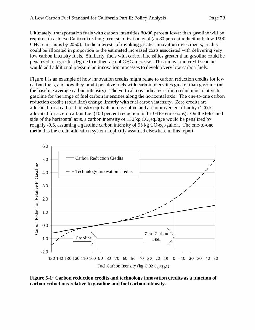
A Low Carbon Fuel Standard for California Part II: Policy Analysis Page 73
Ultimately, transportation fuels with carbon intensities 80-90 percent lower than gasoline will be required to achieve California’s long-term stabilization goal (an 80 percent reduction below 1990 GHG emissions by 2050). In the interests of invoking greater innovation investments, credits could be allocated in proportion to the estimated increased costs associated with delivering very low carbon intensity fuels. Similarly, fuels with carbon intensities greater than gasoline could be penalized to a greater degree than their actual GHG increase. This innovation credit scheme would add additional pressure on innovation processes to develop very low carbon fuels. Figure 1 is an example of how innovation credits might relate to carbon reduction credits for low carbon fuels, and how they might penalize fuels with carbon intensities greater than gasoline (or the baseline average carbon intensity). The vertical axis indicates carbon reductions relative to gasoline for the range of fuel carbon intensities along the horizontal axis. The one-to-one carbon reduction credits (solid line) change linearly with fuel carbon intensity. Zero credits are allocated for a carbon intensity equivalent to gasoline and an improvement of unity (1.0) is allocated for a zero carbon fuel (100 percent reduction in the GHG emissions). On the left-hand side of the horizontal axis, a carbon intensity of 150 kg CO2eq./gge would be penalized by roughly -0.5, assuming a gasoline carbon intensity of 95 kg CO2eq./gallon. The one-to-one method is the credit allocation system implicitly assumed elsewhere in this report.
-2.0
-1.0
0.0
1.0
2.0
3.0
4.0
5.0
6.0
150 140 130 120 110 100 90 80 70 60 50 40 30 20 10 0 -10 -20 -30 -40 -50
Fuel Carbon Inensity (kg CO2 eq./gge)
Car
bon
Red
uctio
n R
elat
ive
to G
asol
ine
Carbon Reduction Credits
Technology Innovation Credits
GasolineZero Carbon
Fuel
Figure 5-1: Carbon reduction credits and technology innovation credits as a function of carbon reductions relative to gasoline and fuel carbon intensity.

A Low Carbon Fuel Standard for California Part II: Policy Analysis Page 74
In contrast, innovation credits would be determined as a function of carbon intensity rather than GHG emissions and would serve as an additional incentive for very low carbon fuels. A hypothetical innovation credits system is indicated in Figure 5-1. One-to-one carbon reduction credits are shown as a solid line, and innovation credits, shown by the dotted line, exceed the one-to-one carbon reduction credits. Innovation credits increase more than linearly for very low carbon intensities, and serve as a penalty for very high carbon intensity fuels. Innovation credits have little influence on fuels with carbon intensities similar to gasoline. In the figure, the line indicating innovation credits has been set such that twice as many credits would be allocated for a zero carbon fuel, and five times more credit for a carbon intensity of -50 kg CO2 eq./gge. Similarly, a fuel with a carbon intensity of 150 kg CO2eq./gge would be penalized by -1.5 rather than -0.5 in the case of the one-to-one credit system. The innovation credits curve in Figure 5-1 is only shown here for the sake of discussion. Ideally, the actual structure of the innovation credit system would be based upon a comprehensive cost analysis of the investments required to develop different fuels across a wide range of carbon intensities. If the innovation credit system is structured such that the credits allocated exceed the predicted correlation between investment requirements and reduced carbon intensities, there would be an even greater incentive to deliver (and develop through R&D) very low carbon intensity fuels. Innovation credits could therefore have a greater influence across the RD3 pipeline discussed in section 2.2. While this cost analysis has yet to be completed, it seems likely that an innovation credit system such as that proposed here would more accurately reflect the underlying cost structure of very low carbon fuels than a one-to-one credit system. A deviation from a credit system based upon a direct one-to-one relationship between credits and GHG reductions introduces an accounting challenge. At first glance, it would appear that the proposed innovation credit system would result in more credits being allocated than the actual GHG reductions achieved. Below is one proposal for addressing this disparity. Normalize based upon total credits allocated. The total credits allocated in a given year, including both direct GHG and innovation credits, would be normalized by the corresponding absolute GHG reductions. This would restore a one-to-one relationship for the fuels produced by each regulated entity while incorporating credit for innovation. An interesting aspect of this accounting approach is that the value of credits would change depending upon the mix of carbon intensities of the fuels produced. For example, if one regulated entity sells a very low carbon fuel, a normalized credit system would reduce the relative value of the credits allocated for other fuels compared to the value of credits that would have been allocated in a simple one-to-one credit system. Uncertainty of compliance under this approach could be removed by allowing entities to comply with the LCFS on the basis of one-to-one credits, but allocating tradable credits that are the sum of both one-to-one GHG credits and carbon intensity innovation credits.

A Low Carbon Fuel Standard for California Part II: Policy Analysis Page 75
5.5 Environmental justice and sustainability issues
RECOMMENDATION 19: Fuel providers should be required to report on the sustainability impacts of their fuels, especially those related to biofuels. The state should perform a periodic assessment of the impacts of the LCFS, in California, the US and globally, and should consider policies and sustainability metrics to mitigate these effects as we learn about them. Biofuels produced on protected lands should be excluded from the LCFS. The ARB should conduct more research on sustainability impacts, paying close attention to international efforts. At the start of LCFS implementation, we recommend against regulatory requirements beyond the reporting and land exclusion provisions. At the mid-course review, the effectiveness of the reporting requirements should be evaluated and the adoption of additional sustainability metrics should be considered. The introduction of new fuels will affect the physical and human environment in many ways. The reality is that all forms of energy have downsides. If developed on a large scale, biofuels are likely to have substantial social and environmental impacts, which may vary substantially among feedstock and production processes. As California is becoming a leader in the development of alternative transportation fuels, it is important to understand the effect this expansion may have and to guide choices towards more sustainable biofuels. Many effects are likely to be dealt with by existing rules and policies, but some will not be. The sustainability issues associated with biofuels, in addition to degraded air and water quality, might include increased soil erosion, loss of biodiversity, use of genetically modified organisms, loss of wilderness and natural habitats, increased concentration of land holdings and land appropriation, reductions in worker safety, and increases in food prices. Many of these issues are also associated with other fuels, such as electricity or hydrogen, depending on energy resources and conversion technologies. These are very important issues today and will persist as important issues into the foreseeable future. However, they involve a wide range of factors and pose a number of different policy challenges. We suggest that the use of a global warming intensity metric in the LCFS is an effective surrogate for several of the sustainability concerns noted above, but not all. For example, in the case of biofuels, a reduction in global warming intensity through the LCFS generally improves sustainability because the two most important factors affecting this intensity—land use conversion and nitrous oxide emissions from soil—correlate well with other sustainability concerns. The LCFS, if it included land use conversion effects, would reduce biodiversity loss, soil erosion, and runoff of nutrients and pesticide. The LCFS would also reduce excess application of nitrogen fertilizer because its use results in emissions of nitrous oxide (a very potent greenhouse gas), as well as related water pollution and eutrophication. Social issues associated with sustainability are not so well captured by the LCFS. For example, conversion from food crops to biofuel crops can raise food prices. Further, an increase in biofuel production can lead to a consolidation of land holdings which could affect small land owners with little political power.

A Low Carbon Fuel Standard for California Part II: Policy Analysis Page 76
Climate change itself is an environmental justice issue, and many of the impacts of climate change are likely to fall more significantly on low income groups. This includes low-income groups in the United States as well as in other countries. For instance, heat waves that induce stress and increase mortality rates tend to affect populations that are unable to afford air-conditioning. Poorer people in developing countries are much more vulnerable to climate change. This is particularly true for people who rely on subsistence agriculture or live in coastal or low lying areas. What should be done about these sustainability effects and concerns? Unfortunately, there is no well-established, well-understood, or reliable method for measuring many of these effects. We recommend that the Air Resources Board conduct research on these effects, and develop methods and metrics for measuring and reporting on the sustainability of transportation fuels. Much effort is being given to such approaches in Europe. This will be a good opportunity to learn from the Europeans and to borrow from them. We recommend that a reporting requirement for sustainability impacts be imposed on fuel providers. We also recommend that the state conduct independent periodic assessments of the sustainability impacts of the LCFS policy. We recommend that this reporting include the impacts of biofuels production in California, as well as impacts throughout the US and globally. The global scale of the assessment is recommended since the global market for biofuels is affected by increased biofuel consumption in California, regardless of where the biofuel is produced. The assessment should include direct and indirect impacts, taking into account the indirect impacts this agriculture-based industry can have. If negative impacts of the LCFS are identified in the assessment, the state should take action to mitigate these impacts through means such as best management practices, incentives, regulation, and sustainability metrics. At the onset, we recommend that biofuels produced on certain types of land be prohibited, such as from old growth forest, national and state parks and other protected lands. Initially, we recommend against additional regulatory requirements regarding sustainability issues unrelated to greenhouse gas emissions. We believe that the LCFS should be kept as simple as possible in its early years as it is becoming established. As we better understand the potential impacts of biofuels production and the metrics and means for monitoring and avoiding these impacts, policymakers should consider including other sustainability impacts in the LCFS. Because sustainability will be a significant feature of European biofuel certification procedures, it is important that the California LCFS be deliberately compatible with international standards. This compatibility will be especially important in handling imports from elsewhere. The California LCFS can benefit from experiences and capabilities in Europe.
5.6 Regulatory capacity needed by the state
The California Air Resources Board will require additional resources to carry out the LCFS. This includes both financial resources as well as trained staff. It is imperative that neither the administration nor the legislature expect LCFS administration to be a peripheral set of duties that can be shoehorned into current operations without explicit funding. At several points in this report we have pointed out questions that require further study, much of which is probably best done extramurally by contract, and this will also require funding.

A Low Carbon Fuel Standard for California Part II: Policy Analysis Page 77
The ARB is not alone in administering the LCFS. The State of California already has considerable regulatory capacity. As mentioned above, the Board of Equalization already has systems in place for the collection of fuel taxes that may be suitable for, possibly with modification, the LCFS. In addition, the California Energy Commission manages the Petroleum Industry Information Reporting Act (PIIRA) program. Enacted in 1980, PIIRA requires qualifying petroleum industry companies to submit weekly, monthly, and annual data to the California Energy Commission. Data collection began in 1982. In 2006, the PIIRA regulations were amended to increase the frequency and level of detail in the information reported by the industry. The reports required by PIIRA are filed by businesses that ship, receive, store, process, and sell crude oil and petroleum products in California (petroleum products include gasoline, diesel, jet fuel, and blending components). Thus, all the obligated parties in the LCFS already submit detailed reports to the PIIRA program. Importantly, the Energy Commission holds confidential the data reported by individual companies under PIIRA. The Energy Commission aggregates the data to ensure confidentiality of information about individual companies. The aggregated information is published in a variety of Energy Commission reports. This may be important for the LCFS because data to certify the carbon intensity of fuels may be considered proprietary and would require the sort of handling that the PIIRA program already provides.
5.7 Program review
RECOMMENDATION 20: Conduct a 5 year review, beginning in 2013, of data, methods, fuel production technologies, and advanced vehicle technologies. The intent is not to review the intensity targets, unless climate science has so radically changed that we are much more confident than today that either greater or lesser reductions are required. We strongly recommend a mid-program review -- around 2013, to assure that changes can be implemented in 2015. Such a review is important because much new knowledge will be gained about climate science, fuel production, vehicle technologies, climate impacts, and the various methods, tools, and institutions put in place to implement the LCFS. We do not recommend more frequent reviews because the focus should be on tools, data, measurement, and efficacy. This timing would allow for considerable research and development in both methodologies for measuring life cycle emissions and new fuel technologies. By this time, the current DOE cellulosic ethanol pilot projects will be in operation for several years, providing considerable insights into how well these technologies are working. Other research projects currently starting will have significant results by this time, including efforts to improve LEM and GREET, and the large UC Davis and UC Berkeley biofuel research initiatives. The purpose of this review is not to delay, pause, or provide regulatory relief, sometimes referred to as “safety valves” and “off ramps.” The LCFS is being designed with considerable flexibility, so as to obviate the need for regulatory relief. The review should not change the targets unless

A Low Carbon Fuel Standard for California Part II: Policy Analysis Page 78
the climate science has so radically changed that we are much more confident than today that either greater or lesser reductions are required. We also recommend that there be only one program review after 5 years. It should not be biennial. Routine reviews incur large burdens on the resources of regulatory agencies. Concerns voiced by some stakeholders that that the LCFS might be “not working” or “going the wrong way” are best addressed by ensuring competition among technologies and firms so that if one particular firm is unable to meet its obligation, others can do so. Through trading of credits, emissions will be reduced by others. Alternatively, an obligated firm could pay a fee as a legitimate compliance mechanism. The state could use the fees to support the objectives of the LCFS, but until results are observed, these fees cannot be assumed; the industry may well find it possible to meet LCFS targets with trading and technological change alone. The possible receipt of significant fees raises two policy issues. First, if significant revenues were to flow in from this source, what account should they be held in and to what purposes should they be put? The optimal use would be to purchase transportation-sector GHG emission reduction credits.35
5.8 Cost analysis
RECCOMENDATION 21: The ARB should conduct a cost analysis of the LCFS following the cost-effectiveness approach used in evaluating the U.S. Clean Air Act. This analysis should acknowledge uncertainties due to proprietary information and innovation in low-carbon energy technologies. It should also include a discussion of non-climate related costs and benefits. CARB is required to conduct a cost assessment of new regulations and will do so with the LCFS. The purpose of such an analysis should be to evaluate the cost-effectiveness of the proposed regulations, following the approach embodied in the U.S. Clean Air Act, which the U.S. Supreme Court ruled provides a legal basis for state regulation of greenhouse gases (Massachusetts vs. EPA). The key principal is to protect human health and the environment with an adequate margin of safety, in this case by protecting against climate change. Cost analysis follows determinations of the actions needed to achieve such standards. Thus, CARB’s cost analysis of the LCFS should evaluate the cost-effectiveness of achieving the carbon intensity reduction specified by the regulation, but not the emission reduction goals set into place by law or regulation. The U.S. Supreme Court has repeatedly ruled that the Clean Air Act prohibits subjecting such goals to cost-benefit tests. The many co-benefits of the LCFS (notably reductions in oil imports), should also be included in this analysis. Cost analyses are crucial for understanding how best to achieve the goals set out by legislation, and to provide information for government to use in determining if and when additional support might be needed for particular fuel options (for instance to overcome startup barriers or market imperfections).
35 The administrative costs of the LCFS program should not be paid for by these fees. This is a seductive idea but
contrary to public finance and economic principles, because the need for operating the LCFS program is not related the income it generates through fees (O’Hare, 2006). Indeed, a successful LCFS program would generate no fees whatsoever. LCFS program costs should be covered by general fund revenues.

A Low Carbon Fuel Standard for California Part II: Policy Analysis Page 79
Conducting a thorough cost analysis of the LCFS will prove to be a challenging endeavor. Any cost analysis study should take into consideration all cost data available from reliable sources. Some of this data will be empirical, some may be proprietary, and some will include estimates of future costs. Integrating this data into a consistent cost analysis framework that includes the range of options available for meeting the LCFS will prove challenging for at least 3 reasons: 1) the uncertainty of future costs estimates, especially those associated with technologies that have yet to be commercialized, 2) the inevitable stakeholder disputes that will arise from any choice of representative costs, and 3) the variety of perspectives on what constitutes cost effectiveness. Each is discussed briefly below. While empirical studies of historical cost reductions achieved through learning-by-ding offer support for analytic methods of projecting future costs (e.g., using experience curves, as described in Wene 2000), any projections of the future involve uncertainties. These uncertainties will be especially difficult to resolve when comparing multiple technological options, some of which may experience a greater degree of innovation (and therefore cost reduction) over time than others. If the open process of developing the LCFS continues to rely upon input from a wide range of stakeholders, any estimates of representative values will likely be challenged by someone as being too high or too low. Advocates of a particular technology will inevitably offer persuasive arguments and analysis explaining why their technology will be more competitive relative to other technologies. Some of these analyses will contain valuable data that could contribute to the rigor of the cost study. Others will be exaggerated. Sifting through all available data and incorporating only the high quality data will inevitably prove challenging, and follows from the information asymmetry between those conducting the analysis and the industry stakeholders who are most familiar with the costs of particular technologies. We recommend that any future cost analysis of the LCFS be conducted with the goal of determining what the most cost effective options are for meeting the 2020 goal. As explained elsewhere, the 2020 goal is only one step toward the much lower carbon intensities that must be achieved in order to approach climate stabilization by 2050 (see Part I, Section 1.5). Due to the many uncertain factors involved in both abatement costs and damage costs, the goal of the cost analysis should not be to determine what actions are warranted by setting projected costs equal to estimates damages due to climate change. While such a cost-benefit framework can be applied to this problem, the approach is inappropriate and the results would not be useful in guiding policy. In contrast, a precautionary approach is warranted, similar in spirit to the threshold goals of the Clean Air Act: to protect human health within an “ample margin of safety”. In summary, an analysis of least cost low carbon fuel options can help to inform California policymakers and potentially improve the design and implementation of the LCFS. However, the carbon intensity reductions required of the transportation sector in California to achieve climate stabilization should be consistent with global goals to address climate change. While we have not specifically addressed cost-effectiveness, the authors of this report are among the leading experts in alternative fuel analyses and have considerable knowledge of costs. The scenarios created in Part 1 reflect judgments about which fuels are likely to be most cost competitive in the coming years. Our collective judgment is that the 10 percent target is attainable by 2020 without extraordinary cost. What are uncertain are the rate of innovation for different technologies, and the acceptance of those technologies and fuels by customers.

A Low Carbon Fuel Standard for California Part II: Policy Analysis Page 80
5.9 Research needs
RECCOMENDATION 22: A great deal of research is needed to successfully implement the LCFS. Key areas include better characterization of the global warming impacts of different fuels, tools to allow regulators and obligated parties to assess different fuel production pathways, uncertainties in these values, the role of land use, environmental justice and sustainability goals, and the GHG implications of the vehicle lifecycle. Successful implementation of the LCFS will require continued research and development. Most critical is much more research into the development of competitive low-carbon fuels. Investments have been increasing in the past few years, but still lag what is needed. Much more concentrated effort to develop technologies is needed by government and especially by industry. But that is not the focus of this sub-section. Here we address the need for research to support the development of the LCFS program. An important component of this research will be the accurate characterization of the global warming intensity of all the major production pathways for each fuel. This characterization must be integrated into the LCFS regulatory framework as these new fuels enter the marketplace. A second key area of research is development of regulatory tools to specify life cycle impacts of the fuels. None of the existing models, including GREET, LEM and GHGenius, are fully acceptable. Those models sometimes generate quite different numbers. It appears that only a small number of factors make up for the largest differences between the results of these models. The most important factors are the following: how the effects of land-use changes are measured, emissions of nitrous oxide (N2O) and black carbon, and the appropriate averaging times for measuring global warming effects. The Air Resources Board should be able to determine appropriate values for these parameters for regulatory use in the first compliance period (2010 to 2015) relatively quickly. Continued research on improved estimates of these parameters and others used in life cycle assessment is important and should be pursued. Improved values can be used to update compliance methods and compliance strategies, just as in other typical regulatory processes. A closely related area of research is on uncertainties and variation associated with the measurement of global warming intensity of fuels. By variation, we refer to the fact that current life cycle assessments are typically based on self-reported average values aggregated over large areas, states or sometimes the entire nation. Agricultural data collected by the USDA’s National Agricultural Statistics Service (NASS) and Economic Research Service (ERS) underlie all major life cycle analyses of the two major biofuels produced in the US: corn ethanol and soybean biodiesel. USDA reports these data as averages for each parameter (e.g. agrichemical application rates, yield, on-farm energy use, incidence of no-tillage) as if the parameters were independent, when it is likely that some of these values are highly correlated. This leads to several problems. All prior attempts to estimate average greenhouse gas emissions are demonstrably incorrect as they are based on the independent averages of correlated parameters. We cannot compute the uncertainty of the result. Because the parameters are not independent, we cannot assign independent probability distributions to them for use in a Monte Carlo simulation. We cannot determine the effect on greenhouse gas emissions of practices such

A Low Carbon Fuel Standard for California Part II: Policy Analysis Page 81
as irrigation or no-till. Research to help resolve these issues will improve the quality of carbon intensity measurements. Research into the land use change implications of all fuel production, but in particular biofuel production, is also greatly needed. One major concern, referred to briefly in the discussion of land use change effects, is the development of appropriate frameworks for analyzing and regulating the land-use implications of fuel production. Current approaches such as that embodied in GREET are static, extremely simple, and based on old data. One possible solution would be to develop a meta-model that links life cycle assessment and macroeconomic models to predict indirect land-use changes (Delucchi 2004). However, this seems a daunting task, given the enormous data gaps, model uncertainty, deep uncertainties about future policies, prices, and technologies. In particular, this approach is likely to have very limited application in a regulatory context. Therefore better methods for the analysis and regulation of indirect land use change effects are required. Research is also needed, as indicated above, to understand and specify other sustainability and environmental justice goals. There is currently no agreed upon national or international definition of these issues or methods with which to measure them. Multiple organizations are developing or have recently developed criteria and indicators that may be useful for understanding how fuel production and use affect sustainability and environmental justice (Turner et al. 2007). More research on these issues and how fuel production can be better regulated to achieve greater levels of sustainability and environmental justice is required. Still other research should be pursued to analyze life cycle GHG emissions more broadly than addressed in this report. Here, we address only emissions from the fuel cycle. But the actual emissions associated with any fuel pathway are more extensive. They include emissions from the manufacturing of production facilities and the vehicles that use those fuels. Generally, the incremental emissions associated with one fuel pathway over another is probably small. But there may be some cases where they are large. For instance, it may be that the embodied energy in the materials – and therefore GHG emissions -- used in building some fuel production facilities may be large. Or it may be that the GHG emissions associated with the manufacture (and disposal) of some fuel cells or batteries might be large. Evaluating these effects and what the correct role (if any) in regulating them is an important research task.

A Low Carbon Fuel Standard for California Part II: Policy Analysis Page 82
(This page is intentionally blank.)

A Low Carbon Fuel Standard for California Part II: Policy Analysis Page 83
6 References Adelman, M. 1993. The Economics of Petroleum Supply. Cambridge, MA: The MIT Press.
Alic, John A. 1999. Technology Policies for Reducing Greenhouse Gas Emissions: A Taxonomy. Washington, D.C.: H. John Heinz III Center for Science, Economics and the Environment.
Baker, John M., Tyson E. Ochsner, Rodney T. Venterea, and Timothy J. Griffis. 2007. Tillage and soil carbon sequestration--What do we really know? Agriculture, Ecosystems & Environment 118 (1-4):1-5.
Bandivadekar, A.P., and J.B. Heywood. 2004. Coordinated Policy Measures for Reducing the Fuel Consumption of the U.S. Light-Duty Vehicle Fleet: MIT Energy Lab.
Bauen, A., J. Howes, and M. Franzosi. 2006. A methodology and tool for calculating the carbon intensity of biofuels. London: E4tech, ECCM, Themba.
Bauen, A., Philip Watson, and J. Howes. 2006. DRAFT Methodology for Carbon Reporting under the Renewable Transport Fuel Obligation. London: E4Tech.
———. 2006. Methodology for Carbon Reporting under the Renewable Transport Fuel Obligation. London: E4Tech.
Bemis, Gerry. 2006. Inventory of California Greenhouse Gas Emissions and Sinks: 1990 to 2004. Sacramento: California Energy Commission.
Borenstein, Severin, James Bushnell, and Matthew Lewis. 2004. Market Power in California's Gasoline Market. In Center for the Study of Energy Markets. Berkeley: University of California.
BCG, 1968. Perspectives on experience. Boston Consulting Group Inc.
BP (2007) Statistical Review of World Energy. London. www.bp.com
Brandt, Adam R., and Alexander E. Farrell. 2006. Scraping the bottom of the barrel: CO2 emissions consequences of a transition to low-quality and synthetic petroleum resources. Climatic Change Forthcoming.
Brown, M.A., 2001. Market failures and barriers as a basis for clean energy policies. Energy Policy 29, 1197-1207.
de Carvalho Macedo, I., M. Verde Leal, et al. (2004). Assessment of greenhouse gas emissions in the production and use of fuel ethanol in Brazil. Sao Paulo, Secretariat of the Environment, Government of the State of Sao Paulo, Available at http://www.unica.com.br/i_pages/files/gee3.pdf.
Damen, K., A. Faaij, F. van Bergen, J. Gale, and E. Lysen. 2005. Identification of early opportunities for CO2 sequestration-worldwide screening for CO2-EOR and CO2-ECBM projects. Energy 30 (10):1931-1952.
Davis, D.H., 1993. Energy Politics, Fourth. St. Martin's Press, New York.

A Low Carbon Fuel Standard for California Part II: Policy Analysis Page 84
DeCanio, Stephen J. 2003. Economic Models of Climate Change: A Critique. New York: Palgrave McMillan.
Delucchi, Mark A. 2004. Conceptual and Methodological Issues in Lifecycle Analyses of Transportation Fuels. In Institute of Transportation Studies. Davis: University of California.
Department for Transport. 2006. Consultation On The Draft Renewable Transport Fuel Obligations Order 2007. London: UK Department for Transport.
Dry, M. E. 2002. The Fischer-Tropsch process: 1950-2000. Catalysis Today 71 (3-4):227-241.
E4Tech. 2007. Carbon Reporting under the Renewable Transport Fuel Obligation: Technical Guidance (First Draft): E4Tech.
Elliott, S., K. S. Lackner, H. J. Ziock, M. K. Dubey, H. P. Hanson, S. Barr, N. A. Ciszkowski, and D. R. Blake. 2001. Compensation of atmospheric CO2 buildup through engineered chemical sinkage. Geophysical Research Letters 28 (7):1235-1238.
Ellis, J., H. Winkler, J. Corfee-Morlot, and F. Gagnon-Lebrun. 2007. CDM: Taking stock and looking forward. Energy Policy 35 (1):15-28.
Energy Information Administration. 2001. Analysis of Strategies for Reducing Multiple Emissions from Electric Power Plants with Advanced Technology Scenarios. Washington, DC: U.S. Department of Energy.
———. 2003. 2003 California Gasoline Price Study. Washington, DC: U.S. Department of Energy.
———. 2007. Energy Market and Economic Impacts of a Proposal to Reduce Greenhouse Gas Intensity with a Cap and Trade System. Washington, DC: U.S. Department of Energy.
Energy Policy Act of 2005. Public Law 109-58. Aug 8, 2005. 109th Congress.
EPA. 2007. 40 CFR Part 80: Regulation of Fuels and Fuel Additives: Renewable Fuel Standard Program: Final Rule. Washington, DC: Environmental Protection Agency.
Falola, Toyin, and Ann Genova. 2005. The Politics of the Global Oil Industry. Westport, CT: Praeger.
Farrell, Alexander E., and Lester B. Lave. 2004. Emission Trading and Human Health. Annual Review of Public Health 25:119-138.
Feddema, J. J., K. W. Oleson, et al. (2005). "The importance of land-cover change in simulating future climates." Science 310(5754): 1674-1678.
Gately, D. 2004. OPEC's incentives for faster output growth. Energy Journal 25 (2):75-96.
Gibbard, S. K. Caldiera, G. Bela, T. Philips, M. Wickett. (2005) Climate effects of global land cover change. Geophysical Research Letters. 32.
Greene, David L., Philip D. Patterson, Margaret Singh, and Jia Li. 2005. Feebates, rebates and gas-guzzler taxes: a study of incentives for increased fuel economy Energy Policy 33 (6):757-775.
Hahn, Robert. 1989. Economic Prescriptions for Environmental Problems: How the Patient Followed the Doctor's Orders. Journal of Economic Perspectives 3 (2):95-114.

A Low Carbon Fuel Standard for California Part II: Policy Analysis Page 85
Heavenrich, Robert M. 2006. Light-Duty Automotive Technology and Fuel Economy Trends: 1975 Through 2006. In Office of Transportation and Air Quality. Washington, DC: U.S. Environmental Protection Agency.
Heffner, Reid, Kenneth S. Kurani, and Thomas S. Turrentine. 2007. Symbolism in early markets for hybrid electric vehicles. In Institute for Transportation Studies. Davis: University of California.
Hess, D. B., and P. A. Lombardi. 2004. Policy support for and barriers to transit-oriented development in the inner city - Literature review. In Transit Planning and Development, Management and Performance, Marketing and Fare Policy, and Capacity and Quality of Service.
Holland, Stephen P., Christopher R. Knittel, and Jonathan E. Hughes. 2007. Greenhouse Gas Reductions under Low Carbon Fuel Standards? In Center for the Study of Energy
Houghton, R. A. (2003). "Why are estimates of the terrestrial carbon balance so different?" Global Change Biology 9(4): 500-509.
Houghton, R. A. 1999. The annual net flux of carbon to the atmosphere from changes in land use 1850-1990*. Tellus B 51 (2):298-313.
Intergovernmental Panel on Climate Change. 2005. IPCC Special Report on Carbon dioxide Capture and Storage. Cambridge: University of Cambridge Press.
Jessen, K., A. R. Kovscek, and F. M. Orr. 2005. Increasing CO2 storage in oil recovery. Energy Conversion and Management 46 (2):293-311.
Kavalec, C., J. Page, and L. Stamets. (2005) Forecasts of California Transportation Energy Demand 2005-2025. California Energy Commission. April. CEC-600-2005-008. 11 pp.
Keith, D. W., M. Ha-Duong, and J. K. Stolaroff. 2006. Climate strategy with CO2 capture from the air. Climatic Change 74 (1-3):17-45.
Lackner, K. (2002) Carbonate chemistry for sequestering fossil carbon? Annual Review of Energy and the Environment.27: 193-232.
Lemoine, Derek, Daniel M. Kammen, and Alexander E. Farrell. 2006. Effects of PHEVs on Electricity and Gasoline Markets. Under review.
Levine, Jonathan. 2006. Zoned Out: Regulation, Markets, and Choices in Transportation and Metropolitan Land-Use. Washington, DC: RFF Press.
Lockyear, Bill 2000. Attorney General's Report on Gasoline Pricing In California. Sacramento: Office of the Attorney General.
Market Advisory Committee. (2007) Recommendations for Designing a Cap-and-Trade System for California. California Air Resources Board. June 30. 109 pp. http://www.climatechange.ca.gov/policies/market_advisory.html
Marland, G., R. A. Pielke, et al. (2003). "The climatic impacts of land surface change and carbon management, and the implications for climate-change mitigation policy." Climate Policy 3(2): 149-157.
Martini, John. 2007. Letter from California Independent Petroleum Association. Sacramento.

A Low Carbon Fuel Standard for California Part II: Policy Analysis Page 86
Mathews, John A. 2007. Biofuels: What a Biopact between North and South could achieve. Energy Policy In Press, Corrected Proof.
McCarl, B. A., and R. D. Sands. 2007. Competitiveness of terrestrial greenhouse gas offsets: are they a bridge to the future? Climatic Change 80 (1-2):109-126.
Melaina, M.W., 2003. Initiating hydrogen infrastructures: preliminary analysis of a sufficient number of initial hydrogen stations in the U.S. International Journal of Hydrogen Energy 28, 743-755.
NCGA (2007). 2007 World of Corn. Chesterfield, MO, National Corn Growers Association, Available at http://www.ncga.com/WorldOfCorn/main/.
Nicholas, M.A., Handy, S.L., Sperling, D., 2004. Using Geographic Information Systems to Evaluate Siting and Networks of Hydrogen Stations. Transportation Research Record 1880, 126-134.
Norberg-Bohm, V., Ed. 2002. The Role of Government in Energy Technology Innovation: Insights for Government Policy in the Energy Sector. BSCIA Working Paper 2002-14, Energy Technology Innovation Project, Belfer Center for Science and International Affairs.
O'Hare, Michael, and David S. Mundel. 1983. When to Pay for Sunk Benefits. In What Role for Government?: Lessons from Policy Research, edited by D. Leebaert and R. Zeckhauser. Durham, NC: Duke University Press.
Parry, Ian W. H. 1998. A Second Best Analysis of Environmental Subsidies. International Tax and Public Finance 5:157-174.
Parson, Edward A., and David W. Keith. 1998. Fossil Fuels Without CO2 Emissions. Science 282:1053-1054.
PCAST, 1999. Powerful Partnerships: The Federal Role in International Cooperation on Energy Innovation. President's Committee of Advisors on Science and Technology, Washington, D.C.
Plevin, R. J. 2006. California Policy Should Distinguish Biofuels by Differential Global Warming Effects, Energy and Resources Group, U. of California-Berkeley, Berkeley.
Potter, C. S. (1999). "Terrestrial biomass and the effects of deforestation on the global carbon cycle - Results from a model of primary production using satellite observations." Bioscience 49(10): 769-778.
Quirion, P. 2005. Does uncertainty justify intensity emission caps? Resource and Energy Economics 27 (4):343-353.
Reheis-Boyd, Catherine. 2007. Letter from Western States Petroleum Association. Sacramento.
Romm, Joseph J., and Andrew A. Frank. 2006. Hybrid Vehicles Gain Traction. Scientific American, April, 72-79.
Ross, M., 1986. Capital budgeting practices of twelve large manufacturers. Financial Management 15, 15-22.
Schimel, D. S., J. I. House, K. A. Hibbard, P. Bousquet, P. Ciais, P. Peylin, B. H. Braswell, M. J. Apps, D. Baker, A. Bondeau, J. Canadell, G. Churkina, W. Cramer, A. S. Denning, C. B.

A Low Carbon Fuel Standard for California Part II: Policy Analysis Page 87
Field, P. Friedlingstein, C. Goodale, M. Heimann, R. A. Houghton, J. M. Melillo, B. Moore, D. Murdiyarso, I. Noble, S. W. Pacala, I. C. Prentice, M. R. Raupach, P. J. Rayner, R. J. Scholes, W. L. Steffen, and C. Wirth. 2001. Recent patterns and mechanisms of carbon exchange by terrestrial ecosystems. Nature 414 (6860):169-172.
Schwarzenegger, Arnold. 2007. Executive Order S-01-07: Low Carbon Fuel Standard. Sacramento, CA.
Scotchmer, S., Innovation and Incentives. 2006. MIT Press Cambridge, MA.
Sheridan, Magaret. 2006. California Crude Oil Production and Imports. Sacramento: California Energy Commission.
Stern, Nicholas, S. Peters, V. Bakhshi, A. Bowen, C. Cameron, S. Catovsky, and D Crane. 2006. Stern Review: The Economics of Climate Change. London: HM Treasury.
Stolaroff, J. K., G. V. Lowry, and D. W. Keith. 2005. Using CaO- and MgO-rich industrial waste streams for carbon sequestration. Energy Conversion and Management 46 (5):687-699.
Tilman, David A., Jason Hill, and Clarence Lehman. 2006. Carbon-Negative Biofuels from Low-Input High-Diversity Grassland Biomass. Science 314:1598-1600.
Tol, Richard S. J. 1999. The Marginal Costs of Greenhouse Gas Emissions. Energy Journal 20 (1):61-81.
Turner, Brian T., Richard J. Plevin, Michael O'Hare, and Alexander E. Farrell. 2007. Creating Markets for Green Biofuels. In Transportation Sustainability Research Center. Berkeley: University of California.
Turrentine, Thomas S., Mark A. Delucchi, Reid Heffner, Kenneth S. Kurani, and Yongling Sun. 2006. Quantifying the Benefits of Hybrid Vehicles. In Institute of Transportation Studies. Davis: University of California.
Unnasch, Stefan, Michael Chan, Larry Waterland, Jennifer Pont, Matthew Hooks, and Daniel Rutherford. 2007. Full Fuel Cycle Assessment Tank To Wheels Energy Inputs, Emissions, And Water Impacts. Sacramento: California Energy Commission.
Unnasch, Stefan, Jennifer Pont, Michael Chan, and Larry Waterland. 2007. Full Fuel Cycle Assessment Well To Wheels Energy Inputs, Emissions, And Water Impacts. Sacramento: California Energy Commission.
US EPA. 2007. Regulation of Fuel and Fuel Additives, edited by U.S. Environmental Protection Agency.
Watson, Philip. 2007. Email exchange with Richard Plevin. Berkeley.
Weyant, John P., and Jennifer Hill. 1999. The Costs Of The Kyoto Protocol: A Multi-Model Evaluation. The Energy Journal Special Issue:398.
Wene, C., 2000. Experience curves for energy technology policy. Organisation for Economic Co-operation and Development, International Energy Agency, Paris.
Williams, Brett D., and Kenneth S. Kurani. 2007. Commercializing light-duty plug-in/plug-out hydrogen-fuel-cell vehicles: “Mobile Electricity” technologies and opportunities. Journal of Power Sources 166 (2):549-566.

A Low Carbon Fuel Standard for California Part II: Policy Analysis Page 88
Williams, Robert H., Eric D. Larson, and Haiming Jin. 2006. Synthetic fuels in a world with high oil and carbon prices. Paper read at 8th International Conference on Greenhouse Gas Control Technologies, at Trondheim, Norway.
Winebrake, James J., and Alex Farrell. 1997. The AFV Credit Program and Its Role in Future AFV Market Development. Transportation Research D 2 (2):125-132.
Wang, M. Q. (2006, January 2006). "GREET 1.7 (beta) Spreadsheet Model." from http://www.transportation.anl.gov/software/GREET/.

A Low Carbon Fuel Standard for California Part II: Policy Analysis Page 89
Appendix A: VISION-CA scenarios with indirect land use change Appendix A. VISION-CA Scenarios with indirect land use change In order to better understand the potential influence of land use change (LUC) effects on the carbon intensity of different fuels, and their capacity to contribute to AFCI reduction goals, scenarios G10 and H10 have been revisited. Estimates for increased carbon intensities for (average) corn ethanol, mid-GHG biofuels and biodiesel due to LUC effects are discussed in section 4.5. In the scenario variations below, the carbon intensities of corn ethanol and mid-GHG biofuel have been increased by 22 and 15 g CO2e/MJ, respectively. Because the LUC estimates for biodiesel are so large (96 g CO2e/MJ), biodiesel has been removed from scenario G10. See section 4.5.3 for a summary of these scenario variations, and compare the H10* and G10* scenarios with the original G10 and H10 scenarios from Part I of the UC LCFS report. Variation G10* of the Biofuel Intensive Scenarios In this scenario a mid-GHG ethanol is introduced for both FFVs and as a blend in gasoline. The number of FFVs is increased and the frequency of refueling these vehicles with biofuels is increased. Biodiesel and a low-GHG FT diesel fuel blend are introduced and the number of diesel vehicles sold per year increases. Scenario G10* Assumptions • Assumption #1. Introduce mid-GHG Ethanol (5.7% vol.).
A mid-GHG biofuel is introduced as a blend for gasoline, displacing today’s average-GHG intensity ethanol over time. By 2010, 10 percent of the gasoline blend component is a mid-GHG intensity biofuel, and 65 percent is a mid-GHG biofuel by 2020.
• Assumption #2. Increase biofuel blend to 10% by vol.
The quantity of biofuel blended with gasoline is increased to 10 percent by volume, maintaining the fraction of mid-GHG biofuel from assumption #1
• Assumption #3. Increase number of FFVs
The number of FFVs sold is increased to approximately 800,000 per year by 2020. This assumption is consistent with recent declarations by U.S. automakers of their capability to increase the percentage of ethanol-capable FFVs to half of all vehicles produced by 2012 (see assumption #7 in Scenario F10).
• Assumption #4. Increase FFV biofuel VMT to 50 percent
The frequency of refueling existing FFVs with biofuel (e.g., ethanol) is increased such that 50 percent of all VMT are driven on an 85 percent vol. blend with the carbon intensity defined in assumption #1. This assumption brings the AFCI value for Scenario G5 to 0.95.
• Assumption #5. Introduce low-GHG biofuel In assumption #1, a mid-GHG biofuel was introduced for the biofuel blend component of gasoline. The present assumption is that 5 percent of this blend component is supplied as a low-GHG biofuel by 2010, and 30 percent by 2020.

A Low Carbon Fuel Standard for California Part II: Policy Analysis Page 90
• Assumption #6. Introduce low-GHG FT diesel A low-GHG FT diesel blend is introduced in addition to the biodiesel blend from assumption #3. The low-GHG FT diesel is blended at 2 percent by vol. in 2010 and 20 percent by vol. by 2020.
• Assumption #7. Increase sales of diesel fuel
The number of diesel vehicles sold per year increases exponentially beginning around 2010. By 2030, over 750,000 new LDVs sold per year are diesel vehicles. These vehicles operate on the diesel blend defined in assumptions #3 and #7.

A Low Carbon Fuel Standard for California Part II: Policy Analysis Page 91
0.0
0.2
0.4
0.6
0.8
1.0
1.2
1.4
1.6
1.8
2.0
2000 2005 2010 2015 2020
Bill
ions
GG
E (a
lt fu
els
only
Diesel
CNG
Biofuel blend
Biofuel (85%)
F-T Diesel
Bio-Diesel
Hydrogen
Electric
Figure A1: Fuel energy consumption in Scenario G10*
0
100
200
300
400
500
600
700
800
900
1,000
2000 2005 2010 2015 2020
New
LD
Vs
Sol
d (1
000s
)
SI HEV
Diesel
D HEV
Bio FFV
CNG
SI PHEV
D PHEV
FFV HEV
FCV
EV
New Gasoline ICE LDVs Sold in 2020:
0.7 million
Figure A2: New LDVs sold per year in Scenario G10*

A Low Carbon Fuel Standard for California Part II: Policy Analysis Page 92
Table A1: Fuel energy, GHG intensities, AFCI values & GHG emissions for Scenario G10* SCENARIO: Biofuel Intensive (G10) 2005 2010 2015 2020 Fuel Energy Consumption by Type Total Fuel Energy LDVs (Billion GGE) 15.929 17.097 17.494 16.991 Gasoline 15.101 15.934 15.609 13.242 Diesel 0.230 0.249 0.496 1.255 CNG 0.013 0.016 0.021 0.026 F-T Diesel 0.0 0.005 0.061 0.314 Bio-Diesel 0.0 0.0 0.0 0.0 Methanol 0.0 0.0 0.0 0.0 Hydrogen 0.0 0.0 0.0001 0.0016 Electric 0.0001 0.0005 0.0011 0.0066 Ethanol (blended) 0.585 0.831 0.978 1.017 Ethanol (85% vol.) 0.0 0.061 0.328 1.128 Fuel GHG Intensities Average for all fuels (g CO2 eq/MJ) 93.6 93.3 91.5 86.7 Gasoline (with biofuel blend) 93.7 93.4 92.2 90.6 Diesel 91.6 90.0 82.9 75.7 CNG 68.1 68.1 68.1 68.1 Hydrogen 0.0 0.0 107.7 107.7 Electric 121.5 121.5 121.5 121.5 Ethanol (85% vol.) 97.9 90.6 71.9 53.2 AFCI Values Average for all fuels 1.0 0.996 0.970 0.901
Change from BAU (%) -0.3% -2.3% -8.2% Gasoline (with biofuel blend) 1.0 0.997 0.985 0.970 Diesel 0.764 0.725 0.594 0.529 CNG 0.694 0.682 0.671 0.660 Hydrogen - - - 0.526 Electric 0.347 0.270 0.249 0.239 Ethanol (85% vol.) 1.0 0.994 0.934 0.825 Total GHG Emissions All LDVs (MMT CO2 eq.) 196.6 210.3 211.2 194.4
Table A2: Sales of LDVs for Scenario G10*
SCENARIO: Biofuel Intensive (G10) 2005 2010 2015 2020 New Light Duty Vehicle Sales New LDV Sales (millions) 1.949 2.096 2.209 2.323 Gasoline ICE 1.838 1.769 1.358 0.700
Change from BAU (%) -1.9% -19.4% -56.0% Battery EVs 0.0 0.001 0.001 0.001 Ethanol ICE FFVs 0.064 0.166 0.438 0.805 Diesel 0.023 0.058 0.233 0.593 CNG 0.001 0.003 0.003 0.003 Gasoline SI HEV 0.022 0.099 0.174 0.208 E85 SI HEV 0.0 0.0 0.0 0.0 Diesel HEV 0.0 0.0 0.0 0.0 Gasoline SI PHEV 0.0 0.0 0.002 0.012 Diesel PHEV 0.0 0.0 0.0 0.0 Hydrogen FCV 0.0 0.0 0.0 0.001

A Low Carbon Fuel Standard for California Part II: Policy Analysis Page 93
Variation H10* of the Multiple Fuel and Vehicle Scenarios This scenario combines multiple fuels and vehicle technologies. The scenario is constructed with assumptions similar to those used in other scenarios, but they are combined in a unique sequence that begins with a low-GHG biofuel blend, introduces CNG and electric drive vehicles (at more modest rates than in the Electric Drive scenario), and attains final AFCI reductions by increasing volumes of low-GHG biofuel and low-GHG FT diesel. Scenario H10* Assumptions • Assumption #1. Introduction of a low-GHG Biofuel (5.7% vol.)
A low-GHG biofuel is introduced as a 5.7% blend in gasoline. The fraction of the blend composed of this new biofuel increases to 10% by 2010 and 30% by 2020.
• Assumption #2. Increase biofuel blend to 10% by vol.
The biofuel blend in gasoline is increased to 7.5% by 2010 and 10% by 2020. The GHG intensity is the same as defined in assumption #1.
• Assumption #3. Increase number of CNG vehicles
The new LDV market share for CNG vehicles begins to increase rapidly after 2015. New CNG vehicles sales reach 94,000 by 2020.
• Assumption #4. Introduce of PHEVs
The new LDV market share for PHEVs begins to increase rapidly after 2010. By 2020, 172,000 PHEVs are sold per year. This assumption brings the AFCI to 0.95 for scenario H5.
• Assumption #5. Introduce low-GHG FT diesel
A low-GHG FT diesel is blended with diesel fuel at 5% by 2010 and 20% by 2020. This fuel is consumed by the same number of diesel vehicles on the road in the BAU scenario.
• Assumption #6. Increase biofuel sales to FFVs
Now the number of FFVs increases to over 800,000 per year. This assumption is consistent with recent declarations by U.S. automakers of their capability to increase the percentage of ethanol-capable FFVs to half of all vehicles produced by 2012 (see assumption #7 in scenario F10).
• Assumption #7. Increase FFV biofuel VMT to 50%
The frequency of refueling existing FFVs with biofuel (e.g., ethanol) is increased such that half (50%) of all VMT are driven on an 85% vol. blend by 2020.
• Assumption #8. Increase sales of diesel fuel
The volume of diesel fuel sold is increased. The number of new diesel LDVs sold reaches approximately 600,000 per year by 2020, resulting in nearly a doubling of diesel fuel sales compared to the BAU scenario. This assumption brings the AFCI value to 0.90 for scenario H10.

A Low Carbon Fuel Standard for California Part II: Policy Analysis Page 94
(This page is intentionally blank.)

A Low Carbon Fuel Standard for California Part II: Policy Analysis Page 95
0.0
0.2
0.4
0.6
0.8
1.0
1.2
1.4
1.6
1.8
2.0
2000 2005 2010 2015 2020
Bill
ions
GG
E (a
lt fu
els
only
Diesel
CNG
Biofuel blend
Biofuel (85%)
F-T Diesel
Bio-Diesel
Hydrogen
Electric
Total gasoline sold in 2020: 12.8 BGGE
Figure A3: Fuel energy consumption in Scenario H10*
0
100
200
300
400
500
600
700
800
900
1,000
2000 2005 2010 2015 2020
New
LD
Vs
Sol
d (1
000s
)
SI HEV
Diesel
D HEV
Bio FFV
CNG
SI PHEV
D PHEV
FFV HEV
FCV
EV
New Gasoline ICE LDVs Sold in 2020:
0.4 million
Figure A4: New LDVs sold per year in Scenario H10*
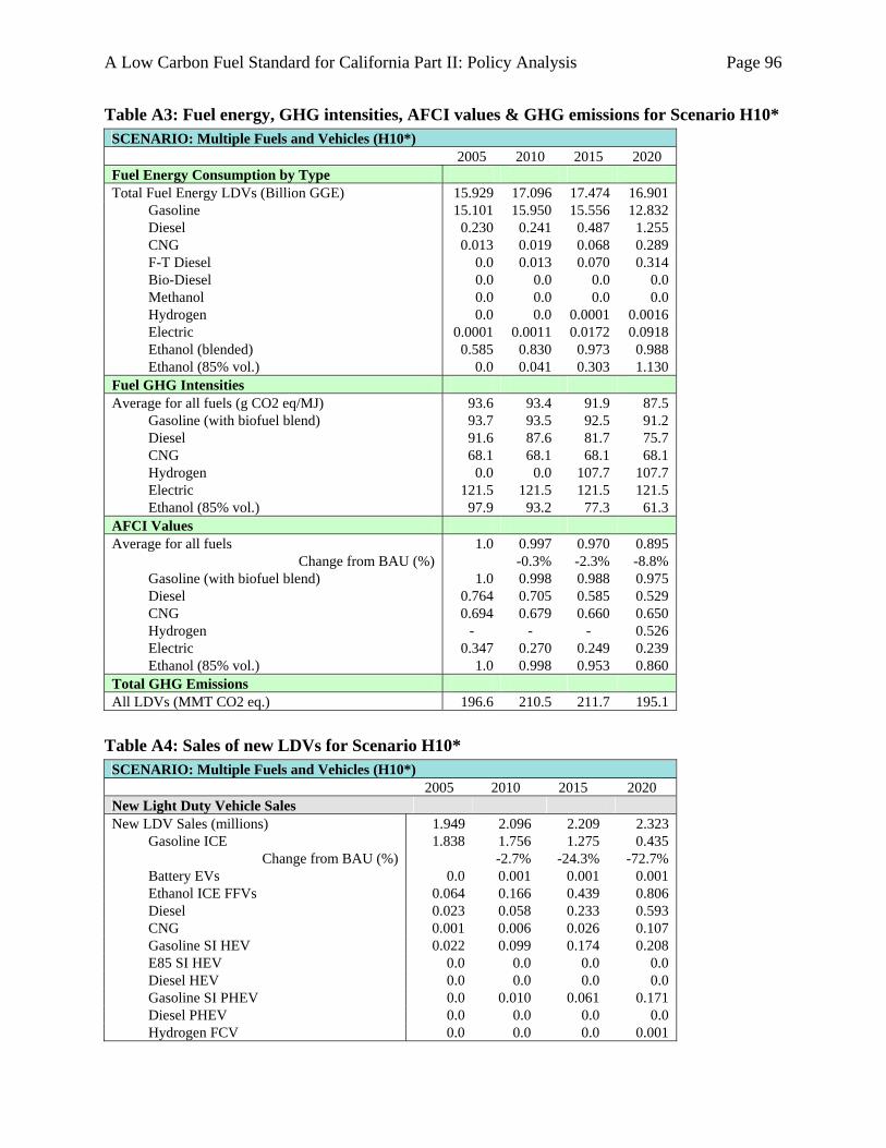
A Low Carbon Fuel Standard for California Part II: Policy Analysis Page 96
Table A3: Fuel energy, GHG intensities, AFCI values & GHG emissions for Scenario H10* SCENARIO: Multiple Fuels and Vehicles (H10*) 2005 2010 2015 2020 Fuel Energy Consumption by Type Total Fuel Energy LDVs (Billion GGE) 15.929 17.096 17.474 16.901 Gasoline 15.101 15.950 15.556 12.832 Diesel 0.230 0.241 0.487 1.255 CNG 0.013 0.019 0.068 0.289 F-T Diesel 0.0 0.013 0.070 0.314 Bio-Diesel 0.0 0.0 0.0 0.0 Methanol 0.0 0.0 0.0 0.0 Hydrogen 0.0 0.0 0.0001 0.0016 Electric 0.0001 0.0011 0.0172 0.0918 Ethanol (blended) 0.585 0.830 0.973 0.988 Ethanol (85% vol.) 0.0 0.041 0.303 1.130 Fuel GHG Intensities Average for all fuels (g CO2 eq/MJ) 93.6 93.4 91.9 87.5 Gasoline (with biofuel blend) 93.7 93.5 92.5 91.2 Diesel 91.6 87.6 81.7 75.7 CNG 68.1 68.1 68.1 68.1 Hydrogen 0.0 0.0 107.7 107.7 Electric 121.5 121.5 121.5 121.5 Ethanol (85% vol.) 97.9 93.2 77.3 61.3 AFCI Values Average for all fuels 1.0 0.997 0.970 0.895
Change from BAU (%) -0.3% -2.3% -8.8% Gasoline (with biofuel blend) 1.0 0.998 0.988 0.975 Diesel 0.764 0.705 0.585 0.529 CNG 0.694 0.679 0.660 0.650 Hydrogen - - - 0.526 Electric 0.347 0.270 0.249 0.239 Ethanol (85% vol.) 1.0 0.998 0.953 0.860 Total GHG Emissions All LDVs (MMT CO2 eq.) 196.6 210.5 211.7 195.1
Table A4: Sales of new LDVs for Scenario H10*
SCENARIO: Multiple Fuels and Vehicles (H10*) 2005 2010 2015 2020 New Light Duty Vehicle Sales New LDV Sales (millions) 1.949 2.096 2.209 2.323 Gasoline ICE 1.838 1.756 1.275 0.435
Change from BAU (%) -2.7% -24.3% -72.7% Battery EVs 0.0 0.001 0.001 0.001 Ethanol ICE FFVs 0.064 0.166 0.439 0.806 Diesel 0.023 0.058 0.233 0.593 CNG 0.001 0.006 0.026 0.107 Gasoline SI HEV 0.022 0.099 0.174 0.208 E85 SI HEV 0.0 0.0 0.0 0.0 Diesel HEV 0.0 0.0 0.0 0.0 Gasoline SI PHEV 0.0 0.010 0.061 0.171 Diesel PHEV 0.0 0.0 0.0 0.0 Hydrogen FCV 0.0 0.0 0.0 0.001

A Low Carbon Fuel Standard for California Part II: Policy Analysis Page 97
(This page is intentionally blank.)

A Low Carbon Fuel Standard for California Part II: Policy Analysis Page 98
Appendix B: Structure of the California Oil, Electricity, and Natural Gas Industries Organizational Structure of the California Petroleum Industry The oil industry can be divided into four sequential stages: exploration, production, refining, and distribution/sale of finished fuels. Some integrated oil companies participate in multiple stages of the petroleum production process, while others simply produce, refine, or market finished products. These production stages are detailed below. 1. Exploration
Because the California oil industry is mature, little oil exploration is performed in the state and few new fields have been found in recent decades (approximately 100 exploratory wells were drilled in state in 2005 (CDC-DOGGR 2006)). Remaining unexplored areas are largely off-limits to production (e.g. offshore areas). Exploratory wells drilled in 2005 were drilled largely by independent exploration companies, and no drilling was performed by the large integrated oil corporations (CDC-DOGGR 2006).
2. Production
Active oil production occurs from 209 oil fields, but the vast majority of production comes from the ten largest fields: in 2005, 192 out of 256 Mbbl total production came from the ten largest fields (CDC-DOGGR 2006). Oil production in California occurs from a large number of producing wells (approximately 50,000 operating wells (CEC 2007)), but about 25,000 of these wells are “stripper wells” with production of less than 10 bbl per day (CDC-DOGGR 2006). A large number of small companies operate these stripper wells (80% of production companies own 2 or fewer wells (CEC 2007)). Thus, while most production comes from large companies operating large oil fields, there are a significant number of small oil producers in the state. Oil in California has increasingly been produced from heavy oil resources over the last 50 years. Heavy oil production increased significantly in the 1960s with the implementation of steam injection into heavy oil fields. Heavy oil now accounts for approximately 70% of total California production, and thermal EOR operations result in incremental production (production above that which would have occurred without steam injection) of 100 Mbbl in 2005, or 40% of total state production (CDC-DOGGR, 2006). Production in California is largely electrified, with an average rate of consumption of 14 kWh per bbl (CEC 2007). Production of steam for heavy oil recovery through thermal EOR relies almost entirely on natural gas, with small amounts of coal consumed. Pumping operations in oil production consume about 1.5% of electricity produced in state (not including refining) (CEC 2007). Statewide capacity for co-production of electricity from thermal EOR operations totaled 2000 MW statewide in 2005, or about 4% of peak state demand.

A Low Carbon Fuel Standard for California Part II: Policy Analysis Page 99
3. Refining There are 21 refineries operating in the state of California (CEC 2007). They are concentrated in the urban areas of Southern and Northern California, with a few smaller refineries operating in Central California, mostly in the San Joaquin valley (Worrell and Galitsky 2004). These refineries process a mixture of in-state oil (40% in 2005), domestic imports (20% from Alaska), and foreign imports (40%) (CEC 2007). Oil is transported to refineries via pipeline from major production areas, or via pipelines from tanker offloading facilities. Thus, the coastal location of refineries is important in an era of increasing imports. California refineries are different, on average, from refineries in other parts of the United States for two reasons: they produce a higher-quality gasoline product (California reformulated gasoline) and they process a larger amount of heavy oil. Both of these differences would tend, on average, to increase the energetic demand of refining. Refining is energy intensive, consuming 15% of the electricity and 28% of the natural gas used by the manufacturing sector in California (CEC, 2007 #6836). Over time, the number of refineries operated in California has declined, while their average size has increased (Worrell and Galitsky 2004). Many refineries now process over 100,000 bbl/day. The remaining refineries in California are almost universally operated by large integrated corporations (e.g. Chevron-Texaco) or dedicated refining corporations (e.g. Valero). Exceptions include two smaller independently-owned refineries in Bakersfield (Worrell and Galitsky 2004).
4. Marketing and sales
Marketing and sale of finished petroleum products is occurs in over 10,000 fueling stations that have a variety of ownership schemes (WSPA 2007). Some are owned and operated by refiners or large integrated firms (e.g. Valero or Chevron-Texaco). Others are franchised or leased from larger firms by independent operators, and still others are owned and operated by independent business owners.
References CDC-DOGGR (2006). 2005 Annual Report of the State Oil & Gas Supervisor. Sacramento, CA,
California Department of Conservation: Division of Oil, Gas and Geothermal Resources. CEC. (2007). "Oil and petroleum in California." Retrieved 3-6-07, 2007, from
http://www.energy.ca.gov/oil/index.html. CEC. (2007). "Petroleum industry profile." Retrieved July 26, 2007, from
http://www.energy.ca.gov/pier/iaw/industry/petro.html. Worrell, E. and C. Galitsky (2004). Profile of the petroleum refining industry in California.
California Industries of the Future Program. Berkeley, CA, Energy Analysis Department, Lawrence Berkeley National Laboratory: 54.
WSPA. (2007). "California petroleum industry overview." Retrieved July 26, 2007, from http://wspa.org/issues/iff_cpio.htm.
Organizational Structure of Electric and Natural Gas Utilities in California The organizational structure of natural gas and electric utilities in California differs from that of traditional, competitive fuel distribution businesses in a variety of ways. Utilities in California

A Low Carbon Fuel Standard for California Part II: Policy Analysis Page 100
fall into two categories: Investor owned utilities (IOUs), which are regulated by the California Public Utilities Commission (CPUC), and municipal utilities, which are governed by local governing boards such as special district elected officials or city councils. The following describes how IOUs’ and municipal utilities’ behavior in the fuel marketplace is impacted by their organizational structure. 1. Electrical Utility Profits Not Linked To Sales Of Procured Energy IOUs
California IOUs provide what is called “cost based service” to their customers, and do not profit from sales of procured energy. Only the actual cost of the commodity is recovered when an IOU procures gas or electricity from third parties for delivery to its customers. The cost recovery is “at cost” and no profit component is included. Therefore, California IOUs do not have a direct profit incentive to increase natural gas or electricity sales. An IOU’s investors do have an opportunity to increase earnings through investments in generation, transmission and distribution infrastructure in the event that additional capacity is required to meet additional peak demands.36 To cover a utility’s fixed costs, a base revenue requirement is established for each utility by the CPUC based on reasonable projected costs, plus a rate-of-return for capital investments in facilities that serve customers. A utility essentially receives this revenue requirement regardless of the number of kilowatt-hours or therms sold. Utility profit risk is therefore based on controlling costs and capital project completion, not sales of energy.37
Utilities are interested in natural gas and electric transportation for a variety of other reasons, such as: (1) environmental stewardship, (2) compliance with the Energy Policy Act of 1992’s alternate fuel fleet requirements and other laws and regulations that affect California utilities and their customers’ fleet decisions, as well as (3) the ability of natural gas and electric vehicles to contribute to the more efficient use of existing utility infrastructure.
Except for a brief period of deregulation, ratemaking for California IOUs has, for over 20 years, been subject to "de-coupling" of sales volumes from revenues to ensure the volume of energy sales is separated from profit motivations.38 Under the "de-coupling" ratemaking principle, utility revenues are subject to "true-up" after each ratemaking period to adjust for any revenues that are attributable to higher or lower sales of electricity or gas. Under the “true-up", increases in energy consumption by utility customers do not result in greater cost recovery (or increased earnings) by the utility. Decreases in consumption (and associated revenue) are treated similarly. Under this design, utilities earn no added profit by increasing sales; they simply recover their cost of service. California’s leadership on this de-coupling policy removed a previous disincentive to achieving reduced consumption through energy efficiency, which is the first priority resource under the State’s Energy Action Plan because it is the most cost-effective resource option.
36 Infrastructure investments needed to meet electric vehicle demand are expected to be very minor, if any, and for
natural gas, relatively minor, at least in the near and medium term. 37 It should be noted that a portion of PG&E's local transmission, storage and backbone revenues are subject to
throughput risk (i.e. have revenues and profits tied to sales) for deliveries of natural gas. 38 Please see the following CPUC document which describes “de-coupling” in relatively simple terms:
www.cpuc.ca.gov/eeworkshop/cpuc-new/design/docs/deccouplinglowres.pdf

A Low Carbon Fuel Standard for California Part II: Policy Analysis Page 101
Municipal Utilities. Municipal utilities are customer owned and provide electricity as a cost-recovery based service similar to the IOUs under the decoupling structure. Whereas an IOU’s investors have the opportunity to earn a rate of return on the IOU’s capital investments, municipal utilities finance capital projects for themselves and do not generate any rate of return. Municipal utilities are motivated to keep rates as low as possible in meeting customer needs because of their customers’ access to publicly elected, local board members.
2. Utilities Are Subject To Regulations Designed to Reduce GHG Emissions California utilities are currently subject to rules designed to reduce the carbon footprint of the electricity they sell. For example, the Renewable Portfolio Standard (RPS) requires California IOUs to have contracts for 20% of their deliveries to be renewable by 2010.39 The governing boards of local publicly-owned electric utilities are responsible for implementing and enforcing an RPS that recognizes the intent of the Legislature to encourage renewable resources.405
In addition, new, long-term electricity contracts entered into by load serving entities, including municipal utilities, are required by Senate Bill 1368 to deliver electricity that is at least as low-carbon as that from a natural gas combined-cycle combustion turbine (NG CCCT). Newer NG CCCT’s are less than half as carbon intensive as a new supercritical coal power plant.41
3. Utilities Have an Obligation to Serve
In general, California utilities must serve any customer who requests electric or natural gas service, follows service connection rules and is not overdue on payments. In contrast, competitively organized transportation fuel providers can choose to reduce service or exit the California marketplace if regulatory burdens become uneconomic, an option not shared by utilities.
4. Interaction between Regulated and Unregulated Businesses of IOUs The CPUC has developed affiliate rules42 primarily intended to ensure that affiliates and their customers do not receive an unfair advantage over other market participants because of their affiliation with an IOU and/or its holding company.
39 RPS eligible renewable energy includes biomass, geothermal, solar, wind, and small hydroelectric projects.
Utilities also have carbon-neutral resources that are not counted towards RPS goals, including large hydroelectric projects and nuclear energy.
40 Per SB 1368 legislative counsel’s digest. TIAX LLC, “Full Fuel Cycle Assessment – Well to Tank Emissions and Energy Consumption,” CEC Report CEC-600-2007-003, June 2007, Figure 7-20, GHG Emissions for Electricity.
41 Some regulated IOUs have unregulated lines of business (affiliates) that are not subject to the same rights and responsibilities as their regulated counterparts. However, only the regulated utility companies can provide retail service of electricity and natural gas.
42 The latest CPUC decision adopting updated affiliate rules can be found here: http://www.cpuc.ca.gov/PUBLISHED/FINAL_DECISION/ 63087.htm ; http://www.cpuc.ca.gov/PUBLISHED/Graphics/63089.PDF

A Low Carbon Fuel Standard for California Part II: Policy Analysis Page 102
Appendix C: Simple Calculation of Indirect Land Use Change Effects
originaldata unit source
calculateddata unit
total land area of earth 149 million km2 CIA Factbook 1.5E+14 m2fraction land in crops 0.18 ratio CIA Factbook 1.8E-01 ratiototal cropland area 2.7E+13 m2crop conversion carbon emissions Houghton 1999 (data for 1980's) 1.3E+15 g C /yrcarbon emissions per cropland area 4.8E+01 g C / m2CO2e per cropland area 1.8E+02 g CO2e / m2CO2e per cropland area 1.8E+06 g CO2e / haCO2e per cropland area 7.2E+05 g CO2e / acre
fraction of cropland in all biofuels 2.9E-03 ratiototal energy in biofuels 7.7E+11 MJ /yrcarbon emissions per avg unit fuel 4.9E+00 g C / MJ CO2e per avg unit fuel 18 g CO2e / MJ
US Corn Ethanol (Average)fuel production 4885 million gal ethanolrfa.org (2006) 4.0E+11 MJ / yrcrop yield per land area 150 bu / acre NCGA World of Corn (Avg 2003-2006) 9.4E-01 kg / m2fuel yield per crop 2.71 gal / bu GREET 1.7 8.7E+00 MJ / kgfuel yield per land area 8.2E+00 MJ / m2land area per unit fuel 1.2E-01 m2 / MJland area in crop 4.9E+10 m2CO2e per unit fuel 22 g CO2e / MJ
Brazilian Sugar Ethanol (Best Case)fuel production 4491 million gal ethanolrfa.org (2006) 3.7E+11 MJ / yrcrop yield per land area 68700 kg / ha Macedo et al 2004 6.9E+00 kg / m2fuel yield per crop 0.086 L /kg Macedo et al 2004 1.8E+00 MJ / kgcrop ethanol yield per land area 1.3E+01 MJ / m2land area per unit fuel 8.0E-02 m2 / MJland area in crop 2.9E+10 m2CO2e per unit fuel 14 g CO2e / MJ
Switchgrass Ethanol (Projected)fuel production 0.0E+00 MJ / yrcrop yield per land area 13450 kg / ha GREET (via EBAMM Cellulosic) 1.3E+00 kg / m2fuel yield per crop 0.38 L /kg GREET (via EBAMM Cellulosic) 8.1E+00 MJ / kgfuel yield per land area 1.1E+01 MJ / m2land area per unit fuel 9.2E-02 m2 / MJland area in crop 0.0E+00 m2CO2e per unit fuel 16 g CO2e / MJ

A Low Carbon Fuel Standard for California Part II: Policy Analysis Page 103
originaldata unit source
calculateddata unit
Soybean Biodiesel (Average)fuel production 0.0E+00 MJ / yrcrop yield per land area 43 bu/ac NASS 2005 Ag Statistics 2.9E-01 kg / m2oil yield per crop 0.17 kg / kg Sheehan (NREL) et al 1998 1.7E-01 kg / kgfuel yield per oil 1.04 kg / kg Sheehan (NREL) et al 1998 3.8E+01 MJ / kgfuel yield per land area 1.8E+00 MJ / m2land area per unit fuel 5.4E-01 m2 / MJland area in crop 0.0E+00 m2CO2e per unit fuel 96 g CO2e / MJ
Palm Oil Biodiesel (Average)fuel production 0.0E+00 MJ / yrcrop yield per land area 20000 kg of ffb/ha http://www.fao.org/DOCREP/005/Y43 2.0E+00 kg / m2oil yield per crop 0.25 kg / kg of ffb http://www.fao.org/DOCREP/005/Y43 2.5E-01 kg / kgfuel yield per oil 1.04 kg / kg Sheehan (NREL) et al 1998 3.7E+01 MJ / kgfuel yield per land area 1.8E+01 MJ / m2land area per unit fuel 5.4E-02 m2 / MJland area in crop 0.0E+00 m2CO2e per unit fuel 10 g CO2e / MJ
Conversion factors Value Source g CO2e / MJacre / ha 2.5 US Corn Ethanol 22Joules per Btu 1055.0 Brazilian Sugar Ethanol 14Btu per gallon of gasoline 115400.0 US Switchgrass Ethanol 16Energy content of ethanol (MJ/L) 21.2 US Soybean Biodiesel 96kg/bu corn 25.4 Palm Oil Biodiesel 10kg/bu soy 27.2L/gal 3.9GGE/gallon EtOH 0.7lbs/ kg 2.2Short Tons / Metric Ton 0.9MJ / L Gasoline (LHV) 31.5MJ / L Diesel (LHV) 37.8MJ / kg Biodiesel 37.0NREL) et al 1998