Meteor radar wind and temperature measurements over Collm (51.3°N, 13°E) and comparison with co-located LF drift measurements during autumn 2004 Ch. Jacobi, D. Kürschner, K. Fröhlich, K. Arnold, G. Tetzlaff Zusammenfassung Seit Juli 2004 wird an der Außenstelle Collm der Universität Leipzig kontinuierlich ein Mete-orradar zur Messung des Windes und der Temperatur im Höhenbereich 80-100 km betrieben. Die Messungen dienen der Überwachung der Dynamik der Mesopausenregion, und ihrer Än-derungen auf Zeitskalen von Tagen und Jahren. Erste Ergebnisse vom Herbst 2004 werden dargestellt, verglichen mit den ebenfalls am Collm durchgeführten Langewellenreflexions-windmessungen. Die Ergebnisse zeigen, dass die vertikale Struktur des Windsystems und die Variationen von Tag zu Tag qualitativ übereinstimmen. Die mit dem Meteorradar gemessenen Gezeitenamplituden sind jedoch systematisch größer als diejenigen, die mit dem Langewel-lenverfahren gemessen wurden. Abstract Since July 2004 winds and temperatures in the height range 80-100 km are measured using a meteor radar. The data are used to monitor upper middle atmosphere dynamics and dynamical changes at time scales from days to years. First results obtained during the autumn transition of the mesosphere/lower thermosphere wind field 2004 are presented, as well as a comparison with the low-frequency winds measured at Collm. The results show a good agreement of the overall wind structure and the day-to-day variations of wind parameters. However, the tidal amplitudes measured by meteor radar are systematically larger than those measured with the low-frequency method. 1 Introduction Over the last three decades, ground-based instruments, and among them especially radars, have offered powerful insights into the dynamical structure of the mesosphere/lower thermo-sphere (MLT) region at a height range of about 80-100 km. However, a major limitation in such work to date has been the very small number of long-term continuous MLT-region wind measurements. One of the longest homogeneous MLT wind time series available worldwide has been measured at Collm Observatory using low-frequency (LF) radio waves. The data has been analysed with respect to long-term variations, and are also contributed to empirical mod-els of the MLT (Portnyagin and Solovjova, 1998, Portnyagin et al., 2004). The measurements are carried out according to the LF spaced receiver method, which makes the time series a unique one. This, however, bears the potential of undetected biases when the data are used in combination with those measured with other methods, e.g., to detect wavenumbers of plane-tary waves (Pancheva et al., 2004). Although some comparison of LF winds with medium frequency (MF; Hoffmann et al., 1990; Singer et al., 2000) and meteor radar (MR; Lysenko et al., 1972) winds has been performed, these comparisons had to use data from somewhat dif-ferent measuring volumes, and partly also times of day and heights. They are therefore of limited significance.

In summary, it has proved to become favourable to complete the Collm LF measurements by a standard wind measuring method, and operate the two methods simultaneously for a long time interval of at least one year in order to detect possible systematic differences of the re-sults obtained with both methods. To this aim, in summer 2004 a commercial MR system has been installed at Collm and is continuously operated since then. This paper presents some first result of these measurements, and comparison with LF wind data during autumn 2004. Since the potential errors of both MR and LF measurements are dependent on the seasonal peculi-arities (as mean wind and tidal wind gradients, meteor flux rates, length of the day, wind field variability, etc.), the results thus far have to be considered as preliminary. Nevertheless, a first impression on the potentials of both methods, and their limitations, may be provided by these comparisons. 2 Radar description and data analysis 2.1 Specific details of the radar The meteor radar is a commercially produced VHF system manufactured under the brand name SKiYMET. The radar operates with a frequency of 32.6 MHz and a peak power of 6 kW. The transmitter produces short pulses (~13 µs) at a pulse repetition frequency of 2144 Hz in the standard mode of operation. The radar operates in an “all-sky” configuration with the radiated power from a vertically pointing 3-element Yagi antenna (left part of Figure 1). Five individual 2-element Yagi receiving antennas with horizontal distance of 2 or 2.5 wave-lengths, respectively, forming a cross are configured to act as an interferometer. The interfer-ometer is situated near the Collm Observatory main building at 51.3°N, 13°E at the slope of the Collm mound about 230 m asl, with an interferometer plane slope of 7°. The transmitter and receiver are housed in a shack (right part of Figure 1) about three wavelengths away from the transmit antenna. The measured data are collected on a PC in the shack, where on-line standard data evaluation is performed also. These data, as well as the raw data, are transferred to a workstation at the Institute for Meteorology in Leipzig once a day. The radar continually collected data since

Figure 1: Left: Transmit antenna. In the foreground the trench to carry the feeder cable is still open. Right: Transmitter (right rack) and receiver unit (left rack) installed on a table.

July 2004. In Europe, other SKiYMET meteor radars are operated in Kühlungsborn, Ger-many, Andenes, Norway (Singer et al., 2004), and Esrange, Sweden (Mitchell et al., 2002).

2.2 Wind measurements The wind measurement principle is the detection of the Doppler shift of the reflected VHF radio waves from ionised meteor trails, which delivers radial wind velocity along the line of sight of the VHF radio wave. The interferometer is used to detect azimuth and elevation angle from phase comparisons of individual receiver antenna pairs. Together with the range meas-urements the meteor trail position is detected. The raw data collected consist of azimuth and elevation angle, wind velocity along the line of sight, meteor height, and additionally decay time for each single meteor trail. The data collection procedure is also described in detail by Hocking et al. (2001). The meteor trail reflection heights are varying roughly between 75 and 110 km, with a maxi-mum around 90 km. In standard configuration, the data are binned in 6 different height gates centred at 82, 85, 88, 91, 94, and 98 km. Individual winds calculated from the meteors are collected to form hourly mean values using a least squares fit of the horizontal wind compo-nents to the raw data under the assumption that vertical winds are small (Hocking et al., 2001). An outlier rejection is added. An example of hourly zonal and meridional winds is pre-sented in Figure 2. 24-hourly smoothed wind values are also added. The strongest signal that is visible at time scales within one day is the semidiurnal tide (SDT). The 24-hr smoothed winds show a distinct day-to-day variability, which is the signal of the quasi-two-day wave (QTDW), a common feature in the summer MLT at midlatitudes (Pancheva et al., 2004). Comparison of the zonal and meridional wind variability shows that both the SDT and

Figure 2: Example of hourly man winds measured by the Collm MR in the height gate centred at 91 km. 24-hr running averages are added as thick lines.

QTDW meridional phases head the zonal ones by 90° (clockwise circularly polarized wind components), which is in accordance with linear theory. The meteor radar wind measurements are intended to complete the existing wind measure-ments at Collm. These measurements base on the reflection of LF radio waves from 3 com-mercial transmitters (177, 225, and 270 kHz) at oblique incidence with transmitter distances between 160 and 460 km. The data are interpreted using the spaced receiver method and are analysed with an algorithmised form of the similar fade method (Kürschner, 1975, 1981; Kürschner and Schminder, 1980). The individual wind measurements are also combined to mean values using a weighting function essentially based on estimates of the chaotic velocity. The reflection height is detected through phase comparisons of the ground wave and the sky wave in a small side-band frequency range near 1.8 kHz (Kürschner et al., 1987). 2.3 Temperature estimation from MR measurements In addition to the wind measurements using MR, the decay time of the signal is detected from so-called underdense meteor trails, i.e. from those trails whose reflectivity is determined by their electron density. The decay time τ10 is the time, after which the signal falls to 10% due to diffusion, so that daily mean temperatures can be obtained from the ambipolar diffusion coef-ficients Da that are estimated from τ10:

λπ

−= tD16

expAA 2a

2

0 , (1)

with A as the signal amplitude, λ as the radar wavelength and t as time. Thus, τ10 can be esti-mated from the amplitude curve to yield:

10ln16

D10

2

2

a τπλ= . (2)

The diffusion coefficient is proportional to the ratio of temperature squared and pressure (Jones and Jones, 1990):

pTKD

2

a = , (3)

with K as a constant. Knowledge of pressure, e.g. from the CIRA or MSIS model, thus en-ables one to calculate temperature (Hocking, 1997). However, using pressures from empirical models potentially causes errors if the models are incorrect. Therefore a method described by Hocking (1999) is used to derive absolute temperatures under the assumption that the relative vertical temperature gradient α = (1/T⋅)dT/dz is constant around the height of the maximum meteor flux rate near 90 km. We introduce a vertical coordinate z with z = 0 at 90 km altitude, introduce T = T0 (1- αz) in Eq. (3), and apply a pressure decay with scale height

∫⋅==

−z

0H

´dz

e)0z(pp , where H = mg/kT with k as Boltzmann´s constant and m, g as the mean molecular mass and acceleration due to gravity at 90 km. Then Eq. (3) may be written as:

( ) ( ) .e)0z(pz1KTD

z

0 0´dz

´z1kTmg

20a

∫=α−= α− (4)

Taking the logarithm of Eq. (4) and differentiating with respect to z, one obtains an equation for the temperature in dependence of the diffusion coefficient change with height for z = 0:

,kTmg

TdzdT2

dzDlnd

00

a +−= (5)

which may be solved for T0. This method still requires the assumption of the temperature gra-dient dT/dz that is taken from an empirical model. More details can be found in Hocking (1999). Temperatures estimated with this method has been presented by Hocking et al. (2004) and Singer et al. (2004), also showing validation with rocket and ground-based optical meth-ods. Temperatures measured during autumn 2004 at Collm using Eq. (5) will be shown in section 4. 3 MLT wind comparison during Autumn 2004 In this paper we focus on the analysis of data gathered during September and October 2004. This includes the late summer situation, and the autumn transition, connected with a mean wind reversal – sometimes called “autumn anomaly” – in the upper MLT. We analysed the MR wind data together with the LF winds, using the same procedures. 3.1 Mean monthly winds Monthly mean zonal and meridional winds for each time of day are shown in Figure 3. In-cluded are LF winds, separately for each of the three frequencies used and the weighted means, as well as all measured MR hourly means data between 82 and 98 km. No height separation is applied here, therefore the MR winds may be attributed to the height of maxi-mum MR reflections that is around 90 km. Also shown in Figure 3 are the monthly mean LF reflection heights. The comparison is not shown as a scatter plot, because the diurnal wind variations can be shown better using time series. The major variation at time scales up to one day is the SDT, with maxima in the morning and early evening for the zonal component, while the meridional component heads the zonal one by 3 hours. The tidal amplitudes are much larger in September than in October, which is in accordance with climatological values (e.g. Jacobi et a., 1999; Manson et al., 2002). The shift of the phase, which is usually expressed as the time of westward wind maximum, to later val-ues in October represents the seasonal variation from summer to winter conditions. The differences between the radar and LF winds are small; some larger differences are seen during the morning and evening hours, owing to the comparatively low LF reflection heights then. The comparison shows that both MR and LF mean winds are in satisfactory correspon-dence in measuring wind variations at time scales within one day.

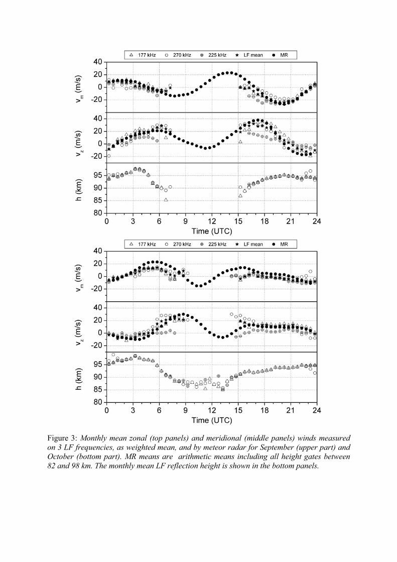
Figure 3: Monthly mean zonal (top panels) and meridional (middle panels) winds measured on 3 LF frequencies, as weighted mean, and by meteor radar for September (upper part) and October (bottom part). MR means are arithmetic means including all height gates between 82 and 98 km. The monthly mean LF reflection height is shown in the bottom panels.

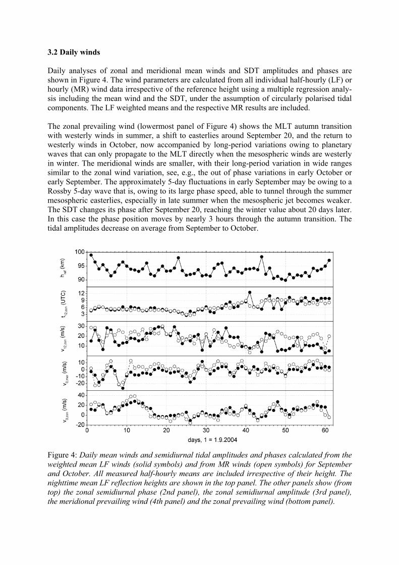
3.2 Daily winds Daily analyses of zonal and meridional mean winds and SDT amplitudes and phases are shown in Figure 4. The wind parameters are calculated from all individual half-hourly (LF) or hourly (MR) wind data irrespective of the reference height using a multiple regression analy-sis including the mean wind and the SDT, under the assumption of circularly polarised tidal components. The LF weighted means and the respective MR results are included. The zonal prevailing wind (lowermost panel of Figure 4) shows the MLT autumn transition with westerly winds in summer, a shift to easterlies around September 20, and the return to westerly winds in October, now accompanied by long-period variations owing to planetary waves that can only propagate to the MLT directly when the mesospheric winds are westerly in winter. The meridional winds are smaller, with their long-period variation in wide ranges similar to the zonal wind variation, see, e.g., the out of phase variations in early October or early September. The approximately 5-day fluctuations in early September may be owing to a Rossby 5-day wave that is, owing to its large phase speed, able to tunnel through the summer mesospheric easterlies, especially in late summer when the mesospheric jet becomes weaker. The SDT changes its phase after September 20, reaching the winter value about 20 days later. In this case the phase position moves by nearly 3 hours through the autumn transition. The tidal amplitudes decrease on average from September to October.

Figure 4: Daily mean winds and semidiurnal tidal amplitudes and phases calculated from the weighted mean LF winds (solid symbols) and from MR winds (open symbols) for September and October. All measured half-hourly means are included irrespective of their height. The nighttime mean LF reflection heights are shown in the top panel. The other panels show (from top) the zonal semidiurnal phase (2nd panel), the zonal semidiurnal amplitude (3rd panel), the meridional prevailing wind (4th panel) and the zonal prevailing wind (bottom panel).

The prevailing MR and LF winds agree very well, which is both the case with the day-to-day variations and with the absolute value (with only a small bias in the meridional component). The tidal phases also agree, apart from some fluctuations of the LF phase in October which is averaged out in the MR winds probably owing to the larger measuring density and the com-plete coverage of the diurnal cycle, in the presence of increased tidal phase gradients toward winter months. However, the SDT amplitudes as measured by MR are sometimes considera-bly larger than those evaluated from LF drifts. This is a phenomenon often visible in connec-tion with comparisons between MR measurements and closely spaced measurements. One reason for the discrepancy may be in some cases the incomplete daily coverage by LF meas-urements (see Figure 3), but possible effects of VHF reflections not connected with meteor at greater heights (e.g. during sporadic E conditions) cannot be excluded also. Elucidation of the reasons of the differences requires fundamental methodical investigations and further analysis using a larger dataset taken during different seasons. 3.3 Wind profile structure Analysing mean winds without taking into account the height information does not exploit the potentials of both methods. Wind profiles can be calculated from the individual LF half-monthly means using a multiple regression analysis with height-dependent coefficients (Groves, 1959; Kürschner and Schminder, 1986). The spectral selectivity of the separation of prevailing and tidal wind can be improved through fitting the measured values for the two horizontal wind components as a vector, assuming clockwise circularly polarized tidal wind components (Kürschner, 1991). September mean profiles of the prevailing winds as well as the SDT amplitudes and phases are shown in Figure 5. The profiles measured by MR are also added. The MR data have been analysed in the same manner as the LF winds, although in principle the analysis of single height gates here can be performed also. The corresponding profiles for October are shown in Figure 6. In September, both prevailing winds and tidal amplitudes measured by the two systems are of the same order of magnitude. To give an impression of the intermonthly variability, two pro-files independently calculated for the first and second half of this month are added in Figure 5. Generally, during September the wind shift from summer to autumn conditions appears, which leads to strong differences between the first and second half of this month. Thus, the differences between LF and MR results are smaller than the wind variations themselves. For October, however, the picture looks less conclusive. While meridional prevailing winds and SDT phases agree reasonably well, the MR zonal prevailing wind system is shifted down-wards, as the SDT amplitudes do also. Inspection of the time series in Figure 4 shows that intermittently during the second half of October the MR amplitudes grow larger than the LF ones, while during other time intervals this is not the case. There are several possible reasons for the measured differences. The measured LF heights above 95 km are affected by group retardation so that the measured heights, assuming wave propagation with the speed of light, are too high. When these data are included in a regression analysis, this may influence the entire LF wind profile, which should be shifted a bit down-ward. However, this effect is smaller than the differences seen in Figure 6. Another possible source of difference may be incomplete coverage of the day with half-hourly wind values us-ing the LF method. During daylight hours the reflection heights are low, and measurements are sparse. This may have an effect on the decomposition into mean winds and tides, i.e. part of the tidal signature may contribute to the mean winds, or vice versa. Another possible source of error may be disturbed lower ionospheric conditions that may affect VHF reflection.

Figure 5: September mean profiles of zonal prevailing wind (upper left panel), meridional prevailing wind (upper right panel), zonal semidiurnal phase (lower left panel) and zonal semidiurnal amplitude (lower right panel) by MR and LF drifts. In addition, half-monthly radar profiles are also added. Profiles are calculated by a multiple regression analysis with quadratically height dependent coefficients.

Figure 6: October mean profiles of zonal prevailing wind (upper left panel), meridional prevailing wind (upper right panel), zonal semidiurnal phase (lower left panel) and zonal semidiurnal amplitude (lower right panel) by MR and LF drifts. Profiles are calculated by a multiple regression analysis with quadratically height dependent coefficients.

0 3 6 9 12 15 18 21 24-30

-20

-10

0

10

20

30

40

50

Radar 82+85 km Fitted line LF < 92 km

Time (UT)

mon

thly

mea

n zo

nal w

ind

(m/s

)

0 3 6 9 12 15 18 21 24

-30

-20

-10

0

10

20

30

40

Time (UT)

mon

thly

mea

n m

erid

iona

l win

d (m

/s)

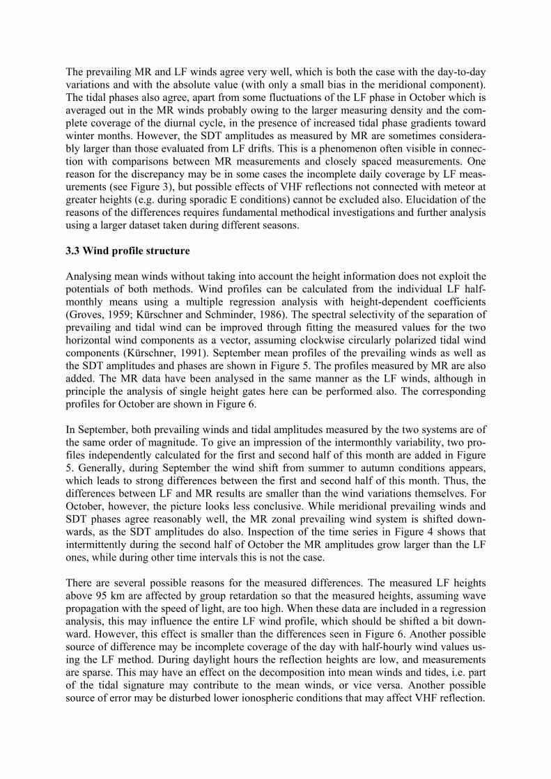
Figure 7: September 2004 monthly mean zonal (left panel) and meridional (right panel) winds measured by radar at height gates 82 and 85 km, and mean LF winds for height below 92 km. The results of a multiple regression including the mean wind, semidiurnal and diurnal tide applied to the radar data is added as a fitted line.

0 3 6 9 12 15 18 21 24

-30

-20

-10

0

10

20

30

40

50

Time (UT)

Radar 94+98 km Fitted line LF > 92 km

mon

thly

mea

n zo

nal w

ind

(m/s

)

0 3 6 9 12 15 18 21 24-40

-30

-20

-10

0

10

20

30

40

Time (UT)

mon

thly

mea

n m

erid

iona

l win

d (m

/s)

Figure 8: As in Figure 7, but for height gates 94 and 98 km, and mean LF winds for heights above 92 km. To investigate the differences in height structure further, in Figure 7 the monthly mean MR winds calculated from 2 low-level height ranges are shown together with LF results for the upper half of the measuring volume. The corresponding results for high levels are shown in Figure 8. Also added in the figures are the results of a MR wind decomposition into mean wind, diurnal tide (DT), and SDT. It can be seen that the SDT and DT well describes the wind field, the residuals, as shown in Figure 9, are smaller than 10 ms-1. However, it can be seen that the residual structure has a distinct 8-hourly component, which is probably related to the terdiurnal tide (TDT). The TDT is generally believed to result from non-linear interaction between the diurnal and semidiurnal tide (Glass and Fellous, 1975; Teitelbaum et al., 1989). A global analysis of the TDT from UARS HRDI satellite wind measurements has been pre-sented by Smith (2000), revealing zonal amplitudes of about 10 ms-1 in correspondence with results by Glass and Fellous (1975), and meridional amplitudes being smaller. While the zonal amplitudes shown in Figure 9 are somewhat smaller, the relation between zonal and meridional amplitudes qualitative corresponds to the literature results. We may conclude that the MR measurements also provide information about the TDT, which will be included in further analyses.

0 3 6 9 12 15 18 21 24-10

-5

0

5

10

-10

-5

0

5

10

Time (UT)

zona

l (m

/s)

82+85 km 88+91 km 94+98 km

mer

idio

nal (

m/s

)

Figure 9: Meteor radar residuals of the fitted lines as shown in Figure 7 and Figure 8, for three heights. The main contribution is due to the 8-hour tide. From the left panels of Figure 7 and Figure 8 it can be seen that the differences between LF and MR zonal means are height-dependent, and reflect the smaller (larger) MR winds at lower (upper) layers as visible in Figure 5. However, these differences are not independent of the time of day, but are found especially during early night. This may indicate that there may be an influence of LF mean height changes on the results, which has to be investigated further. 4 Mesopause region temperatures MR temperatures are calculated once a day from the vertical diffusion coefficient gradient using Eq. (4). The temperatures are attributed to the height of maximum measuring density at 90 km. The temperature time series is shown in the left panel of Figure 10, together with the MR wind values at 91 km. The overall temperature structure shows the seasonal cycle, with changes from the cold summer mesopause to the winter situation in September. The cold summer temperatures are accompanied by southward (negative) meridional winds which are owing to the mesospheric easterlies that again are accompanied by westerlies near the mesopause. The QTDW in August is visible in both wind components, with a tendency to-wards larger amplitudes in the meridional component. The temperature increase starts around August 15 and is connected with the zonal wind de-crease that starts at exactly the same time. The change towards the autumn anomaly begins around September 5, and maximum westward zonal winds are measured near September 25. This time interval is closely related to the transition interval from southward summer to near-zero winter meridional winds, and also marks the time interval of temperature increase. This behaviour well reflects the dynamical forcing of MLT temperatures through the meridional circulation, which is again steered by the mesospheric zonal wind.

Figure 10: Top panel: daily mean temperatures (open circles, upper right axis) and 24-hr smoothed zonal winds (upper part, left axis) and meridional (lower part, lower right axis) measured by MR at 91 km (solid lines). Bottom panel: amplitude spectra of MR zonal winds at 91 km (solid line with open circles), LF zonal winds on 177 kHz (dotted line with solid cir-cles) and MR temperatures (dashed line). Data are taken from Sept. 20 through Nov. 18, 2004 (days 50-110).

A direct connection between wind and temperature variability in August is not visible, since the QTDW structure cannot be inferred from daily temperatures. However, starting with the autumn westward zonal wind maximum around September 25 a clear long-period oscillation is visible in both wind components, which also seen in the temperatures. Spectra of tempera-tures and zonal winds (each using one data point per day) are shown in the lower panel of Figure 10 after removing a quadratic fit from the data. For comparison, the LF wind spectra taken from the measurements on 177 kHz are also added. The day-to-day variability includes peaks near 10 and 5 days, which may be attributed to the corresponding Rossby waves which are able to directly propagate to the MLT as long as the mesospheric zonal winds are east-ward. Largely, the wind and temperature spectra agree, especially regarding the 10-day oscil-lation, however, some wind variability is visible that is not at all reflected in temperatures. Note that the MR and LF spectra agree excellently in the period interval 5-12 days. For higher frequencies (with periods around 2 days), some additional day-to-day variability is seen in the LF winds, which is probably due to the possible shift of reflection heights from day to day and the incomplete coverage of the diurnal cycle in the presence of a diurnal tide. The 20-day peak (around 0.05 1/days) visible in LF winds is probably owing to potential changes of mean nighttime LF heights. 5. Conclusions and outlook Comparison of LF and MR winds show that the overall wind structure during the autumn transition ais well captured by both systems. The overall mean winds, irrespective of height, agree well (Figure 3), while the day-to-day variability shows extremely good correspondence (Figure 4 and Figure 10). This in particular is the case with the summer-winter transition, dates of maximum/minimum winds, and wave structures in the Rossby wave period range. Furthermore, the daily mean temperatures well reflect the seasonal and wave structures ex-actly as they are predicted by theory. We may conclude that the MR measurements are excel-lently suited to measure seasonal and long-period MLT wind variations. To conclude further, however, some open points remain. The gravest one concerns the differ-ences of the height profiles, which may partly be attributed to the small and inhomogeneously distributed LF measuring density concerning height and time. The second point include the larger MR SDT amplitudes compared to LF ones, which require careful analysis in a more comprehensive validation study. As can be seen from the analyses without respect to height information (see Figure 2), the SDT differences may partly also be due to a height error of the LF measuring system. A long-term analysis study with more detailed comparisons will be performed to clarify this points. Furthermore, it has to be kept in mind that, notwithstanding the collocated measuring devices, the wind information of the LF and MR is gathered from very different MLT measuring volumes. While the MR measures winds are taken essentially from a circle around Collm, the LF winds are collected at 3 relatively well defined reflection points North or East of Collm, and the measuring volumes only partly overlap. Further analy-ses will thus include the comparison of MR subvolumes with the LF winds to check whether the spatial difference have an influence on the mean winds. To summarise, it may be stated that with both methods the peculiarities of the MLT wind system can be measured, but systematic differences do occur. Since the LF spaced receiver method is the more indirect one of both, the MR results appear to be the more reliable ones. However, a final proof of this hypothesis is still required, before a possible reanalysis of the earlier LF wind data may be performed.

Acknowledgements This study was partly supported by INTAS under grant 03-51-5380. References Glass, M., and J.J. Fellous, 1975: The eight-hourly (ter-diurnal) component of atmospheric

tides, Space Res., 15, 191-197. Groves, G.V., 1959: A theory for determining upper-atmosphere winds from radio observa-

tions on meteor trails, J. Atmos. Terr. Phys., 16, 344-356. Hocking, W.K., 1999: Temperatures using radar-meteor decay times, Geophys. Res. Lett., 26,

3297-3300. Hocking, W.K., T. Thayaparan, and J. Jones, 1997: Meteor decay times and their use in de-

termining a diagnostic mesospheric temperature-pressure parameter: methodology and one year of data, Geophy. Res. Lett., 24, 2977-2980.

Hocking, W.K., B. Fuller, and B. Vandepeer, 2001: Real-time determination of meteor-re-lated parameters utilizing modern digital technology, J. Atmos. Solar-Terr. Phys., 63, 155-169.

Hocking, W.K., W. Singer, J. Bremer, N.J. Mitchell, P. Batista, B. Clemesha, and M. Donner, 2004: Meteor radar temperatures at multiple sites derived with SKiYMET radars and compared to OH, rocket and lidar measurements, J. Atmos. Solar-Terr. Phys., 66, 585-593, doi:10.1016/j.jastp.2004.01.011.

Hoffmann, P., W. Singer, D. Keuer, R. Schminder, and D. Kürschner, 1990: Partial reflection drift measurements in the lower ionosphere over Juliusruh during winter and spring 1989 and comparison with other wind observations, Z. Meteorol., 40, 405-412.

Jacobi, Ch., Yu.I. Portnyagin, T.V. Solovjova, P. Hoffmann, W. Singer, A.N. Fahrutdinova, R.A. Ishmuratov, A.G. Beard, N.J. Mitchell, H.G. Muller, R. Schminder, D. Kürschner, A.H. Manson and C.E. Meek, 1999: Climatology of the semidiurnal tide at 52°N-56°N from ground-based radar wind measurements 1985-1995, J. Atmos. Solar-Terr. Phys., 61, 975-991.

Jones, W., and J. Jones, 1990: Ionic diffusion in meteor trains, J. Atmos. Terr. Phys., 52, 185-191.

Kürschner, D., 1975: Konzeption und Realisierung eines vollautomatischen Registriersystems zur Durchführung von nach der D1-Methode angelegten Routinebeobachtungen iono-sphärischer Driftparameter am Observatorium Collm, Z. Meteorol., 25, 218-221.

Kürschner, D., 1981: Methodical aspects and new test for determining the reflection height of sky waves in the long-wave range at oblique incidence using amplitude-modulated long-wave transmitters, Gerl. Beitr. Geophys., 90, 285-294.

Kürschner, D., 1991: Ein Beitrag zur statistischen Analyse hochatmosphärischer Winddaten aus bodengebundenen Messungen, Z. Meteorol., 41, 262-266.

Kürschner, D., and R. Schminder, 1980: Fortschritte bei der Algorithmierung und Standardi-sierung der automatischen Auswertung von Ionosphärendriftmessungen im Langwellen-bereich und ihr Bedeutung für den Aufbau von Meßnetzen zur synoptischen Analyse hochatmosphärischer Windfelder, Geophys. Veröff. Univ. Leipzig, 2, 219-227.

Kürschner, D., and R. Schminder, 1986: High-atmosphere wind profiles for altitudes between 90 and 110 km obtained from D1 FL wind measurements over Central Europe in 1983/1984. J. Atmos. Terr. Phys. 48, 447-453.

Kürschner, D., R. Schminder, W. Singer, and J. Bremer, 1987: Ein neues Verfahren zur Reali-sierung absoluter Reflexionshöhenmessungen an Raumwellen amplitudenmodulierter

Rundfunksender bei Schrägeinfall im Langwellenbereich als Hilfsmittel zur Ableitung von Windprofilen in der oberen Mesopausenregion, Z. Meteorol., 37, 322-332.

Lysenko, I.A., Portnyagin, Yu.I., Sprenger, K., Greisiger, K.M., Schminder, R., 1972: Results of a comparison between radar meteor wind measurements and simultaneous lower iono-spheric drift measurements in the same area, J. Atmos. Terr. Phys., 34, 1435-1444.

Manson, A.H., C. Meek, M. Hagan, J. Koshyk, S. Franke, D. Fritts, C. Hall, W. Hocking, K. Igarashi, J. MacDougall, D. Riggin, and R. Vincent, 2002: Seasonal variations of the semi-diurnal and diurnal tides in the MLT: multi-year MF radar observations from 2-70° N, modelled tides (GSWM, CMAM), Ann. Geophysicae, 20, 661-677.

Mitchell, N.J., D. Pancheva, H.R. Middleton, and M. Hagan, 2002: Mean winds and tides in the Arctic mesosphere and lower thermosphere. Journal of Geophysical Research 107, 1004, doi: 10.1029/2001JA900127.

Pancheva, D., N.J. Mitchell, A.H. Manson, C.E. Meek, Ch. Jacobi, Yu. Portnyagin, E. Merzlyakov, W.K. Hocking, J. MacDougall, W. Singer, K. Igarashi, R.R. Clark, D.M. Riggin, S.J. Franke, D. Kürschner, A.N. Fahrutdinova, A.M. Stepanov, B.L. Kashcheyev, A.N. Oleynikov, and H.G. Muller, 2004: Variability of the quasi-2-day wave observed in the MLT region during the PSMOS campaign of June–August 1999, J. Atmos. Solar-Terr. Phys., 66, 539-565.

Portnyagin, Yu.I., and T.V. Solovjova, 1998: Empirical semidiurnal tide model for the upper mesosphere/lower thermosphere, Adv. Space Res., 21, 811-815.

Portnyagin, Yu., T. Solovjova, E. Merzlyakov, J. Forbes, S. Palo, D. Ortland, W. Hocking, J. MacDougall, T. Thayaparan, A. Manson, C. Meek, P. Hoffmann, W. Singer, N. Mitchell, D. Pancheva, K. Igarashi, Y. Murayama, Ch. Jacobi, D. Kürschner, A. Fahrutdinova, D. Korotyshkin, R. Clark, M. Tailor, S. Franke, D. Fritts, T. Tsuda, T. Nakamura, S. Gu-rubaran, R. Rajaram, R. Vincent, S. Kovalam, P. Batista, G. Poole, S. Malinga, G. Fraser, D. Murphy, D. Riggin, T. Aso and M. Tsutsumi, 2004: Mesosphere/lower thermosphere prevailing wind model, Adv. Space Res., 34, 1755-1762, doi:10.1016/j.asr.2003.04.058.

Singer, W., P. Hoffmann, N.J. Mitchell and Ch. Jacobi, 2000: Mesospheric and lower thermo-spheric winds at middle Europe and northern Scandinavia during the Leonid 1999 meteor storm, Earth, Moon, and Planets, 82-83, 565-574.

Singer, W., J. Bremer, J. Weiß, W.K. Hocking, J. Höffner, M. Donner, and P. Espy, 2004: Meteor radar observations at middle and arctic latitudes Part 1: Mean temperatures, J. Atmos. Solar Terr. Phys., 66, 607-616, doi:10.1016/j.jastp.2004.01.012.

Smith, A.K., 2000: Structure of the terdiurnal tide at 95 km, Geophys. Res. Lett., 27, 177-180. Teitelbaum, H., F. Vial, A.H. Manson, R. Giraldez, and M.Massebeuf, 1989: Non-linear in-

teractions between the diurnal and semidiurnal tides: terdiurnal and diurnal secondary waves, J. Atmos. Terr. Phys., 51, 627-634.

Addresses: Christoph Jacobi, Kristina Fröhlich, Klaus Arnold, Gerd Tetzlaff, Institute for Meteorology, University of Leipzig, Stephanstr. 3, 04103 Leipzig, Germany, jacobi@uni-leipzig.de Dierk Kürschner, Institut für Geophysik und Geologie, Observatorium Collm, 04779 Werms-dorf, kuersch@uni-leipzig.de