A Linear Programming – Linear Assignment Approach for the Protein Morphing Problem

Sanghyun Park and Mihai Anitescu

Mathematics and Computer Science Division

Argonne National Laboratory

Sequence

Paradigm of Molecular Biology

Function

High concentrations of myoglobin in muscle cells allow organisms to hold their breaths longer. — Wikipedia

Protein folding

Structure

myoglobin •  Function is emergent. •  The structure of the protein is key to its function. • Different structures = different functions

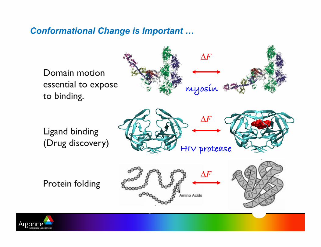
Conformational Change is Important …

Ligand binding (Drug discovery)

HIV protease!

ΔF

Protein folding ΔF

Domain motion essential to expose to binding.

myosin!

ΔF

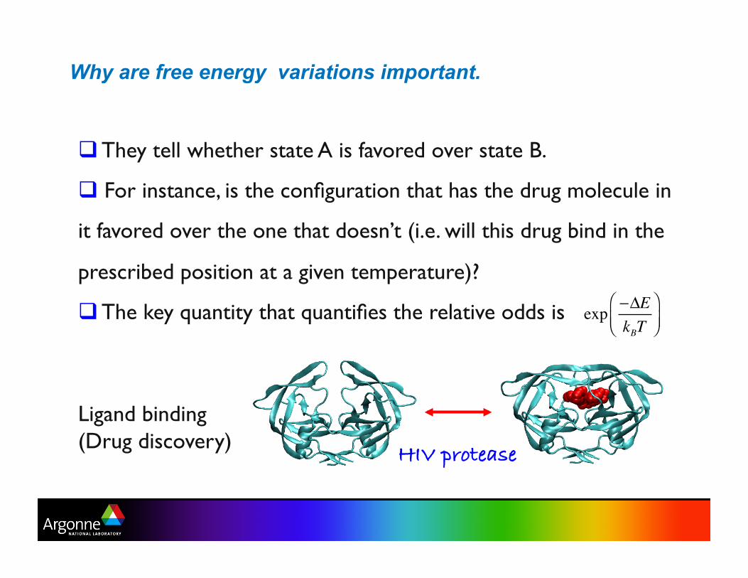
Why are free energy variations important.

  They tell whether state A is favored over state B.

  For instance, is the configuration that has the drug molecule in

it favored over the one that doesn’t (i.e. will this drug bind in the

prescribed position at a given temperature)?

  The key quantity that quantifies the relative odds is

Ligand binding (Drug discovery)

HIV protease!

exp −ΔEkBT

⎛⎝⎜

⎞⎠⎟

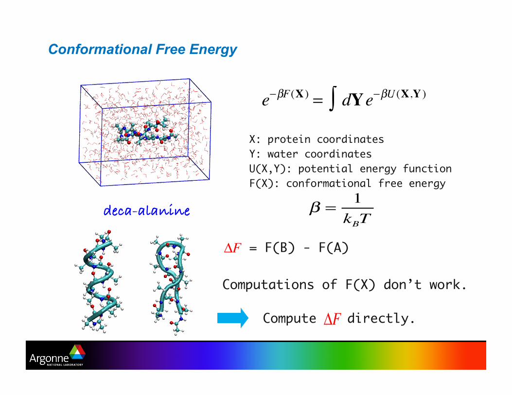
Conformational Free Energy

�

e−βF(X ) = dYe−βU (X,Y )∫X: protein coordinatesY: water coordinatesU(X,Y): potential energy functionF(X): conformational free energy

deca-alanine!

= F(B) - F(A)

Computations of F(X) don’t work.

Compute directly.

ΔF

ΔF

β =1kBT

Why direct computations of the free energy do not work

  Calculations of the free energy are enormously expensive.   We have to average out the water coordinates.   In a box, there are a few thousand water molecules, that is a few thousand water coordinates – and that is for a small protein !!!   One must estimate nasty quadrature over a 1000 dimensional space (for fixed X, the energy function has lots of minima).  This difficulty is known as the curse of dimensionality: The fact that in excessively large dimensions the sample density decreases exponentially.  This is thus, a very hard problem

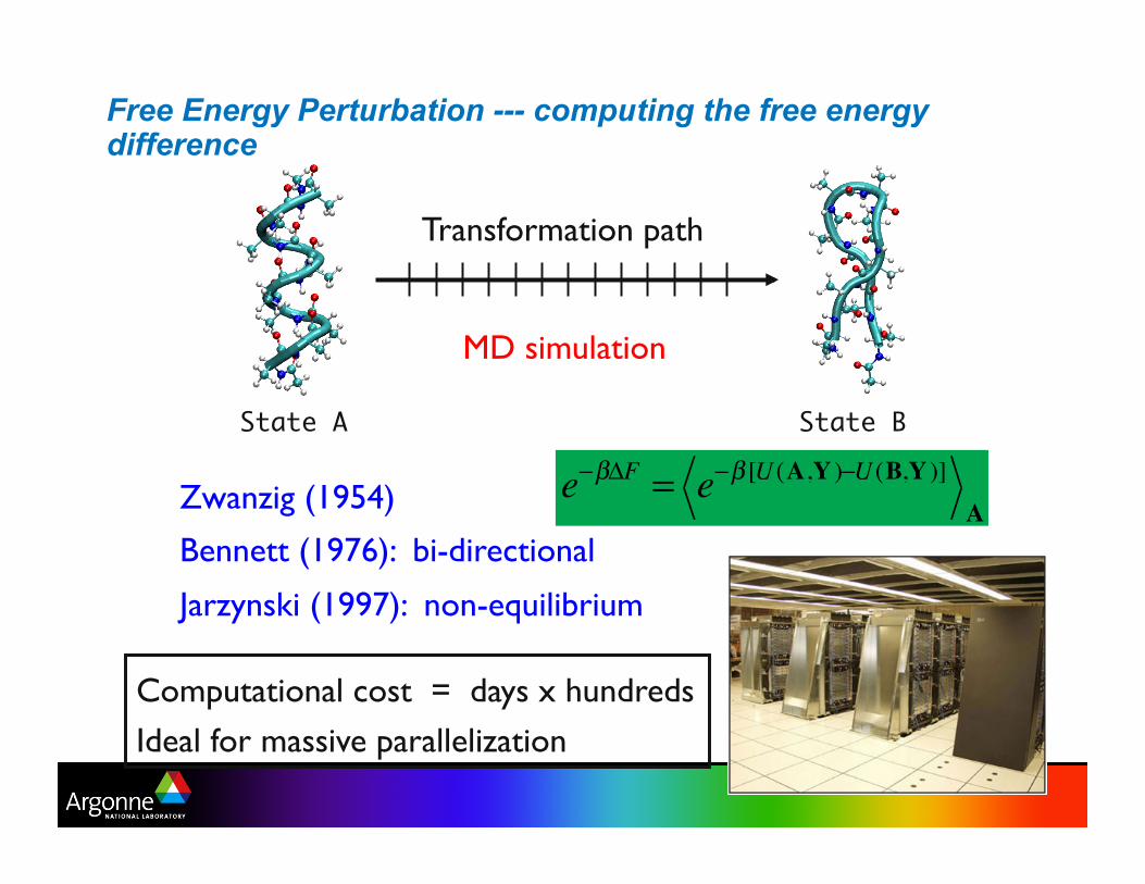
Free Energy Perturbation --- computing the free energy difference

State A State B

Zwanzig (1954)

Bennett (1976): bi-directional

Jarzynski (1997): non-equilibrium

Transformation path

�

e−βΔF = e−β [U (A,Y )−U (B,Y )]A

MD simulation

Computational cost = days x hundreds

Ideal for massive parallelization

Computing free energy variations

 I have just said that computing free energies is hard, so how is this possible?  The trick is to find a “good” path in the phase space.

  Then divide the path in small segments

  If the path is good, the free energy difference including its variance can be computed relatively easily by using some version of importance sampling   So we have transformed the problem into the one of finding a good path in phase space.

One such path: Direct Morphing

�

xn = (1− λ)an + λ bn0 ≤ λ ≤1

3.6 ± 0.69

Carnot cycle A

B

Thermodynamic Cycle

depends only on the end states, not on the path.

Computer simulations are not bound by reality.

ΔF

Computing Free Energy Between 2 States,

  We sample the distribution of states attached to each potential function – “conformation” – by using molecular dynamics.   E.g., we start a molecular dynamics calculation with the potential function for fixed protein atoms, but moving water atoms, until the simulation “relaxes” and the system can be assumed ergodic.   With the samples we create a free energy estimate using Bennett’s acceptance ration method -- BAR

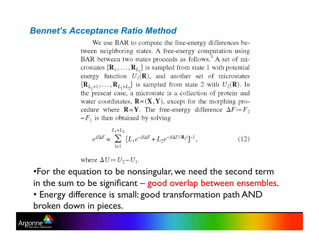
Bennet’s Acceptance Ratio Method

• For the equation to be nonsingular, we need the second term in the sum to be significant – good overlap between ensembles. •  Energy difference is small: good transformation path AND broken down in pieces.

Morphing for Dummies

�

xn = (1− λ)an + λ bσ (n )0 ≤ λ ≤1

Need to find a good path!

Alchemy Alchemy

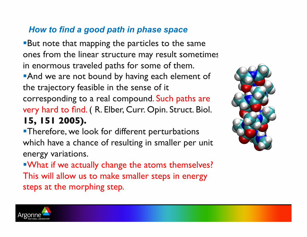
How to find a good path in phase space  But note that mapping the particles to the same ones from the linear structure may result sometimes in enormous traveled paths for some of them.  And we are not bound by having each element of the trajectory feasible in the sense of it corresponding to a real compound. Such paths are very hard to find. ( R. Elber, Curr. Opin. Struct. Biol. 15, 151 2005).  Therefore, we look for different perturbations which have a chance of resulting in smaller per unit energy variations.  What if we actually change the atoms themselves? This will allow us to make smaller steps in energy steps at the morphing step.

Morphing for Dummies

�

xn = (1− λ)an + λ bσ (n )0 ≤ λ ≤1

Minimize the distances !

Alchemy Alchemy

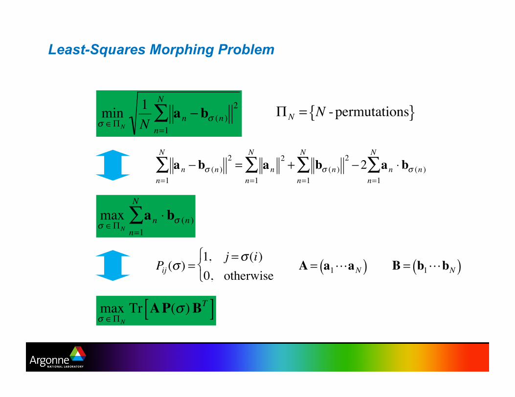
Least-Squares Morphing Problem

�

minσ ∈ΠN

1N

an − bσ (n )2

n=1

N

∑

�

ΠN = N -permutations{ }

�

maxσ ∈ΠN

an ⋅bσ (n )n=1

N

∑�

an − bσ (n )2

n=1

N

∑ = an2

n=1

N

∑ + bσ (n )2

n=1

N

∑ −2 an ⋅bσ (n )n=1

N

∑

�

maxσ ∈ΠN

Tr AP(σ )BT[ ]

�

Pij (σ ) =1, j =σ (i)0, otherwise⎧ ⎨ ⎩

A = a1aN( ) B = b1bN( )

Linear-Programming Solution

�

P1: maxP∈ΩN

Tr APBT[ ]Original problem - Combinatorial search

�

P2 : maxW∈ΓN

Tr AWBT[ ]

�

ΓN = N ×N bistochastic matrices{ }Wij ≥ 0 Wiji∑ =1 Wijj∑ =1

Relaxed problem - Linear programming

�

ΩN = N ×N permutation matrices{ }

Birkoff ’s theorem:

�

ΩN = {Vertices of ΓN }

Fundamental theorem of LP:

�

Solution of P2 ∈ {Vertices of ΓN }

Another way to look at it – it is a linear assignment problem!

max wijj = 1

N∑

i = 1

N∑ ai ,bj

wijj = 1

N∑ = 1, i = 1,2,…,N; wiji = 1

N∑ = 1, j = 1,2,…,N

wij{ }i, j = 1,2…,N ∈FN ,wij ∈{0,1},i, j = 1,2,…,N

max wijj = 1

N∑

i = 1

N∑ ai ,bj

wijj = 1

N∑ = 1, i = 1,2,…,N; wiji = 1

N∑ = 1, j = 1,2,…,N

wij ≥ 0, i, j = 1,2,…,N

Define A = aji{ }i=1, p; j=1,N

B = bji{ }i=1, p; j=1,N

It is a linear assignment problem !

But we had to identify this in the LS formulation!!

Least-Squares Permutation

200 points

Least-Squares Morphing

3.8 ± 0.44

Direct vs. Least-Squares Morphing

3.6 ± 0.69

Direct Least-squares

RMS distance = 8.4 Å RMS distance = 2.1 Å

3.8 ± 0.44

Discussion of the results.

  Each one of the steps in the molecular dynamics simulation is done with NAMD.   NAMD is enormously expensive. One free energy perturbation step (FEP) takes 20 CPU hours for the deca-alanine.   In this case, dummying the atoms takes 10 FEP, our least-squares morphing takes 10 FEPs, and the un-dummying of the atoms takes another 10 FEPs. Compare with 50 FEP steps for the original step. We save 600 CPU hours. (Morphing with LP takes 1-2 seconds).  We solve 2 linear programming – linear assignment problems. There are better ways to do linear assignments, but, give the small computational cost, it is not worth to do it.   But, more importantly, we can compute a more accurate path 0.44 versus 0.69 kcal/mol.

About NAMD– Molecular Dynamics Software

•  Why it is difficult: very expensive potential – CHARM 22.

• Simulations done at constant temperature, using the Langevin thermostat and Langevin-piston barostat. • Time step: 1fs, it is run for 1ns (1000 steps !), the trajectories sampled at 100fs are used as samples for estimating the integral.

Why computing a path of small error is not trivial

  We note that getting a good path is still a matter of heuristics.   We are interested in the overall error, not just the asymptotic

error estimate for one segment, which may have the usual Monte Carlo behavior.

  Therefore it is not clear how the estimate behaves with more segments – therefore the cost of reducing the error for the original approach to the level we have obtained is hard to fathom.

  We have to some extend added a new capability to molecular dynamics.

WW Domain Direct morphing

RMS distance = 11.3 Å100 FEP steps12.9 ± 3.2 kcal/mol

Least-squares morphing

RMS distance = 3.4 Å50 + 30 FEP steps13.3 ± 1.1 kcal/mol

To our knowledge, this is the first time the WW domain protein has been computed at all with this low of an error estimate.

Conclusion

  Morphing can result in much sharper estimates of free energy differences between different conformations.  We have shown that least-square morphing obtains an excellent free energy perturbation path.  We have shown that the path can be obtained in polynomial time, by using linear programming – linear assignment.  We have obtained 100s of CPU hour computational time savings, with much more accurate FE difference estimates.

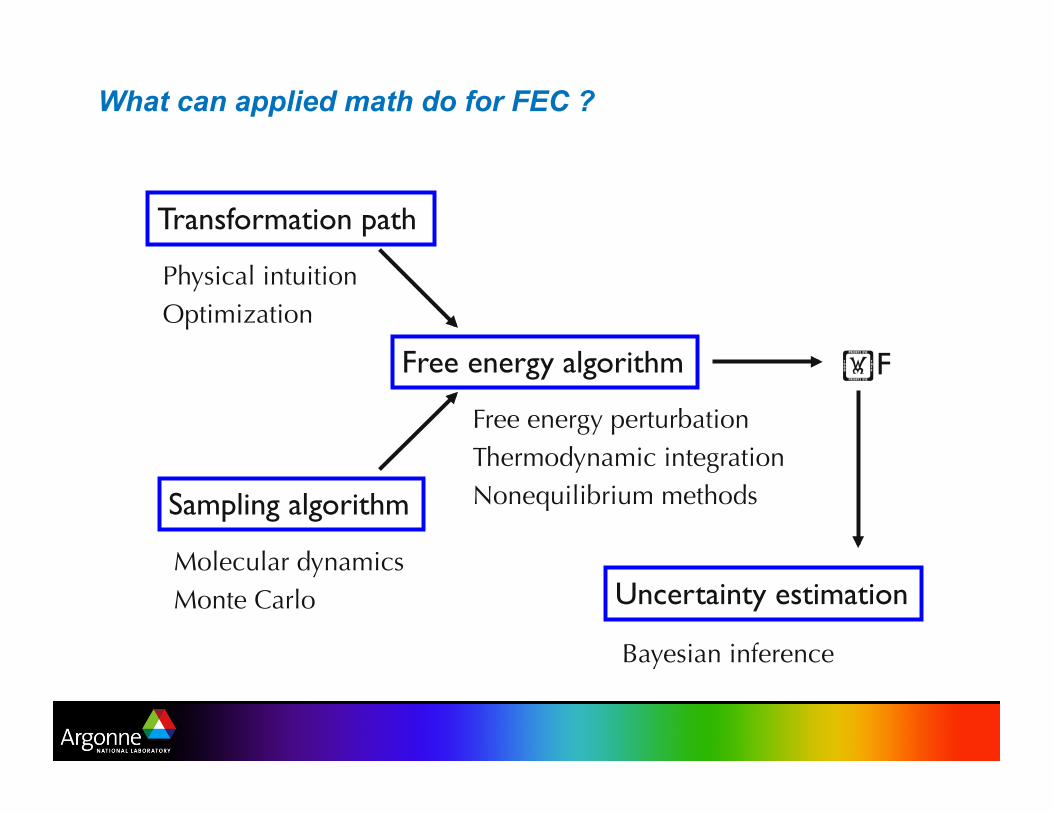
What can applied math do for FEC ?

Transformation path

Sampling algorithm

F Free energy algorithm

Molecular dynamics Monte Carlo

Physical intuition Optimization

Free energy perturbation Thermodynamic integration Nonequilibrium methods

Uncertainty estimation

Bayesian inference