A Linear Programming Approach to Semide nite Programming ...
44
A Linear Programming Approach to Semidefinite Programming Problems John E. Mitchell Department of Mathematical Sciences Rensselaer Polytechnic Institute Troy, NY 12180 USA [email protected] http://www.rpi.edu/˜mitchj Joint work with Kartik Krishnan. IBM Yorktown Heights 6 April 2001
Transcript of A Linear Programming Approach to Semide nite Programming ...

A Linear Programming Approach to
Semidefinite Programming Problems
John E. Mitchell
Department of Mathematical Sciences
Rensselaer Polytechnic Institute
Troy, NY 12180 USA
http://www.rpi.edu/˜mitchj
Joint work with Kartik Krishnan.
IBM Yorktown Heights
6 April 2001

Solving SDP via LP 1
Abstract
A semidefinite programming problem can be regarded
as a convex nonsmooth optimization problem, so it can be
represented as a semi-infinite linear programming prob-
lem. Thus, in principle, it can be solved using a cutting
plane approach; we describe such a method. The cutting
plane method uses an interior point algorithm to solve
the linear programming relaxations approximately, be-
cause this resulted in the generation of better constraints
than a simplex cutting plane method.
Further, the bundle method of Helmberg and Rendl
can be used to generate a set of linear constraints. Typ-
ically, these alone are not sufficient to give a good linear
programming relaxation. Nonetheless, if they are used in
conjunction with some families of problem specific con-
straints, tight LP relaxations can be obtained.

Solving SDP via LP 2
Contents
1. Introduction.
2. A semi-infinite linear program.
3. Dual vs primal.
4. Regaining a primal SDP solution.
5. The bundle method.
6. Computational results using the bundle method.
7. Finding violated constraints.
8. Cutting plane results.
9. Conclusions.

Solving SDP via LP 3
1 Introduction
Standard form:
min C • X
subject to A(X) = b (SDP )
X � 0,
with dual
max bTy
subject to ATy + S = C (SDD)
S � 0
• X and S are square matrices.
• Constraints require that X and S be positive semidef-
inite.
• Inner products are the Frobenius inner product.
• AX =
A1 • X...
Ak • X
, ATy =
∑ki=1 yjAj, where each Aj
is a symmetric matrix.
• C is symmetric and b is an k-vector.
• Primal-dual interior point approaches are
limited in the size of problems they can solve.

Solving SDP via LP 4
2 A semi-infinite linear program
• (SDP ) and (SDD) are convex programming prob-
lems.
• Only nonlinearity is the positive semidefiniteness (PSD)
requirement.
• Replace PSD constraint by linear constraints.
��
��
������
Feasible region

Solving SDP via LP 5
Primal formulation:
min C • X
subject to A(X) = b
dTXd ≥ 0 ∀d with ||d||2 = 1.
• Since X is n × n and symmetric, we have a linear
program in n(n+1)2
variables.
• Need to be selective with the vectors d included in
the constraints. For example, use a cutting plane
approach to select vectors d.
• Typically, we will need some vectors d that are dense,
leading to a dense linear programming problem.

Solving SDP via LP 6
Dual formulation:
max bTy (LDD)
subject to dT (C −ATy)d ≥ 0 ∀d with ||d||2 = 1.
• If (SDP ) has k constraints, then (LDD) has k vari-
ables.
• Need to be selective with the vectors d included in
the constraints. For example, use a cutting plane
approach to select vectors d.
• Typically, we will need some vectors d that are dense,
leading to a dense linear programming problem.
• Have far fewer variables than in the primal formula-
tion, so get smaller linear programs (although they
are still dense).

Solving SDP via LP 7
3 Regaining a primal solution
• Because the linear programs are smaller, it was more
efficient to work with the dual formulation.
• We only use a finite number of vectors d, so we are
solving a relaxation of the dual:
max bTy (LDR)
subject to dTi (C −ATy)di ≥ 0
for vectors di, i = 1, . . . , m.
• The optimal value to (LDR) gives an upper bound
on the optimal value of (SDP ).
Solving SDP via LP 8
• (LDR) is a relaxation of (SDD). The dual linear
program to (LDR) is a constrained version of
(SDP ).
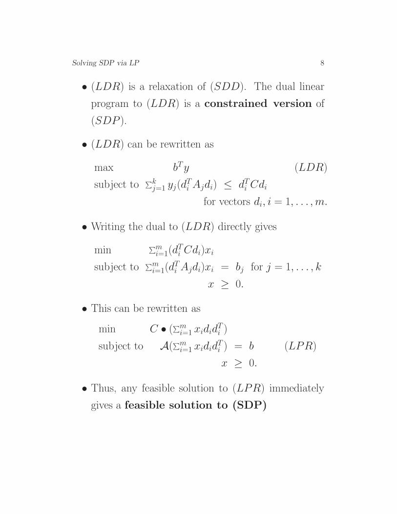
• (LDR) can be rewritten as
max bTy (LDR)
subject to∑k
j=1 yj(dTi Ajdi) ≤ dT
i Cdi
for vectors di, i = 1, . . . , m.
• Writing the dual to (LDR) directly gives
min∑m
i=1(dTi Cdi)xi
subject to∑m
i=1(dTi Ajdi)xi = bj for j = 1, . . . , k
x ≥ 0.
• This can be rewritten as
min C • (∑m
i=1 xididTi )
subject to A(∑m
i=1 xididTi ) = b (LPR)
x ≥ 0.
• Thus, any feasible solution to (LPR) immediately
gives a feasible solution to (SDP)

Solving SDP via LP 9
4 Helmberg’s bundle method
• Need to assume that all feasible solutions X to (SDP )
satisfy trace(X) = a for some (problem dependent)
scalar a.
• Then (SDD) is equivalent to the eigenvalue prob-
lem
maxy aλmin(C −ATy) + bTy
• Solve this problem using a bundle method.
• This requires in the construction of a matrix P (the
current bundle) and the solution of the eigenvalue
problem on a restriction of the feasible region,
maxy aλmin(Pt(C −ATy)P ) + bTy
• This bundle P is refined as the algorithm proceeds.
• At termination, the dual slack matrix C −ATy will
be positive semidefinite on the subspace spanned
by the columns of P , but may well not be positive
semidefinite over the whole of IRn.

Solving SDP via LP 10
One iteration of the bundle method
• Solve the restricted eigenvalue problem using a semidef-
inite programming solver, to obtain y.
• Calculate the function value and a subgradient of the
function for this y.
• The subgradient is found by examining the mini-
mum eigenvalue and corresponding eigen-
vector of C −ATy.
• Update the matrix P .
More about P
• The subgradients are stored as the columns of
P .
• The important subgradients are kept in P , less
important ones are aggregated.
• The number of columns in P is bounded, typi-
cally by the square root of the number of constraints.
Thus, the semidefinite subproblems remain relatively
easy to solve.
• P is orthonormalized at each iteration.

Solving SDP via LP 11
5 Cutting planes from the bundle matrix P
• At termination, the dual slack matrix C −ATy will
be positive semidefinite on the subspace spanned
by the columns of P , but may well not be positive
semidefinite over the whole of IRn.
• The spectral bundle method works well, so it seems
to identify an important subspace on which the
matrix of dual slacks should be psd.
• Directions not in this subspace seem to not be as
important.
• The columns of P are good candidates for the cut-
ting planes di.

Solving SDP via LP 12
Hypothesis 1 In the region of the optimal solution
y∗ to (SDD), the set of vectors y such that the ma-
trix of slack variables is positive semidefinite is closely
approximated by
{y : PT (C −ATy)P � 0}.
Denote the columns of P by pl, l = 1, . . . , r. We have
{y : PT (C −ATy)P � 0}⊆ {y : pT
l (ATy)pl ≤ pTl Cpl, l = 1, . . . , r}.
Empirically, these columns provide a good approxi-
mation to the set of psd slack matrices, if used in con-
junction with additional carefully selected con-
straints.

Solving SDP via LP 13
Rationale
• The optimal matrix of dual slacks, S∗, will have a
nullspace of dimension greater than one.
• This is the eigenspace with smallest eigen-
value.
• If the bundle method is successfully identifying the
optimal matrix of dual slacks, it will also find a basis
for this eigenspace.
• The vectors in this basis will become columns of P .
• For matrices S where the columns of P are eigen-
vectors, stating PTSP � 0 is equivalent to stating
that pTl Spl ≥ 0 for l = 1, . . . , r. (Diagonalization!)
• Matrices close to S∗ will have eigenvectors close to
the eigenvectors of S∗.
• So the weakening of the condition PTSP � 0 may
not be too severe.

Solving SDP via LP 14
6 Maxcut problems
Divide the vertices of a graph into two sets so that the
number of edges with one endpoint in each set is as large
as possible. SDP relaxation:
max L4• X
subject to diag(X) = e
X � 0,
with dual
min eTy
subject to −Diag(y) + S = −L4
S � 0
Here L = Diag(Ae) − A is the Laplacian matrix of the
graph, where A is the weighted adjacency matrix. Note
that trX = n, the number of nodes in the graph.

Solving SDP via LP 15
Linear constraints
Require dTSd = dT (Diag(y) − L4 )d ≥ 0, ∀d. Use the
following d for the max cut problem.
MC1 Set d = ei , ∀i = 1 . . . n, where ei is the ith
standard basis vector for IRn. This generates the
constraint yi ≥ Lii4
, ∀i = 1 . . . n.
MC2 Set d = (ei±ej) , ∀ edges (i, j) gives the constraint
yi + yj ≥ Lii4 +
Ljj
4 + |Lij2 |.
MC3 The columns pi, i = 1, . . . , r of the bundle matrix
P .
We consider two LP relaxations:
• LP1 containing MC1 and MC3.
• LP2 containing MC2 in addition to the constraints
in LP1.
Sol
vin
gSD
Pvia
LP
16
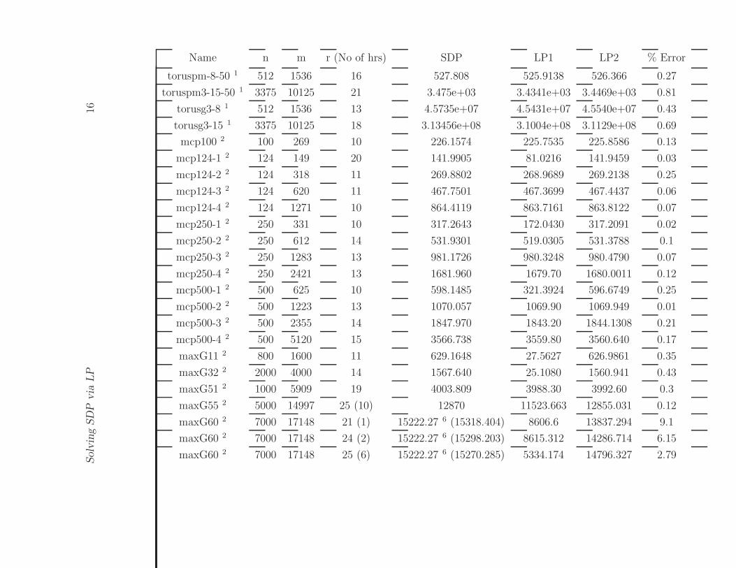
Name n m r (No of hrs) SDP LP1 LP2 % Error
toruspm-8-50 1 512 1536 16 527.808 525.9138 526.366 0.27
toruspm3-15-50 1 3375 10125 21 3.475e+03 3.4341e+03 3.4469e+03 0.81
torusg3-8 1 512 1536 13 4.5735e+07 4.5431e+07 4.5540e+07 0.43
torusg3-15 1 3375 10125 18 3.13456e+08 3.1004e+08 3.1129e+08 0.69
mcp100 2 100 269 10 226.1574 225.7535 225.8586 0.13
mcp124-1 2 124 149 20 141.9905 81.0216 141.9459 0.03
mcp124-2 2 124 318 11 269.8802 268.9689 269.2138 0.25
mcp124-3 2 124 620 11 467.7501 467.3699 467.4437 0.06
mcp124-4 2 124 1271 10 864.4119 863.7161 863.8122 0.07
mcp250-1 2 250 331 10 317.2643 172.0430 317.2091 0.02
mcp250-2 2 250 612 14 531.9301 519.0305 531.3788 0.1
mcp250-3 2 250 1283 13 981.1726 980.3248 980.4790 0.07
mcp250-4 2 250 2421 13 1681.960 1679.70 1680.0011 0.12
mcp500-1 2 500 625 10 598.1485 321.3924 596.6749 0.25
mcp500-2 2 500 1223 13 1070.057 1069.90 1069.949 0.01
mcp500-3 2 500 2355 14 1847.970 1843.20 1844.1308 0.21
mcp500-4 2 500 5120 15 3566.738 3559.80 3560.640 0.17
maxG11 2 800 1600 11 629.1648 27.5627 626.9861 0.35
maxG32 2 2000 4000 14 1567.640 25.1080 1560.941 0.43
maxG51 2 1000 5909 19 4003.809 3988.30 3992.60 0.3
maxG55 2 5000 14997 25 (10) 12870 11523.663 12855.031 0.12
maxG60 2 7000 17148 21 (1) 15222.27 6 (15318.404) 8606.6 13837.294 9.1
maxG60 2 7000 17148 24 (2) 15222.27 6 (15298.203) 8615.312 14286.714 6.15
maxG60 2 7000 17148 25 (6) 15222.27 6 (15270.285) 5334.174 14796.327 2.79

Solving SDP via LP 17
The columns in the tables represent
n: Problem size i.e. the number of nodes in the graph.
k: Number of SDP constraints.
m: Number of edges in the graph.
r: Bundle size, the number of columns in P.
% Error: |SDP−LPSDP
× 100|.SDP LP1 LP2: The objective value of the various re-
laxations.
m1 m2: Number of constraints in LP relaxations.
q: Number of equipartitions required.
1DIMACS2SDPLIB3Rendl4Mitchell5Memory exceeded6Spectral bundle failed to terminate

Solving SDP via LP 18
Notes on maxcut results
• In most cases LP1 alone provides a fairly good ap-
proximation to the SDP objective value.
• For problems mcp124-1, mcp500-1, maxG11, maxG32
we need to work with the relaxation LP2. These ex-
amples underline the importance of the m rank 2
constraints in LP2. The LP relaxation LP2 pro-
vides an excellent approximation to the SDP
with the %error well below 1% of the SDP objec-
tive value.
• The bundle approach fails to converge for problems
maxG55 and maxG60.
• For the maxG55 problem we run the bundle code for
10 hours. The bundle approach attains an objective
value of 12870 (reported SDP objective in SDPLIB
is 9999.210). Moreover since the LP relaxations LP1
and LP2 are larger than 9999.210 it appears that the
reported solution in SDPLIB is incorrect.
• For the maxG60 problem we consider three runs with
the bundle code, of durations 1 hour, 2 hours and 6
hours respectively. It is seen that longer the run,
the closer the bundle objective to the SDP objective
value, and also tighter is the LP2 relaxation.

Solving SDP via LP 19
Name SDP LP1 LP2
k n m1 m2
toruspm-8-50 512 512 528 2064
toruspm3-15-50 3375 3375 3396 13521
torusg3-8 512 512 525 2061
torusg3-15 3375 3375 3393 13518
mcp100 100 100 110 379
mcp124-1 124 124 144 293
mcp124-2 124 124 135 453
mcp124-3 124 124 135 755
mcp124-4 124 124 134 1405
mcp250-1 250 250 260 591
mcp250-2 250 250 264 876
mcp250-3 250 250 263 1546
mcp250-4 250 250 263 2684
mcp500-1 500 500 510 1135
mcp500-2 500 500 513 1736
mcp500-3 500 500 514 2869
mcp500-4 500 500 515 5635
maxG11 800 800 811 2411
maxG32 2000 2000 2014 6014
maxG51 1000 1000 1019 6928
maxG55 5000 5000 5025 20022
maxG60 7000 7000 7025 24172
Table 1: Sizes of the max cut relaxations
Solving SDP via LP 20
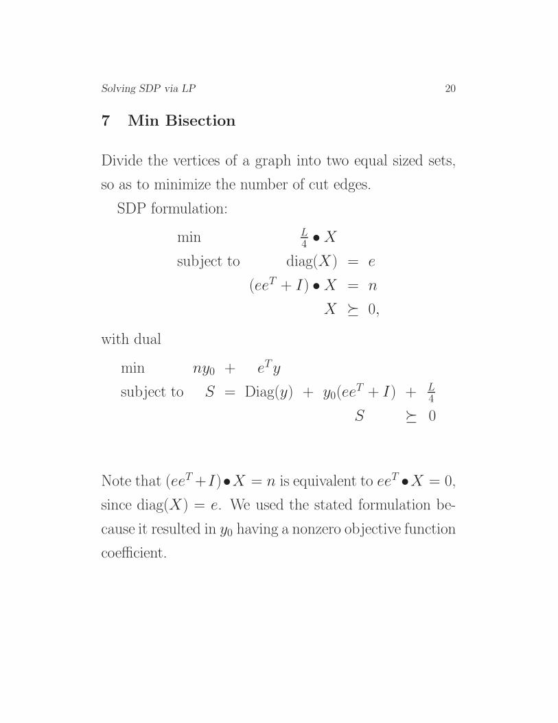
7 Min Bisection
Divide the vertices of a graph into two equal sized sets,
so as to minimize the number of cut edges.
SDP formulation:
min L4• X
subject to diag(X) = e
(eeT + I) • X = n
X � 0,
with dual
min ny0 + eTy
subject to S = Diag(y) + y0(eeT + I) + L
4
S � 0
Note that (eeT +I)•X = n is equivalent to eeT •X = 0,
since diag(X) = e. We used the stated formulation be-
cause it resulted in y0 having a nonzero objective function
coefficient.

Solving SDP via LP 21
Linear constraints:
Need dTSd = dT (y0(eeT + I) + Diag(y) + L
4 )d ≥ 0, ∀d.
MB1 Set d = ei , ∀i = 1 . . . n, gives 2y0 + yi ≥ −Lii4
,
∀i = 1 . . . n.
MB2 Set d = ei−ej , ∀{i, j} ∈ E, gives yi+yj +2y0 ≥Lij2− Lii
4− Ljj
4, ∀{i, j} ∈ E.
MB3 Set d = ei+ej , ∀{i, j} ∈ E, gives 6y0 +yi+yj ≥−Lij
2− Lii
4− Ljj
4, ∀{i, j} ∈ E.
MB4 Set d = e, gives (n2 + n)y0 +∑n
i=1 yi ≥ 0, since
Le = 0.
MB5 The columns pi, i = 1, . . . , r of the bundle ma-
trix P .

Solving SDP via LP 22
Unbounded optimal face
There is a ray in the direction y0 = 1, yi = −1, ∀i =
1, . . . , n. Therefore, we also investigated imposing an
upper bound of u on y0.
Thus, we are in essence solving the following pair of
SDP’s
min
L4 0
0 u
•
X 0
0 xs
subject to diag(X) = e
(eeT + I) • X + xs = n
X 0
0 xs
� 0
with dual
max ny0 + eTy
subject to Diag(y) + y0(eeT + I) + S = L
4
S � 0
y0 ≤ u
Here xs is the primal variable corresponding to the
upper bound constraint y0 ≤ u. Since I • X = n, we
have eeT • X = −xs in the SDP formulation of min
bisection.
Sol
vin
gSD
Pvia
LP
23
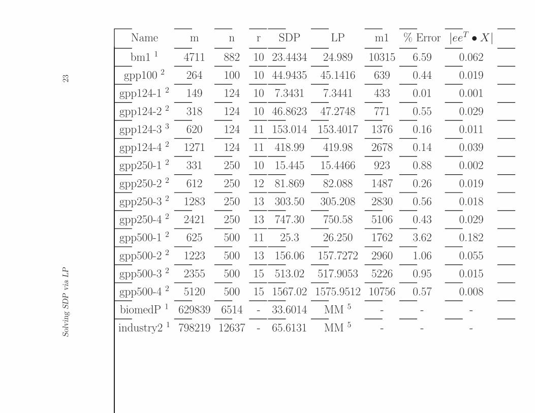
Name m n r SDP LP m1 % Error |eeT • X|bm1 1 4711 882 10 23.4434 24.989 10315 6.59 0.062
gpp100 2 264 100 10 44.9435 45.1416 639 0.44 0.019
gpp124-1 2 149 124 10 7.3431 7.3441 433 0.01 0.001
gpp124-2 2 318 124 10 46.8623 47.2748 771 0.55 0.029
gpp124-3 3 620 124 11 153.014 153.4017 1376 0.16 0.011
gpp124-4 2 1271 124 11 418.99 419.98 2678 0.14 0.039
gpp250-1 2 331 250 10 15.445 15.4466 923 0.88 0.002
gpp250-2 2 612 250 12 81.869 82.088 1487 0.26 0.019
gpp250-3 2 1283 250 13 303.50 305.208 2830 0.56 0.018
gpp250-4 2 2421 250 13 747.30 750.58 5106 0.43 0.029
gpp500-1 2 625 500 11 25.3 26.250 1762 3.62 0.182
gpp500-2 2 1223 500 13 156.06 157.7272 2960 1.06 0.055
gpp500-3 2 2355 500 15 513.02 517.9053 5226 0.95 0.015
gpp500-4 2 5120 500 15 1567.02 1575.9512 10756 0.57 0.008
biomedP 1 629839 6514 - 33.6014 MM 5 - - -
industry2 1 798219 12637 - 65.6131 MM 5 - - -

Solving SDP via LP 24
The value of the dual variable, corresponding to the
upper bound constraint y0 ≤ 1 provides an estimate for
|eet • X|. This value is below 0.1 for all, but one, of the
reported instances.

Solving SDP via LP 25
8 The q-equipartition problem
Divide the n nodes in a graph into q equally sized
sets, so as few edges as possible are cut.
Quadratic program formulation in binary variables:
minV12TraceV TLV
subject to V Te = ge
V e = e
Vij = {0, 1} ∀i, j
• L is the Laplacian matrix of the graph.
• g = nq
• An entry Vij of this matrix is 1 if vertex i belongs to
component j in the partition.

Solving SDP via LP 26
An SDP relaxation is the following
min 12TraceLX
subject to diag(X) = e
Xe = ge
X � 0
This can also be written as
min L2 • X
subject to eieTi • X = 1 ∀i = 1, . . . , n
12(eeT
i + eieT ) • X = g ∀i = 1, . . . , n
X � 0
with dual
min∑n
i=1 yi + g∑n
i=1 yn+i
subject to S =∑n
i=1 eieTi yi +
∑ni=1
12(eeT
i + eieT )yn+i + L
2
S � 0

Solving SDP via LP 27
Linear constraints:
Use the following d:
kEQ1 Set d = ei, ∀i = 1, . . . , n, gives yi + yn+i ≥ −Lii2 ,
∀i.
kEQ2 Set d = e, gives∑n
i=1 yi + n∑n
i=1 yn+i ≥ 0.
kEQ3 Set d = (ei + ej), ∀{i, j} ∈ E, gives yi + yj +
2yn+i + 2yn+j ≥ −Lii2− Ljj
2− Lij.
kEQ4 Set d = (ei − ej), ∀{i, j} ∈ E, gives yi + yj ≥−Lii
2 − Ljj
2 + Lij.
kEQ5 The vectors pi, ∀i = 1, . . . , r in the bundle P .
The constraints in kEQ2 ensure that the yn+i, ∀i =
1, . . . , n don’t take arbitrarily large negative values, mak-
ing the LP unbounded.

Sol
vin
gSD
Pvia
LP
28
Name m n q r (No of Hrs) SDP LP m1 % Error
nfl1 4 496 32 8 9 7.3372e+05 7.3202e+05 1034 0.23
nfl2 4 496 32 4 9 6.2890e+05 6.2890e+05 1034 0
A100 3 4070 100 2 10 8.61803e+05 8.61807e+05 8251 4.6e-04
gpp100 2 364 100 2 10 44.9435 44.9449 839 0.0031
gpp124-1 2 149 124 2 10 7.3431 43.0370 433 486.09
gpp124-1 2 149 124 2 31 7.3431 7.3443 454 0.016
gpp124-2 2 318 124 2 8 46.8623 46.864 769 0.0036
gpp250-1 2 331 250 2 40 (3) 15.445 6 (15.414) 18.757 953
gpp250-2 2 612 250 2 11 81.869 81.872 1486 0.0037

Solving SDP via LP 29
Notes on the q-equipartition results
• The LP relaxation of the bisection problem, i.e. q-
equipartition with q = 2, does not have an unbounded
optimal face, unlike the earlier LP relaxation of min
bisection.
• The bipartition formulation of min bisection gives
an SDP relaxation which is relatively harder to solve
than the original min bisection formulation using the
bundle approach, since we are dealing with more con-
straints.
• Need a larger bundle for gpp124-1, gpp250-1. Can
then get tighter LP approximations to gpp124-1. For
instance, with the default bundle size we are only
able to get an LP approximation of 43.0370 (SDP
objective value is 7.3431), but with the larger bundle
size our LP relaxation is 7.3443 for a %error of 0.016.
However this results in bundle sizes r much larger
than√
k.
Solving SDP via LP 30
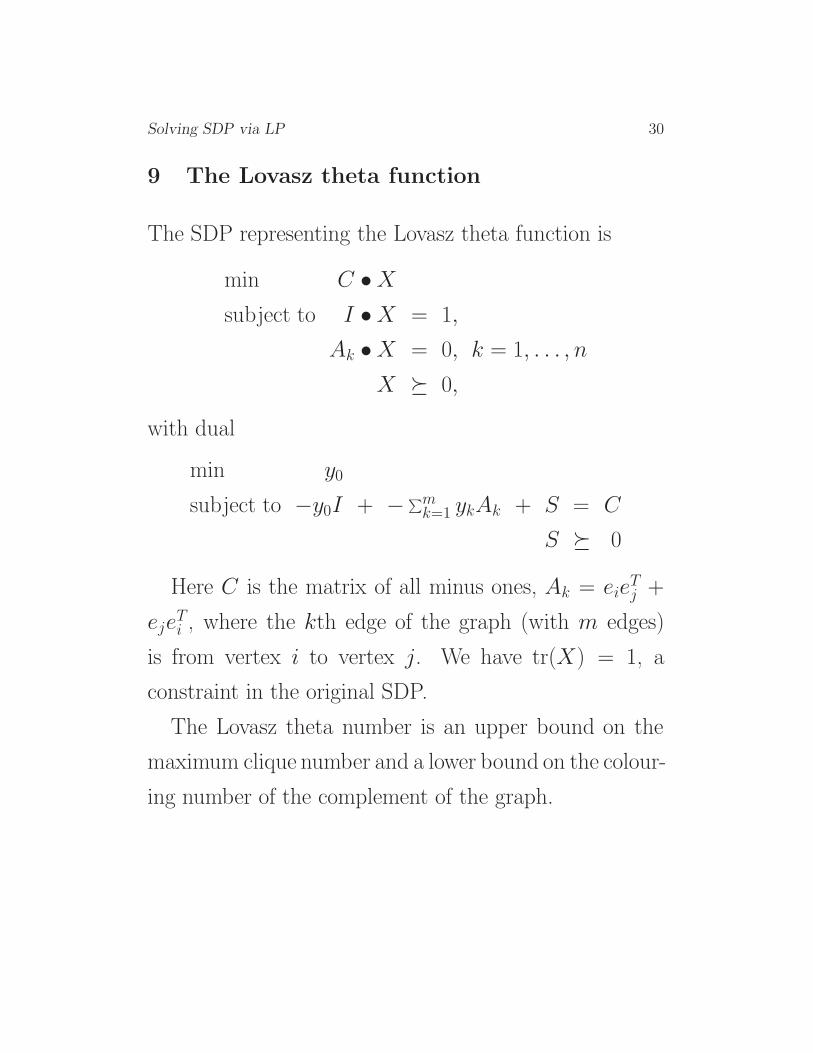
9 The Lovasz theta function
The SDP representing the Lovasz theta function is
min C • X
subject to I • X = 1,
Ak • X = 0, k = 1, . . . , n
X � 0,
with dual
min y0
subject to −y0I + −∑mk=1 ykAk + S = C
S � 0
Here C is the matrix of all minus ones, Ak = eieTj +
ejeTi , where the kth edge of the graph (with m edges)
is from vertex i to vertex j. We have tr(X) = 1, a
constraint in the original SDP.
The Lovasz theta number is an upper bound on the
maximum clique number and a lower bound on the colour-
ing number of the complement of the graph.
Solving SDP via LP 31
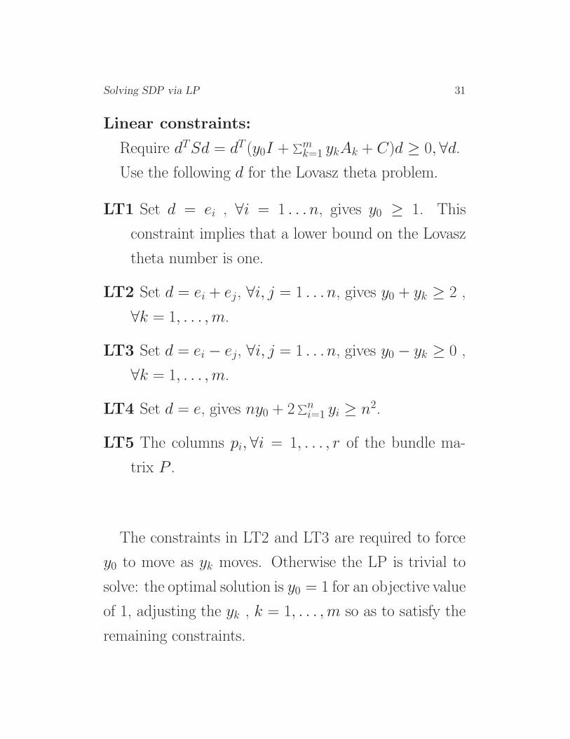
Linear constraints:
Require dTSd = dT (y0I +∑m
k=1 ykAk + C)d ≥ 0, ∀d.
Use the following d for the Lovasz theta problem.
LT1 Set d = ei , ∀i = 1 . . . n, gives y0 ≥ 1. This
constraint implies that a lower bound on the Lovasz
theta number is one.
LT2 Set d = ei + ej, ∀i, j = 1 . . . n, gives y0 + yk ≥ 2 ,
∀k = 1, . . . , m.
LT3 Set d = ei − ej, ∀i, j = 1 . . . n, gives y0 − yk ≥ 0 ,
∀k = 1, . . . , m.
LT4 Set d = e, gives ny0 + 2∑n
i=1 yi ≥ n2.
LT5 The columns pi, ∀i = 1, . . . , r of the bundle ma-
trix P .
The constraints in LT2 and LT3 are required to force
y0 to move as yk moves. Otherwise the LP is trivial to
solve: the optimal solution is y0 = 1 for an objective value
of 1, adjusting the yk , k = 1, . . . , m so as to satisfy the
remaining constraints.

Sol
vin
gSD
Pvia
LP
32
Name m n r (No of Hrs) SDP LP m1 % Error
hamming-9-8 1 2304 512 23 224 221.6829 4633 1.0344
hamming-7-5-6 1 1792 128 12 42.67 42.5297 3598 0.3288
hamming-10-2 1 23040 1024 - 102.4 MM 5 - -
hamming-11-2 1 56320 2048 - 170.67 MM 5 - -
hamming-8-3-4 1 16128 256 43 25.6 25.32 32301 1.0938
hamming-9-5-6 1 53760 512 - 85.33 MM 5 - -
theta1 2 103 50 10 23 22.9503 218 0.2161
theta2 2 497 100 20 32.87 32.8378 1016 0.098
theta3 2 1105 150 25 42.166 40.1389 2237 4.8074
theta3 2 1105 150 47 42.166 42.107 2259 0.14
theta4 2 1948 200 25(6) 50.321 6 (50.35) 38.1189 3923 24.2485
theta4 2 1948 200 51(6) 50.321 6 (50.331) 49.6258 3949 1.3815
theta5 2 3027 250 25(6) 57.232 6 (57.282) 33.3018 6081 41.8126
theta5 2 3027 250 51(6) 57.232 6 (57.576) 51.8651 6107 9.3774
theta5 2 3027 250 51(10) 57.232 6 (57.391) 54.6415 6107 4.7908
theta6 2 4374 300 25(6) 63.477 6 (63.564) 30.061 8775 52.6427
theta6 2 4374 300 59(6) 63.477 6 (65.05) 50.536 8809 20.3869
theta6 2 4374 300 58(10) 63.477 6 (64.316) 54.569 8808 14.0334
theta6 2 4374 300 58(15) 63.477 6 (63.912) 57.27 8808 9.778

Solving SDP via LP 33
Notes on the Lovasz theta experiments
• Since the number of constraints in the Lovasz theta
problem is O(m) a larger bundle is required. Thus
the bundle method is time consuming on these prob-
lems.
• For instance theta3 the bundle approach requires
about 4 hours to converge. It fails to converge for
theta4, theta5, theta6, so we used the bundle from
a 6 hour run. The objective value attained by the
bundle approach is reported in parentheses next to
the SDP objective value.
• To improve on the LP relaxations for the SDPLIB
problems theta3, theta4, theta5 and theta6, we choose
larger bundle sizes, and compute the LP relaxations
using the bundle available after runs of various length.
This considerably strengthens the LP relaxation in
all cases.
• For the DIMACS Hamming instances, the bundle
approach finds the optimal bundle in a few itera-
tions. We are unable to solve to solve hamming-10-
2, hamming-11-2 and hamming9-5-6, where we run
out of memory.

Solving SDP via LP 34
• When the bundle approach converges, our LP solu-
tion is an excellent approximation to the SDP objec-
tive value with the %error well under 1%.
• It must be emphasised here that all the SDPLIB Lo-
vasz theta problems can be solved in under an hour
using any interior point package such as SDPT3.

Solving SDP via LP 35
10 Box constrained QP’s
Consider the the following box constrained QP
max xTQx
subject to −e ≤ x ≤ e
The SDP relaxation of this problem is
max Q • X
subject to diag(X) ≤ e,
X � 0,
with dualmin ety
subject to Diag(y) ≥ Q
y ≥ 0

Solving SDP via LP 36
Linear constraints:
We use the following d.
QPB1 Set d = ei , ∀i = 1, . . . , n gives yi ≥ Qii ∀i =
1, . . . , n. Since Q is typically a p.s.d. matrix, this
can replace the nonnegativity requirement on yi.
QPB2 The columns pi, ∀i = 1, . . . , r in the bundle P .
Name k n r SDP LP m1 % Error
qpG11 2 800 1600 11 1.181e+04 1.1764e+04 811 0.39
gpG51 2 1000 2000 10 2448.659 2434.502 1010 0.57
This LP provides an excellent approximation to the SDP
objective value and has O(n +√
m) constraints.

Solving SDP via LP 37
11 A Cutting Plane Approach
Given a relaxation, it can be tightened by adding more
cutting planes.
1. Solve an LP relaxation of (SDD) to a tolerance τ
on the relative duality gap.
2. Use a Lanczos scheme to approximately find the
(up to) 20 most negative eigenvalues of the matrix S
of dual slacks, and the corresponding eigenvectors dj .
3. If τ is small enough and if the most negative eigen-
value of S is sufficiently close to zero, STOP.
4. Add constraints corresponding to these eigen-
vectors to the LP relaxation, namely dTj (ATy)dj ≤
dTj Cdj .
5. Reduce τ and return to Step 1.
Solving SDP via LP 38
More details of the cutting plane scheme
• Use an interior point code to solve the LP relaxations.
This results in a test point that is more centered,
leading to better constraints and faster convergence
— see the results.
• Choose an initial point that corresponds to a feasi-
ble solution in (SDP ) and (SDD). This leads to a
feasible initial point for the primal and dual linear
programs, and the algorithm then maintains feasibil-
ity.
• This dual feasible point can be found by exploiting
the fact that the trace of X is constant.
• A primal feasible point can often be found by exploit-
ing the structure of the problem.

Solving SDP via LP 39
Starting the cutting plane method from scratch
Parameters:
• Computational results reported for Maxcut.
• Initial relaxation: yi ≥ Lii4
.
• Initial tolerance τ = 1.0.
• Reduce τ by a factor of 0.95 at each outer iteration.
• Run until a specified time (a few hours).
• Run both simplex and interior point cutting plane
schemes. A strictly feasible starting point was chosen
for the interior point solver. LIPSOL used as the
interior point solver and CPLEX6.5 as the simplex
solver.

Solving SDP via LP 40
Name SDP Bundle msb Interior micp Simplex Iter
mcp100 2 226.16 225.85 379 226.06 1052 224.68 200
mcp124-1 2 141.99 141.95 293 140.19 545 100
mcp124-2 2 269.88 269.21 453 265.34 263.76 100
mcp124-3 2 467.75 467.44 755 461.65 809 459.15 100
mcp124-4 2 864.41 863.81 1405 862.17 1438 857.66 200
mcp250-1 2 317.26 317.21 591 310.88 1030 100
mcp250-2 2 531.93 531.38 876 521.572 1204 100
mcp250-3 2 981.17 980.48 1546 966.31 1306 100
mcp250-4 2 1681.96 1680.00 2684 1672.18 1643.11 100
mcp500-1 2 598.15 596.67 1135 546.28 996 40
mcp500-2 2 1070.06 1069.95 1736
mcp500-3 2 1847.97 1844.13 2869
mcp500-4 2 3566.74 3560.64 5635 3499.36 3430.75 60

Solving SDP via LP 41
Notes on the cutting plane results
• The cutting plane method gets bounds comparable
to those found using the bundle LP method, although
it needs more constraints.
• No constraints are dropped.
• The interior point code has a more central iter-
ate, so it is closer to the cone of semidefinite matri-
ces. Therefore, it adds fewer constraints and these
constraints are stronger, than those found using the
simplex approach.
• At the end of the interior point runs, the most neg-
ative eigenvalue is typically on the order of -0.1.
• The iteration counts are upper bounds; the two cut-
ting plane methods may take fewer iterations in the
specified time.

Solving SDP via LP 42
12 Conclusions
• We provide empirical evidence that only a few lin-
ear constraints, polynomial in the problem size n,
are typically required.
• The LP approach is very successful in solving the
max cut and the box constrained QP problems.
• Bounding the min bisection problem works well, with
the value of |eeT • X| very small.
• The {0, 1} formulation of the min bisection problem
which is a q-equipartition problem with q = 2 is not
unbounded. However, the resulting SDP has more
constraints and is more time consuming.
• The spectral bundle approach is time consuming on
Lovasz theta problems. Larger bundle sizes are needed.
Traditional interior point methods usually outper-
form the spectral bundle method.
• In certain instances, we need bundle sizes >√
k to
tighten our LP relaxations.
• The main computational task in the LP approach
is in computing the optimal bundle P . Solving the
resulting LP relaxations is relatively trivial.

Solving SDP via LP 43
References
[1] B. Borchers. SDPLIB 1.2, a library of semidefinite programming test
problems. Optimization Methods and Software, 11:683–690, 1999.
[2] C. Helmberg. Semidefinite programming for combinatorial optimization.
Technical Report ZR-00-34, TU Berlin, Konrad-Zuse-Zentrum, Berlin,
October 2000. Habilitationsschrift.
[3] A. Lisser and F. Rendl. Telecommunication clustering using linear and
semidefinite programming. Technical report, Institut fur Mathematik,
Universitat Klagenfurt, A – 9020 Klagenfurt, Austria, November 2000.
[4] J. E. Mitchell. Realignment in the NFL. Technical report, Mathematical
Sciences, Rensselaer Polytechnic Institute, Troy, NY 12180, November
2000.
[5] G. Pataki and S. H. Schmieta. The DIMACS library
of mixed semidefinite-quadratic-linear programs, 2000.
http://dimacs.rutgers.edu/Challenges/Seventh/Instances/.
[6] K. C. Toh, M. J. Todd, and R. Tutuncu. SDPT3 — a Matlab software
package for semidefinite programming. Optimization Methods and Soft-
ware, 11:545–581, 1999.
[7] Y. Ye. Approximating quadratic programming with bound and quadratic
constraints. Mathematical Programming, 84:219–226, 1999.