A Light Field Camera For Image Based Rendering

by

Jason C. Yang

S.B. Electrical Engineering and Computer Science Massachusetts Institute of Technology, 1999

Submitted to the Department of Electrical Engineering and Computer Science

in Partial Fulfillment of the Requirements for the Degree of

Master of Engineering in Electrical Engineering and Computer Science

at the

Massachusetts Institute of Technology

June 2000

© 2000 Massachusetts Institute of Technology

All rights reserved

Author .................................................................................................................. Department of Electrical Engineering and Computer Science

May 22, 2000

Certified by .......................................................................................................... Leonard McMillan Assistant Professor Thesis Supervisor

Accepted by .........................................................................................................

Arthur C. Smith Chairman, Department Committee on Graduate Theses

2

A Light Field Camera for Image Based Rendering

by

Jason C. Yang

Submitted to the Department of Electrical Engineering and Computer Science

May 22, 2000

in Partial Fulfillment of the Requirements for the Degree of

Master of Engineering in Electrical Engineering and Computer Science

ABSTRACT

The cost of building a digitizing system for image-based rendering can be prohibitive. Furthermore, the physical size, weight, and complexity of these systems has, in effect, limited their use to small objects and indoor scenes. The primary motivations for this project is to reduce the acquisition cost of light-field capture devices and create a portable system suitable for acquiring outdoor scenes. This paper describes the design of such an apparatus using readily available parts. One of the strategies for reducing the system cost has been to rely on software to correct as many of the geometric and photometric inaccuracies as possible. The resulting light field acquisition device can be built for under $200.

The presented light-field acquisition system employs a modified low-cost flatbed scanner. The scanner is interfaced to a standard desktop PC for indoor use or a laptop for outdoor experiments. Focused onto the glass of the scanner is an 8-by-11-grid assembly of one-inch plastic lenses. To make the scanner mobile, the DC power supply is replaced with a 12V lead acid battery. Although the construction of our light-field capture system is simple, the most significant challenges involve the processing of the raw scanner output. Necessary adjustments are color correction and radial distortion removal. Thesis Supervisor: Leonard McMillan Title: Assistant Professor of Electrical Engineering

3

Acknowledgements

First, I would like to thank Professor Leonard McMillan for supporting

this project. His support and guidance over the past few years have been

invaluable.

A big thanks goes out to the rest of the Computer Graphics Group. I

especially want to thank Aaron Isaksen who has given me a lot of helpful

hints and is always willing to lend a hand. I would also like to thank Chris

Buehler for helping out in calibration. The legion of stuffed animals that have

been willing targets for my experiments also deserve acknowledgement.

Further thanks go to Maria, for putting up with me all this time and

especially for the endless pasta, Chinese food, and calzones.

Special thanks go to my parents and brother for their emotional

support and for funding this grand adventure.

4

Table of Contents

1. Introduction....................................................................................................8

1.1 Background ............................................................................................8

1.2 Light Field Rendering..........................................................................10

1.3 Capture Methods..................................................................................11

1.4 Prior Work ...........................................................................................12

1.5 Thesis Contribution..............................................................................14

2. Flatbed Scanner Design ...............................................................................15

2.1 Overview..............................................................................................15

2.2 Scanner Optics .....................................................................................15

2.3 Lighting................................................................................................18

2.4 Mechanics ............................................................................................19

3. Design Overview .........................................................................................21

3.1 The Scanner .........................................................................................21

3.2 Lens Design .........................................................................................22

3.3 Portability.............................................................................................25

3.4 Illumination..........................................................................................25

4. Capture and Image Processing.....................................................................26

4.1 Capturing a Dataset..............................................................................26

4.2 Color Processing ..................................................................................30

4.2.1 Red Hue in Output Images.......................................................30

4.2.1 Color Temperature ...................................................................31

4.2.2 Infrared Light ...........................................................................32

5

4.2.3 Color Correction ......................................................................33

4.2.3.1 Commercial Software Packages ...............................33

4.2.3.2 White Balancing........................................................34

4.2.3.3 Color Correction Profile ...........................................36

4.2.3.4 Color Correction by Adjusting the Curves ...............37

4.3 Radial Distortion..................................................................................41

4.4 Perspective Discrepancies....................................................................42

4.5 Scan Repeatability ...............................................................................44

5. Results..........................................................................................................45

5.1 Scan Time ............................................................................................45

5.2 Color Correction ..................................................................................45

5.3 Images ..................................................................................................48

6. Future Work and Conclusions .....................................................................51

6.1 Future Work .........................................................................................51

6.1.1 Rendering.................................................................................51

6.1.2 CIS Technology .......................................................................51

6.2 Conclusion ...........................................................................................52

A. Matlab Code for White Balancing ..............................................................53

References........................................................................................................54

6

List of Figures 1-1 Geometric modeling and rendering steps .................................................9

1-2 Light Field Rendering.............................................................................10

1-3 Light Field and Lumigraph methods.......................................................13

1-4 Capture device by MIT’s Computer Graphics Group.............................14

2-1 Top down view of the scanning operation..............................................16

2-2 Light path from target to CCD................................................................17

2-3 Illustration of light length to CCD..........................................................17

2-4 Wavelength absorption characteristic of a CCD.....................................18

2-5 Spectral characteristic of fluorescent light..............................................18

3-1 The low cost, light field capture device ..................................................21

3-2 Illustration of focal length and convergence points................................23

4-1 Capture preview in the TWAIN software...............................................26

4-2 8-by-11 raw output sample .....................................................................28

4-3 Sample raw output scan ..........................................................................29

4-4 Spectral characteristics of various light sources .....................................30

4-5 Color temperatures for various light sources ..........................................31

4-6 Wavelength transmittance of the IR filter...............................................33

4-7 Result of using “autolevels”....................................................................34

4-8 Result of white balancing........................................................................35

4-9 ColorChecker calibration chart ...............................................................36

4-10 Red, green, and blue curves for color correction ....................................39

4-11 Results from using the calibration chart and adjusting curves ...............40

4-12 Radial distortion example .......................................................................41

4-13 Radial distortion removal........................................................................42

4-14 Illustration of perspective distortion .......................................................43

5-1 Histograms from the color correction methods ......................................46

5-2 Color correction results...........................................................................48

5-3 8-by-11 scan of MIT’s great dome .........................................................49

5-4 Subset of figure 5-3.................................................................................50

5-5 Subset of a light field taken indoors .......................................................50

7

List of Tables

3-1 Lens Properties ..........................................................................................23

4-1 Sampled subset of the captured color chart ...............................................37

4-2 Raw RGB values for the three calibration points ......................................38

8

Chapter 1

Introduction

1.1 Background

Traditional 3D graphics is based on geometric modeling, where

objects are completely parameterized. For example, Figure 1-1 shows the

process of modeling the streets of Boston and then rendering a nighttime shot.

The first step is to build the geometric model represented in the figure by

wireframes. Geometry could become even more complicated if people and

cars are added. Next, textures are mapped onto the geometry, increasing the

realism of the scene. Finally, light sources are added and their interaction

with the geometric models are calculated to create the final result.

This process brings up two issues of geometric modeling – complexity

and realism. Complexity relates to the geometric parameterization of an

object; to simulate Boson the vertices of all the objects must be determined.

In other words, someone has to model the buildings, cars, people, etc. inside

the computer. Even aided with software tools, this is an extremely time

consuming task and prone to error. Yet, even with an accurate geometric

description the final model lacks realism. To improve the rendered

appearance of models, color and shading are added in addition to texture

mapping where pictures of textures, i.e. skin, bricks, carpet, etc., are mapped

to the geometry. Extremely realistic computer graphics has been

9

(a)

(b)

(c)

Figure 1-1(a) Wireframe model. (b) Texture Mapped. (c) Final rendering.

10

demonstrated in recent movies such as Jurassic Park and Titanic. However, it

may take years of modeling and rendering to achieve this realism.

1.2 Light Field Rendering

The bulk of the time in creating the Boston shot in Figure 1-1 is spent

in modeling the objects and the final process in calculating the lighting

effects. However, looking at just the final result, it would have been easier

and faster to have taken a handheld camera to some rooftop and in seconds

achieve the same shot. Image-based rendering embraces this idea by

eliminating the traditional methods of geometric modeling and exclusively

using images as the underlying representation, hence the term “image-based”

rendering.

Figure 1-2 Light Field Rendering.

11

Light field rendering [12] is one of many methods for image-based

rendering. The basic idea is to generate new images from novel viewpoints

using a two-dimensional array of reference images. Given a plane in space, a

series of images is taken from different viewpoints on this plane. These

images can be treated as an array of rays because for every image, a ray

beginning from the viewpoint on the camera plane can be mapped to each

pixel on the reference image. With a database of rays for various viewpoints

on the plane, new views, not just those restricted to the original plane, can be

generated. The term “light field” comes from this database of rays.

To generate a new viewpoint, a ray is cast in the desired direction from

each pixel of the new viewpoint. In the case of Figure 1-2, the ray of the

desired pixel is behind the original reference plane. For each ray a nearby

image is chosen from which an approximating ray is selected as the pixel to be

used on the new image. These new images can give the feeling of three-

dimensions as different views are extrapolated from the two-dimensional

array of images.

1.3 Capture Methods

There are two ways to create the database of reference images for

image-based rendering – from rendered images or from digitized images. The

first method is to synthetically create the reference images using the

traditional 3D pipeline similar to the one described earlier. Each image would

12

be rendered with the virtual camera positioned at different locations, such as

on a 2D grid.

The second method is to digitize real-world scenes and objects.

Generally, a digital camera is used to capture images at various positions.

Some limitations regarding this method are accurately determining the

position of the camera for each image and overcoming inherent characteristics

of the camera. The work presented in this paper will focus on the digitizing

method.

1.4 Prior Work

Prior work in image-based rendering includes those of Levoy and

Hanrahan [12] and Gortler, et al. [7]. Figure 1-3 is an illustration Levoy and

Hanrahan’s light field system. It consists of a single camera on a robot arm

that translates in a two-dimensional plane as it captures pictures of an object.

It also uses a narrow field of view lens, so it must rotate the camera toward the

object as it reaches the ends of a horizontal path. One drawback to such a

capture system is the expense of the robot arm and the digital camera. In

addition to the infrastructure costs, such a device also suffers in the time

required to build a dataset. Levoy reported an average of four hours to collect

a dataset.

Gortler, et al.’s lumigraph system, Figure 1-3, employs a handheld

digital camera, which the operator uses to capture pictures of an object at

different angles. The drawback to this system is not in the cost, which lies

13

mostly in the digital camera, but in their rebinning process. Since a user does

not collect images along a precisely defined path they use a rebinning

algorithm to fill in missing information by progressively down-sampling the

data (the pull process) and then building higher resolution images from the

lower resolution ones (the push process). This process, however, alters the

original data so if a scene was later rendered from the viewpoint of a known

camera, the resulting pixels would differ from the original image.

Figure 2-3 (Left) Illustration of the Light Field capture device - a camera on a robot arm. (Right) In the lumigraph system the operator uses a handheld camera and takes pictures to fill the hemisphere around a target.

Isaksen, McMillan, and Gortler [9] have also recently built a light field

digitizer. Their device, Figure 1-4, uses an X-Y platform to translate a

camera, similar to that of [12], but it uses a wide-angle lens so as to avoid

rotating the camera. Again, a drawback to this device is the infrastructure

costs - $3000 for the X-Y platform and $1500 for the camera and lens.

14

Figure 1-4 Computer controlled X-Y platform and digital camera.

1.5 Thesis Contribution

As shown in the previous work, the expense of building a digitizing

system can be prohibitive. This reduces the number of groups able to conduct

image-based rendering research. The motivation for this project is primarily

to reduce the infrastructure costs by using a flatbed scanner as the digitizing

device. A further limitation of the light field systems is that the physical size

of their devices constrains their targets to small objects or indoor scenes.

This paper introduces an apparatus designed using an off-the-shelf

color, flatbed scanner retailing for under $100. The design will also factor in

portability options so as to be able to capture outdoor scenes. Also, by using a

flatbed scanner, the time required to capture a dataset will be reduced to the

limitation of the scanner, which is generally between 1 to at most 15 minutes

at full optical resolution depending on the scanner used.

15

Chapter 2

Flatbed Scanner Design

2.1 Overview

This chapter will cover the internal workings of a typical flatbed

scanner. In order to understand the results and image-processing steps taken

later, one must understand how a scanner works.

Typical flatbed scanners, including the one being used in this design,

are CCD scanners. Basically they use a linear CCD (charged-coupled device)

as the digitizing element. When a scanner is in operation, a light source

illuminates the target object, and rays from the object then pass through the

glass and into an opening in the housing that holds the CCD.

2.2 Scanner Optics

A common misconception regarding CCD scanners is that the size of

the linear CCD is the same as the width of the scanner and that it is positioned

directly underneath the housing opening up near the glass. (Figure 2-1)

However, in actuality, the CCD housing consists of a mirroring system

that directs light to the CCD. The size of the actual linear CCD typically

varies between three to five centimeters. In order to focus the entire width of

a piece of paper onto the CCD the optical path must be lengthened within the

confined space of the scanner. A series of mirrors are used for this purpose.

16

Figure 3-1 Top down illustration of a scanner in operation.

Furthermore, positioned in front of the CCD is a series of lenses,

which directs the incoming light to the CCD. Although this mirroring and

lens system is complicated it actually proves beneficial in scanning objects

with depth, such as when scanning pages in a book where the fold into the

binding and does not reach the glass.

Figure 2-2 is an example of the path of light used by a scanner to reach

the CCD. Every scanner model has a different design, but the basic idea of

folding light with mirrors is the same. Figure 2-3 illustrates the length of the

light path the scanner is trying to fold inside the housing and thus reduces the

size of the scanner. In a typical scanner, the width of an image is about 8.5

inches wide. This is projected onto the smaller area of the CCD. The lens

used for this purpose can have a focal length as far as 450 mm and therefore

17

the CCD housing can contain between three to five mirrors to make the

optical path long enough to correctly focus an image. [13]

Figure 2-2 Ray path from the scanning target (i.e. a photograph) to the CCD.

Figure 2-3 Top down view of the CCD housing. This illustrates the length need to focus

the full width of a scan to the smaller width of the CCD.

18

2.3 Lighting

Scanners operate under fluorescent lighting conditions through a cold

cathode tube. There are several reasons for this design decision. First of all,

cold cathode, fluorescent bulbs last a long time and are power efficient.

Figure 2-4 Wavelength absorption characteristic of a CCD.

Figure 2-5 Spectral characteristic of fluorescent light.

Another reason is due to the spectral characteristics of the CCD

(Figure 2-4) and of fluorescent light (Figure 2-5). CCDs are sensitive to

higher wavelengths of light – red and infrared regions. Therefore, scanners

19

use fluorescent bulbs because they are deficient in that part of the spectrum.

This prevents the capture of information in that region.

However, since the spectral distribution of light is now weighted more

in green and blue than in red, a raw scan would result in an image that is

deficient in red. To compensate for this, scanners adjust the gains for each

RGB color channel.

Scanners have a calibration procedure that they go through either when

they are turned on or before each scan. Exact procedures differ among

manufacturers. In the scanner used in this design there is a black and white

strip of paper used for calibration. (Figure 2-2) Generally, scanners will

calibrate for intensity, meaning it will adjust for the intensity of the

fluorescent light, because the luminous of the bulb is neither constant over

time nor uniform across the bulb.

Scanners also calibrate for color, which is when they adjust for

intensity in each color channel. This is done through white balancing using

the white strip of paper. A description of white balancing will be given in

Chapter Four.

2.4 Mechanics

A belt and a variable speed motor drives the CCD housing of a

scanner. This allows for high speed low resolution scans and slow high

resolution scans.

20

At high resolution, the CCD housing will occasionally stop and back

up. This happens when the output buffer of the scanner is full. At this point

the scanner will stop and wait for the buffer to empty while at the same time

the CCD housing backs up a few steps. This gives the housing time to

accelerate back to normal speed for a consistent scan rate when the scanning

process recommences. [15]

21

Chapter 3

Design Overview

This chapter will describe how to adapt a flatbed scanner for light field

acquisition. The design of a light field, scanning device is shown in

Figure 3-1.

Figure 3-1 Low cost light field capture device.

3.1 The Scanner

The particular flatbed scanner used in this design is the UMAX Astra

2000P (street price is about $70). It is a parallel port scanner with a 600x1200

22

dpi optical resolution at 36 bits of color depth. This means that the CCD has a

maximum density of 600 dpi (along the horizontal scan line) and that scans

occur at minimum increments of 1/1200th of an inch along the scan path. This

scanner was chosen mainly for its high resolution and low cost. We use a

parallel port scanner over faster USB versions for its compatibility with

Windows 95 and NT4.

The scanner’s fluorescent bulb must be disabled so as not to interfere

with environment lighting.

3.2 Lens Design

Mounted above the glass of the scanner is a two-dimensional assembly

of 88 lenses in an 8-row-by-11-column grid. The lenses used are circular

diverging (double-convex) lenses that come on “bug boxes” ($0.50 boxes

used to store and display insects) manufactured by Jp Manufacturing. Table

3-1 gives the specific characteristics of the lens.

The lens grid was constructed by cementing the lenses to each other to

form a flat, two-dimensional array. It would have been ideal to have an entire

sheet of connected lenses manufactured. However, the cost in creating the

mold for such a sheet outstripped the cost of other camera designs. Any

imperfections in the construction of the lens array will be compensated during

the calibration of the camera lenses.

23

PROPERTY MEASUREMENT

Material Acrylic

Index of Refraction 1.49

Radius of Curvature 1.739 in. (44.17 mm)

Lens Diameter 1 in. (25.4 mm)

Thickness (middle) 0.125 in. (3.175 mm)

Back Focal Length 1.6875 in. (42.86 mm)

Field of View 33 degrees

Table 3-1 Lens properties.

The lens array was mounted onto a stiff cardboard box, which is also

mounted to the scanner glass. The lenses are situated such that they are one

focal length away from the glass. This way, images formed by the lenses will

be focused directly onto the glass and will be accurately scanned since the

CCD and internal lenses are focused to the glass.

Figure 3-2 Illustration of various convergence points at a distance of one focal length away from the lens.

Figure 3-2 illustrates this lens arrangement. The focal length is the

distance from the lens where parallel rays entering the lens converge. If a lens

24

is placed at one focal length away from the scanner glass, then every point on

the scanner’s imaging surface will have an associated ray that passes through

the principal point or center of a lens. Therefore, during scanning, there will

exist a ray that passes through the principal point and a point on the glass so

that it reaches the CCD. The created effect is a virtual pinhole camera.

Based on the optical resolution of the scanner and the characteristics of

the lens, the resultant image resolution is about 600x600 pixels for each lens.

The actual usable image, due to the lens’s circular nature, is about 590 pixels

in diameter.

In designing and choosing the lenses, a variety of off-the-shelf

solutions were investigated and compared. The bug lenses were chosen

mainly for their low cost, square form factor, and image quality. Other

solutions included a sheet of Fresnel lenses, which are cheap, plastic,

lenticular lenses used for simple magnification. They are ideal in that they are

manufactured in a grid of multiple lenses. However, the image quality is poor

due to the presence of the lens lines in the scanned images.

More expensive, commercial lenses were tested and compared to the

bug lenses. They produced comparable image quality, but in addition to cost

they also suffered in form factor because they come pre-packaged in their own

housing. Finally, other plastic lenses similar to the bug boxes were tested, but

none had the field of view and ease of use as the bug boxes.

25

3.3 Portability

In order to make the scanner mobile, a 12-Volt lead acid battery is

used as a portable power supply. A laptop is also used to interface with the

scanner. So far, in real-world trials the lead acid battery has been able to

power the scanner through over 30 scans. Based on experience, a single

charge can be expected to last through at least 100 scans, which includes

normal idle power usage and scan previews.

3.4 Illumination

Experiments indicate that the scanner needs a significant amount of

light for capture. Part of the reason for this is that the scanner again assumes

that there is a fluorescent bulb illuminating an object. Since the bulb is in

close proximity to the glass there is significant illumination at the scan.

To adequately illuminate indoor scenes and objects, one or more 500-

Watt halogen bulbs have been used. An advantage of a portable system is the

ability to capture outdoor scenes. Sunlight is extremely capable of

illuminating objects. However, as described in the last chapter, the scanner

calibrates itself based on the brightness of the fluorescent light. In addition to

the imperfections of the bulb, scanners calibrate for brightness to protect the

CCD from over exposure or saturation. Therefore, it is important to take this

into account when targeting outdoors or illuminating indoors, similar to

properly positioning any camera in a lighting environment.

26

Chapter 4

Capture and Image Processing

4.1 Capturing a Dataset

The first few steps in acquiring a light field are the same as in normal

flatbed scanning. The scanner is positioned to target the desired object or

scene. A preview is generally useful to certify that the desired shot is within

the field of view of the lenses. Then, using the TWAIN software that is

packaged with the scanner, a scan is taken. (Figure 4-1)

Figure 4-1 Preview of a light field using the TWAIN software driver for the UMAX 2000P.

27

Initially, scans were taken at the highest optical resolution and color

depth possible, which in this case is 1200x600 dpi at 36 bits of color.

However, referring back to Chapter Two regarding motor speeds and buffer

size, scanning at the highest resolution of the scanner will cause the scanner to

stop intermittently and restart during the scan. This is due to the bandwidth of

the parallel connection and the size of the buffer on-board the scanner. When

the buffer is full, the scanner stops the scan and waits until the buffer is

flushed before it starts again. Although in ideal scanning conditions, such as

when scanning a picture, the starting and restarting of the CCD housing

causes no appreciable side effects because the conditions are controlled and

known. However, in using the scanner as a light-field camera there have been

errors caused by this effect. Therefore, instead of scanning at 36 bits of color,

scans are taken at 24 bits.

Although the color range is not as fine as in the 36 bit color range, 24

bit images allow a continuous movement of the CCD housing and therefore a

smooth and clean scan is achieved. In addition, 24 bit scans result in smaller

file sizes and faster processing time in commercial software.

All scans are saved directly to a Tiff file format to preserve raw data

output. Each scan is 5076 by 6996 in pixels at 600 dpi (8.46 by 11.66 inches),

which is larger than what is expected of an 8-by-11 lens array. This is due to

the area selected for each scan. Instead of focusing on just the image

generated by the lenses a scan is taken of the full scan area. This insures a

28

Figure 4-2 8-by-11 raw output of a calibration board and background.

29

(a)

(b)

Figure 4-3 (a) 5-by-6 raw output scan. (b) Enlarged image of the lens at position (3,4).

30

consistent scan size for all scans and aids in image processing when image

dimensions are constant. The size of each scan file is about 101 MB.

Figures 4-2 and 4-3 are sample raw outputs from the scanner. Clearly

there are problems in the raw output. The following sections will discuss each

image manipulation step and the problem being corrected.

4.2 Color Processing

4.2.1 Red Hue in Output Images

The most glaring problem of the raw output image is the high amount

of red. The cause relates back to the earlier discussion regarding the spectral

sensitivity of CCDs and the spectral distribution of fluorescent light.

Figure 4-4 Spectral characteristics of various light sources: (1) Fluorescent (2) Sunlight (3) Halide Metal Oxide ( 4) Tungsten.

Figure 4-4 gives the spectral power distribution for various light

sources. It has already been noted that fluorescent light does not contain a lot

of red, therefore the scanner compensates by adjusting the gains for the RGB

31

channels. However, when we disable the bulb and operate the scanner in

another lighting environment the scanner will incorrectly adjust the image

colors. For example, the spectral distribution for daylight is relatively even

across the color spectrum, but because the scanner compensates for lack of red

in fluorescent light, the resultant image will contain too much red.

4.2.2 Color Temperature

In addition to spectral characteristics of light there are also color

temperatures to contend with. Temperature, measured in degrees Kelvin,

describes the relation between the degree of heat applied on a light source to

the specified color of light generated. (Figure 4-5)

Figure 4-5 Color temperatures for various light sources.

32

Color temperature can affect the scanner because the scanner is

calibrated for fluorescent light. Different lighting conditions will produce

adverse lighting effects in the output. For example a camera calibrated for

5600 degrees Kelvin (near fluorescent) reproduces light from a 2900 degree

light source (tungsten) with a reddish tint. [3]

4.2.3 Infrared Light

It is also important to consider the spectral sensitivity of CCDs to

infrared (IR) light or wavelengths beyond red light. By using a fluorescent

bulb flatbed scanners are able to compensate for this situation. However,

normal lighting conditions contain a significant amount of infrared light,

especially in tungsten light [5]. Unfortunately, CCDs will capture these

wavelengths. Therefore, in color correction, colors must be adjusted to their

proper levels and extraneous infrared information must be removed.

To remove infrared information an IR cutoff filter is mounted inside

the CCD housing of the scanner before the lens. IR filtering is not just an

issue in this design, but also a universal CCD problem. Digital cameras

usually come standard with hot mirrors (reflects infrared light) or require the

user to install one [5]. Although the amount of transmitted light in the color

spectrum is slightly reduced, the remaining intensities are still sufficient

(Figure 4-6).

33

Figure 4-6 Wavelength transmittance of the IR filter.

4.2.3 Color Correction

4.2.3.1 Correction Through Commercial Software Packages

There are several methods that can be employed to correct the colors

in the output images. One method is to perform automatic correction using an

image-editing software package such as Adobe Photoshop. Figure 4-7 is a

color corrected image after using the “autolevels” feature in Photoshop.

The autolevels feature works by automatically adjusting the highlights,

midtones and shadows, which relates to the bright and dark areas of an image.

Photoshop identifies the lightest and darkest pixels in each color channel and

then proportionally redistributes intermediate pixel values (Photoshop ignores

the first 0.5 % of pixels at the brightest and darkest extremes).

34

Figure 4-7 Image from figure 4-3 after using Photoshop’s “autolevels” tool.

4.2.3.2 White Balancing

The second method of color correction is to white balance the image

using Matlab and its Image Processing Toolbox. This is a similar process

used by the scanner in calibrating for color as discussed earlier.

Like the scanner, the first step is to isolate a white image in the desired

lighting environment. This could be done either by locating areas of white in

our datasets or another option would be to scan a white board or piece of

paper by itself to be used as a reference image.

The next step is to calculate the average value for each color channel,

which is then used to determine a gain factor for the green and blue channels.

green

redgreen µ

µγ =

35

blue

redblue µ

µγ =

The gain factor is then multiplied with every green or blue value. This

basically shifts the blue and green histogram channels so that the peaks line up

with the red channel, which has the higher amount. Figure 4-8 is the resultant

image using our previous example.

Figure 4-8 Color correction using white balancing.

The main obstacle regarding this method is the need for a white

reference scan in every lighting condition the scanner is exposed to. Also,

another problem with this method is that white balancing generally will

correct only for color discrepancies, it will not significantly aid in adjusting

the brightness of the image, which the auto-correction feature in Photoshop

does. It is possible to correct the brightness through a process similar to that

used by the scanner – using black and white patterns. The user can identify

36

areas of white and areas of black and then scale the range between those two

points.

Even though the white-balancing method is accurate and corrects the

color problem, it is generally not a feasible solution because it involves quite a

bit of human input when a more automatic method is desired.

4.2.3.3 Color Correction Profile

Figure 4-9 ColorChecker calibration chart.

The final color correction method is to create a characteristic profile

using a color calibration board. The specific board we use in this design is the

ColorChecker by GretagMacbeth. (Figure 4-9) It is a checkerboard array of

24 scientifically prepared squares of “correct” colors. These boards are used

to compare the color results from photography or electronic publishing. For

example, to calibrate a scanner, a scan of the ColorChecker is taken and then

using Photoshop the captured RGB values are compared to the actual RGB

37

values of the board. A characterization profile can be created from the

differences in the readings, which could then be applied every time the

scanner is used.

Color calibrating the scanner camera proceeds in the same manner.

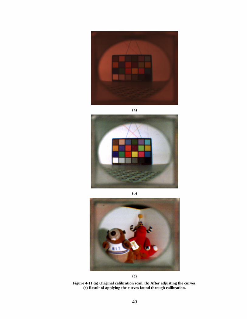
First, a scan is taken of the ColorChecker (see Figure 4-11 for a sample) and

various differences are calculated (Table 4-1). From these measurements a

general profile can be created for the scanner. One method is to use just the

red, green, and blue colors as calibration points. From the calibration data,

those colors are known to be (203,0,0), (64,173,38), and (0,0,142)

respectively. Resultant images are then adjusted so that the red, green, and

blue squares on the scanned pattern match those known values.

Color (chart position) Correct RGB Values Measured RGB Values Blue (Row 3, Col 1) 0, 0, 142 37, 19, 22 Green (3,2) 64, 173, 38 43, 33, 20 Red (3,3) 203, 0, 0 107, 20, 13 Yellow (3,4) 255, 217, 0 115, 45, 18 Magenta (3,5) 207, 3, 124 105, 23, 21 Cyan (3,6) 0, 148, 189 33, 24, 23 White (4,1) 255, 255, 255 140, 60, 41 Middle Gray (4,3) 117, 117, 117 75, 34, 25 Black (4,6) 0, 0, 0 25, 17, 13

Table 4-1 Sampled subset of the captured color chart

4.2.3.4 Color Correction by Adjusting the Curves

Another use of the ColorChecker is to manually adjust the curves

(highlight, midtones, and shadows) of the scanned pattern and then saving

those curves so as to apply them later on new scans. The curves tool is a

standard tool in image-editing software and generally comes in scanning

38

software too. It is a graph of the transfer function or response curve mapping

inputs to output. For example, a curve that is a 45° line is a one-to-one

mapping of inputs to outputs. This method of adjusting the curves is similar

to the way Photoshop processes images using the autolevels command.

The basic idea of the curves method is to use the last row of the

ColorChecker to adjust the white, middle gray, and black colors. A curve is

created that corrects the image so that white has a RGB value of (255, 255,

255), middle gray has a value of (117, 117, 117), and black is mapped to a

RGB value of (0, 0, 0). Table 4-2 gives the raw RGB values of the white,

gray, and black squares measured from a sample image.

White Middle Gray Black

Red 137 72 23

Green 61 34 16

Blue 40 26 13

Table 4-2 Raw RGB values for the three calibration points.

To correct the whites, the pixels in the white square are sampled for

their current values. Then the high end of the curve for each color channel is

adjusted so that each red, green, and blue value of the sampled area is mapped

to 255. Correcting the black values is the same process, the black square is

sampled for initial values and the curve for each color channel is adjusted, but

in this case the low end is changed so that RGB values map to zero.

The final adjustment is a mapping of the gray square. In this step,

initial values for gray are sampled and recorded. Then the middle of the curve

is moved so that in each channel the gray value is mapped to the desired value

39

of 117. For example, the sampled RGB value for middle-gray is (72, 34, 26),

then in the red channel the curve is adjusted so that the middle of the curve

maps the value 72 to 117 and likewise for the green (34 to 117) and blue (26

to 117) channels.

Figure 4-10 Adjusted curves for the red, green, and blue channels.

The final curves (Figure 4-10) are a profile that can be applied to

subsequent images such as in Figure 4-11 for the sample image from before.

However, a potential problem is that since the scanner camera will operate

under different lighting conditions a profile may be needed for each

environment. This is a similar problem to that of the white-balancing method.

40

(a)

(b)

(c)

Figure 4-11 (a) Original calibration scan. (b) After adjusting the curves. (c) Result of applying the curves found through calibration.

41

4.3 Radial Distortion

Figure 4-12 Example of radial distortion in an image. Red lines added afterwards illustrates the severity of curvature radially outward.

Figure 4-11 illustrates the radial distortion caused by the curved nature

of the lenses on the scanner camera. Notice the standard barrel distortion

effect where straight lines bend outward. Radial distortion is a standard

problem in all cameras and can be corrected. The distortion in the scanned

images is more severe than in other cameras because of the inexpensive single

lens optics used for the relatively wide field of view used in the design.

Radial distortion is corrected using methods developed by Lee [11].

The basic idea is to run an optimization procedure on Figure 4-12 to find the

center of mass for each square on the grid and then calculate radial distortion

parameters known as principal points to straighten out the curved lines. From

this, an image can be corrected so that curved lines become straight. (Figure

4-13)

42

Figure 4-13 Image from figure 4-11 after radial distortion correction.

An advantage to this method is that the principal values are constant

for a lens. Therefore, this potentially time-consuming procedure would only

be performed once and the same value can then be applied to subsequent

images.

4.4 Perspective Distortion

Each sub image of the light field camera has a different viewing

frustum. This viewing frustum exhibits a systematic skew along the scan line

direction. Perceptually this skewing appears as a slight rotation. However,

since all sub images share a common image plane this skewing distortion is

better described by a shift of the image center (relative coordinate where the

principal ray crosses the image plane). This skewing of the frustum is

illustrated in Figure 4-14.

43

The explanation for this phenomenon relates back to the optics of the

scanner. In order for the perspective across the scan line to be correct, rays

must enter the CCD housing straight through the glass and straight into the

CCD. However, the rays in the housing are not straight, but are spread wide

due to the internal lens. Rays intersecting the glass towards the extremes will

not correspond to the center axis of the outer lenses and therefore will pick

rays that are rotated outward.

Figure 4-14 Illustration of how light rays reach the CCD. Notice how lenses toward the extremes view outwards instead of straight.

44

This situation is not unlike the light field system [12] where cameras

are pointed inward along a horizontal line. This problem can be corrected

once we calibrate the cameras and determine the intrinsic and extrinsic

properties of the lenses. Once calibrated, the images toward the outer edges

of the scan line can then be mapped to a single plane similar to the light field

system where the rotated cameras have their images mapped to the same

plane.

4.5 Scan Repeatability

In looking at different scans, the position of the images actually

changes from scan to scan, but only in one dimension. This can prove to be

problematic in extracting each image because the method developed in[11]

assumes that images are in a fixed position. Fortunately, even though the

image shifts within a scan, the size of the image does not change. In other

words, the dimensions of the image formed by the lenses remain constant in

different scans. This shifting of the image, which is caused by inconsistencies

in the scanner and scanning software can be corrected by identifying known

points in the image (i.e. corners of lenses) and either shifting the image to a

fixed point or scaling the extraction values in accordance to these reference

points.

45

Chapter 5

Results

5.1 Scan Time

In the prior works discussion, the capture time for light field systems

ranged from 45 minutes to four hours. The scanner camera performs

significantly faster, with a current scan time of 10 minutes (at the highest

possible optical resolution). The scanning time can be reduced further with a

more expensive scanner. Some scanners (between $500 and $1000) are

capable of scanning in under a minute. However, the goal for this project is

low-cost, so the highest quality, inexpensive scanner was used.

The quoted scan time, however, does not include image-processing

time, which adds about half an hour on average to the total scanning time.

Currently image manipulation runs in several stages. It is possible to integrate

all the processing steps so that once a scan is complete, image extraction,

color-correction, and radial distortion removal are performed in one program.

This would reduce a complete scan time from pressing the scan button to a

dataset ready to render to twenty minutes.

5.2 Color Correction

In the last chapter, several color correction methods were outlined and

results were shown. The question is, which method should be employed?

46

(a)

(b)

(c)

(d)

Figure 5-1 Histograms of the (a) original raw output, (b) correction by autolevels, (c) white balancing, (d) and adjustment through curves.

47

Figure 5-1 gives the histograms for the original scan and results of each

correction method. The histogram shows the distribution of values for each

color channel.

White balancing maintains the characteristics of the original

histogram. By finding the averages and scaling each channel using a ratio

with the average red value, the green and blue graphs are just shifted up so

that the peaks line up. When before there was a high amount of red, white

balancing adds more blue and green to compensate.

Using autolevels and correcting through curves basically performs the

same operation since autolevels adjusts the curves automatically. This is why

the histograms for the two are similar. However, the graph characteristics are

different from the original, partly because adjusting the curves produces a

non-linear mapping from inputs to outputs. Therefore, instead of just a shift,

the histograms are scaled and redistributed.

Figure 5-2 shows the results achieved in the last chapter.

Qualitatively, all three methods provide good results. As mentioned before,

the white balancing method does not improve the brightness of the image, but

this can be further corrected in software. Currently, the method being used to

adjust the images is through Photoshop’s autolevels tool, because it is

automatic, fast, and achieves good results (as good as using curves based on

the histograms and the images).

48

(a) (b)

(c) Figure 5-2 (Results from chapter 4 reproduced.)

Correction through (a) autolevels, (b) white balancing, and (c) applying curves.

5.3 Images

Figures 5-3, 5-4, and 5-5 are sample light fields of both an indoor and

an outdoor scene after capture and color correction. We can initially tell that

we have created a light field because we can cross-eye fuse the images into a

three-dimensional view. As seen in figure 5-3, one must be cautious of

saturating the CCD when capturing outdoor light fields. Even so, these final

images show that it is possible to convert a standard flatbed scanner into a

light field capture device.

49

Figure 5-3 8-by-11 scan of MIT’s great dome.

50

Figure 5-4 Subset of figure 5-3.

Figure 5-5 Subset of a light field taken indoors.

51

Chapter 6

Future Work and Conclusions

6.1 Future Work

6.1.1 Rendering

The final goal is to render images taken from the camera introduced in

this paper. There are existing renderers such as those developed by [12] and

[9]. However, those renderers assume that images are evenly spaced in a two-

dimensional plane. Although the images captured by the scanner camera are

on a 2D plane, due to perspective distortion they do correctly map to a dataset

the above renderers can use. Rendering will require calibrating all of the

lenses [11] and using a renderer that does not assume anything about relative

camera positions.

6.1.2 CIS Technology

In designing this camera, one fundamental constraint has been the

linear CCD and the optics that support it. However, new scanners based on

CIS (contact image sensor) technology have emerged in the market. CIS

scanners differ from CCD scanners in that there is no optical system. The CIS

scanning element actually abuts the glass and its length is the full width of the

glass. Therefore, rays come straight into the scanner and go straight into the

CIS and would have no parallax problems.

52

However, CIS scanners do not use fluorescent light as a light source.

Instead they use three rows of red, green, and blue LEDs, which are integrated

with the CIS. Also, before each scan, the scanner runs a complex calibration

procedure between the LEDs and the CIS. Although, CIS scanners would

solve the parallax problem, the hurdle would be to remove the LEDs and

bypass the calibration sequence. In experiments with CIS scanners the LEDs

cannot be removed from the CIS. In order for this technology to work, one

must program a custom TWAIN driver or configure a new scanner from a

separate CIS element.

6.2 Conclusion

This paper has shown that it is possible to develop an inexpensive light

field capture device with a price tag under $200 (not including the laptop). It

has met the primary goal of low cost and is also portable and fast. Although

raw output images have errors, they can be corrected through software. With

the availability of a low-cost light field capture device, image-based rendering

research will hopefully expand into the mainstream.

53

Appendix A

Matlab code for white balancing

Reading in a file:

file = input('Enter file name > ','s');

original = imread(file,'tif');

Calculating scaling factors:

img_mat = input('Enter white image matrix name > ');

dbl_img_mat=im2double(img_mat);

r_ave=mean2(dbl_img_mat(:,:,1))

g_ave=mean2(dbl_img_mat(:,:,2))

b_ave=mean2(dbl_img_mat(:,:,3))

g_gamma=r_ave/g_ave

b_gamma=r_ave/b_ave

Applying the scaling factors:

img_mat = input('Enter image-to-correct matrix name > ');

dbl_img_mat=im2double(img_mat);

dbl_img_mat(:,:,2)=dbl_img_mat(:,:,2)*g_gamma;

dbl_img_mat(:,:,3)=dbl_img_mat(:,:,3)*b_gamma;

fin_img_mat=im2uint16(dbl_img_mat);

Writing out the corrected image:

imwrite(fin_img_mat, ‘corrected_image.tif’,’tif’);

54

References

[1] Devernay and Faugeras, “Automatic Calibration and Removal of Distortion from Scenes of Structured Environments”, SPIE-2567 1995, pp62-72.

[2] “Diagonal 11mm (Type 2/3) Progressive Scan CCD Image Sensor with

Square Pixel for Color Cameras”, Sony Corporation. [3] Dickson, Brad, “Colour Temperature Kelvin Scale”, Society of Television

Lighting Directors, [Online document], 1996, Available HTTP: http://www.stld.org.uk/Colour%20Temperature.htm

[4] Dickson, Brad, “Visible Spectrum Spectral Distribution”, Society of

Television Lighting Directors, [Online document], 1996, Available HTTP: http://www.stld.org.uk/Spectral%20Distribution.htm

[5] “Filters Help Reduce the Red in Digital Pictures Taken in Tungsten

Light”, Kodak Technical Information Bulletin, November 1998. [6] Fulton, Wayne, “Color Correction”, A Few Scanning Tips, [Online

document], 1999, Available HTTP: http://scantips.com/color.html [7] Gortler, S.J., Grzeszczuk, R., Szeliski, R., and Cohen, M., “The

Lumigraph”, Computer Graphics Proceedings, Annual Conference Series (SIGGRPAH 96), pp43-54.

[8] “How to Calibrate Your Scanner”, Mister Print Productions Ltd., [Online

document], Available HTTP: http://www.misterprint.com/scanner.html

[9] Isaksen, A., McMillan, L., and Gortler, L., “Dynamically Reparameterized

Light Fields”, Technical Report MIT-LCS-TR-778, May 1999. [10] “Lamps and Light Sources”, Technical Documentation for UMAX

Service and Repair Centres, Reseller Training and Support Centres, [Online document], Available HTTP: http://support.umax.co.uk/service/lamps.htm

[11] Lee, Charles, “Radial Undistortion and Calibration on an Image Array”,

Master of Engineering Thesis, Massachusetts Institute of Technology, 2000.

[12] Levoy, M., Hanrahan, P., “Light-Field Rendering”, Computer Graphics

Proceedings, Annual Conference Series (SIGGRAPH 96), pp31-42.

55

[13] “Optical Design Considerations”, Technical Documentation for UMAX

Service and Repair Centres, Reseller Training and Support Centres, [Online document], Available HTTP: http://support.umax.co.uk/service/optics.htm

[14] Tsai, R.Y., An Efficient and Accurate Camera Calibration Technique for

3-D Machine Vision, CVPR 1986, pp364-374. [15] Webb, Youngers, Steinle, and Eccher. “Design of a 600-Pixel-per-Inch,

30 Bit Color Scanner”, Hewlett-Packard Journal, February 1997. [16] Zhang, Z.Y., “Flexible Camera Calibration by Viewing a Plane from

Unknown Orientations”, ICCB 1999, pp666-673.