ARTICLE IN PRESS

Journal of Computational Physics xxx (2005) xxx–xxx

www.elsevier.com/locate/jcp

A level-set method for interfacial flows with surfactant

Jian-Jun Xu a,*, Zhilin Li b, John Lowengrub c, Hongkai Zhao c

a Department of Mathematics, Simon Fraser University, Burnaby, BC, Canada V5A 1S6b Center for Scientific Computations and Department of Mathematics, North Carolina State University, Raleigh, NC 27695, USA

c Department of Mathematics, University of California at Irvine, Irvine, CA 92697, USA

Received 31 March 2005; received in revised form 12 July 2005; accepted 15 July 2005

Abstract

A level-set method for the simulation of fluid interfaces with insoluble surfactant is presented in two-dimensions.The method can be straightforwardly extended to three-dimensions and to soluble surfactants. The method couplesa semi-implicit discretization for solving the surfactant transport equation recently developed by Xu and Zhao [J.Xu, H. Zhao. An Eulerian formulation for solving partial differential equations along a moving interface, J. Sci. Com-put. 19 (2003) 573–594] with the immersed interface method originally developed by LeVeque and Li and [R. LeVeque,Z. Li. The immersed interface method for elliptic equations with discontinuous coefficients and singular sources, SIAMJ. Numer. Anal. 31 (1994) 1019–1044] for solving the fluid flow equations and the Laplace–Young boundary conditionsacross the interfaces. Novel techniques are developed to accurately conserve component mass and surfactant mass dur-ing the evolution. Convergence of the method is demonstrated numerically. The method is applied to study the effects ofsurfactant on single drops, drop–drop interactions and interactions among multiple drops in Stokes flow under a steadyapplied shear. Due to Marangoni forces and to non-uniform Capillary forces, the presence of surfactant results in largerdrop deformations and more complex drop–drop interactions compared to the analogous cases for clean drops. Theeffects of surfactant are found to be most significant in flows with multiple drops. To our knowledge, this is the firsttime that the level-set method has been used to simulate fluid interfaces with surfactant.� 2005 Elsevier Inc. All rights reserved.

AMS: 65M06; 65M12; 76T05

Keywords: Incompressible Stokes flow; Interfaces; Insoluble surfactant; Marangoni force; Capillary force; Level set method; Immersedinterface method

0021-9991/$ - see front matter � 2005 Elsevier Inc. All rights reserved.

doi:10.1016/j.jcp.2005.07.016

* Corresponding author.E-mail addresses: jxu@pims.math.ca, jianjunx@cs.sfu.ca (J.-J. Xu), zhilin@math.ncsu.edu (Z. Li), lowengrb@math.uci.edu

(J. Lowengrub), zhao@math.uci.edu (H. Zhao).

2 J.-J. Xu et al. / Journal of Computational Physics xxx (2005) xxx–xxx

ARTICLE IN PRESS

1. Introduction

In this paper, we propose a level-set/immersed interface method for the evolution of deformable fluidinterfaces with insoluble surfactant in two-dimensions. The method can be straightforwardly extended tothree-dimensions and to soluble surfactants. Surfactants are surface-active molecules that selectively adhereto interfaces. Surfactants typically consist of a hydrophilic head and a hydrophobic tail – detergents arecommon examples. Surfactants play a critical role in numerous important industrial and biomedical appli-cations ranging from enhanced oil recovery (e.g. [42]) to pulmonary function (e.g. [16]).

Surfactants are advected and diffused along interfaces by the motion of the fluid and by molecular mech-anisms, respectively [9]. The surface tension depends on the surfactant distribution through the equation ofstate – regions of higher surfactant concentration have lower surface tension. Non-uniform surfactant con-centration along an interface creates non-uniform Capillary (normal) and Marangoni (tangential) forces inthe fluid. This in turn affect the fluid velocity that then couples back to affects the surfactant distribution.For example, the convection of surfactant toward the stagnation points at the tip of a drop tends to lowerthe surface tension there and increase the drop deformation. On the other hand, Marangoni forces resist theconvection of surfactant toward the drop tip and thus restrain the deformation of the drop. Compression/stretching of the interface results in a corresponding increase/decrease in the surfactant concentration.

Computing the motion of interfacial flows with surfactant is challenging. The Navier–Stokes equationsmust be solved in a complex, multiply connected moving domain with prescribed jumps in the normal (Cap-illary) and the tangential (Marangoni) stress across the interface separating the domains. The moving inter-face must be accurately simulated and topology transitions may occur as interfaces reconnect or break-up.Further, as surfactant is advected and diffused along the interface there may be adsorption/desorption ofsurfactant from/to the bulk to/from the interface [9]. For simplicity, we focus here on the case of insolublesurfactant so that the surfactant remains bound to the interface.

In this paper, a level-set method for the simulation of fluid interfaces with insoluble surfactant is pre-sented in two-dimensions. The method couples a semi-implicit discretization for solving the surfactanttransport equation recently developed by Xu and Zhao [62] with the immersed interface method originallydeveloped by LeVeque and Li [31] for solving the fluid flow equations and the Laplace–Young boundaryconditions across the interfaces. Novel techniques are developed to accurately conserve component (do-main) volume and surfactant mass during the evolution. Convergence of the method is demonstratednumerically. The method is applied to study the effects of surfactant on single drops, drop–drop interac-tions and interactions among multiple drops in Stokes flow under a steady applied shear. Due to Marang-oni forces and to non-uniform Capillary forces, the presence of surfactant results in larger dropdeformations and more complex drop–drop interactions compared to the analogous cases for clean drops.The effects of surfactant are found to be most significant in flows with multiple drops. To our knowledge,this is the first time that the level-set method has been used to simulate fluid interfaces with surfactant.

There are now a number of different numerical methods that have been developed to simulate the motionof surface-tension mediated interfacial flows (e.g., see [26]). Popular approaches include boundary integralmethods (e.g., see the reviews [20,48]) where the flow equations are mapped to the interface, front-tracking/continuum surface force (CSF) methods (e.g., see the reviews [15,47,60]) where the flow equations aresolved in the volume domain, a separate mesh is used to describe the interface and nearly singular surfaceforces (continuum surface force) are introduced to approximate the singular surface tension force, volume-of-fluid/CSF methods (e.g., see the review [50]) where a volume-fraction function is used to identify theinterface, level-set/CSF methods (e.g., see the reviews [43,44,51]) where the interface is characterized bythe zero contour of a level-set function and phase-field methods where a concentration field is introducedto identify fluid components (e.g., see the review [3,25,64]). A number of hybrid methods now exist includ-ing level-set/volume-of-fluid methods [56,58], particle level-set methods [12,18], marker/volume-of-fluidmethods [4] and level-contour front tracking methods [52].

J.-J. Xu et al. / Journal of Computational Physics xxx (2005) xxx–xxx 3

ARTICLE IN PRESS

In addition to CSF methods, other flow solvers have been developed that directly account for theLaplace–Young surface tension jump conditions without smoothing. Advantages of such an approach in-clude (1) no introduction of intermediate non-physical states near the interface since the interface conditionis sharp, (2) higher-order accuracy can be achieved as opposed to CSF based methods which are generallyonly first-order accurate. Methods without smoothing include the method developed by Helenbrook et al.[17], the ghost-fluid (GF) method (e.g. [13,38]) and the immersed interface method (IIM, e.g. [19,30,32,35]).These algorithms have the common feature that standard finite difference schemes are used at grid pointsaway from interfaces while the finite difference schemes are modified at grid points near interfaces. In theGF algorithm, subcell resolution is used to mark the interface position and the values of discontinuousquantities are artificially extended to grid points neighboring the interface via extrapolation. A fully sec-ond-order accurate GF method for moving interfaces with geometric boundary conditions has recentlybeen developed [40]. A fourth-order GF method for the Laplace and heat equations has also been devel-oped recently [14]. In the IIM, which is the approach we use here together with a level-set method, a localcoordinate system is introduced to explicitly incorporate jump conditions and discontinuous coefficientsinto second-order accurate finite difference schemes. Advantages of this approach include its high-orderaccuracy, the ease of implementation and the fact that fast solvers (e.g., the FFT) can be used to invertthe discrete systems.

Despite the vast literature on studies of drops and interfaces in multiphase flows, there are relatively fewworks in which the effects of surfactants are incorporated. Much of the previous work on surfactants hasutilized the boundary integral method for axisymmetric (e.g., see [11,41,55]) and 3D (e.g., see [33,48,63])Stokes flows. Recently, CSF-based methods have been developed for interfacial flows with surfactantsusing immersed boundary/front tracking methods [5,22] and volume-of-fluid methods [10,21,49]. We re-mark that in [21], an algorithm was developed to conserve both component mass and surfactant massand is capable of simulating an arbitrary equation of state for the surfactant.

Recently, Xu and Zhao in [62] and Adalsteinsson and Sethian [2] presented methodologies to simulatetransport and diffusion along deformable interfaces in conjunction with a level-set method. In the formerwork, Xu and Zhao applied their algorithm to study specifically the evolution of surfactant although theydid not couple their method to a flow solver. Several test cases were presented in [62] in which a velocity fieldis prescribed. Here, we build upon this work by coupling the transport algorithm of Xu and Zhao to an IIMflow solver. We introduce modifications to conserve component and surfactant mass and we examine the ef-fects of non-uniform Capillary forces and Marangoni forces on the evolution of interfaces in Stokes flow.

The remainder of this paper is organized as follows. The governing equations are presented in Section 2.The numerical method is described in Section 3, which includes the IIM for solving incompressible Stokesflow and the evolution schemes for the surfactant concentration and the level-set function. Numerical sim-ulations are presented in Section 4 to illustrate the performance of the method. Conclusions and futuredirections are discussed in Section 5.

2. The governing equations

2.1. The Navier–Stokes equations

Consider an incompressible two-phase flow consisting of fluids 1 and 2 in a fixed domain X = X1 [ X2

where an interface R separates X1 from X2. In each region, the Navier–Stokes equations govern the fluidmotion

qioui

otþ ðui � rÞui

� �¼ ðr � TiÞT þ qig in Xi ð1Þ

4 J.-J. Xu et al. / Journal of Computational Physics xxx (2005) xxx–xxx

ARTICLE IN PRESS

and

r � ui ¼ 0 in Xi; ð2Þ

where i = 1, 2 denotes the fluid region, Ti ¼ �piI þ liðrui þruTi Þ is the stress tensor, pi is the pressure, qi isthe density, li is the viscosity and g is the gravitational acceleration.

In the far-field, we assume that

u ¼ u1 on oX. ð3Þ

Across the interface R, the velocity is continuous

0 ¼ ½u�R � ujR;2 � ujR;1� �

ð4Þ

and the Laplace–Young jump condition holds [28]

½Tn�R ¼ rjn�rsr; ð5Þ

where r is the surface tension coefficient, n is the normal vector to C directed towards fluid 2, j = $ Æ n is thecurvature of C (positive for spherical/circular interface) and $s = (I � n � n)$ is the surface gradient. Thefirst term on the right-hand side of Eq. (5) is the capillary force and the second is the Marangoni force.

When surfactants are present, the Langmuir equation of state (EOS) [45] is often used to describe therelation between the surfactant concentration f and the surface tension r

rðf Þ ¼ r0 þ RTf1 logð1� f =f1Þ; ð6Þ

where r0 is the surface tension for a clean interface (f = 0), f1 is the surfactant concentration at maximumpacking, R is the ideal gas constant and T is the temperature.

When the actual surfactant concentration f � f1, then the following linear approximation of Eq. (6) canbe used:

rðf Þ ¼ r0 � RTf . ð7Þ

Insoluble surfactants are convected and diffused along the interface. There is no transfer from/to the

bulk either to/from the interface and the total surfactant mass

M ¼ZRf dR ¼

ZXf dR dX; ð8Þ

where dR is the surface delta function, is conserved in time. The local form of the conservation of surfactantmass is [21]

ft þ u � rf � n � ðrunÞf ¼ Dsr2sf ; ð9Þ

where Ds is the surfactant diffusivity. See also [54,61,62] for other forms of Eq. (9).

2.2. The non-dimensionalization and the Stokes system

In this paper, for simplicity, we assume that the two fluids (e.g., drop and matrix) are density- and vis-cosity-matched: q1 = q2 = q and l1 = l2 = l. We also assume that the far-field flow velocity is a simpleshear: u1 ¼ _cyey , where ey is the coordinate vector in the y-direction and _c is the shear rate. To makethe problem dimensionless, we follow [21] and use the characteristic quantities: the radius of a drop a

for length, the inverse shear rate _c�1 for time, the product a _c for velocity, the average surfactant concen-tration fe = 1/|R|�Rf dR for f and the corresponding equilibrium surface tension re = r(fe) for r. By usingthe equilibrium surface tension, rather than the clean surface tension, we scale out the effect of the uniform

J.-J. Xu et al. / Journal of Computational Physics xxx (2005) xxx–xxx 5

ARTICLE IN PRESS

lowering of surface tension that would occur if the surfactant distribution were constant. Thus, by usingthis non-dimensionalization, we emphasize the effect of non-uniform surfactant distribution.

The relevant dimensionless parameters are the Reynolds number Re, the Capillary number Ca, the sur-face Peclet number Pe, the surfactant elasticity E and coverage x

Re ¼ qa2 _cl

; Ca ¼ la _cre

; Pe ¼ a2 _cDs

; E ¼ RTf1r0

; x ¼ fef1

. ð10Þ

For simplicity, in this paper we focus on the case in which the Re = 0 and the inertial terms on the left-handside of Eq. (1) may be dropped. The resulting Stokes system is

Dui ¼ rpi; ð11Þr � ui ¼ 0 ð12Þ

in Xi together with boundary conditions

0 ¼ ½u�R;

� ½p�Rnþ ½ðruþruTÞ � n�R ¼ 1

Caðrjn�rsrÞ

and r is the non-dimensional surface tension given below in Eq. (16). The Stokes equations may be writtenas a system of Poisson equations for the velocity and pressure [32]. The first is the Laplace equation for thepressure which is obtained by taking the divergence of Eq. (11) and deriving the appropriate boundary con-ditions. The result is [32]

r2pi ¼ 0 in Xi ð13Þ

with jump boundary conditions on R

½p�R ¼ � 1

Carj;

opon

� �R

¼ 1

Car2

sr; ð14Þ

and Neumann boundary conditions on oX

opon

¼ r2u � n on oX. ð15Þ

Note that the non-dimensional surface tension r in Eq. (14) is derived from either Eq. (6) or (7) and is given by

rðf Þ ¼ 1þ E lnð1� xf Þ1þ E lnð1� xÞ or rðf Þ ¼ 1� Exf

1� Ex; ð16Þ

respectively.Once the pressure is determined, the velocity is obtained by solving the Poisson system [32]

r2ui ¼ rpi; in Xi ð17Þ

together with the jump boundary conditions

½u�R ¼ 0;ou

on

� �R

¼ 1

Carsr; ð18Þ

and the far-field Dirichlet boundary condition

u ¼ yey on oX. ð19Þ

The Poisson equations for pressure and velocity are exactly in a form appropriate for use with the im-

mersed interface method (IIM). The IIM is described briefly in Section 3.1. The extension of this approachto flows with non-zero Reynolds numbers (but matched viscosities and densities) is straightforward using

6 J.-J. Xu et al. / Journal of Computational Physics xxx (2005) xxx–xxx

ARTICLE IN PRESS

the techniques described in [27,30,37] for the IIM. The extension to flows with variable viscosity has alsobeen recently developed [36].

Finally, the non-dimensional form of the surfactant equation is identical to Eq. (9) with Ds replaced by1/Pe.

2.3. Interface representation

To represent the interface, it is convenient to use the level-set approach. The level-set method was intro-duced by Osher and Sethian [44] and has become an increasingly popular method for simulating multifluidflows (e.g., see the recent reviews [43,51]).

Let /(x, t) be a scalar function whose zero level set {x: /(x, t) = 0} represents the interface R. For exam-ple, we may set /(x, t) to be the signed distance from the point x to R at time t. Since the interface moveswith the fluid, we may take

o/ot

þ u � r/ ¼ 0. ð20Þ

That is, all level surfaces of / move with the fluid. In practice, this causes spatial compression/expansion ofthe level surfaces which is detrimental for accurate interface resolution (e.g. [57,59]). To avoid this, the level-set function is re-initialized after each time step to be a signed distance function locally near the interface[57,59]. This is performed by solving the following Hamilton–Jacobian equation to steady-state

/s þ Sð/0Þðjr/j � 1Þ ¼ 0;

/ðx; 0Þ ¼ /0ðxÞ;

�ð21Þ

where /0 is the level-set function before the re-initialization, and the s is the pseudo-time and S(x) is the signfunction of x defined as

SðxÞ ¼�1 if x < 0;

0 if x ¼ 0;

1 if x > 0.

8><>: ð22Þ

In practice, the re-initialization is performed at every time step.One of advantages of the level-set method is that geometrical quantities can be easily computed. Assume

that the set of x such that /(x, t) < 0 is contained in X1, then the outward normal, curvature and surfacedelta function of the interface R are

n ¼ r/jr/j ; j ¼ r � r/

jr/j

� �; dR ¼ dð/Þjr/j; ð23Þ

where d(x) = dS/dx is the usual one-dimensional delta function.

3. The numerical method

3.1. The immersed interface method

The Stokes equations are solved using the IIM. Let {xi,j = (xi, yj): 0 6 i 6 N, 0 6 j 6 N1} denote a uni-form Cartesian mesh. Let h be the step size in both x- and y-directions. The resulting scheme is an approx-imate projection method in that the velocity field is not exactly divergence-free on the discrete level.

J.-J. Xu et al. / Journal of Computational Physics xxx (2005) xxx–xxx 7

ARTICLE IN PRESS

A grid point xi,j is called irregular if the level-set function / changes the sign from xi,j to its four neigh-bors xi+1,j, xi�1,j, xi,j+1, and xi,j�1, otherwise it is called regular. At an irregular grid point, conventional(central) finite difference scheme may not be accurate since the stencil contains grid points from both sidesof the interface and the solution and/or its derivatives may be discontinuous across the interface.

The idea of the IIM is to design truly second-order accurate finite difference schemes at all points- bothregular and irregular. The schemes explicitly incorporate the jump conditions while maintaining standardforms of the discrete system so that fast solvers can be used. We refer the readers to [19,31,34] for the de-tailed construction of such finite difference schemes at irregular grid points. Here, we highlight the mainidea by illustrating the scheme applied to a Poisson equation

Dw ¼ f

with jump conditions

½w�R and ½ow=on�R given.

Using the IIM, the finite difference scheme, applied to the above equation, is simply the following:

wðxiþ1; yjÞ þ wðxi�1; yjÞ þ wðxi; yjþ1Þ þ wðxi; yj�1Þ � 4wðxi; yjÞh2

¼ f ðxi; yjÞ þ Ci;j þ Ei;j; ð24Þ

where Ei,j is O(h2) at regular grid points, and is O(h) at irregular grid points, the correction term Ci,j is zeroat regular grid points but is non-zero at irregular grid points and depends on the jumps [w]R and [ow/on]R.Note that a fast Poisson solver such as the FFT can be used for solving the discrete system (24). The der-ivation of the correction terms Ci,j involves the following:

� Identify the control points x* = (x*, y*)T associated with each irregular point x = (xi, yj)T. We take

x* = (x*, y*)T to be the orthogonal projection of x = (xi, yj)T on the interface (e.g. [19]).

� Use the Taylor expansions of w(xi, yj), w(xi+1, yj), w(xi�1, yj), w(xi, yj+1), and w(xi, yj�1) at the controlpoints x* up to second-order derivatives from the each side of the interface.

� Use the interface relations to represent all the quantities (up to second-order derivatives) after the Taylorexpansions from one particular side in terms of those from the other.

� Solve for Cij in (24) after the procedures above and ignoring higher-order terms to get the correctionterm.

The interface relations are derived from the two given jump conditions, their surface derivatives, and thedifferential equations. The interface relations and the derivation can be found in [31,34].

Remark. For an elliptic equation with discontinuous coefficients, additional grid points ðxiþi0 ; yjþj0ÞT, with

i0; j0 ¼ �1 or 1 are required to construct second-order accurate finite difference schemes at irregular gridpoints, see [35].

The technique described above is used for solving the scalar pressure and the vector velocity Poissonequations. However, since p is discontinuous across the interface, care needs to be taken to evaluate theright-hand side, $p, of the velocity Poisson equations (17).

The approximation of px is as follows (py is treated similarly). At regular grid points we use the standardcentral finite difference scheme. If an irregular grid point (xi, yj) is on the same side of the interface as(xi+1, yj) or (xi�1, yj), we use the forward or the backward finite difference scheme. If (xi, yj) is in one sideof the interface, but both (xi+1, yj) and (xi�1, yj) are on the other side, neither central finite differencescheme, nor the one-sided difference scheme is suitable because p is not continuous in [xi�1, xi] or [xi, xi+1].In this case, the following finite difference scheme is used:

8 J.-J. Xu et al. / Journal of Computational Physics xxx (2005) xxx–xxx

ARTICLE IN PRESS

ðp�x Þij ¼pij � plj ½p� ½px�ðxl � xÞ ½py �ðyj � yÞ

xi � xl; ð25Þ

where l = i + 1 or l = i � 1 is chosen such that |xl � x*| = min{|xi�1 � x*|, |xi+1 � x*|}, and the �+� sign istaken if /(xi, yj) > 0, otherwise ��� sign is taken. In Eq. (25), (x*, y*) is the control point associated with(xi, yj) on the interface. The derivation of the jumps [px], [py] and the error analysis can be found in [32,34].

3.2. Discretization of the interface jump conditions

To evaluate the jump conditions (14) and (18) on the discrete level, we use the following methodology.First, as discussed below, the surfactant concentration is extended and evolved in small tubes containing theinterface. Accordingly, the surface tension is also defined in this region (see Sections 3.3 and 3.5). Standardcentered difference schemes are then used to discretize j, $sr andr2

sr (using (28)) at grid points in a smallertube containing the interface. These quantities are then interpolated at the control points of the irregulargrid points using cubic interpolation.

3.3. The evolution of the surfactant concentration and its extension

As mentioned above, it is useful to extend the surfactant concentration f off the interface R into a smallneighborhood around R. This has the advantage that conventional difference/element methods can be usedfor solving the surfactant transport equation [62] and for evaluating the interface jump conditions.

To extend f off the interface, we solve the following Hamilton–Jacobian equation:

fs þ Sð/Þn � rf ¼ 0;

f ðx; 0Þ ¼ f0ðxÞ;

�ð26Þ

where as before S(x) is the sign function of x, see Eq. (22). The effect of this evolution equation is to leavethe value of f at the interface unchanged (since the sign function is zero at /(x) = 0) while propagating thevalues of f in the normal direction away from the interface with speed one. This extension scheme firstproposed in [65] is a standard method for extending quantities off interfaces in level-set method [1,6]. Inpractice a smoothed sign function is used

eSð/Þ ¼ /ffiffiffiffiffiffiffiffiffiffiffiffiffiffiffiffi/2 þ h2

q ; ð27Þ

where h is the spatial step size.An upwind third-order WENO method and a third-order TVD Runge-Kutta method are used for the

spatial and temporal discretizations, respectively, of Eq. (26). At every time step (in t), the extension is per-formed for a few pseudo-time (s) steps since we only need to extend f in a neighborhood of the interface.Further details can be found in [62].

To solve the surfactant transport equation (9), we use a semi-implicit scheme developed by Xu and Zhao[62]. In this scheme, the surface Laplacian is rewritten as

r2sf ¼ r2f � o

2fon2

� jofon

ð28Þ

and correspondingly, Eq. (9) is rewritten as

ft þ u � rf � n � ðrunÞf ¼ 1

Per2f � o2f

on2� j

ofon

� �. ð29Þ

J.-J. Xu et al. / Journal of Computational Physics xxx (2005) xxx–xxx 9

ARTICLE IN PRESS

This makes it apparent that an explicit time marching method for Eq. (29) requires that the time stepDt � h2 for stability. To remove this restriction, the leading-order term $2f can be discretized implicitlywhile all other terms can be treated explicitly [62]. To achieve second-order accuracy in time, a semi-implicitCrank–Nicholson scheme is used

f mþ1 � f m

Dt¼ 1

Per2f mþ1 þr2f m

2þ 3

2� 1

Pejofon

þ o2fon2

� �� u � rf þ n � ðrunÞf

� �m

� 1

2� 1

Pejofon

þ o2fon2

� �� u � rf þ n � ðrunÞf

� �m�1

. ð30Þ

In the spatial discretization of Eq. (30), central difference schemes are used for all terms except for theadvection term u Æ $f where an upwinding third-order WENO scheme is used (e.g. [23,24]). We refer thereader to [62] for the stability analysis of the semi-implicit Crank-Nicholson scheme.

The resulting linear system at each time step is similar to that from a heat equation and can be solvedeasily since the coefficient matrix is symmetric and positive definite.

3.4. Advection of the level-set function

To evolve the level-set function from (20) with a given velocity field u, we use an upwinding third-orderWENO method for the spatial discretization and a third-order TVD Runge–Kutta method (e.g. [53]) forthe time discretization. It is necessary to use high-order schemes to achieve accurate approximations ofthe normal vector and the interface curvature.

At every time step, the level-set is reinitialized by solving equation (21) using third-order WENO and thethird-order TVD Runge–Kutta method. The sign function is smoothed as in the extension algorithm.

3.5. Local level-set method

To efficiently update the level-set function and the surfactant concentration f, we use the local level-setmethod [46]. Accordingly, we construct four tubes Ti = {x: |/(x)| 6 ci}, i = 1, . . . , 4, around the interface inwhich PDEs for the level-set function and surfactant concentration are solved, respectively (see [62]). Thewidths ci�s are usually a few grid sizes. The exact choice depends on the stencils of the spatial discretizationfor the level-set convection equation, the jump conditions and the evolution of surfactant concentration.For our discretization choices, we choose tube widths as follows. Let h be the space step size, we takec1 = 9h, c2 = 8h, c3 = 5h, c4 = 12h. The surfactant concentration is extended into the region T1, the surfac-tant transport equation is solved in region T2, the surface tension r is calculated in region T2, $sr, r2

sr andthe jump conditions used in IIM are calculated in region T3, the level-set convection equation is solved inregion T1 and reinitialization is performed in region T4.

3.6. Enforcing area and surfactant conservation

One of the drawbacks of the level-set method is that area (mass of component) is not exactly conservedby the flow. In addition, surfactant mass is not exactly conserved by our algorithm either. Typically, smallerrors in each step of the algorithm are incurred at every time step and after long times these errors mayaccumulate and lead to inaccurate results.

There have been a number of efforts to improve area conservation for a clean surface. For example, aconstrained re-initialization method is proposed in [57] to improve the area conservation. However, wehave found that the method does not work well for our problem. In [58], the level-set method and the vol-ume of fluid method were coupled together to achieve conservation, and in [12] a hybrid particle level-setapproach was proposed to more accurately conserve mass.

10 J.-J. Xu et al. / Journal of Computational Physics xxx (2005) xxx–xxx

ARTICLE IN PRESS

In our numerical simulations, we have noticed that the discrete velocity field obtained from the IIM istypically not exactly divergence free. This is because the discrete divergence of the discrete gradient operatordoes not give the discrete Laplacian operator that is used in the IIM. This is especially true in the presenceof interface jump conditions. As such, the IIM falls into the category of approximate projection methodswhere the divergence of the velocity is not zero on the discrete level but tends to zero as the grid size van-ishes (at a second-order rate). Our results indicate that this is the main factor in the loss of area conserva-tion. Therefore, to enforce area conservation, a small correction is added to the normal velocity of eachmoving interface. This is an approach frequently used in boundary integral simulations (e.g., see [8]).Let ~uh be the discrete velocity obtained from the IIM. Accordingly, we determine a small correction a suchthat

Z

Xr � ð~uh þ ar/=jr/jÞ dX ¼

ZRð~uh þ anÞ � n ds ¼ 0;

where X is the region enclosed by the interface R. This yields the explicit expression

a ¼ �RR ~uh � n dsR

R ds¼ �

R~uh � ndRð/Þ dxR

dRð/Þ dx. ð31Þ

The (modified) velocity uh ¼ ~uh þ an, with n extended off the interface in the natural way n = $//|$/|, is thenused to advect the level-set function and the surfactant concentration. Themodification above ensures that thetotal mass flux across the interface is zero and is found to result in dramatically reduced mass loss overall.

Although the (modified) velocity uh is also used in the evolution of the surfactant concentration (30) anddoes improve the conservation of surfactant mass, we find, however, that at long times there can still besignificant loss of surfactant due to numerical diffusion (and leakage off the interface). We therefore intro-duce an additional correction step to enforce surfactant conservation. The simplest way to enforce this cor-rection is to multiply the surfactant concentration by a constant factor to ensure that total surfactant massis conserved. Let ~f h be the solution of the discrete surfactant equation (30) and let f0, /0 and R0 be the initialsurfactant concentration, level-set function and interface, respectively. Then, we choose b such that

Z

Rb~f h dR ¼

ZR0

f0 dR0; ð32Þ

which yields

b ¼RR0f0 dR0R

R~f h dR

¼RX f0dR0

dxRX~f hdR dx

. ð33Þ

The surfactant concentration is then reset to be fh ¼ b~f h. We refer the reader to [62] for numerical approx-imations of the delta function in the above integrals (recall from Eq. (23) that dR = d(/)|$/|). The smooth-ing length of the delta function is less than the tube widths where the equations are solved. The integralsthemselves are approximated by the trapezoid rule.

Finally, we note that other, more sophisticated area and surfactant concentration corrections can bederived that take into account the interface curvature and the surfactant concentration gradients. Never-theless, we found it sufficient to use the simpler corrections described above.

4. Numerical results

In this section, we present 2D simulations illustrating the effect of surfactant on the evolution of a singledrop in shear flow, drop–drop interactions among two drops as well as interactions among multiple drops.

J.-J. Xu et al. / Journal of Computational Physics xxx (2005) xxx–xxx 11

ARTICLE IN PRESS

4.1. Single drop

Consider an initially circular drop of radius 1 placed in a computational domain X = [�4, 4] · [�2, 2].The initial surfactant distribution f = 1 on the surface of the drop. A steady shear flow is applied, at timest > 0. When the Capillary number is small, e.g., Ca = 0.05, we find that the drop deforms only slightly andevolves fairly quickly to a steady-state (not shown) consistent with previous studies (e.g. [55]). Here, we fo-cus on the more interesting case with Capillary number Ca = 0.7 where the deformation is large. A uniformCartesian grid is used with hx = hy = h = 0.005. The time step is Dt = h/8.

4.1.1. Linear equation of state

In Fig. 1a, the evolution of the drop under steady shear flow is shown at times t = 0, 3, 6 and 9 using thelinear equation of state (16) with E = 0.2 and surfactant coverages x = 0 (dotted), x = 0.1 (dash-dot) andx = 0.3 (solid). The Peclet number is Pe = 10. As expected, the drop deformation is an increasing functionof surfactant coverage.

In Fig. 1b, the corresponding surfactant concentration (left column) and surface tension (right column)are plotted versus arclength s for the cases x = 0.1 (dash-dot) and x = 0.3 (solid). In these plots, time in-creases from top to bottom. To make this plot, the interface is reconstructed by projecting the irregular gridpoints onto interface control points. A piecewise linear representation of the interface is used to calculatearclength. The starting point s = 0 corresponds to the control point closest to the positive x-axis and s in-creases in the counterclockwise direction. The surfactant concentration and surface tension on the interfaceare obtained by cubic interpolation at the control points.

Fig. 1a. Effect of linear EOS and coverage x on drop shape at times t = 0, 3, 6 and 9. Ca = 0.7, E = 0.2 and Pe = 10. Solid, x = 0.3;dash-dot, x = 0.1; dotted, x = 0 (no surfactant).

0 5 10 150.5

1

1.5

0 5 10 150

0.5

1

1.5

0 5 10 150

0.5

1

1.5

0 5 10 150

0.5

1

1.5

0 5 10 150.9

1

1.1

0 5 10 150.9

1

1.1

0 5 10 150.9

1

1.1

0 5 10 150.9

1

1.1

Fig. 1b. Effect of linear EOS and coverage x on surfactant concentration (left column) and surface tension (right column). Notation,times and parameters as in Fig. 1a.

12 J.-J. Xu et al. / Journal of Computational Physics xxx (2005) xxx–xxx

ARTICLE IN PRESS

As seen in the figure, surfactant is swept to the drop tips by the flow. The resulting surface tension isnon-uniform with the smallest surface tension occurring at the drop tips. Increasing the initialsurfactant coverage has the primary effect of increasing the variation of the surface tension alongthe interface. The distribution of surfactant is only slightly affected by the surfactant coverage; thesurfactant distributions are shifted slightly because they are plotted with respect to the arclength alongthe drop.

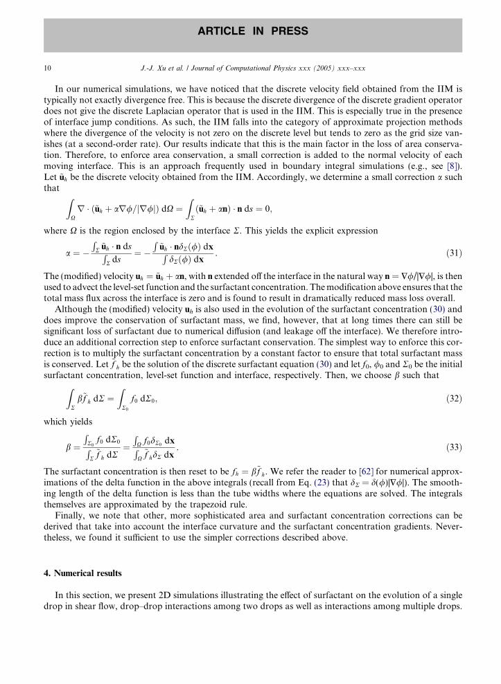
In Fig. 1c, the corresponding capillary (left column) and the Marangoni forces (right column) are plottedas a function of arclength for the different cases. The Capillary force is defined as �rj/Ca and the Marang-oni force is $sr Æ s/Ca (s is the tangential direction) which are calculated on the Cartesian mesh and ob-tained by cubic interpolation at the control points.

The capillary force is largest in magnitude at the drop tips due to the high curvature. At the tips, theforce is negative indicating the tendency to drive the drop-tips inward and thus the drop shape to becomemore circular. The magnitude of the capillary force is largely independent of the surfactant coverage; themagnitude at the drop tips is slightly larger for the larger surfactant coverage because the correspondingdrop-tip has a larger curvature.

At the drop tip, the Marangoni force is zero due to symmetry. Near the drop tips, the Marangoni forcehas positive and negative peaks that act to resist the surfactant redistribution and accumulation at the droptip. The variation of the Marangoni force increases with increasing surfactant coverage. Nevertheless, nearthe drop-tip, the magnitude of the Marangoni force is more than two orders of magnitude smaller than theCapillary force for x = 0.3.

0 5 10 15

0

0 5 10 15

0

0 5 10 15

0

0 5 10 15

0

0 5 10 15

0

0.2

0 5 10 15

0

0.2

0 5 10 15

0

0.2

0 5 10 15

0

0.2

Fig. 1c. Effect of linear EOS and coverage x on Capillary force (left column) and Marangoni force (right column). Notation, times andparameters as in Fig. 1a.

J.-J. Xu et al. / Journal of Computational Physics xxx (2005) xxx–xxx 13

ARTICLE IN PRESS

Next, we examine the numerical errors associated with these calculations. In Fig. 1d, we present the rel-ative errors in drop area (upper left) and surfactant mass (lower left) together with the area correction a(upper right) and surfactant mass correction b (lower right). The results are shown for the coveragex = 0.1; the results with x = 0.3 are similar. The errors in drop-area and surfactant mass are very small– the errors in area and surfactant mass are approximately 0.01% and 0.001%, respectively. This indicatesthat the area and surfactant mass correction algorithms are very effective. The actual values of a and b � 1are approximately 10�3 and 10�5, respectively.

To test the convergence of the algorithm, we perform a resolution study and focus on the maximum dis-tance from the drop interface to the drop center. The maximum distance is plotted as a function of time forthree resolutions (x = 0.1) in Fig. 1e(left). From these results, an order of convergence is estimated and isshown in Fig. 1e(right). After an initial transient, the order of convergence seems to settle between 3 and 4.

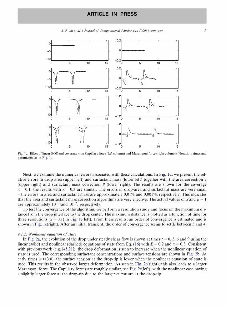
4.1.2. Nonlinear equation of stateIn Fig. 2a, the evolution of the drop under steady shear flow is shown at times t = 0, 3, 6 and 9 using the

linear (solid) and nonlinear (dashed) equations of state from Eq. (16) with E = 0.2 and x = 0.3. Consistentwith previous work (e.g. [45,21]), the drop deformation is seen to increase when the nonlinear equation ofstate is used. The corresponding surfactant concentrations and surface tensions are shown in Fig. 2b. Atearly times (t � 3.0), the surface tension at the drop-tip is lower when the nonlinear equation of state isused. This results in the observed larger deformation. As seen in Fig. 2c(right), this also leads to a largerMarangoni force. The Capillary forces are roughly similar, see Fig. 2c(left), with the nonlinear case havinga slightly larger force at the drop-tip due to the larger curvature at the drop-tip.

0 5 10 15

0

0.5

1x 10

time

rela

tive

area

cha

nge

0 5 10 15

0

5

10x 10

time

α fo

r ar

ea c

orre

ctio

n

0 2 4 6 8 10

0

2

4

6x 10

time

rela

tive

sur

fact

ant m

ass

chan

ge

0 5 10 15

0

2

4

6

8x 10

time

β

Fig. 1d. Relative errors for linear EOS with x = 0.1. All other parameters as in Fig. 1a. Upper left: drop area; lower left: surfactantmass; upper right: area correction a; lower right: surfactant mass correction b.

0 5 10 151

1.5

2

2.5

3

3.5

4

4.5

time

max

imum

dis

tanc

e fr

om in

terf

ace

to c

ente

r

gridsize=800x400 gridsize=400x200 gridsize=200x100

0 2 4 6 80

1

2

3

4

5

6

7

8

9

10

time

conv

erge

nce

rate

for

max

imum

dis

tanc

e

Fig. 1e. Convergence for the maximum distance from the drop-interface to the centroid using linear EOS with x = 0.1. Otherparameters as in Fig. 1a. (Left) maximum distance; (right) order of convergence.

14 J.-J. Xu et al. / Journal of Computational Physics xxx (2005) xxx–xxx

ARTICLE IN PRESS

Fig. 2a. Evolution of drop shape with linear (solid) and nonlinear (dashed) EOS at times t = 0, 3, 6 and 9 with Ca = 0.7, E = 0.2 andx = 0.3.

J.-J. Xu et al. / Journal of Computational Physics xxx (2005) xxx–xxx 15

ARTICLE IN PRESS

4.2. Two drops

We next consider the effect of surfactant on drop–drop interactions in a steady shear flow with Capillarynumber Ca = 0.5. We consider two initially circular drops with radii equal to 1 and with centroids locatedat (�1.7, 0.25) and (1.7, �0.25). The computational domain is [�7, 7] · [�5, 5], the spatial grid size ishx = hy = h = 0.01 and the time step is Dt = h/8.

In Fig. 3a, the drop evolution is shown, at times t = 0, 2, 4, 6, 8 and 10, in the absence of surfactant x = 0(dotted) and with surfactant (solid) where E = 0.2, x = 0.3 and Pe = 10. The surfactant concentration f isinitially uniform and equal to 1. As the drops approach one another, they are deformed by the flow with thesurfactant case being slightly more deformed. As the drops interact, they flatten and a dimple forms in thenear contact region due to lubrication forces. As the drops pass by one another the trailing-edge drop-tipsin the near contact region first flatten and then elongate due to local straining flows that develop as thedrops separate. The separated drops with surfactant are more elongated and rotated than the surfactant-free drops. We note that errors (not shown) in the drop areas and the surfactant masses on each of thedrops are less than 1% throughout the entire simulation.

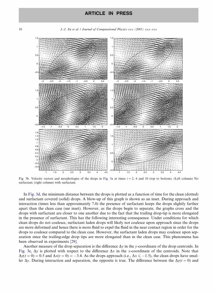
In Fig. 3b, the corresponding (unmodified) velocity vectors relative to the applied shear flow, ~uh � ðy; 0Þ,are shown for the drop with initial centroid located at (�1.7, 0.25). From top to bottom the times are t = 2,6 and 10. The left column corresponds to the case without surfactant. Near the interface at this resolutionthe modified velocity field is identical to the unmodified velocity shown in the figure; this is to be expectedsince the area/velocity correction parameter a is approximately 10�3. The velocity fields with and withoutsurfactant are qualitatively quite similar, however, there are quantitative differences that result in the en-hanced rotation and stretching of the drop with surfactant. The differences are manifest in the structureand location of the two vortices off the drop as well as the velocity near the drop-tips and the drop-centers.

0 5 10 150.5

1

1.5

0 5 10 150

0.5

1

1.5

0 5 10 150

0.5

1

1.5

0 5 10 150

0.5

1

1.5

0 5 10 150.9

1

1.1

0 5 10 150.9

1

1.1

0 5 10 150.9

1

1.1

0 5 10 150.9

1

1.1

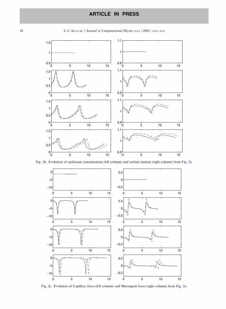
Fig. 2b. Evolution of surfactant concentration (left column) and surface tension (right column) from Fig. 2a.

0 5 10 15

0

0 5 10 15

0

0 5 10 15

0

0 5 10 15

0

0 5 10 15

0

0.2

0 5 10 15

0

0.2

0 5 10 15

0

0.2

0 5 10 15

0

0.2

Fig. 2c. Evolution of Capillary force (left column) and Marangoni force (right column) from Fig. 2a.

16 J.-J. Xu et al. / Journal of Computational Physics xxx (2005) xxx–xxx

ARTICLE IN PRESS

0 2 4 6

0

1

2

3

4

5

t=0

0 2 4 6

0

1

2

3

4

5

t=2

0 2 4 6

0

1

2

3

4

5

t=4

0 2 4 6

0

1

2

3

4

5

t=6

0 2 4 6

0

1

2

3

4

5

t=8

6 0 2 4 6

0

1

2

3

4

5

t=10

Fig. 3a. Morphologies of two drops in shear flow with Ca = 0.5, nonlinear EOS (solid) with E = 0.2, x = 0.3 and Pe = 10. Dotted:x = 0 (no surfactant). Times are t = 0, 2, 4, 6, 8 and 10.

J.-J. Xu et al. / Journal of Computational Physics xxx (2005) xxx–xxx 17

ARTICLE IN PRESS

The evolution of the surfactant concentrations on each drop are shown in Fig. 3c. The left column cor-responds to the drop initially placed at (1.7, �0.25). During approach, the surfactant is swept to the droptips and the distributions are similar to those observed in Section 4.1 for isolated drops. During interaction,surfactant is swept towards the part of the drops in near contact and the concentration near the leading-edge drop-tip is decreased. As the drops begin to separate, a large broad distribution of surfactant is presentalong the flattened drop-tip in the near contact region. Once the drops separate further, the distribution re-focuses as surfactant is again swept towards the elongating drop-tips.

0 0.5

0

0.5

1

1.5

0 0.5

0

0.5

1

1.5

0 0.5 1 1.5 2

0

0.5

1

1.5

0 0.5 1 1.5 2

0

0.5

1

1.5

1 1.5 2 2.5 3 3.5 4 4.5

0

0.2

0.4

0.6

0.8

1

1.2

1.4

1.6

1 1.5 2 2.5 3 3.5 4 4.5

0

0.5

1

1.5

Fig. 3b. Velocity vectors and morphologies of the drops in Fig. 3a at times t = 2, 6 and 10 (top to bottom). (Left column) Nosurfactant; (right column) with surfactant.

18 J.-J. Xu et al. / Journal of Computational Physics xxx (2005) xxx–xxx

ARTICLE IN PRESS

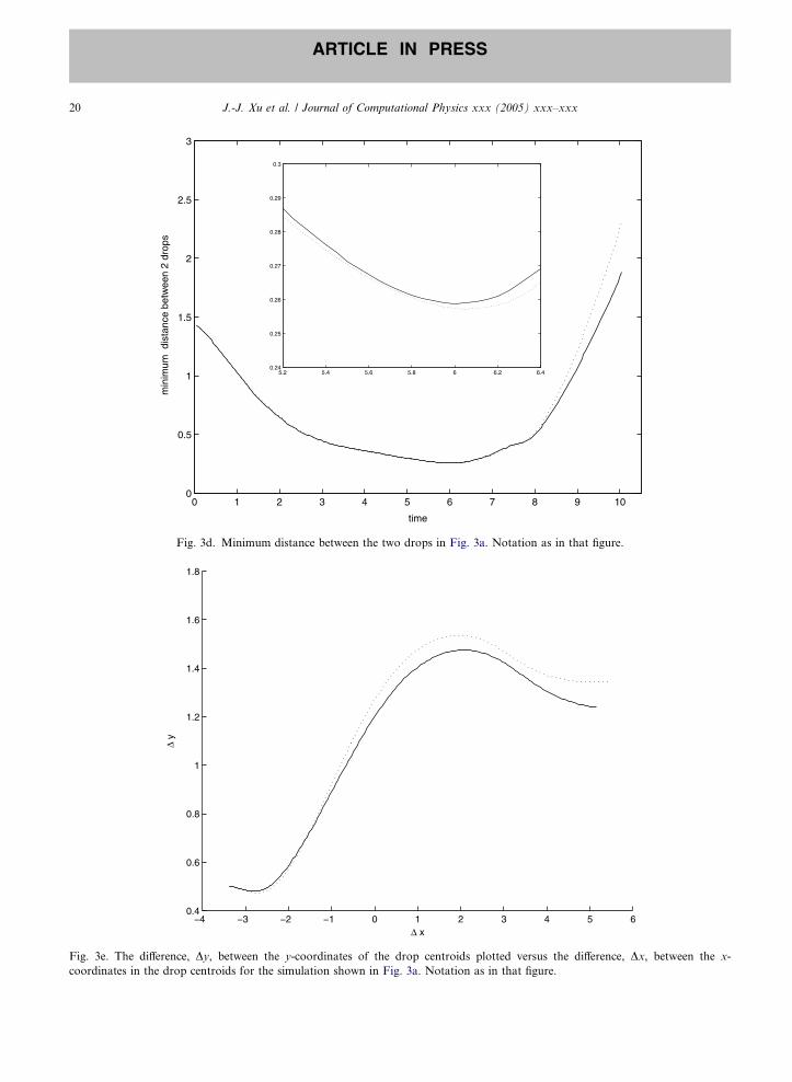
In Fig. 3d, the minimum distance between the drops is plotted as a function of time for the clean (dotted)and surfactant covered (solid) drops. A blow-up of this graph is shown as an inset. During approach andinteraction (times less than approximately 7.0) the presence of surfactant keeps the drops slightly fartherapart than the clean case (see inset). However, as the drops begin to separate, the graphs cross and thedrops with surfactant are closer to one another due to the fact that the trailing drop-tip is more elongatedin the presence of surfactant. This has the following interesting consequence. Under conditions for whichclean drops do not coalesce, surfactant laden drops will likely not coalesce upon approach since the dropsare more deformed and hence there is more fluid to expel the fluid in the near contact region in order for thedrops to coalesce compared to the clean case. However, the surfactant laden drops may coalesce upon sep-aration since the trailing-edge drop tips are more elongated than in the clean case. This phenomena hasbeen observed in experiments [29].

Another measure of the drop separation is the difference Dy in the y-coordinate of the drop centroids. InFig. 3e, Dy is plotted with respect to the difference Dx in the x-coordinate of the centroids. Note thatDy(t = 0) = 0.5 and Dx(t = 0) = �3.4. As the drops approach (i.e., Dx 6 �1.5), the clean drops have smal-ler Dy. During interaction and separation, the opposite is true. The difference between the Dy(t = 0) and

0 2 4 6 8

0.5

1

1.5

2

0 2 4 6 8

0.5

1

1.5

2

0 2 4 6 8

0.5

1

1.5

2

0 2 4 6 8

0.5

1

1.5

2

0 2 4 6 8

0.5

1

1.5

2

0 2 4 6 8

0.5

1

1.5

2

0 2 4 6 8

0.5

1

1.5

2

0 2 4 6 8

0.5

1

1.5

2

0 2 4 6 8

0.5

1

1.5

2

0 2 4 6 8

0.5

1

1.5

2

Fig. 3c. Surfactant concentrations on the drops as a function of arclength from Fig. 3a. (Left) Surfactant concentration from dropinitially located at (1.7, �0.25). (Right) Surfactant concentration from drop initially located at (�1.7, 0.25). Times and parameters as inFig. 3a.

J.-J. Xu et al. / Journal of Computational Physics xxx (2005) xxx–xxx 19

ARTICLE IN PRESS

Dy(tfinal) after interaction and separation is a measure of the so-called hydrodynamic diffusion [39]. That is,through hydrodynamic interactions, drops become more widely spaced than they were initially. This mim-ics the effects of diffusion. From this figure, the presence of surfactants is seen to decrease the hydrodynamicdiffusion compared to the clean case. This is primarily because the surfactant laden drops are more rotatedthan the clean drops. Interestingly, this result suggests that dilute dispersions of drops with surfactant maybe less spread out and may have smaller drop–drop distances than their clean counterparts. Further studiesare being conducted to determine how this result depends on the Capillary number, the surfactant coverageand the initial separation distances.

4.3. Multiple drops

Lastly, we consider the effect of surfactant on systems with four interacting drops in a steady shear flowwith Capillary number Ca = 0.7. Initially, the four drops are circular with radii equal to 1 and with cent-roids (�7.7, 1.05), (�1.7, 0.25), (1.7, �.25) and (7.7, �1.05). The computational domain is [�9, 9] · [�5, 5],the spatial grid size is hx = hy = h = 0.01 and the time step is Dt = h/8.

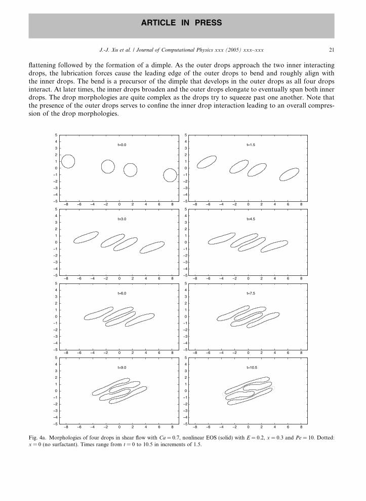
In Fig. 4a, the drop evolution is shown, at times t = 0–10.5 in increments of 1.5. in the absence of sur-factant x = 0 (dotted) and with surfactant (solid) where E = 0.2, x = 0.3 and Pe = 10. The surfactant con-centration f is initially uniform and equal to 1. As in the two-drop case, the four drops are deformed by theflow with the surfactant case being slightly more deformed. The two inner drops interact first leading to

0 1 2 3 4 5 6 7 8 9 100

0.5

1

1.5

2

2.5

3

time

min

imum

dis

tanc

e be

twee

n 2

drop

s

5.2 5.4 5.6 5.8 6 6.2 6.40.24

0.25

0.26

0.27

0.28

0.29

0.3

Fig. 3d. Minimum distance between the two drops in Fig. 3a. Notation as in that figure.

0 1 2 3 4 5 60.4

0.6

0.8

1

1.2

1.4

1.6

1.8

x

y

Fig. 3e. The difference, Dy, between the y-coordinates of the drop centroids plotted versus the difference, Dx, between the x-coordinates in the drop centroids for the simulation shown in Fig. 3a. Notation as in that figure.

20 J.-J. Xu et al. / Journal of Computational Physics xxx (2005) xxx–xxx

ARTICLE IN PRESS

J.-J. Xu et al. / Journal of Computational Physics xxx (2005) xxx–xxx 21

ARTICLE IN PRESS

flattening followed by the formation of a dimple. As the outer drops approach the two inner interactingdrops, the lubrication forces cause the leading edge of the outer drops to bend and roughly align withthe inner drops. The bend is a precursor of the dimple that develops in the outer drops as all four dropsinteract. At later times, the inner drops broaden and the outer drops elongate to eventually span both innerdrops. The drop morphologies are quite complex as the drops try to squeeze past one another. Note thatthe presence of the outer drops serves to confine the inner drop interaction leading to an overall compres-sion of the drop morphologies.

0 2 4 6 8

0

1

2

3

4

5

t=0.0

0 2 4 6 8

0

1

2

3

4

5

t=1.5

0 2 4 6 8

0

1

2

3

4

5

t=3.0

0 2 4 6 8

0

1

2

3

4

5

t=4.5

0 2 4 6 8

0

1

2

3

4

5

t=6.0

0 2 4 6 8

0

1

2

3

4

5

t=7.5

0 2 4 6 8

0

1

2

3

4

5

t=9.0

0 2 4 6 8

0

1

2

3

4

5

t=10.5

Fig. 4a. Morphologies of four drops in shear flow with Ca = 0.7, nonlinear EOS (solid) with E = 0.2, x = 0.3 and Pe = 10. Dotted:x = 0 (no surfactant). Times range from t = 0 to 10.5 in increments of 1.5.

Fig. 4b. Surfactant distribution for the simulation shown in Fig. 4c. Times and parameters as in that figure.

22 J.-J. Xu et al. / Journal of Computational Physics xxx (2005) xxx–xxx

ARTICLE IN PRESS

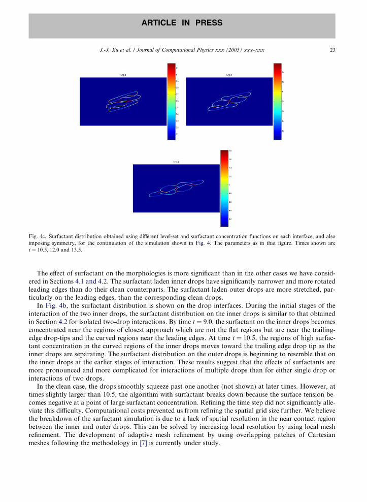
Fig. 4c. Surfactant distribution obtained using different level-set and surfactant concentration functions on each interface, and alsoimposing symmetry, for the continuation of the simulation shown in Fig. 4. The parameters as in that figure. Times shown aret = 10.5, 12.0 and 13.5.

J.-J. Xu et al. / Journal of Computational Physics xxx (2005) xxx–xxx 23

ARTICLE IN PRESS

The effect of surfactant on the morphologies is more significant than in the other cases we have consid-ered in Sections 4.1 and 4.2. The surfactant laden inner drops have significantly narrower and more rotatedleading edges than do their clean counterparts. The surfactant laden outer drops are more stretched, par-ticularly on the leading edges, than the corresponding clean drops.

In Fig. 4b, the surfactant distribution is shown on the drop interfaces. During the initial stages of theinteraction of the two inner drops, the surfactant distribution on the inner drops is similar to that obtainedin Section 4.2 for isolated two-drop interactions. By time t = 9.0, the surfactant on the inner drops becomesconcentrated near the regions of closest approach which are not the flat regions but are near the trailing-edge drop-tips and the curved regions near the leading edges. At time t = 10.5, the regions of high surfac-tant concentration in the curved regions of the inner drops moves toward the trailing edge drop tip as theinner drops are separating. The surfactant distribution on the outer drops is beginning to resemble that onthe inner drops at the earlier stages of interaction. These results suggest that the effects of surfactants aremore pronounced and more complicated for interactions of multiple drops than for either single drop orinteractions of two drops.

In the clean case, the drops smoothly squeeze past one another (not shown) at later times. However, attimes slightly larger than 10.5, the algorithm with surfactant breaks down because the surface tension be-comes negative at a point of large surfactant concentration. Refining the time step did not significantly alle-viate this difficulty. Computational costs prevented us from refining the spatial grid size further. We believethe breakdown of the surfactant simulation is due to a lack of spatial resolution in the near contact regionbetween the inner and outer drops. This can be solved by increasing local resolution by using local meshrefinement. The development of adaptive mesh refinement by using overlapping patches of Cartesianmeshes following the methodology in [7] is currently under study.

24 J.-J. Xu et al. / Journal of Computational Physics xxx (2005) xxx–xxx

ARTICLE IN PRESS

Another possible remedy we are pursuing is the use of different level-set functions and surfactant con-centration functions for each interface. This is discussed further in Section 5 and a preliminary result ofsuch an approach is shown in Fig. 4c. It is known that the use of single surfactant concentration andlevel-set functions to described multiple interfaces may lead to numerical difficulties in extending these func-tions off the interfaces in near contact regions. For example, e.g., see [40], extensions of the level-setfunction off interfaces may lead to poorly behaved discretizations of the interface curvature in regions ofnear contact. Since the discretization of the surfactant equation explicitly uses the interface curvature,see Eq. (30), this can cause the surfactant concentration to become inaccurate. In addition, the extensionof f off the interface may analogously lead to non-smooth derivatives of f which can also lead to inaccuracyin both f and the Marangoni force. We are also studying the use of one-sided differencing of both the level-set function and the surfactant concentration in regions of near contact following the approach developedby Macklin and Lowengrub [40].

5. Conclusions

In this paper, we have presented a level-set method for the simulation of fluid interfaces with insolublesurfactant in two-dimensions. The method can be straightforwardly extended to three-dimensions and tosoluble surfactants. The method couples the IIM for solving the fluid flow equations with a modificationof scheme recently developed by Xu and Zhao [62] for the surfactant transport equation. Novel techniqueswere developed to accurately conserve component (domain) volume and surfactant mass during the evolu-tion. Convergence of the method was demonstrated numerically and the method was applied to study theeffects of surfactant on single drops, drop–drop interactions and interactions among multiple drops inStokes flow under a steady applied shear. Due to Marangoni forces and to non-uniform Capillary forces,the presence of surfactant resulted in larger drop deformations and more complex drop–drop interactionscompared to the analogous cases for clean drops. The effects of surfactant were found to be most significantin flows with multiple drops. To our knowledge, this is the first time that the level-set method has been usedto simulate fluid interfaces with surfactant.

There are a number of future directions that should be pursued. The methods should be extended tothree dimensions and the effect of viscosity ratio on the evolution should be considered. In addition, sur-factant solubility as well as finite Reynolds number flows should also be investigated. From the numericalside, one of the most significant issues to be addressed is increasing the accuracy of interactions amongmany drops in multiphase flows. This is particularly evident from the simulation of four drops in Fig. 4,where the surface tension becomes negative and the simulation breaks down. In this simulation, the com-putational constraints associated with using a uniform Cartesian mesh prevent us from achieving the res-olution required to accurately simulate the drop interactions. To overcome this difficulty, adaptive meshrefinement strategies should be employed.

Another strategy that could be pursued is the use of different level-set and surfactant-concentration func-tions for each interface. That is, instead of using one function to describe the drop morphologies, four level-set functions could be used to describe the fluid morphology. The algorithm presented in this paper couldthen be used to simulate the evolution where the surface forces are obtained by summing the contributionsfrom each drop. Using this strategy, in addition to enforcing symmetry in the flow, we are able to continuethe simulation beyond the previous breakdown time t = 10.5 (in Figs. 4a and 4b) and the result is shown inFig. 4c. However, using this strategy at later times becomes problematic because the drops interact onlythrough the flow. As a result, the drops eventually overlap one another (rather than coalescing) leadingto an unphysical configuration. To overcome this drawback in a general way, hydrodynamic repulsionforces (e.g., lubrication forces) could be introduced to prevent drop overlap. In addition, a locally adaptivemesh should also be used to better resolve the near contact regions. This is currently under study.

J.-J. Xu et al. / Journal of Computational Physics xxx (2005) xxx–xxx 25

ARTICLE IN PRESS

Acknowledgements

The authors thank Mike Siegel and Vittorio Cristini for helpful discussions. The authors acknowledgethe support of the Network and Academic Computing Services at the University of California, Irvine. Theauthors also thank the computing facilities of the Department of Mathematics and the Department of Bio-medical Engineering at the University of California, Irvine. J. Xu acknowledges the support of a PIMS fel-lowship. Z. Li was partially supported by NSF grants DMS-0201094 and DMS-0412654, and by an AROGrant 39676-MA. J. Lowengrub acknowledges the support of the National Science Foundation, Divisionof Mathematical Sciences. H. Zhao is partially supported by an ONR Grant N00014-02-1-0090, a DARPAGrant N00014-02-1-0603 and a Sloan Foundation Fellowship.

References

[1] D. Adalsteinsson, J.A. Sethian, The fast construction of extension velocities in level set methods, J. Comput. Phys. 148 (1999) 2–22.

[2] D. Adalsteinsson, J.A. Sethian, Transport and diffusion of material quantities on propagating interfaces via level set method.Preprint, 2002.

[3] D. Anderson, G. McFadden, A. Wheeler, Diffuse interface methods in fluid mechanics, Ann. Rev. Fluid Mech. 30 (1988) 139.[4] E. Aulisa, S. Manservisi, R. Scardovelli, A mixed markers and volume-of-fluid method for the reconstruction and advection of

interfaces in two-phase and free-boundary flows, J. Comput. Phys. 188 (2003) 611.[5] H.D. Ceniceros, The effects of surfactants on the formation and evolution of capillary waves, Phys. Fluids 15 (2003) 245–256.[6] S. Chen, B. Merriman, S. Osher, P. Smereka, A simple level set method for solving Stefan problems, J. Comput. Phys.

(1997).[7] P. Colella, D.T. Graves, T.J. Ligocki, D.F. Martin, D. Modiano, D.B. Serafini, B. Van Straalen, Chombo Software Package for

AMR Applications, Appl. Num. Alg. Group, NERSC Division, Lawrence Berkeley National Laboratory, Berkeley, CA, 2003.[8] V. Cristini, J. Blawzdziewicz, M. Loewenberg, An adaptive mesh algorithm for evolving surfaces: simulations of drop breakup and

coalescence, J. Comput. Phys. 168 (2001) 445–463.[9] R. Defay, I. Priogine, Surface Tension and Adsorption, Wiley, New York, 1966.[10] M.A. Drumwright-Clarke, Y. Renardy, The effect of insoluble surfactant at dilute concentration on drop breakup under shear

with inertia, Phys. Fluids 16 (2004) 14.[11] C.D. Eggleton, T.-M. Tsai, K.J. Stebe, Tip streaming from a drop in the presence of surfactants, Phys. Rev. Lett. 87 (2001)

048302.[12] D. Enright, R. Fedkiw, J. Ferziger, I. Mitchell, A hybrid particle level set method for improved interface capturing, J. Comput.

Phys. 183 (2002) 83–116.[13] R. Fedkiw, T. Aslam, B. Merriman, S. Osher, A nonoscillary Eulerian approach to interfaces in multimaterials flows (the ghost

fluid method), J. Comput. Phys. 152 (1999) 457–492.[14] F. Gibou, R. Fedkiw, A fourth order accurate discretization for the laplace and heat equations on arbitrary domains with

applications to the Stefan problem, J. Comput. Phys. 202 (2005) 577.[15] J. Glimm, J.W. Grove, X.L. Li, K.-M. Shyue, Q. Zhang, Y. Zeng, Three-dimensional front tracking, SIAM J. Sci. Comput. 19

(1998) 703.[16] J. Goerke, Pulmonary surfactant: functions and molecular composition, Biochim. Biophys. Acta 1408 (1998) 79.[17] B.T. Helenbrook, L. Martinelli, C.K. Law, A numerical method for solving incompressible flow problems with a surface of

discontinuity, J. Comput. Phys. 148 (1999) 366.[18] S.E. Hieber, J.H. Walther, P. Koumoutsakos, Remeshed smoothed particle hydrodynamics simulation of the mechanical behavior

of human organs, Technol. Health Care 12 (2004) 305.[19] T.Y. Hou, Z. Li, S. Osher, H. Zhao, A hybrid method for moving interface problems with applications to the Hele–Shaw flows, J.

Comput. Phys. 134 (1997) 236.[20] T.Y. Hou, J.S. Lowengrub, M.J. Shelley, Boundary integral methods for multicomponent fluids and multiphase materials, J.

Comput. Phys. 169 (2001) 302.[21] A.J. James, J. Lowengrub, A surfactant-conserving volume-of-fluid method for interfacial flows with insoluble surfactant, J.

Comput. Phys. 201 (2004) 685–722.[22] Y.-J. Jan, G. Tryggvason, Computational studies of contaminated bubbles, in: I. Sahin, G. Tryggvason (Eds.), Proceedings of a

Symposium on the Dynamics of Bubbles and Vorticity Near Free Surfaces, vol. 46, ASME, 1991.

26 J.-J. Xu et al. / Journal of Computational Physics xxx (2005) xxx–xxx

ARTICLE IN PRESS

[23] G.-S. Jiang, D. Peng, Weighted eno schemes for Hamilton–Jacobi equations, SIAM J. Sci. Comput. 21 (2000) 2126.[24] G.-S. Jiang, C.-W. Shu, Efficient implementation of weighted ENO schemes, J. Comput. Phys. 126 (1996) 202–228.[25] J.S. Kim, K.K. Kang, J.S. Lowengrub, Conservative multigrid methods for Cahn–Hilliard fluids, J. Comput. Phys. 193 (2004) 511.[26] J.S. Kim, J. Lowengrub, Interfaces and Multicomponent Fluids, Encyclopedia for Math and Physics, Elsevier, to appear, 2005.[27] M. Lai, Z. Li, A remark on jump conditions for the three-dimensional Navier–Stokes equations involving an immersed moving

membrane, Appl. Math. Lett. 14 (2001) 149.[28] L.D. Landau, E.M. Lifshitz, Fluid Mechanics, Pergamon Press, New York, 1958.[29] L.G. Leal, Flow induced coalecsence of drops in a viscous fluid, Phys. Fluids 16 (2004) 1833.[30] L. Lee, R. LeVeque, An immersed interface method for incompressible Navier–Stokes equations, SIAM J. Sci. Comput. 25 (2003)

832.[31] R. LeVeque, Z. Li, The immersed interface method for elliptic equations with discontinuous coefficients and singular sources,

SIAM J. Numer. Anal. 31 (1994) 1019–1044.[32] R. LeVeque, Z. Li, Immersed interface methods for stokes flow with elastic boundaries or surface tension, SIAM.J. Sci. Comput.

18 (1997) 709.[33] X. Li, C. Pozrikidis, Effect of surfactants on drop deformation and on the rheology of dilute emulsion in stokes flow, J. Fluid

Mech. 385 (1999) 79–99.[34] Z. Li, The immersed interface method – a numerical approach for partial differential equations with interfaces. PhD Thesis,

University of Washington, Seattle, 1994.[35] Z. Li, K. Ito, Maximum principle preserving schemes for interface problems with discontinuous coefficients, SIAM J. Sci. Comput.

23 (2001) 339–361.[36] Z. Li, K. Ito, M-C. Lai, An augmented approach for Stokes equations with discontinuous viscosity and singular forces, NCSU

Tech. Reports: CRSC-TR04-24.[37] Z. Li, M. Lai, The immersed interface method for the Navier–Stokes equations with singular forces, J. Comput. Phys. 171 (2001)

822.[38] X. Liu, R. Fedkiw, M. Kang, A boundary condition capturing method for Poisson�s equation on irregular domains, J. Comput.

Phys. 160 (2000) 151.[39] M. Loewenberg, E.J. Hinch, Collision of two deformable drops in shear flow, J. Fluid Mech. 388 (1997) 299.[40] P. Macklin, J. Lowengrub, Evolving interfaces via gradients of geometry-dependent interior Poisson problems: application to

tumor growth, J. Comput. Phys. 203 (2005) 191.[41] W.J. Milliken, H.A. Stone, L.G. Leal, The effect of surfactant on transient motion of Newtonian drops, Phys. Fluids A 5 (1993)

69.[42] N.R. Morrow, G. Mason, Recovery of oil by spontaneous imbibition, Curr. Opin. Coll. Int. Sci. 6 (2001) 321.[43] S. Osher, R.P. Fedkiw, Level set methods: an overview and some recent results, J. Comput. Phys. 169 (2001) 463.[44] S. Osher, J.A. Sethian, Fronts propagating with curvature dependent speed: algorithms based on Hamilton–Jacobi formulations,

J. Comput. Phys. 79 (1988) 12.[45] Y. Pawar, K.J. Stebe, Marangoni effects on drop deformation in an extensional flow: the role of surfactant physical chemistry. I.

Insoluble surfactants, Phys. Fluids 8 (1996) 1738.[46] D. Peng, B. Merriman, S. Osher, H.-K. Zhao, M. Kang, A PDE-based fast local level set method, J. Comput. Phys. 155 (1999)

410.[47] C.S. Peskin, The immersed boundary method, Acta Numer. (2002) 1.[48] C. Pozrikidis, Interfacial dynamics for Stokes flows, J. Comput. Phys. 169 (2001) 250.[49] Y.Y. Renardy, M. Renardy, V. Cristini, A new volume-of-fluid formulation for surfactants and simulations of drop deformation

under shear at a low viscosity ratio, Eur. J. Mech. B 21 (2002) 49–59.[50] R. Scardovelli, S. Zaleski, Direct numerical simulation of free-surface and interfacial flow, Ann. Rev. Fluid Mech. 31 (1999) 567.[51] J.A. Sethian, P. Smereka, Level set methods for fluid interfaces, Ann. Rev. Fluid Mech. 35 (2003) 341.[52] S. Shin, D. Juric, Modeling three-dimensional multiphase flow using a level contour reconstruction method for front tracking

without connectivity, J. Comput. Phys. 180 (2002) 427.[53] C.-W. Shu, Total-variation-diminishing time discretization, SIAM J. Sci. Stat. Comput. 9 (1988) 1073.[54] H.A. Stone, A simple derivation of the time-dependent convective-diffusion equation for surfactant transport along a deforming

interface, Phys. Fluids A 2 (1989) 111.[55] H.A. Stone, L.G. Leal, The effects of surfactants on drop deformation and breakup, J. Fluid Mech. 220 (1990) 161.[56] M. Sussman, A second order coupled level-set and volume-of-fluid method for computing growth and collapse of vapor bubbles,

J. Comput. Phys. 187 (2003) 110.[57] M. Sussman, E. Fatemi, P. Smereka, S. Osher, An improved level set method for incompressible two-phase flows, Comput. Fluids

277 (1998) 663–680.[58] M. Sussman, E. Puckett, A coupled level-set and volume-of-fluid method for computing 3D axisymmetric incompressible two-

phase flows, J. Comput. Phys. 162 (2000) 301.

J.-J. Xu et al. / Journal of Computational Physics xxx (2005) xxx–xxx 27

ARTICLE IN PRESS

[59] M. Sussman, P. Smereka, S. Osher, A level set approach for computing solutions to incompressible two-phase flow, J. Comput.Phys. 114 (1994) 146–159.

[60] G. Tryggvason, B. Bunner, A. Esmaeeli, D. Juric, N. Al-Rawahi, W. Tauber, J. Han, S. Nas, Y.-J. Jan, A front tracking methodfor the computations of multiphase flow, J. Comput. Phys. 169 (2001) 708.

[61] H. Wong, D. Rumschitzki, C. Maldarelli, On the surfactant mass balance at a deforming fluid interface, Phys. Fluids 8 (1996)3203.

[62] J. Xu, H. Zhao, An Eulerian formulation for solving partial differential equations along a moving interface, J. Sci. Comput. 19(2003) 573–594.

[63] S. Yon, C. Pozrikidis, A finite-volume/boundary-element method for flow past interfaces in the presence of surfactants, withapplication to shear flow past a viscous drop, Comput. Fluids 27 (1998) 879.

[64] P. Yue, J.L. Feng, C. Liu, J. Shen, A diffuse-interface method for simulating two-phase flows of complex fluids, J. Fluid Mech. 515(2004) 293.

[65] H. Zhao, T.F. Chan, B. Merriman, S. Osher, A variational level set approach to multiphase motion, J. Comput. Phys. 127 (1996)179–195.