energies

Article

A Large-Eddy Simulation Study of Vertical Axis WindTurbine Wakes in the Atmospheric Boundary Layer

Sina Shamsoddin and Fernando Porté-Agel *

Wind Engineering and Renewable Energy Laboratory (WIRE),École Polytechnique Fédérale de Lausanne (EPFL), EPFL-ENAC-IIE-WIRE, Lausanne 1015, Switzerland;sina.shamsoddin@epfl.ch* Correspondence: fernando.porte-agel@epfl.ch; Tel.: +41-21-693-6138; Fax: +41-21-693-6135

Academic Editor: Frede BlaabjergReceived: 29 March 2016; Accepted: 29 April 2016; Published: 13 May 2016

Abstract: In a future sustainable energy vision, in which diversified conversion of renewable energiesis essential, vertical axis wind turbines (VAWTs) exhibit some potential as a reliable means of windenergy extraction alongside conventional horizontal axis wind turbines (HAWTs). Nevertheless, thereis currently a relative shortage of scientific, academic and technical investigations of VAWTs ascompared to HAWTs. Having this in mind, in this work, we aim to, for the first time, study the wakeof a single VAWT placed in the atmospheric boundary layer using large-eddy simulation (LES). Todo this, we use a previously-validated LES framework in which an actuator line model (ALM) isincorporated. First, for a typical three- and straight-bladed 1-MW VAWT design, the variation ofthe power coefficient with both the chord length of the blades and the tip-speed ratio is analyzedby performing 117 simulations using LES-ALM. The optimum combination of solidity (defined asNc/R, where N is the number of blades, c is the chord length and R is the rotor radius) and tip-speedratio is found to be 0.18 and 4.5, respectively. Subsequently, the wake of a VAWT with these optimumspecifications is thoroughly examined by showing different relevant mean and turbulence wake flowstatistics. It is found that for this case, the maximum velocity deficit at the equator height of theturbine occurs 2.7 rotor diameters downstream of the center of the turbine, and only after that point,the wake starts to recover. Moreover, it is observed that the maximum turbulence intensity (TI) atthe equator height of the turbine occurs at a distance of about 3.8 rotor diameters downstream of theturbine. As we move towards the upper and lower edges of the turbine, the maximum TI (at a certainheight) increases, and its location moves relatively closer to the turbine. Furthermore, whereas bothTI and turbulent momentum flux fields show clear vertical asymmetries (with larger magnitudes atthe upper wake edge compared to the ones at the lower edge), only slight lateral asymmetries wereobserved at the optimum tip-speed ratio for which the simulations were performed.

Keywords: vertical-axis wind turbines (VAWTs); VAWT wake; atmospheric boundary layer (ABL);large-eddy simulation (LES); actuator line model (ALM); turbulence

1. Introduction

Vertical axis wind turbines (VAWTs) offer some advantages over their horizontal axis counterpartsand are being considered as a viable alternative to horizontal axis wind turbines (HAWTs). The researchon VAWT technology started in the 1970s, and while the main focus of the performed studieshas been on the overall turbine performance (quantities such as power and torque) and on themechanical loading on the blades, relatively few studies have attempted to analyze the wake ofa VAWT (for a comprehensive and chronological review of the studies on VAWTs before 2000, seeParaschivoiu [1] (Chapters 4–7)). Having a thorough understanding of VAWT wakes is especiallycrucial in designing VAWT wind farms, where downstream turbines can potentially be located in

Energies 2016, 9, 366; doi:10.3390/en9050366 www.mdpi.com/journal/energies

Energies 2016, 9, 366 2 of 23

the wake of upstream ones, and consequently, the performance of the whole wind farm could besignificantly affected by the wake flow characteristics. Among the experimental works investigatingVAWT wakes, one can find a relatively larger number of studies that have focused only on the nearwake region (e.g., [2–5]), compared to those that have considered also the far wake region (e.g., [6–8]).Nevertheless, from a wind farm design point of view, it is the far wake behavior of the flow that hasmore relevance and importance.

In the numerical flow simulation domain, the studies performed on the flow through VAWTscan be divided into two main categories: (1) the simulations in which the blades of the turbine (andconsequently, the boundary layer around them) are resolved; and (2) the simulations in which theblades are modeled by an actuator-type technique, which uses immersed-body forces to take intoaccount the effects of the blades on the flow. While the first approach (for instance, the work ofCastelli et al. [9]) can be highly valuable to calculate the loading on the blades and the flowcharacteristics inside the rotor and in the near wake, to simulate the far wake of VAWTs and especiallyVAWT wind farms, the second approach is deemed to be more feasible and attainable [10,11]. The useof actuator-type techniques for VAWTs dates back to the 1980s, when Rajagopalan and Fanucci [12]for the first time modeled the VAWT rotor by a porous surface, swept by the blades, on whichtime-averaged blade forces are distributed and continuously act on the flow (which has also beencalled the actuator swept-surface model [11]). An extension of this work to three dimensions wasmade by Rajagopalan et al. [13]. Later on, Shen et al. [14] introduced the actuator surface model andemployed it to obtain the flow field past a VAWT in two dimensions. More recently, Shamsoddin andPorté-Agel [11] used large-eddy simulation (LES) coupled with both the actuator-swept surface model(ASSM) and the actuator line model (ALM) to simulate the flow through a VAWT placed in a waterchannel and compared the resulting wake profiles with experimental data.

Acknowledging the fact that any given real VAWT is likely to be working in the atmosphericboundary layer (ABL) and benefiting from the helpful experience gained from the extensive researchon HAWT wakes, it is imperative to study in detail the characteristics of the wake of VAWTs placed inboundary layer flows, especially if VAWT farms are to be envisaged as a viable source of power infuture energy outlooks. Having this in mind, the present study is a step in this direction and attemptsto use a previously-validated LES framework, in which an actuator line model is incorporated, toanalyze the wake of a typical straight-bladed VAWT in a relatively long downstream range. Moreover,before the wake study, using the same framework, the power production performance of the VAWTfor different combinations of blade chord lengths and tip-speed ratios is studied to find the optimumcombination for the aforementioned wake analysis. To the best knowledge of the authors, this study isthe first attempt to characterize the wake of a VAWT in ABL using LES.

The LES framework is presented in Section 2, and the numerical setups and techniques aredescribed in Section 3. Next, the results for both the power production parametric study and the wakeanalysis are presented and discussed in Section 4. Finally, a summary of the study is given in Section 5.

2. Large-Eddy Simulation Framework

In the LES framework used for the simulations of this paper, the filtered incompressibleNavier–Stokes equations (for a neutrally-stratified ABL) are solved. These equations can be written inrotational form as:

∂ui∂xi

= 0 (1)

∂ui∂t

+ uj(∂ui∂xj−

∂uj

∂xi) = −∂ p∗

∂xi−

∂τij

∂xj− fi

ρ+ Fpδi1 (2)

where the tilde represents a three-dimensional spatial filtering operation at scale ∆, ui is the filteredvelocity in the i-th direction (with i = 1, 2, 3 corresponding to the streamwise (x), spanwise (y) andvertical (z) directions, respectively), p∗ = p

ρ + 12 uiui is the modified kinematic pressure where p is the

Energies 2016, 9, 366 3 of 23

filtered pressure, τij = uiuj− uiuj is the kinematic subgrid-scale (SGS) stress, fi is a body force (per unitvolume) representing the force exerted by the flow on the turbine blades (observe the minus sign), Fp

is an imposed pressure gradient and ρ is the constant fluid density. In this paper, u, v and w notationsare also used for the u1, u2 and u3 velocity components, respectively. Regarding the parametrization ofthe SGS stresses, in these simulations, the Lagrangian scale-dependent dynamic model [15] is used.

To parameterize the VAWT-induced forces on the flow (i.e., to model the term fi/ρ in Equation (2)),an actuator line model is used. According to the ALM, each blade of the turbine is representedby an actuator line on which the turbine forces, calculated based on the blade-element theory, aredistributed. This method has the advantage of being capable of tracking the rotation of the blades ateach time step. For a detailed explanation of the application of the ALM for VAWTs, the reader canrefer to Shamsoddin and Porté-Agel [11] (Section 2.2).

3. Numerical Setup

In this section, the techniques used to numerically solve Equations (1) and (2), as well as theconfiguration of the performed numerical experiments are presented.

The LES code, which is used to realize the simulations in this study, is a modified version ofthe code described by Albertson and Parlange [16], Porté-Agel et al. [17] and Porté-Agel et al. [18].The computational mesh is a 3D structured one, which has Nx, Ny and Nz nodes in the x, y and zdirections, respectively. The mesh is staggered in the z direction in a way that the layers in which thevertical component of velocity (w) is stored are located halfway between the layers in which all of theother main flow variables (u, v, p) are stored. The first w-nodes are located on the z = 0 plane, whilethe first uvp-nodes are located on the z = ∆z/2 plane.

To compute the spatial derivatives, a Fourier-based pseudospectral scheme is used in thehorizontal directions, and a second-order finite difference method is used in the vertical direction.The governing equations for conservation of momentum are integrated in time with the second-orderAdams–Bashforth scheme.

The pressure term in Equation (2) is not a thermodynamic quantity, and it only serves to havea divergence-free (i.e., incompressible) velocity field. Therefore, by taking the divergence of themomentum Equation (2) and using the continuity Equation (1), we can solve the arising Poissonequation for the modified pressure, p∗, using the spectral method in the horizontal directions andfinite differences in the vertical direction.

The boundary conditions (BCs) in the horizontal directions are mathematically (and implicitlythrough using the spectral method) periodic. For the bottom BC, the instantaneous surface shearstress is calculated using the Monin–Obukhov similarity theory [19] as a function of the localhorizontal velocities at the nearest (to the surface) vertical grid points (z = ∆z/2) (see, for instance,Moeng [20], Stoll and Porté-Agel [21]). For the upper boundary, an impermeable stress-free BC isapplied, i.e., ∂u1/∂z = ∂u2/∂z = u3 = 0.

Since the study of the flow through a single turbine is desired, we need to numerically enforcean inflow BC to practically override the implicitly-imposed periodic BC in the x direction. For thispurpose, a buffer zone upstream of the VAWT is employed to adjust the flow to an undisturbed ABLinflow condition. The inflow field is obtained by saving the instantaneous velocity components ina specific y-z plane in a similar precursory simulation of ABL over a flat terrain (with the same surfaceroughness) with no turbine on it. The use of this technique, i.e., using an inflow boundary conditionin a direction in which the flow variables are discretized using Fourier series, has been shown to besuccessful in the works of Tseng et al. [22], Wu and Porté-Agel [23] and Porté-Agel et al. [24].

To implement the ALM, values of the airfoil’s lift and drag coefficients (CL and CD, respectively)as a function of Reynolds number (Re) and angle of attack (α) (i.e., CL(D) = f (Re, α)) are needed.This information was obtained from the tabulated data provided by Sheldahl and Klimas [25].Moreover, the dynamic stall phenomenon, which is known to have a considerable effect on the

Energies 2016, 9, 366 4 of 23

performance of VAWTs [14,26], is accounted for using the modified MIT model [27]. A detailedexplanation of the implementation of the dynamic stall model is provided in Appendix A.

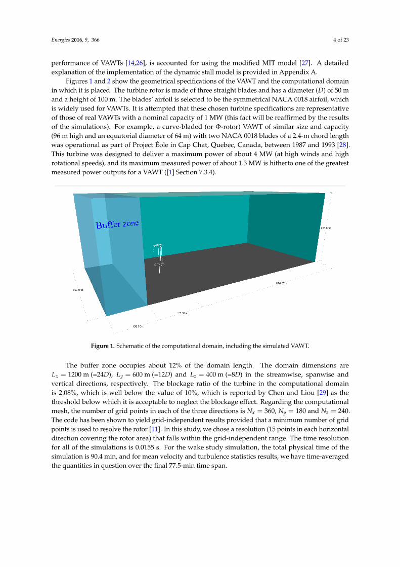
Figures 1 and 2 show the geometrical specifications of the VAWT and the computational domainin which it is placed. The turbine rotor is made of three straight blades and has a diameter (D) of 50 mand a height of 100 m. The blades’ airfoil is selected to be the symmetrical NACA 0018 airfoil, whichis widely used for VAWTs. It is attempted that these chosen turbine specifications are representativeof those of real VAWTs with a nominal capacity of 1 MW (this fact will be reaffirmed by the resultsof the simulations). For example, a curve-bladed (or Φ-rotor) VAWT of similar size and capacity(96 m high and an equatorial diameter of 64 m) with two NACA 0018 blades of a 2.4-m chord lengthwas operational as part of Project Éole in Cap Chat, Quebec, Canada, between 1987 and 1993 [28].This turbine was designed to deliver a maximum power of about 4 MW (at high winds and highrotational speeds), and its maximum measured power of about 1.3 MW is hitherto one of the greatestmeasured power outputs for a VAWT ([1] Section 7.3.4).

Figure 1. Schematic of the computational domain, including the simulated VAWT.

The buffer zone occupies about 12% of the domain length. The domain dimensions areLx = 1200 m (=24D), Ly = 600 m (=12D) and Lz = 400 m (=8D) in the streamwise, spanwise andvertical directions, respectively. The blockage ratio of the turbine in the computational domainis 2.08%, which is well below the value of 10%, which is reported by Chen and Liou [29] as thethreshold below which it is acceptable to neglect the blockage effect. Regarding the computationalmesh, the number of grid points in each of the three directions is Nx = 360, Ny = 180 and Nz = 240.The code has been shown to yield grid-independent results provided that a minimum number of gridpoints is used to resolve the rotor [11]. In this study, we chose a resolution (15 points in each horizontaldirection covering the rotor area) that falls within the grid-independent range. The time resolutionfor all of the simulations is 0.0155 s. For the wake study simulation, the total physical time of thesimulation is 90.4 min, and for mean velocity and turbulence statistics results, we have time-averagedthe quantities in question over the final 77.5-min time span.

Energies 2016, 9, 366 5 of 23

Lx = 1200m = 24D

150m 173.3m

Ly =

60

0m

= 1

2D

30

0m

D = 50m

buffer zone

locus of the VAWT blades

Lz =

40

0m

= 8

D

100m

50m

(a) Top view

(b) Side view (the x-z mid-plane of the domain)

outline of the surface swept by the VAWT blades

x

y

x

z

Figure 2. Plane views of the geometrical configuration of the simulations: (a) top view of the domain;(b) side view of the domain, seen in the x-z mid-plane of the domain.

Figure 3 shows mean and standard deviation profiles of the inflow streamwise velocity.As mentioned earlier, the inflow field is generated by using the flow field of a precursory simulation ofthe neutrally-stratified ABL on a flat terrain. The surface roughness, zo, and the friction velocity, u∗,used in this precursory simulation are 0.1 m and 0.52 m/s, respectively. In Figure 3a, it can be seen thatthe mean streamwise velocity profile approximately follows the log law in the surface layer. The meaninflow streamwise velocity at the equator height of the turbine (i.e., z = 100 m in this case), Ueq, andthe turbulence intensity of the inflow at the same height (σu/Ueq) are 9.6 m/s and 8.3%, respectively.It should be noted that the above-mentioned inflow field is used for all of the simulations of this paper(i.e., both Subsections 4.1 and 4.2).

10−4

10−2

100

5

10

15

20

25

z/Lz

U/u

*

(a)

LES simulation

Log Law

U (m/s)

z (m

)

(b)

0 5 10 150

100

200

300

400

σu/u

*

z (m

)

(c)

0 1 2 30

100

200

300

400

Figure 3. Inflow characteristics: (a) vertical profile of the mean streamwise velocity compared toa log-law profile (horizontal axis in logarithmic scale); (b) vertical profile of the mean streamwisevelocity (linear scale); (c) vertical profile of the standard deviation of the streamwise velocity.

Energies 2016, 9, 366 6 of 23

4. Results and Discussion

In this section, the results of the simulations are presented and discussed. First, we examinethe turbine’s energy-extraction performance, and next, we study the wake flow of a VAWT placed inthe ABL.

4.1. Turbine Performance and Power Extraction

In this subsection, we are interested in how the power production of the turbine is affected bydifferent combinations of tip-speed ratio, TSR, and chord length, c. For this purpose, 117 simulationshave been performed to obtain the power coefficient, CP, of the turbine as a function of both TSRand c, i.e., CP(TSR, c). Figure 4 shows how CP varies with different values of TSR and c. Figure 4ais generated with a resolution of 0.5 m for chord length and 0.5 for TSR. It can be seen that, as weincrease the chord length, the useful TSR range (a range in which CP is higher than a certain value)decreases. Moreover, the figure shows that the maximum power coefficient of the turbine occurs fora TSR of 4.5 and a chord length of 1.5 m (which corresponds to a solidity of Nc/R = 0.18, where Nis the number of blades and R is the rotor radius). This combination results in a power extraction, P,of 1.3 MW and a CP of 0.47 (CP is defined as CP = P/(0.5ρDHUeq

3), where ρ is the fluid density andconsidered equal to 1.225 kg/m3, D is the rotor diameter and H is the rotor height).

TSR

c(m

)

(a)

0.1

0.2

0.3

0.40.4

5

0.45

0.4

0.3

0.2

0.1

0−0.1

−0.2 −

0.3

−0.4

−0.5

−0.6

2 3 4 5 6 7 80.5

1

1.5

2

2.5

3

3.5

4

4.5CP

−0.6

−0.4

−0.2

0

0.2

0.4

TSR

CP

(b)

2 4 6 8−0.4

−0.2

0

0.2

0.4

c = copt = 1.5c = 0.5c = 3c = 4.5

c (m)

CP

(c)

1 2 3 4−0.4

−0.2

0

0.2

0.4

TSR = TSRopt = 4.5

TSR = 3TSR = 6TSR = 8

Figure 4. Variation of the power coefficient of a three-bladed VAWT with tip-speed ratio (TSR) andchord length: (a) CP as a function of both TSR and chord length; (b) CP as a function of TSR for fourdifferent chord lengths; (c) CP as a function of chord length for four different TSR values.

Energies 2016, 9, 366 7 of 23

4.2. VAWT Wake

In this subsection, we have picked the optimum combination of TSR and chord length (TSR = 4.5and c = 1.5 m) for the VAWT rotor and studied the wake flow behind it. Figure 5 shows theinstantaneous streamwise velocity field of the flow in three different orthogonal planes. In all of thefollowing figures in this section containing contour plots, the black circles and rectangles represent theoutline of the locus of the blades. The sense of the rotation of the turbine blades is counterclockwisewhen seen from above. The wake of the VAWT and the highly turbulent nature of the flow are obviousin this figure and in the Videos S1 and S2 included in the Supplementary Material. It should be notedthat the average thrust coefficient of the turbine (defined as CT = T/(0.5ρDHUeq

2), where T is thetotal thrust force of the turbine in the x direction) in this case is found to be 0.8.

x/D

y/D

(a)

−2 0 2 4 6 8 10 12 14 16−6

−4

−2

0

2

4

u/Ueq

0.3

0.4

0.5

0.6

0.7

0.8

0.9

1

1.1

x/D

z/D

(b)

−2 0 2 4 6 8 10 12 14 16

2

4

6

8

u/Ueq

0.2

0.4

0.6

0.8

1

1.2

(c)

y/D

z/D

−6 −4 −2 0 2 4

2

4

6

8

u/Ueq

0.2

0.4

0.6

0.8

1

1.2

Figure 5. Contour plots of the instantaneous normalized streamwise velocity (u/Ueq) in three differentplanes: (a) the x-y plane at the equator height of the turbine; (b) the x-z plane going through the centerof the turbine; (c) the y-z plane which is 2D downstream of the center of the turbine.

Figures 6 and 7 show contour plots of the mean streamwise velocity in the x-y plane at the equatorheight of the turbine and in the x-z mid-plane of the turbine. It can be seen in these figures that it takesa long distance for the wake to recover; at a downwind distance as large as 14 rotor diameters, thewake center velocity reaches only 85% of the incoming velocity. Moreover, Figure 8 shows the meanvelocity contours in six y-z planes downstream of the turbine. In all of these figures (Figures 6–8),one can observe how the wake recovers in the streamwise direction (after a certain distance) and howit expands in the spanwise direction as it advances farther downstream.

Energies 2016, 9, 366 8 of 23

x/D

y/D

−2 0 2 4 6 8 10 12 14 16−6

−4

−2

0

2

4

u/Ueq

0.35

0.4

0.5

0.6

0.7

0.8

0.9

1

Figure 6. Contours of the normalized mean streamwise velocity (u/Ueq) in the x-y plane at the equatorheight of the turbine.

x/D

z/D

−2 0 2 4 6 8 10 12 14 16

2

4

6

8

u/Ueq

0.3

0.6

0.9

1.2

Figure 7. Contours of the normalized mean streamwise velocity (u/Ueq) in the x-z plane going throughthe center of the turbine.

x = 1D

y/D

z/D

−5 0 5

2

4

6

8

x = 2D

y/D−5 0 5

2

4

6

8

x = 4D

y/D

−5 0 5

2

4

6

8

u/Ueq

0.3

0.6

0.9

1.2

x = 6D

y/D

z/D

−5 0 5

2

4

6

8

x = 9D

y/D−5 0 5

2

4

6

8

x = 12D

y/D

−5 0 5

2

4

6

8

u/Ueq

0.3

0.6

0.9

1.2

Figure 8. Contour plots of the normalized mean streamwise velocity (u/Ueq) in six different y-z planesat different distances downstream of the center of the turbine.

Energies 2016, 9, 366 9 of 23

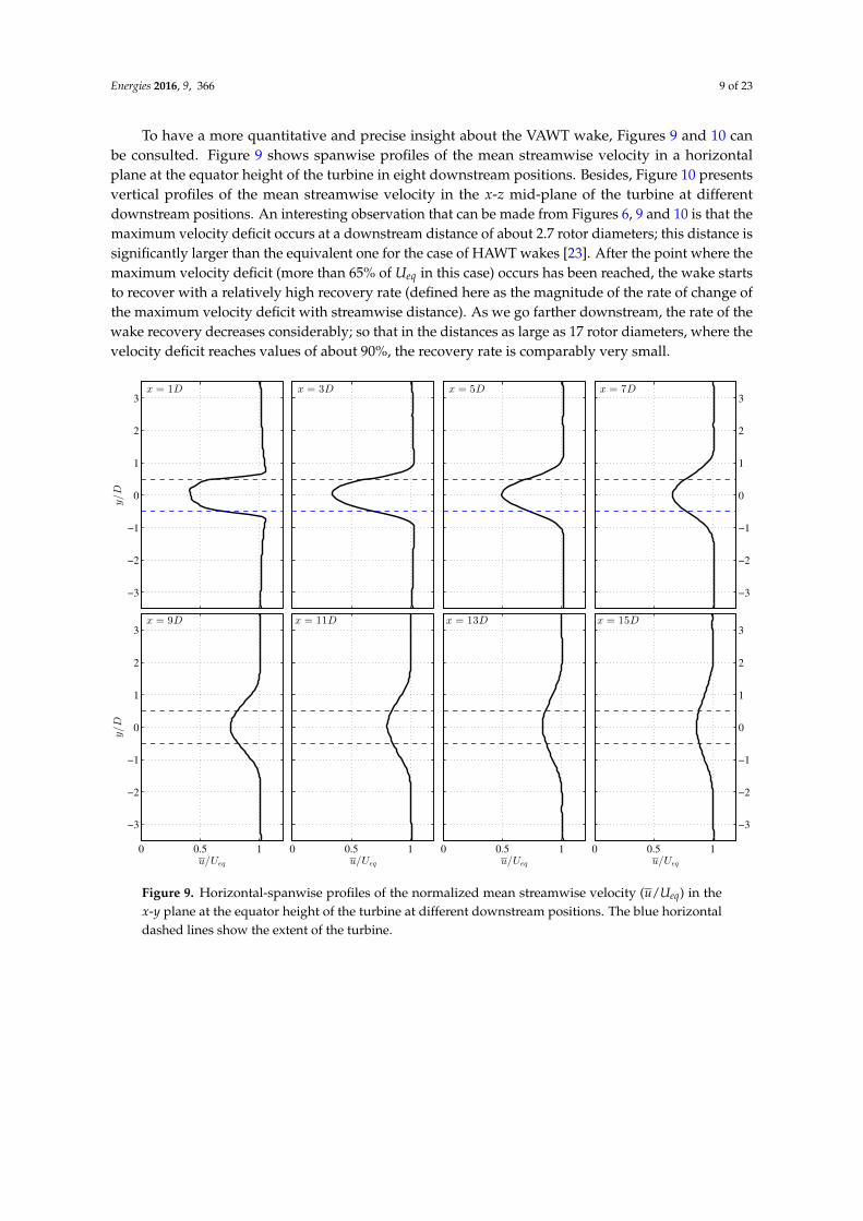
To have a more quantitative and precise insight about the VAWT wake, Figures 9 and 10 canbe consulted. Figure 9 shows spanwise profiles of the mean streamwise velocity in a horizontalplane at the equator height of the turbine in eight downstream positions. Besides, Figure 10 presentsvertical profiles of the mean streamwise velocity in the x-z mid-plane of the turbine at differentdownstream positions. An interesting observation that can be made from Figures 6, 9 and 10 is that themaximum velocity deficit occurs at a downstream distance of about 2.7 rotor diameters; this distance issignificantly larger than the equivalent one for the case of HAWT wakes [23]. After the point where themaximum velocity deficit (more than 65% of Ueq in this case) occurs has been reached, the wake startsto recover with a relatively high recovery rate (defined here as the magnitude of the rate of change ofthe maximum velocity deficit with streamwise distance). As we go farther downstream, the rate of thewake recovery decreases considerably; so that in the distances as large as 17 rotor diameters, where thevelocity deficit reaches values of about 90%, the recovery rate is comparably very small.

x = 1D

y/D

−3

−2

−1

0

1

2

3

x = 3D x = 5D x = 7D

−3

−2

−1

0

1

2

3

x = 9D

u/Ueq

y/D

0 0.5 1

−3

−2

−1

0

1

2

3

x = 11D

u/Ueq

0 0.5 1

x = 13D

u/Ueq

0 0.5 1

x = 15D

u/Ueq

0 0.5 1

−3

−2

−1

0

1

2

3

Figure 9. Horizontal-spanwise profiles of the normalized mean streamwise velocity (u/Ueq) in thex-y plane at the equator height of the turbine at different downstream positions. The blue horizontaldashed lines show the extent of the turbine.

Energies 2016, 9, 366 10 of 23

x = 1D

z/D

0

1

2

3

4

5

6x = 3D x = 5D x = 7D

0

1

2

3

4

5

6

x = 9D

u/Ueq

z/D

0 0.5 10

1

2

3

4

5

x = 11D

u/Ueq

0 0.5 1

x = 13D

u/Ueq

0 0.5 1

x = 15D

u/Ueq

0 0.5 10

1

2

3

4

5

Figure 10. Vertical profiles of the normalized mean streamwise velocity (u/Ueq) in the x-z plane goingthrough the center of the turbine at different downstream positions. The black dashed line representsthe inflow profile, and the blue horizontal dashed lines show the extent of the turbine.

Another group of crucial quantities that has a significant importance in characterizing turbinewakes is the turbulence-related statistics, such as turbulence intensity and turbulent fluxes.These quantities are especially important for the design of wind farms, due to their role in bothwake recovery and mechanical loads on turbine blades. Figure 11 shows contours of turbulenceintensity (TI) in two different orthogonal planes (x-y and x-z) in the wake of the turbine. Here, theturbulence intensity is defined as TI = σu/Ueq. In addition, Figure 12 shows the distribution of TI iny-z planes at different downstream locations. In Figure 11a, it can be seen that two branches of high TIregions start to develop from the two spanwise extremities of the rotor swept surface (the black circle inthe figure). These two branches grow in spanwise width as we go further downstream, until the pointwhere they meet each other (for this case, in about 3.5 rotor diameters downstream of the turbine in thehorizontal mid-plane of the turbine). Starting from the turbine area, the TI in each of these branchesincreases, until a point where the maximum TI occurs (about 3.8 rotor diameters downstream in thiscase); after this maximum point, the TI starts to decrease as the flow advances downstream, while thewidth of the branches continues to expand. Figure 13 examines the previous figure quantitatively, byshowing the spanwise profiles of the TI in the equator height of the turbine. One can readily see thatat each downstream position, the horizontal TI profiles have two maxima at two spanwise positions,which correspond to the two aforementioned TI branches. Although slight asymmetries can stillbe seen in the TI values of the two branches, the lateral asymmetry is not significantly pronounced.It should be noted that the degree to which the VAWT wake is laterally asymmetric is influenced byparameters, such as TSR, airfoil type and the Reynolds number in which the turbine is working.

Energies 2016, 9, 366 11 of 23

x/D

y/D

(a)

−2 0 2 4 6 8 10 12 14 16−6

−4

−2

0

2

4

σu/Ueq

0.1

0.12

0.14

0.16

0.18

0.2

x/D

z/D

(b)

−2 0 2 4 6 8 10 12 14 16

2

4

6

8

σu/Ueq

0.05

0.1

0.15

0.2

Figure 11. Contour plots of the streamwise turbulence intensity, σu/Ueq: (a) in the x-y plane at theequator height of the turbine; (b) in the x-z plane going through the center of the turbine.

1D

y/D

z/D

−5 0 5

2

4

6

8

2D

y/D−5 0 5

2

4

6

8

4D

y/D

−5 0 5

2

4

6

8

σu/Ueq

0.1

0.15

0.2

6D

y/D

z/D

−5 0 5

2

4

6

8

9D

y/D−5 0 5

2

4

6

8

12D

y/D

−5 0 5

2

4

6

8

σu/Ueq

0.1

0.15

0.2

Figure 12. Contour plots of the streamwise turbulence intensity, σu/Ueq, in six different y-z planes atdifferent distances downstream of the center of the turbine.

Energies 2016, 9, 366 12 of 23

x = 1D

y/D

−3

−2

−1

0

1

2

3

x = 3D x = 5D x = 7D

−3

−2

−1

0

1

2

3

x = 9D

σu/Ueq

y/D

0 0.1 0.2

−3

−2

−1

0

1

2

3

x = 11D

σu/Ueq

0 0.1 0.2

x = 13D

σu/Ueq

0 0.1 0.2

x = 15D

σu/Ueq

0 0.1 0.2

−3

−2

−1

0

1

2

3

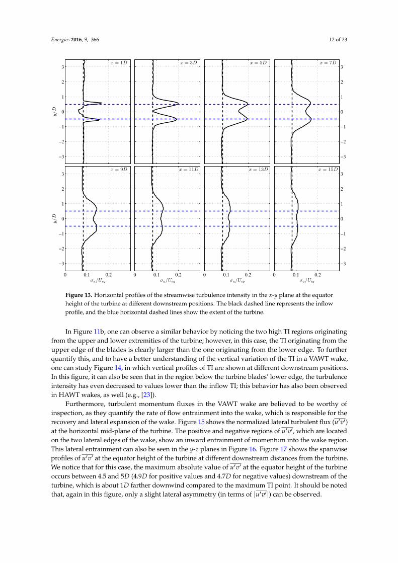
Figure 13. Horizontal profiles of the streamwise turbulence intensity in the x-y plane at the equatorheight of the turbine at different downstream positions. The black dashed line represents the inflowprofile, and the blue horizontal dashed lines show the extent of the turbine.

In Figure 11b, one can observe a similar behavior by noticing the two high TI regions originatingfrom the upper and lower extremities of the turbine; however, in this case, the TI originating from theupper edge of the blades is clearly larger than the one originating from the lower edge. To furtherquantify this, and to have a better understanding of the vertical variation of the TI in a VAWT wake,one can study Figure 14, in which vertical profiles of TI are shown at different downstream positions.In this figure, it can also be seen that in the region below the turbine blades’ lower edge, the turbulenceintensity has even decreased to values lower than the inflow TI; this behavior has also been observedin HAWT wakes, as well (e.g., [23]).

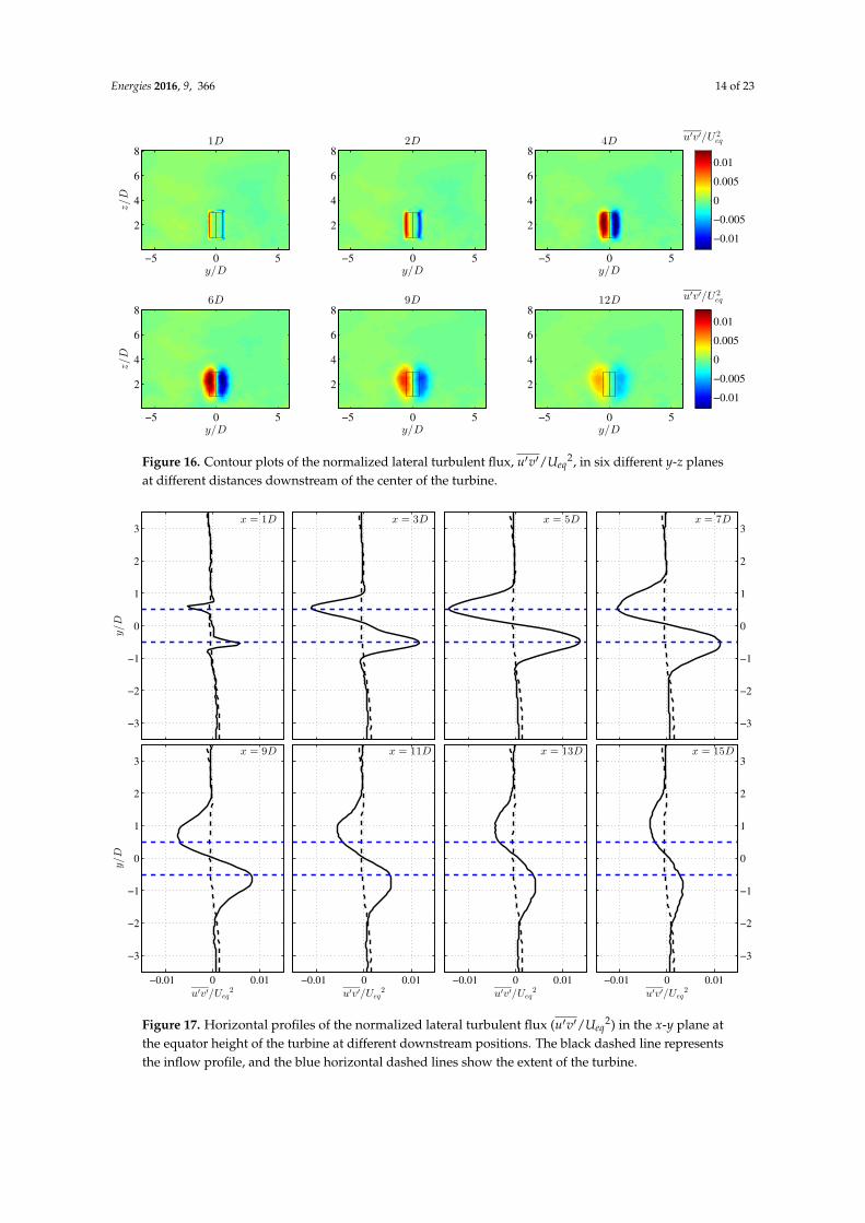
Furthermore, turbulent momentum fluxes in the VAWT wake are believed to be worthy ofinspection, as they quantify the rate of flow entrainment into the wake, which is responsible for therecovery and lateral expansion of the wake. Figure 15 shows the normalized lateral turbulent flux (u′v′)at the horizontal mid-plane of the turbine. The positive and negative regions of u′v′, which are locatedon the two lateral edges of the wake, show an inward entrainment of momentum into the wake region.This lateral entrainment can also be seen in the y-z planes in Figure 16. Figure 17 shows the spanwiseprofiles of u′v′ at the equator height of the turbine at different downstream distances from the turbine.We notice that for this case, the maximum absolute value of u′v′ at the equator height of the turbineoccurs between 4.5 and 5D (4.9D for positive values and 4.7D for negative values) downstream of theturbine, which is about 1D farther downwind compared to the maximum TI point. It should be notedthat, again in this figure, only a slight lateral asymmetry (in terms of |u′v′|) can be observed.

Energies 2016, 9, 366 13 of 23

x = 1D

z/D

0

1

2

3

4

5

6x = 3D x = 5D x = 7D

0

1

2

3

4

5

6

x = 9D

σu/Ueq

z/D

0 0.1 0.20

1

2

3

4

5

x = 11D

σu/Ueq

0 0.1 0.2

x = 13D

σu/Ueq

0 0.1 0.2

x = 15D

σu/Ueq

0 0.1 0.20

1

2

3

4

5

Figure 14. Vertical profiles of the streamwise turbulence intensity in the x-z plane going through thecenter of the turbine at different downstream positions. The black dashed line represents the inflowprofile, and the blue horizontal dashed lines show the extent of the turbine.

x/D

y/D

−2 0 2 4 6 8 10 12 14 16−6

−4

−2

0

2

4

u′v′/Ueq2

−0.01

−0.005

0

0.005

0.01

Figure 15. Contour plot of the normalized lateral turbulent flux, u′v′/Ueq2, in the x-y plane at the

equator height of the turbine.

Energies 2016, 9, 366 14 of 23

1D

y/D

z/D

−5 0 5

2

4

6

8

2D

y/D−5 0 5

2

4

6

8

4D

y/D

−5 0 5

2

4

6

8

u′v′/U 2eq

−0.01

−0.005

0

0.005

0.01

6D

y/D

z/D

−5 0 5

2

4

6

8

9D

y/D−5 0 5

2

4

6

8

12D

y/D

−5 0 5

2

4

6

8

u′v′/U 2eq

−0.01

−0.005

0

0.005

0.01

Figure 16. Contour plots of the normalized lateral turbulent flux, u′v′/Ueq2, in six different y-z planes

at different distances downstream of the center of the turbine.

x = 1D

y/D

−3

−2

−1

0

1

2

3

x = 3D x = 5D x = 7D

−3

−2

−1

0

1

2

3

x = 9D

u′v′/Ueq2

y/D

−0.01 0 0.01

−3

−2

−1

0

1

2

3

x = 11D

u′v′/Ueq2

−0.01 0 0.01

x = 13D

u′v′/Ueq2

−0.01 0 0.01

x = 15D

u′v′/Ueq2

−0.01 0 0.01

−3

−2

−1

0

1

2

3

Figure 17. Horizontal profiles of the normalized lateral turbulent flux (u′v′/Ueq2) in the x-y plane at

the equator height of the turbine at different downstream positions. The black dashed line representsthe inflow profile, and the blue horizontal dashed lines show the extent of the turbine.

Energies 2016, 9, 366 15 of 23

Figures 18 and 19 show the normalized vertical turbulent flux (u′w′) in the wake flow. The verticalinward entrainment from both above and below the wake region is clear in these figures. Figure 20displays the vertical profiles of u′w′ in the x-z plane going through the center of the turbine. It can beseen in this figure that the values of the vertical turbulent flux are higher in upper edge of the wakewith respect to the lower edge. Here, we can observe that the magnitude of u′w′ (in the aforesaidvertical plane) peaks relatively close to the turbine (1.9D for positive values and 0.5D for negativevalues) at heights near to the ones of the upper and lower edges of the blades.

x/D

z/D

−2 0 2 4 6 8 10 12 14 16

2

4

6

8

u′w ′/Ueq2

−0.015

−0.01

−0.005

0

0.005

0.01

0.015

Figure 18. Contour plots of the normalized vertical turbulent flux, u′w′/Ueq2, in the x− z plane going

through the center of the turbine.

1D

y/D

z/D

−5 0 5

2

4

6

8

2D

y/D−5 0 5

2

4

6

8

4D

y/D

−5 0 5

2

4

6

8

u′w ′/Ueq2

−0.01

0

0.01

6D

y/D

z/D

−5 0 5

2

4

6

8

9D

y/D−5 0 5

2

4

6

8

12D

y/D

−5 0 5

2

4

6

8

u′w ′/Ueq2

−0.01

0

0.01

Figure 19. Contour plots of the normalized vertical turbulent flux, u′w′/Ueq2, in six different y-z planes

at different distances downstream of the center of the turbine.

Energies 2016, 9, 366 16 of 23

x = 1Dz/D

0

1

2

3

4

5

6x = 3D x = 5D x = 7D

0

1

2

3

4

5

6

x = 9D

u′w ′/Ueq2

z/D

−0.01 0 0.010

1

2

3

4

5

x = 11D

u′w ′/Ueq2

−0.01 0 0.01

x = 13D

u′w ′/Ueq2

−0.01 0 0.01

x = 15D

u′w ′/Ueq2

−0.01 0 0.010

1

2

3

4

5

Figure 20. Vertical profiles of the normalized vertical turbulent flux (u′w′/Ueq2) in the x-z plane going

through the center of the turbine at different downstream positions. The black dashed line representsthe inflow profile, and the blue horizontal dashed lines show the extent of the turbine.

5. Summary

Acknowledging the prospects of VAWTs as alternative wind energy extractors along with HAWTsin a future clean-energy outlook, which is likely to be marked by diversity, targeted research onVAWTs’ performance is deemed to be highly useful and necessary. One of the research targets, whichis especially crucial in designing potential VAWT farms, is to characterize VAWT wakes; a targetwhich is still considerably underachieved for VAWTs, particularly with respect to HAWTs. In thisview, one of the approaches that can greatly contribute to the cause is to use turbulence-resolvingnumerical simulation techniques, which can provide plenitude of high-resolution spatial and temporalinformation about the flow field and lead to valuable insight into the behavior of the turbine wake.

In this study, we used a previously-validated large-eddy simulation framework, in whichan actuator line model is employed to parameterize the blade forces on the flow, to simulate theatmospheric boundary layer flow through stand-alone VAWTs placed on a flat terrain. For a typicalstraight-bladed 1-MW VAWT rotor design, first, the variation of the power coefficient with the tip-speedratio and the chord length of the blades was studied. In doing so, the optimum combination of TSRand solidity (Nc/R), which yielded the maximum power coefficient of 0.47, was found to be 4.5and 0.18, respectively. Second, for a VAWT with this optimum combination, a detailed study onthe characteristics of its wake was performed, in which different mean and turbulence statisticswere inspected. The mean velocity in the wake was found to need a long distance to recover; forexample, the wake requires a distance of 14 rotor diameters to recover its center velocity to 85% of theincoming velocity. It was also seen that for this case, the point with the maximum velocity deficit islocated 2.7 rotor diameters downstream of the center of the turbine (at the equator height of the turbine),and only after this point, the wake recovery starts with a rate (based on the change of the maximum

Energies 2016, 9, 366 17 of 23

velocity deficit) that is decreasing with streamwise distance. The turbulence intensity was observed toreach its maximum value (at the equator height of the turbine) 3.8 rotor diameters downstream of theVAWT. As we go towards the upper and lower extremities of the rotor, the height-specific maximum ofthe TI moves closer to the turbine and its value also increases. Turbulent momentum fluxes, whichare a gauge for flow entrainment and, as a consequence, are responsible for the recovery of the wake,were also quantified, and it was shown that in the equator height of the turbine, the magnitude ofthe lateral flux peaks about 1D farther downwind of the maximum TI point. The above-mentionedmean and turbulence statistics corresponding to the optimum tip-speed ratio show only slight lateralasymmetries in the wake. However, significant vertical asymmetries were observed in terms of both theTI and magnitude of momentum fluxes, with higher values at the upper edge of the blades comparedto the ones at the lower edge.

This study paves the way to further explore VAWT wakes and to discover the effects of differentrelevant parameters on the wake behavior. Moreover, it can serve as a solid foundation for futurestudies on performance, characteristics and optimization of VAWT farms.

Supplementary Materials: Zenodo DOI:10.5281/zenodo.51387 (https://zenodo.org/record/51387). Video S1:Normalized instantaneous streamwise velocity field both on a vertical plane (x-z) going through the center of theturbine and on a horizontal plane at the equator height of the turbine (Note: the physical time corresponding tothis video is 1 minute and 17 seconds, and the size of the blades is magnified for illustration purposes). Video S2:Normalized instantaneous streamwise velocity field on a horizontal plane at the equator height of the turbine fortwo cases: when the turbine starts to operate (top) and when the flow has reached statistically steady condition(bottom) (Note: the physical time corresponding to both videos is 1 minute and 17 seconds, and the size of theblades is magnified for illustration purposes).

Acknowledgments: This research was supported by EOS (Energie Ouest Suisse) Holding, the Swiss FederalOffice of Energy (Grant SI/501337-01) and the Swiss Innovation and Technology Committee (CTI) within thecontext of the Swiss Competence Center for Energy Research “FURIES: Future Swiss Electrical Infrastructure”.Computing resources were provided by the Swiss National Supercomputing Centre (CSCS) under Project IDss599 and s542.

Author Contributions: This study was done as part of Sina Shamsoddin’s doctoral studies supervised byFernando Porté-Agel.

Conflicts of Interest: The authors declare no conflict of interest.

Appendix A

In this Appendix, the procedure of the method with which the dynamic stall phenomenonis modeled is described in detail. The dynamic stall model is based on the modified MIT modeldeveloped by Noll and Ham [27], which is a practical modification of the original MIT model [30].This model has the advantage of being simple and easy to use and also has been found to work betterfor VAWTs compared to other available models [1]. It is noteworthy that the following procedure canbe implemented for both VAWTs and HAWTs.

Dynamic stall is a phenomenon that occurs for an airfoil when the angle of attack of the incidentflow keeps changing with time and its rate of change (i.e., α = dα

dt ) is sufficiently large. For a bladeelement of a turbine (either VAWT or HAWT) (placed in a turbulent flow), the change of α withtime can be originated by three main sources: (1) the turbulent fluctuations of the incident flow;(2) the changes (spatial or temporal) in the mean incident flow; and (3) the rotation of the blades. Ofthese three reasons, the second one is normally specific to HAWTs, since an HAWT blade elementexperiences the variation of the boundary layer mean velocity profile at different heights; which isnot the case for a VAWT blade element, as it moves at a constant height. However, the third reason isspecific to VAWTs, because the geometry of a VAWT rotor is such that α (for a given blade element)oscillates between a maximum positive value and a minimum negative value in each revolution (evenwith a uniform inflow); however, for an HAWT blade element, assuming a uniform mean inflow, α

remains constant during one revolution. Since the MIT model (and other similar practical models) is(are) only appropriate for the large-scale behavior of α in time, in our implementation of this model,the dynamic stall effects arising from the above-mentioned second and third sources, as well as the

Energies 2016, 9, 366 18 of 23

relatively large-scale turbulent fluctuations (from the first source) are modeled, while the changes of α

arising from the relatively small-scale turbulent fluctuations of the incident flow are filtered out.In order to implement the above-mentioned procedure, α is calculated from a time-averaged and

smoothed curve of α f = α f it(θ) during one revolution. For this purpose, the angle of attack at eachazimuthal angle is time-averaged during each Nrev revolutions of the blades, and then, a polynomialcurve, α f it(θ), is fitted on the time-averaged curve, αavg(θ). For the rest of the dynamic stall calculations,it is the α f it(θ) curve that is used. Figure A1 shows an example for this procedure for TSR = 2 andc = 2 m. The azimuthal angle, θ, is considered to increase counterclockwise (when seen from above)from −90 to 270, in a way that θ = 0 and θ = 180 correspond to the most downstream and themost upstream points of the rotor, respectively. It is also noteworthy to mention again that the senseof the rotation of the turbine blades is counterclockwise when seen from above. Here, for the curvefitting, an eighth order polynomial is used to detect the two extrema accurately.

Azimuthal angle, θ (degree)

An

gle

of

atta

ck, α

(d

egre

e)

−90 0 90 180 270−30

−20

−10

0

10

20

30

αavg

(θ)

αfit

(θ)

α<αSS

Figure A1. The time-averaged (black circles) and curve-fitted (red line) behavior of the variation ofangle of attack as a function of azimuthal angle in one revolution of a blade element.

Subsequently, we implement the modified MIT model on the α f it(θ) curve and construct CL,DS(α)

and CD,DS(α) curves, which are lift and drag coefficients as a function of the angle of attack consideringdynamic stall. In the modified MIT model, we use the tabulated airfoil data for lift and drag coefficients,and based on that, CL,DS(α) and CD,DS(α) are constructed. Based on the tabulated airfoil data, we candetermine the static stall angle, αSS > 0, and the lift coefficient at static stall, CL,SS > 0. The static liftand drag coefficient functions derived from the tabulated airfoil data are designated as CL,table(α) andCD,table(α) hereafter. Moreover, the slope of the CL,table(α) curve before the static stall can be calculatedas as = CL,SS/αSS, considering that in this region, normally, CL,table(α) is linear.

As can be seen in Figure A1, the global (i.e., the curve-fitted) behavior of |α| in one revolution of ablade element is such that |α| twice (once for positive α values and once for negative α values) increasesfrom zero to a maximum value and then decreases to zero again. In each of these increase-decreasecycles of |α|, the MIT dynamic stall model casts the flow in one of the four below dynamic stall states:

State 1 occurs when |α| ≤ αSS. In this state, both lift and drag coefficients are extracteddirectly from the static tabulated airfoil data:

CL,DS(α) = CL,table(|α|) (A1)

CD,DS(α) = CD,table(|α|) (A2)

Energies 2016, 9, 366 19 of 23

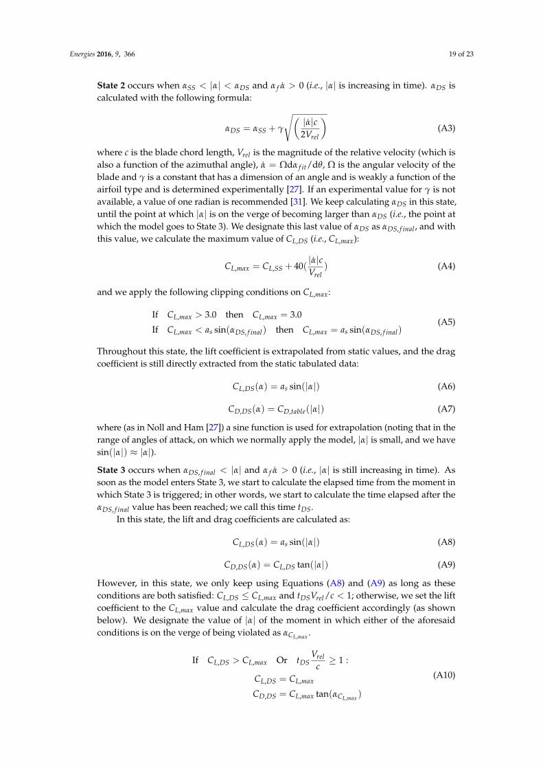
State 2 occurs when αSS < |α| < αDS and α f α > 0 (i.e., |α| is increasing in time). αDS iscalculated with the following formula:

αDS = αSS + γ

√(|α|c2Vrel

)(A3)

where c is the blade chord length, Vrel is the magnitude of the relative velocity (which isalso a function of the azimuthal angle), α = Ωdα f it/dθ, Ω is the angular velocity of theblade and γ is a constant that has a dimension of an angle and is weakly a function of theairfoil type and is determined experimentally [27]. If an experimental value for γ is notavailable, a value of one radian is recommended [31]. We keep calculating αDS in this state,until the point at which |α| is on the verge of becoming larger than αDS (i.e., the point atwhich the model goes to State 3). We designate this last value of αDS as αDS, f inal , and withthis value, we calculate the maximum value of CL,DS (i.e., CL,max):

CL,max = CL,SS + 40(|α|cVrel

) (A4)

and we apply the following clipping conditions on CL,max:

If CL,max > 3.0 then CL,max = 3.0

If CL,max < as sin(αDS, f inal) then CL,max = as sin(αDS, f inal)(A5)

Throughout this state, the lift coefficient is extrapolated from static values, and the dragcoefficient is still directly extracted from the static tabulated data:

CL,DS(α) = as sin(|α|) (A6)

CD,DS(α) = CD,table(|α|) (A7)

where (as in Noll and Ham [27]) a sine function is used for extrapolation (noting that in therange of angles of attack, on which we normally apply the model, |α| is small, and we havesin(|α|) ≈ |α|).

State 3 occurs when αDS, f inal < |α| and α f α > 0 (i.e., |α| is still increasing in time). Assoon as the model enters State 3, we start to calculate the elapsed time from the moment inwhich State 3 is triggered; in other words, we start to calculate the time elapsed after theαDS, f inal value has been reached; we call this time tDS.

In this state, the lift and drag coefficients are calculated as:

CL,DS(α) = as sin(|α|) (A8)

CD,DS(α) = CL,DS tan(|α|) (A9)

However, in this state, we only keep using Equations (A8) and (A9) as long as theseconditions are both satisfied: CL,DS ≤ CL,max and tDSVrel/c < 1; otherwise, we set the liftcoefficient to the CL,max value and calculate the drag coefficient accordingly (as shownbelow). We designate the value of |α| of the moment in which either of the aforesaidconditions is on the verge of being violated as αCL,max .

If CL,DS > CL,max Or tDSVrel

c≥ 1 :

CL,DS = CL,max

CD,DS = CL,max tan(αCL,max )

(A10)

Energies 2016, 9, 366 20 of 23

State 4 occurs when |α| > αSS and α f α ≤ 0 (i.e., when |α| starts to decrease with time).We designate the azimuthal angle of the moment in which |α| starts to decrease as θαmax .At this stage, CL,DS is lowered exponentially (in time) from CL,max to CL,SS.

CL,DS = (CL,max − CL,SS) exp(−(θ − θαmax )

2Rc

)+ CL,SS (A11)

CD,DS(α) = CL,DS tan(|α|) (A12)

where R is the radius of the blade element about the axis of rotation (in the case of a VAWT,R is simply the radius of the VAWT rotor).

As can be noticed in the above procedure, α(t) (i.e., α(θ)) needs to be a smooth function for theabove model to work. Because of this, we use α f = α f it(θ) (i.e., the time-averaged and curve-fittedvalue of α) in the above procedure instead of α. Thus, at the end of each Nrev revolution and aftergetting the α f it(θ) function, we apply the MIT model on this curve, and we construct the CL,DS(α) andCD,DS(α) functions, which will be used in the next Nrev revolutions. For the first Nrev revolutions (forwhich we still do not have α f it(θ)), one can preliminarily just use the static tabulated airfoil data.

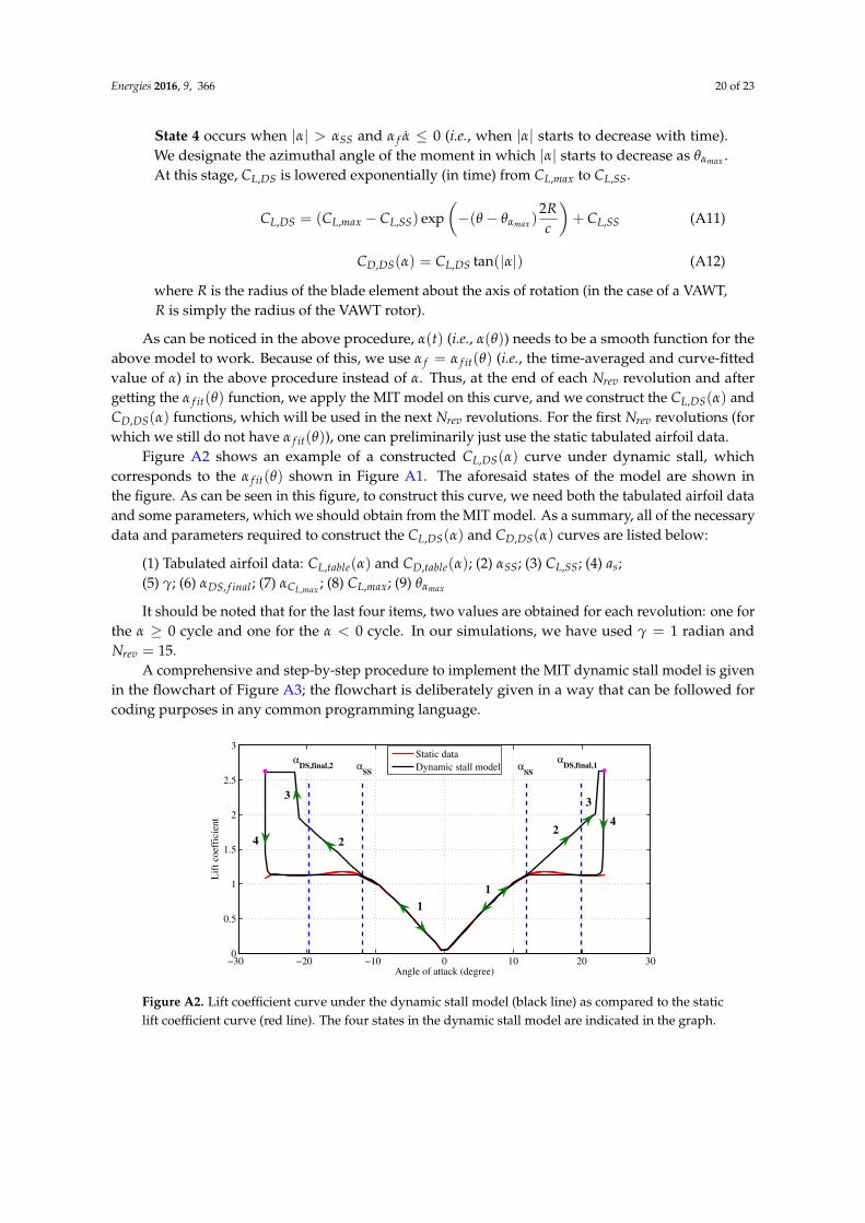
Figure A2 shows an example of a constructed CL,DS(α) curve under dynamic stall, whichcorresponds to the α f it(θ) shown in Figure A1. The aforesaid states of the model are shown inthe figure. As can be seen in this figure, to construct this curve, we need both the tabulated airfoil dataand some parameters, which we should obtain from the MIT model. As a summary, all of the necessarydata and parameters required to construct the CL,DS(α) and CD,DS(α) curves are listed below:

(1) Tabulated airfoil data: CL,table(α) and CD,table(α); (2) αSS; (3) CL,SS; (4) as;(5) γ; (6) αDS, f inal ; (7) αCL,max ; (8) CL,max; (9) θαmax

It should be noted that for the last four items, two values are obtained for each revolution: one forthe α ≥ 0 cycle and one for the α < 0 cycle. In our simulations, we have used γ = 1 radian andNrev = 15.

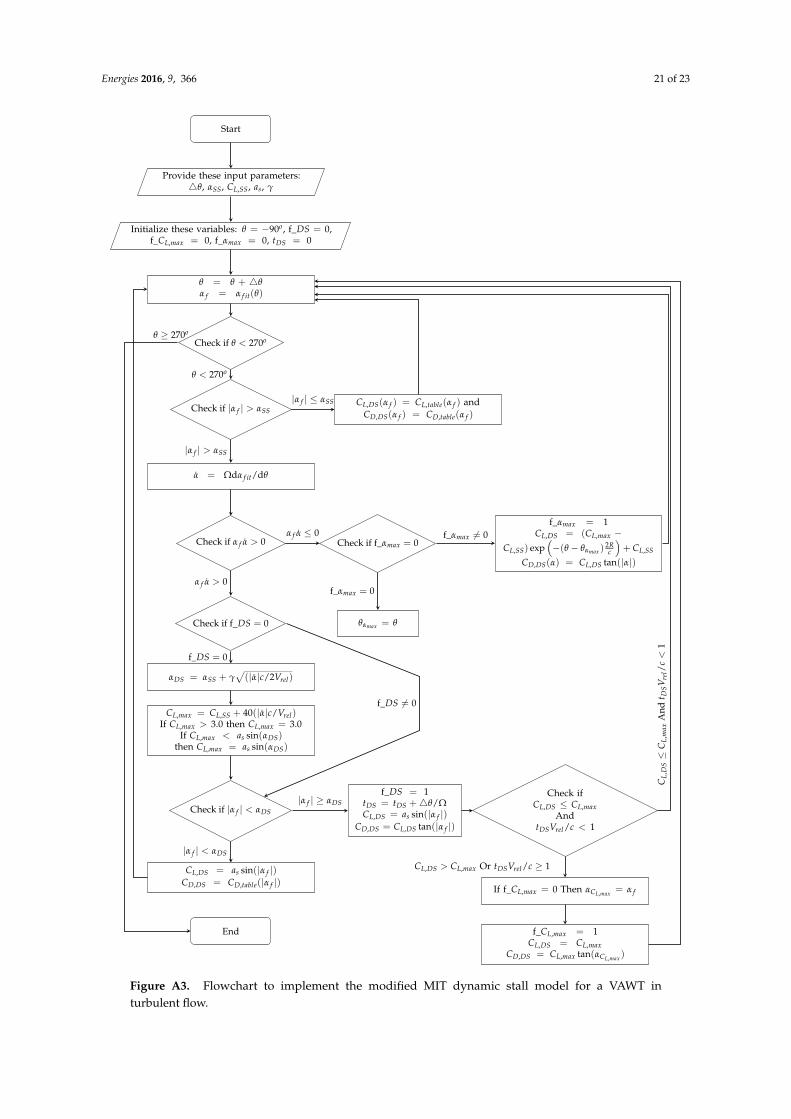
A comprehensive and step-by-step procedure to implement the MIT dynamic stall model is givenin the flowchart of Figure A3; the flowchart is deliberately given in a way that can be followed forcoding purposes in any common programming language.

Angle of attack (degree)

Lif

t co

effi

cien

t

−30 −20 −10 0 10 20 300

0.5

1

1.5

2

2.5

3Static data

Dynamic stall model

3

42

1

24

3

1

αDS,final,2 α

SSα

SS

αDS,final,1

Figure A2. Lift coefficient curve under the dynamic stall model (black line) as compared to the staticlift coefficient curve (red line). The four states in the dynamic stall model are indicated in the graph.

Energies 2016, 9, 366 21 of 23

Start

Provide these input parameters:4θ, αSS, CL,SS, as, γ

Initialize these variables: θ = −90o, f_DS = 0,f_CL,max = 0, f_αmax = 0, tDS = 0

θ = θ + 4θα f = α f it(θ)

Check if θ < 270o

Check if |α f | > αSSCL,DS(α f ) = CL,table(α f ) and

CD,DS(α f ) = CD,table(α f )

α = Ωdα f it/dθ

Check if α f α > 0 Check if f_αmax = 0

θαmax = θ

f_αmax = 1CL,DS = (CL,max −

CL,SS) exp(−(θ − θαmax )

2Rc

)+ CL,SS

CD,DS(α) = CL,DS tan(|α|)

Check if f_DS = 0

αDS = αSS + γ√(|α|c/2Vrel)

CL,max = CL,SS + 40(|α|c/Vrel)If CL,max > 3.0 then CL,max = 3.0

If CL,max < as sin(αDS)then CL,max = as sin(αDS)

Check if |α f | < αDS

f_DS = 1tDS = tDS +4θ/ΩCL,DS = as sin(|α f |)

CD,DS = CL,DS tan(|α f |)

Check ifCL,DS ≤ CL,max

AndtDSVrel/c < 1

If f_CL,max = 0 Then αCL,max = α f

f_CL,max = 1CL,DS = CL,max

CD,DS = CL,max tan(αCL,max )

CL,DS = as sin(|α f |)CD,DS = CD,table(|α f |)

End

θ < 270o

|α f | ≤ αSS

|α f | > αSS

α f α ≤ 0

α f α > 0f_αmax = 0

f_αmax 6= 0

f_DS 6= 0

f_DS = 0

|α f | ≥ αDS

|α f | < αDS

θ ≥ 270o

CL,DS > CL,max Or tDSVrel/c ≥ 1

CL,

DS≤

CL,

max

And

t DSV r

el/

c<

1

Figure A3. Flowchart to implement the modified MIT dynamic stall model for a VAWT inturbulent flow.

Energies 2016, 9, 366 22 of 23

References

1. Paraschivoiu, I. Wind Turbine Design—With Emphasis on Darrieus Concept; Polytechnic International Press:Montreal, QC, Canada, 2002.

2. Tescione, G.; Ragni, D.; He, C.; Simao Ferreira, C.J.; van Bussel, G.J. Experimental and numerical aerodynamicanalysis of vertical axis wind turbine wake. In Proceedings of the International Conference on Aerodynamicsof Offshore Wind Energy Systems and Wakes, Lyngby, Denmark, 17–19 June 2013.

3. Battisti, L.; Zanne, L.; Dell’Anna, S.; Dossena, V.; Persico, G.; Paradiso, B. Aerodynamic measurementson a vertical axis wind turbine in a large scale wind tunnel. J. Energy Resour. Technol. 2011, 133,doi:10.1115/1.4004360.

4. Bachant, P.; Wosnik, M. Characterising the near-wake of a cross-flow turbine. J. Turbul. 2015, 16, 392–410.5. Araya, D.B.; Dabiri, J.O. A comparison of wake measurements in motor-driven and flow-driven turbine

experiments. Exp. Fluids 2015, 56, 1–15.6. Brochier, G.; Fraunie, P.; Beguier, C.; Paraschivoiu, I. Water channel experiments of dynamic stall on darrieus

wind turbine blades. AIAA J. Propuls. Power 1986, 2, 445–449.7. Rolin, V.F.C.; Porté-Agel, F. Wind-tunnel study of the wake behind a vertical axis wind turbine in a boundary

layer flow using stereoscopic particle image velocimetry. J. Phys. Conf. Ser. 2015, 625, 012012.8. Ryan, K.J.; Coletti, F.; Elkins, C.J.; Dabiri, J.O.; Eaton, J.K. Three-dimensional flow field around and

downstream of a subscale model rotating vertical axis wind turbine. Exp. Fluids 2016, 57, 1–15.9. Castelli, M.R.; Englaro, A.; Benini, E. The darrieus wind turbine: Proposal for a new performance prediction

model based on CFD. Energy 2011, 36, 4919–4934.10. Pierce, B.; Moin, P.; Dabiri, J.O. Evaluation of Point-Forcing Models with Application to Vertical Axis Wind

Turbine Farms; Annual Research Briefs; Center for Turbulence Research, Stanford University: Stanford, CA,USA, 2013.

11. Shamsoddin, S.; Porté-Agel, F. Large eddy simulation of vertical axis wind turbine wakes. Energies 2014,7, 890–912.

12. Rajagopalan, R.G.; Fanucci, J.B. Finite difference model for vertical-axis wind turbines. AIAA J. Propuls. Power1985, 1, 432–436.

13. Rajagopalan, R.G.; Berg, D.E.; Klimas, P.C. Development of a three-dimensional model for the darrieus rotorand its wake. AIAA J. Propuls. Power 1995, 11, 185–195.

14. Shen, W.; Zhang, J.; Sørensen, J. The actuator surface model: A new navier-stokes based model for rotorcomputations. J. Sol. Energy Eng. 2009, 131, doi:10.1115/1.3027502.

15. Stoll, R.; Porté-Agel, F. Dynamic subgrid-scale models for momentum and scalar fluxes in large-eddysimulation of neutrally stratified atmospheric boundary layers over heterogeneous terrain. Water Resour. Res.2006, 42, doi:10.1029/2005WR003989.

16. Albertson, J.D.; Parlange, M.B. Surfaces length scales and shear stress: implications for land-atmosphereinteractions over complex terrain. Water Resour. Res. 1999, 35, 2121–2132.

17. Porté-Agel, F.; Meneveau, C.; Parlange, M.B. A scale-dependent dynamic model for large-eddy simulation:Application to a neutral atmospheric boundary layer. J. Fluid Mech. 2000, 415, 261–284.

18. Porté-Agel, F.; Wu, Y.T.; Lu, H.; Conzemius, R.J. Large-eddy simulation of atmospheric boundary layer flowthrough wind turbines and wind farms. J. Wind Eng. Ind. Aerodyn. 2011, 99, 154–168.

19. Monin, A.; Obukhov, M. Basic laws of turbulent mixing in the ground layer of the atmosphere. Tr. Akad.Nauk SSSR Geophiz. Inst. 1954, 24, 163–187.

20. Moeng, C. A large-eddy simulation model for the study of planetary boundary-layer turbulence. J. Atmos. Sci.1984, 46, 2311–2330.

21. Stoll, R.; Porté-Agel, F. Effect of roughness on surface boundary conditions for large-eddy simulation.Bound. Layer Meteorol. 2006, 118, 169–187.

22. Tseng, Y.H.; Meneveau, C.; Parlange, M.B. Modeling flow around bluff bodies and predicting urbandispersion using large eddy simulation. Environ. Sci. Technol. 2006, 40, 2653–2662.

23. Wu, Y.T.; Porté-Agel, F. Large-eddy simulation of wind-turbine wakes: Evaluation of turbineparametrisations. Bound. Layer Meteorol. 2011, 138, 345–366.

24. Porté-Agel, F.; Wu, Y.T.; Chen, C.H. A numerical study of the effects of wind direction on turbine wakes andpower losses in a large wind farm. Energies 2013, 6, 5297–5313.

Energies 2016, 9, 366 23 of 23

25. Sheldahl, R.E.; Klimas, P.C. Aerodynamic Characteristics of Seven Airfoil Sections through 180 Degrees Angle ofAttack for Use in Aerodynamic Analysis of Vertical Axis Wind Turbines; Technical Report SAND80-2114; SandiaNational Laboratories: Albuquerque, NM, USA, 1981.

26. Scheurich, F.; Brown, R. Effect of dynamic stall on the aerodynamics of vertical-axis wind turbines. AIAA J.2011, 49, 2511–2521.

27. Noll, R.B.; Ham, N.D. Dynamic Stall of Small Wind Systems; Technical Report; Aerospace Systems Inc.:Burlington, MA, USA, 1983.

28. Templin, R.J.; Rangi, R.S. Vertical-axis wind turbine development in Canada. IEE Proc. A Phys. Sci. Meas.Instrum. Manag. Educ. Rev. 1983, 130, 555–561.

29. Chen, T.; Liou, L. Blockage corrections in wind tunnel tests of small horizontal-axis wind turbines. Exp. Therm.Fluid Sci. 2011, 35, 565–569.

30. Ham, N.D. Aerodynamic loading on a two-dimensional airfoil during dynamic stall. AIAA J. 1968, 6,1927–1934.

31. Hibbs, B.D. HAWTPerformance with Dynamic Stall; Technical Report SERI/STR 217-2732; AeroVironment,Inc.: Monrovia, CA, USA, 1986.

c© 2016 by the authors; licensee MDPI, Basel, Switzerland. This article is an open accessarticle distributed under the terms and conditions of the Creative Commons Attribution(CC-BY) license (http://creativecommons.org/licenses/by/4.0/).