Y. BazilevsDepartment of Structural Engineering,

University of California–San Diego,

La Jolla, CA 92093

e-mail: yuri@ucsd.edu

A. KorobenkoDepartment of Structural Engineering,

University of California–San Diego,

La Jolla, CA 92093

X. DengDepartment of Structural Engineering,

University of California–San Diego,

La Jolla, CA 92093

J. YanDepartment of Structural Engineering,

University of California–San Diego,

La Jolla, CA 92093

M. KinzelDepartment of Aerospace Engineering,

Division of Engineering and Applied Science,

California Institute of Technology,

Pasadena, CA 91125

J. O. DabiriDepartment of Aerospace Engineering,

Division of Engineering and Applied Science,

California Institute of Technology,

Pasadena, CA 91125

Fluid–Structure InteractionModeling of Vertical-AxisWind TurbinesFull-scale, 3D, time-dependent aerodynamics and fluid–structure interaction (FSI) simu-lations of a Darrieus-type vertical-axis wind turbine (VAWT) are presented. A structuralmodel of the Windspire VAWT (Windspire energy, http://www.windspireenergy.com/) isdeveloped, which makes use of the recently proposed rotation-free Kirchhoff–Love shelland beam/cable formulations. A moving-domain finite-element-based ALE-VMS (arbi-trary Lagrangian–Eulerian-variational-multiscale) formulation is employed for the aero-dynamics in combination with the sliding-interface formulation to handle the VAWTmechanical components in relative motion. The sliding-interface formulation is aug-mented to handle nonstationary cylindrical sliding interfaces, which are needed for theFSI modeling of VAWTs. The computational results presented show good agreement withthe field-test data. Additionally, several scenarios are considered to investigate the tran-sient VAWT response and the issues related to self-starting. [DOI: 10.1115/1.4027466]

1 Introduction

In recent years, the wind-energy industry has been moving intwo main directions: off shore, where energy can be harvestedfrom stronger and more sustained winds, and urban areas, whichare closer to the direct consumer. In the offshore environments,large-size horizontal-axis wind turbines (HAWTs) are at the lead-ing edge. They are equipped with complicated pitch and yaw con-trol mechanisms to keep the turbine in operation for windvelocities of variable magnitude and direction, such as wind gusts.The existing HAWT designs are currently more efficient forlarge-scale power production compared with the VAWT designs.However, smaller-size VAWTs are more suitable for urban envi-ronments and are currently employed for small-scale wind-energygeneration. Nevertheless, wind-energy technologies are maturing,and several studies were recently initiated that involve placingVAWTs off shore [2,3].

There are two main configurations of VAWTs, employing theSavonius or Darrieus rotor types [4]. The Darrieus configurationis a lift-driven turbine. It is more efficient than the Savonius con-figuration, which is a drag-type design. Recently, VAWTs resur-faced as a good source of small-scale electric power for urbanareas. The main reason for this is their compact design. The gener-ator and drive train components are located close to the ground,which allows for easier installation, maintenance, and repair.Another advantage of VAWTs is that they are omidirectional (i.e.,they do not have to be oriented into the main wind direction),which obviates the need to include expensive yaw control

mechanisms in their design. However, this brings up issues relatedto self-starting. The ability of VAWTs to self-start depends on thewind conditions as well as on airfoil designs employed [5]. Stud-ies in Refs. [6,7] reported that a three-bladed H-type Darrieusrotor using a symmetric airfoil is able to self-start. In Ref. [8], theauthor showed that significant atmospheric wind transients arerequired to complete the self-starting process for a fixed-bladeDarieus turbine when it is initially positioned in a dead-bandregion defined as the region with the tip-speed-ratio values thatresult in negative net energy produced per cycle. Self-startingremains an open issue for VAWTs, and an additional starting sys-tem is often required for successful operation.

Due to increased recent emphasis on renewable energy, and, inparticular, wind energy, aerodynamics modeling and simulationof HAWTs in 3D have become a popular research activity [9–17].FSI modeling of HAWTs is less developed, although, recently,several studies were reported showing validation at full-scaleagainst field-test data for medium-size turbines [18], and demon-strating feasibility for application to larger-size offshore wind-turbine designs [10,19]. However, 3D aerodynamics modeling ofVAWTs is lagging behind. The majority of the computations forVAWTs are reported in 2D [20–22], while a recent 3D simulationin Ref. [23] employed a quasi-static representation of the air flowinstead of solving the time-dependent problem. A detailed 3Daerodynamics analysis of a VAWT used for laboratory testing wasrecently performed by some of the authors of the present paper inRef. [24]. The studies included full 3D aerodynamic simulations,validated using experimental data, and a simulation of two side-by-site counter-rotating turbines.

The aerodynamics and FSI computational challenges inVAWTs are different than in HAWTs due to the differences intheir aerodynamic and structural design. Because the rotation axis

Manuscript received March 25, 2014; final manuscript received April 14, 2014;accepted manuscript posted April 22, 2014; published online May 7, 2014. Assoc.Editor: Kenji Takizawa.

Journal of Applied Mechanics AUGUST 2014, Vol. 81 / 081006-1Copyright VC 2014 by ASME

Downloaded From: http://appliedmechanics.asmedigitalcollection.asme.org/ on 07/24/2014 Terms of Use: http://asme.org/terms

is orthogonal to the wind direction, the wind-turbine blades expe-rience rapid and large variations in the angle of attack resulting inan air flow that is constantly switching from being fully attachedto being fully separated. This, in turn, leads to high-frequency andhigh-amplitude variations in the aerodynamic torque acting on therotor, requiring finer mesh resolution and smaller time-step sizefor accurate simulation [24]. VAWT blades are typically long andslender by design. The ratio of cord length to blade height is verylow, requiring finer mesh resolution also in the blade height direc-tion in order to avoid using high-aspect-ratio surface elements,and to better capture turbulent fluctuations in the boundary layer.When the FSI analysis of VAWTs is performed, the simulationcomplexity is further increased. The flexibility in VAWTs doesnot come from the blades, which are practically rigid (althoughblades deform at high rotational speeds), but rather from the toweritself, and its connection to the rotor and ground. As a result, themain FSI challenge is to be able to simulate a spinning rotor thatis mounted on a flexible tower.

In the present paper, we focus on the following developments.We propose a set of techniques that, for the first time, enable FSIsimulations of VAWTs in 3D and at full-scale. We first develop a3D structural model of a Windspire VAWT [1], which makes useof the recently proposed rotation-free Kirchhoff–Love shell andbeam/cable formulations, and their coupling. The model allowsfor the rotor to spin freely and for the tower and blades to undergoelastic deformations. We validate the aerodynamics of the Wind-spire design using the field data reported in Refs. [25–27]. For theFSI computations, to accommodate the spinning rotor and deflect-ing tower and blades, the FSI formulation from Ref. [19] isenhanced to allow the cylindrical sliding interface to also move inspace. Finally, with these new techniques, we perform preliminaryFSI computations in an effort to better understand the self-startingissues.

The paper is outlined as follows. In Sec. 2, we introduce theFSI formulation and present the governing equations of aerody-namics and structural mechanics. We also briefly describe thediscretization techniques employed and the aforementionedenhancement of the sliding-interface formulation. In Sec. 3, weshow the aerodynamic and FSI computations of the WindspireVAWT and discuss start-up issues. In Sec. 4, we draw conclusionsand discuss possible future research directions.

2 Methods for Modeling and Simulation of VAWTs

2.1 Governing Equations at the Continuum Level. To per-form the VAWT simulations, we adopt the FSI framework devel-oped in Ref. [28]. The wind turbine aerodynamics is governed bythe Navier–Stokes equations of incompressible flows. Theincompressible-flow assumption is valid for the present applica-tion because the Mach number is low (� 0:1). The Navier–Stokesequations are posed on a moving spatial domain and are written inthe ALE frame [29] as follows:

q1

@u

@t

����x

þðu� uÞ � $u� f1

� �� $ � r1 ¼ 0 (1)

$ � u ¼ 0 (2)

where q1 is the fluid density, f1 is the external force per unit mass,u and u are velocities of the fluid and fluid mechanics domain,respectively. The stress tensor r1 is defined as

r1 u; pð Þ ¼ �pIþ 2le uð Þ (3)

where p is the pressure, I is the identity tensor, l is the dynamicviscosity, and e uð Þ is the strain-rate tensor given by

e uð Þ ¼ 1

2$uþ $uT� �

(4)

In Eq. (1), jx denotes the time derivative taken with respect to afixed referential domain spatial coordinates x. The spatial deriva-tives in the above equations are taken with respect to the spatialcoordinates x of the current configuration.

The governing equations of structural mechanics written in theLagrangian frame [30] consist of the local balance of linearmomentum, and are given by

q2

d2y

dt2� f2

� �� $ � r2 ¼ 0 (5)

where q2 is the structural density, f2 is the body force per unitmass, r2 is the structural Cauchy stress, and y is the unknownstructural displacement vector.

At the fluid–structure interface, compatibility of the kinematicsand tractions is enforced, namely

u� dy

dt¼ 0 (6)

r1n1 þ r2n2 ¼ 0 (7)

where n1 and n2 are the unit outward normal vectors to the fluidand structural mechanics domain at their interface. Note thatn1 ¼ �n2.

The above equations constitute the basic formulation of the FSIproblem at the continuous level. In what follows, we discuss thediscretization of the above system that is applicable to VAWTmodeling. For a variety of discretization options, FSI couplingstrategies, and applications to a large class of problems in engi-neering, the reader is referred to the recent book on computationalFSI [31].

2.2 Discretization and Special FSI Techniques forVAWTs. The aerodynamics formulation makes use of the FEM-based ALE-VMS approach [29,32,33] augmented with weaklyenforced boundary conditions [34–36]. The former acts as a turbu-lence model, while the latter relaxes the mesh size requirements inthe boundary layer without sacrificing the solution accuracy. ALE-VMS was successfully employed for the aerodynamics simulationof HAWTs and VAWTs in Refs. [9,16,24,37,38], and fluid–structure interaction simulation of HAWTs in Refs. [10,18,19,28].

The structural mechanics of VAWTs are modeled using a com-bination of the recently proposed displacement-based Kirchhoff–Love shell [10,18,39] and beam/cable [40] formulations. Both arediscretized using NURBS-based isogeometric analysis (IGA)[41,42].

The FSI modeling employed here makes use of nonmatchingdiscretization of the interface between the fluid and structure sub-domains. Nonmatching discretizations at the fluid–structure inter-face require the use of interpolation or projection of kinematicand traction data between the nonmatching surface meshes (see,for example, Refs. [28,31,32,43–52]), which is what we do here.

To handle the rotor motion in the aerodynamics problem, thesliding-interface approach is employed. The sliding-interface for-mulation was developed in Ref. [53] to handle flows about objectsin relative motion, and used in the computation of HAWTs in Ref.[16], including FSI coupling [19], and VAWTs in Ref. [24]. Wenote that in application of the FEM to flows with moving mechan-ical components, alternatively to the sliding-interface approach,the Shear–Slip Mesh Update Method [54–56] and its more generalversions [57,58] may also be used to handle objects in relativemotion. A recently developed set of space-time (ST) methods canserve as a third alternative in dealing with objects in relativemotion. The components of this set include the ST/NURBS meshupdate method [17,59,60], ST interface tracking with topologychange [61], and ST computation technique with continuousrepresentation in time [62].

To accommodate the spinning motion of the rotor superposedon the global elastic deformation of the VAWT, and to maintain a

081006-2 / Vol. 81, AUGUST 2014 Transactions of the ASME

Downloaded From: http://appliedmechanics.asmedigitalcollection.asme.org/ on 07/24/2014 Terms of Use: http://asme.org/terms

moving-mesh discretization with good boundary-layer resolutioncritical for aerodynamics accuracy, the sliding-interface techniqueis “upgraded” to handle more complex structural motions. Whileat the fluid–structure interface the fluid mechanics mesh followsthe rotor motion, the outer boundary of the cylindrical domainthat encloses the rotor is only allowed to move as a rigid object.The rigid-body motion part is extracted from the rotor structuralmechanics solution (see, e.g., Ref. [63]) and is applied directly tothe outer boundary of the cylindrical domain enclosing the rotor.The inner boundary of the domain that encloses the cylindricalsubdomain also moves as a rigid object. It follows the motion ofthe cylindrical subdomain, but with the spinning component of themotion removed. The fluid mechanics mesh motion in the interiorof the two subdomains is governed by the equations of elasto-statics with Jacobian-based stiffening [43,57,64–67] to preservethe aerodynamic mesh quality.

3 Computational Results

The computations presented in this section are performed for a1.2 kW Windspire design [1], a three-bladed Darrieus VAWT.The total height of the VAWT tower is 9.0 m and the rotor heightis 6.0 m. The rotor uses the DU06W200 airfoil profile with thechord length of 0.127 m, and is of the Giromill type with straightvertical blade sections attached to the main shaft with horizontalstruts (see Fig. 1). The blades and struts are made of aluminum,and the tower is made of steel. The material parameters andmasses of the main structural components are given in Tables 1and 2.

The VAWT blades and part of the tower that spins with therotor are modeled using Kirchhoff–Love shells, while the strutsand main shaft are modeled as beams. The struts are connected to

the blades, tower shell, and main shaft, which gives a relativelysimple VAWT structural model that can represent the 3D mechan-ics of a spinning, flexible rotor mounted on a flexible tower. SeeFigs. 1(b) and 1(c) for more details of the VAWT geometrydescription. The density of the tower shell is set to be very small(see Table 1) so that most of tower mass is distributed evenlyalong the beam. Quadratic NURBS are employed for both thebeam and shell discretizations. The total number of beam ele-ments is 116, and total number of shell elements is 7029. We notethat all the aerodynamically important surfaces that are “seen” bythe fluid mechanics discretization are modeled using shells.

The aerodynamics and FSI simulations are carried out at realis-tic operating conditions reported in the field-test experiments con-ducted by the National Renewable Energy Laboratory [25] andCaltech Field Laboratory for Optimized Wind Energy [26,27]. Forall cases, the air density and viscosity are set to 1.23 kg/m3 and1:78� 10�5 kg/ms, respectively.

The outer aerodynamics computational domain has the dimen-sions of 50 m, 20 m, and 30 m in the streamwise, vertical, andspanwise directions, respectively, and is shown in Fig. 2. TheVAWT centerline is located 15 m from the inflow and side boun-daries. The radius and height of the inner cylindrical domain thatencloses the rotor are 1.6 m and 7 m, respectively.

At the inflow, a uniform wind velocity profile is prescribed. Onthe top, bottom, and side surfaces of the outer domain no-penetration boundary conditions are prescribed, while zerotraction boundary conditions are set at the outflow.

The aerodynamics mesh has about 8 M elements, which are lin-ear triangular prisms in the blade boundary layers, and linear tetra-hedra elsewhere. The boundary-layer mesh is constructed using18 layers of elements, with the size of the first element in the

Fig. 1 Windspire VAWT structural model with dimensionsincluded: (a) full model using isogeometric NURBS-basedrotation-free shells and beams; (b) model cross section 1 show-ing attachment of the struts to the blades and tower shell; (c)model cross section 2 showing attachment of the struts andtower shell

Table 1 Geometric and material properties of the main VAWTstructural components

Thickness/radius

Young’smodulus

Poisson’sratio Density

Part t/r (mm) E (GPa) � q (kg/m3)

Blades 2/NA 70 0.35 2700Strut 12.7/NA 70 0.35 2700Tower shell 5/44.45 210 0.33 78Tower beam NA/41.08 210 NA 5120.9

Table 2 Masses of the main VAWT structural components

Part Mass (kg)

Blades 26.3Strut 14.1Tower 243.4Total 283.8

Fig. 2 The VAWT aerodynamics computational domain in thereference configuration, including the inner cylindrical region,outer region, and sliding interface that is now allowed to movein space as a rigid object

Journal of Applied Mechanics AUGUST 2014, Vol. 81 / 081006-3

Downloaded From: http://appliedmechanics.asmedigitalcollection.asme.org/ on 07/24/2014 Terms of Use: http://asme.org/terms

wall-normal direction of 0.0003 m, and growth ratio of 1.1. A 2Dslice of the mesh near the rotor is shown in Fig. 3, while Fig. 4shows the zoom on the boundary-layer mesh near one of theblades. The mesh design employed in this simulation is based on arefinement study performed for a Darrieus-type experimental tur-bine in Ref. [24].

All computations are carried out in a parallel computing envi-ronment. The mesh is partitioned into subdomains using METIS[68], and each subdomain is assigned to a compute core. Theparallel implementation of the methodology may be found inRef. [37]. The time-step is set to 1:0� 10�5 s for the aerodynam-ics computation and 2:0� 10�5 s for the FSI analysis.

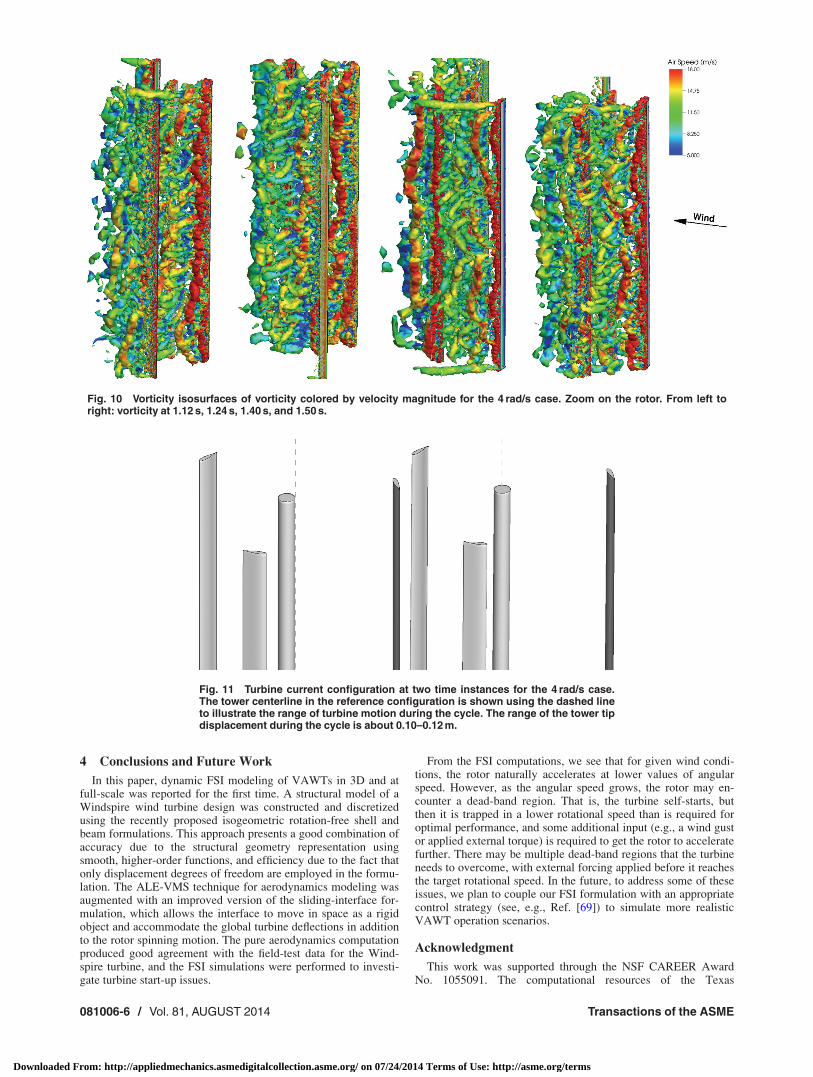
3.1 Aerodynamics Simulation of the Windspire VAWT.We first performed two pure aerodynamic simulations of theWindspire VAWT, one using the wind speed of 8.0 m/s and rotorspeed of 32.7 rad/s, and another using the wind speed of 6.0 m/sand rotor speed of 20.6 rad/s. The time history of the aerodynamictorque for both cases is plotted in Fig. 5 together with the experi-mental values reported from field-test experiments [25–27]. Afterthe rotor undergoes a full revolution, a nearly periodic solution isattained in both cases. For 8.0 m/s wind, the predicted average tor-que is 18.9 Nm, while its experimentally reported value is about12.7 Nm. For 6.0 m/s wind, the predicted average torque is 9.5Nm, while its experimentally reported value is about 4.8 Nm.

In both cases, the experimental value of the aerodynamic torqueis derived from the average power produced by the turbine at thetarget rotor speed. The difference in the predicted and experimen-tally reported aerodynamic torque is likely due to the mechanicaland electrical losses in the system, which are not reported. To esti-mate those, we perform the following analysis. For simplicity, weassume that the torque loss is proportional to the rotational speedof the turbine, that is

Tloss ¼ closs_h (8)

Here, Tloss is taken as the difference between the predicted andreported torque values, _h is the rotation speed, and closs is the“loss” constant that characterizes the turbine. The data for the8.0 m/s wind give closs ¼ 0:19 kg m2/rad, while for 6.0 m/s windwe find that closs ¼ 0:23 kg m2/rad. The two values are reasonablyclose, which suggests that the torque overestimation is consistentwith the loss model. In fact, this technique of combining experi-mental measurements and advanced computation may beemployed to approximately estimate losses in wind turbines.

3.2 FSI Simulations of the Windspire VAWT. In this sec-tion, we perform a preliminary investigation of the start-up issuesin VAWTs using the FSI methodology described earlier and thestructural model of the Windspire design. We fix the inflow windspeed at 11.4 m/s, and consider three initial rotor speeds: 0 rad/s,4 rad/s, and 12 rad/s. Of interest is the transient response of thesystem. In particular, we will focus on how the rotor angularspeed responds to the prescribed initial conditions, and what is therange of the tower tip displacement during the VAWT operation.

The starting configuration of the VAWT is shown in Fig. 3.Blade 1 is placed parallel to the flow with the airfoil leading edgefacing the wind. Blades 2 and 3 are placed at an angle to the flow

Fig. 3 A 2D cross section of the computational mesh along therotor axis. The view is from the top of the turbine, and theblades are numbered counterclockwise, which is the expecteddirection of rotation. The sliding interface may be seen along acircular curve where the mesh appears to be nonconforming.

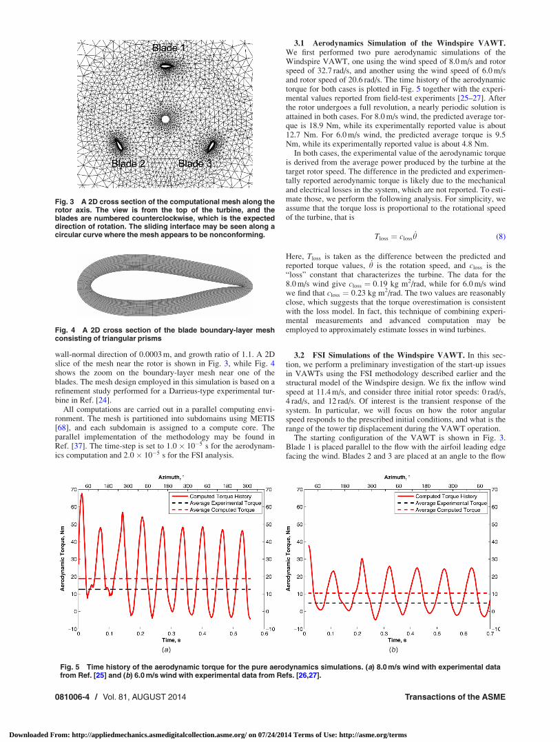
Fig. 4 A 2D cross section of the blade boundary-layer meshconsisting of triangular prisms

Fig. 5 Time history of the aerodynamic torque for the pure aerodynamics simulations. (a) 8.0 m/s wind with experimental datafrom Ref. [25] and (b) 6.0 m/s wind with experimental data from Refs. [26,27].

081006-4 / Vol. 81, AUGUST 2014 Transactions of the ASME

Downloaded From: http://appliedmechanics.asmedigitalcollection.asme.org/ on 07/24/2014 Terms of Use: http://asme.org/terms

with the trailing edge facing the wind. (Blade numbering is shownin the figure.)

The time history of rotor speed is shown in Figs. 6–8. For the0 rad/s case, the rotor speed begins to increase suggesting this con-figuration is favorable for self-starting. For the 4 rad/s case, therotor speed has a nearly linear acceleration region followed by aplateau region. In Ref. [7], the plateau region is defined as the re-gime when the turbine operates at nearly constant (i.e., steady-state like) rotational speed. From the angular position of theblades in Fig. 7, it is evident that the plateau region occurs approx-imately every 120 deg when one of the blades is in a stalled posi-tion. It lasts until the blade clears the stalled region, and the liftforces are sufficiently high for the rotational speed to start

increasing again. As the rotational speed increases, the angular ve-locity is starting to exhibit local unsteady behavior in the plateauregion. While the overall growth of the angular velocity for the4 rad/s case is promising for the VAWT to self-start, the situationis different for the 12 rad/s case (see Fig. 8). Here, the rotor speedhas little dependence on the angular position and stays nearly con-stant, close to its initial value. It is not likely that the rotor speedwill reach to the operational levels in these conditions without anapplied external torque, or a sudden change in wind speed, whichis consistent with the findings of Ref. [8].

Figure 9 shows, for a full turbine, a snapshot of vorticity col-ored by flow speed for the 4 rad/s case. Figure 10 zooms on therotor and shows several flow vorticity snapshots during the rota-tion cycle. The figures indicate the complexity of the underlyingflow phenomena and the associated computational challenges.Note the presence of quasi-2D vortex tubes that are created due tomassive flow separation, and that quickly disintegrate and turninto fine-grained 3D turbulence further downstream. For more dis-cussion on the aerodynamics phenomena involved in VAWTs thereader is referred to Ref. [24].

Figure 11 shows the turbine current configuration at two timeinstances during the cycle for the 4 rad/s case. The displacement ismostly in the direction of the wind, however, lateral tower dis-placements are also observed as a result of the rotor spinningmotion. The displacement amplitude is around 0.10–0.12 m,which is also the case for the 0 rad/s and 12 rad/s cases.

Fig. 6 Time history of the rotor speed starting from 0 rad/s

Fig. 8 Time history of the rotor speed starting from 12 rad/s

Fig. 7 Time history of the rotor speed starting from 4 rad/s

Fig. 9 Vorticity isosurfaces at a time instant colored by veloc-ity magnitude for the 4 rad/s case

Journal of Applied Mechanics AUGUST 2014, Vol. 81 / 081006-5

Downloaded From: http://appliedmechanics.asmedigitalcollection.asme.org/ on 07/24/2014 Terms of Use: http://asme.org/terms

4 Conclusions and Future Work

In this paper, dynamic FSI modeling of VAWTs in 3D and atfull-scale was reported for the first time. A structural model of aWindspire wind turbine design was constructed and discretizedusing the recently proposed isogeometric rotation-free shell andbeam formulations. This approach presents a good combination ofaccuracy due to the structural geometry representation usingsmooth, higher-order functions, and efficiency due to the fact thatonly displacement degrees of freedom are employed in the formu-lation. The ALE-VMS technique for aerodynamics modeling wasaugmented with an improved version of the sliding-interface for-mulation, which allows the interface to move in space as a rigidobject and accommodate the global turbine deflections in additionto the rotor spinning motion. The pure aerodynamics computationproduced good agreement with the field-test data for the Wind-spire turbine, and the FSI simulations were performed to investi-gate turbine start-up issues.

From the FSI computations, we see that for given wind condi-tions, the rotor naturally accelerates at lower values of angularspeed. However, as the angular speed grows, the rotor may en-counter a dead-band region. That is, the turbine self-starts, butthen it is trapped in a lower rotational speed than is required foroptimal performance, and some additional input (e.g., a wind gustor applied external torque) is required to get the rotor to acceleratefurther. There may be multiple dead-band regions that the turbineneeds to overcome, with external forcing applied before it reachesthe target rotational speed. In the future, to address some of theseissues, we plan to couple our FSI formulation with an appropriatecontrol strategy (see, e.g., Ref. [69]) to simulate more realisticVAWT operation scenarios.

Acknowledgment

This work was supported through the NSF CAREER AwardNo. 1055091. The computational resources of the Texas

Fig. 10 Vorticity isosurfaces of vorticity colored by velocity magnitude for the 4 rad/s case. Zoom on the rotor. From left toright: vorticity at 1.12 s, 1.24 s, 1.40 s, and 1.50 s.

Fig. 11 Turbine current configuration at two time instances for the 4 rad/s case.The tower centerline in the reference configuration is shown using the dashed lineto illustrate the range of turbine motion during the cycle. The range of the tower tipdisplacement during the cycle is about 0.10–0.12 m.

081006-6 / Vol. 81, AUGUST 2014 Transactions of the ASME

Downloaded From: http://appliedmechanics.asmedigitalcollection.asme.org/ on 07/24/2014 Terms of Use: http://asme.org/terms

Advanced Computing Center (TACC) [70] were employed for thesimulations reported in this work. This support is gratefullyacknowledged.

References[1] “Windspire Vertical Wind Turbine,” 2014, Ark Alloy, LLC, Reedsburg, WI,

http://www.windspireenergy.com/[2] Vita, L., Paulsen, U. S., and Pedersen, T. F., 2010, “A Novel Floating Offshore

Wind Turbine Concept: New Developments,” European Wind Energy Confer-ence & Exhibition (EWEC 2010), Warsaw, Poland, April 20–23.

[3] Vita, L., Paulsen, U. S., Madsen, H. A., Nielsen, H. P., Berthelsen, P. A., andCartsensen, S., 2012, “Design and Aero-Elastic Simulation of a 5 MW FloatingVertical Axis Wind Turbine,” ASME Paper No. OMAE2012-83470.

[4] Hau, E., 2006, Wind Turbines: Fundamentals, Technologies, Application, Eco-nomics, 2nd ed., Springer, Berlin.

[5] Kirke, B., and Lazauskas, L., 1991, “Enhancing the Performance of a VerticalAxis Wind Turbine Using a Simple Variable Pitch System,” Wind Eng., 15(4),pp. 187–195.

[6] Dominy, R., Lunt, P., Bickerdyke, A., and Dominy, J., 2007, “Self-StartingCapability of a Darrieus Turbine,” Proc. Inst. Mech. Eng., Part A, 221(1),pp. 111–120.

[7] Hill, N., Dominy, R., Ingram, G., and Dominy, J., 2009, “Darrieus Turbines:The Physics of Self-Starting,” Proc. Inst. Mech. Eng., Part A, 223(1),pp. 21–29.

[8] Baker, J. R., 1983, “Features to Aid or Enable Self Starting of Fixed Pitch LowSolidity Vertical Axis Wind Turbines,” J. Wind Eng. Ind. Aerodyn., 15(1–3),pp. 369–380.

[9] Bazilevs, Y., Hsu, M.-C., Akkerman, I., Wright, S., Takizawa, K., Henicke, B.,Spielman, T., and Tezduyar, T. E., 2011, “3D Simulation of Wind TurbineRotors at Full Scale. Part I: Geometry Modeling and Aerodynamics,” Int. J.Numer. Methods Fluids, 65(1–3), pp. 207–235.

[10] Bazilevs, Y., Hsu, M.-C., Kiendl, J., W€uchner, R., and Bletzinger, K.-U., 2011,“3D Simulation of Wind Turbine Rotors at Full Scale. Part II: Fluid–StructureInteraction Modeling With Composite Blades,” Int. J. Numer. Methods Fluids,65(1–3), pp. 236–253.

[11] Chow, R., and van Dam, C. P., 2012, “Verification of Computational Simula-tions of the NREL 5 MW Rotor With a Focus on Inboard Flow Separation,”Wind Energy, 15(8), pp. 967–981.

[12] Bechmann, A., Sørensen, N. N., and Zahle, F., 2011, “CFD Simulations of theMEXICO Rotor,” Wind Energy, 14(5), pp. 677–689.

[13] Takizawa, K., Henicke, B., Tezduyar, T. E., Hsu, M.-C., and Bazilevs, Y.,2011, “Stabilized Space–Time Computation of Wind-Turbine Rotor Aero-dynamics,” Comput. Mech., 48(3), pp. 333–344.

[14] Takizawa, K., Henicke, B., Montes, D., Tezduyar, T. E., Hsu, M.-C., and Bazilevs,Y., 2011, “Numerical-Performance Studies for the Stabilized Space–Time Compu-tation of Wind-Turbine Rotor Aerodynamics,” Comput. Mech., 48(6),pp. 647–657.

[15] Sørensen, N. N., and Schreck, S., 2012, “Computation of the National Renew-able Energy Laboratory Phase-VI Rotor in Pitch Motion During Standstill,”Wind Energy, 15(3), pp. 425–442.

[16] Hsu, M.-C., Akkerman, I., and Bazilevs, Y., 2013, “Finite Element Simulationof Wind Turbine Aerodynamics: Validation Study Using NREL Phase VIExperiment,” Wind Energy, 17(3), pp. 461–481.

[17] Takizawa, K., Tezduyar, T. E., McIntyre, S., Kostov, N., Kolesar, R., andHabluetzel, C., 2014, “Space–Time VMS Computation of Wind-Turbine Rotorand Tower Aerodynamics,” Comput. Mech., 53(1), pp. 1–15.

[18] Korobenko, A., Hsu, M., Akkerman, I., Tippmann, J., and Bazilevs, Y., 2013,“Structural Mechanics Modeling and FSI Simulation of Wind Turbines,” Math.Models Methods Appl. Sci., 23(2), pp. 249–272.

[19] Hsu, M.-C., and Bazilevs, Y., 2012, “Fluid–Structure Interaction Modeling ofWind Turbines: Simulating the Full Machine,” Comput. Mech., 50(6),pp. 821–833.

[20] Stein, P., Hsu, M.-C., Bazilevs, Y., and Beucke, K., 2012, “Operator- andTemplate-Based Modeling of Solid Geometry for Isogeometric Analysis WithApplication to Vertical Axis Wind Turbine Simulation,” Comput. MethodsAppl. Mech. Eng., 213–216, pp. 71–83.

[21] Scheurich, F., Fletcher, T., and Brown, R., 2011, “Simulating the AerodynamicPerformance and Wake Dynamics of a Vertical-Axis Wind Turbine,” WindEnergy, 14(2), pp. 159–177.

[22] Scheurich, F., and Brown, R., 2012, “Modelling the Aerodynamics of Vertical-Axis Wind Turbines in Unsteady Wind Conditions”. Wind Energy., 16(1), pp.91–107.

[23] McLaren, K., Tullis, S., and Ziada, S., 2012, “Computational Fluid DynamicsSimulation of the Aerodynamics of a High Solidity, Small-Scale Vertical AxisWind Turbine,” Wind Energy, 15(3), pp. 349–361.

[24] Korobenko, A., Hsu, M.-C., Akkerman, I., and Bazilevs, Y., 2013,“Aerodynamic Simulation of Vertical-Axis Wind Turbines,” ASME J. Appl.Mech., 81(2), p. 021011.

[25] Huskey, A., Bowen, A., and Jager, D., 2009, “Wind Turbine Generator SystemPower Performance Test Report for the Mariah Windspire 1-kW WindTurbine,” National Renewable Energy Laboratory, Golden, CO, TechnicalReport No. NREL/TP-500-46192.

[26] Dabiri, J. O., 2011, “Potential Order-of-Magnitude Enhancement of Wind FarmPower Density Via Counter-Rotating Vertical-Axis Wind Turbine Arrays,” J.Renewable Sustainable Energy, 3(4), p. 043104.

[27] “Biological Propulsion Laboratory at CALTECH (Wind Energy Research),”2012, California Institute of Technology, Pasadena, CA, http://dabiri.caltech.edu/research/wind-energy.html

[28] Bazilevs, Y., Hsu, M.-C., and Scott, M. A., 2012, “Isogeometric Fluid–Structure Interaction Analysis With Emphasis on Non-Matching Discretiza-tions, and With Application to Wind Turbines,” Comput. Methods Appl. Mech.Eng., 249–252, pp. 28–41.

[29] Hughes, T. J. R., Liu, W. K., and Zimmermann, T. K., 1981,“Lagrangian–Eulerian Finite Element Formulation for Incompressible ViscousFlows,” Comput. Methods Appl. Mech. Eng., 29(3), pp. 329–349.

[30] Belytschko, T., Liu, W. K., and Moran, B., 2000, Nonlinear Finite Elements forContinua and Structures, Wiley, New York.

[31] Bazilevs, Y., Takizawa, K., and Tezduyar, T. E., 2013, Computational Fluid–Structure Interaction: Methods and Applications, Wiley, New York.

[32] Takizawa, K., Bazilevs, Y., and Tezduyar, T. E., 2012, “Space–Time and ALE-VMS Techniques for Patient-Specific Cardiovascular Fluid–Structure Interac-tion Modeling,” Arch. Comput. Methods Eng., 19(2), pp. 171–225.

[33] Bazilevs, Y., Hsu, M.-C., Takizawa, K., and Tezduyar, T. E., 2012, “ALE-VMS and ST-VMS Methods for Computer Modeling of Wind-Turbine RotorAerodynamics and Fluid–Structure Interaction,” Math. Models Methods Appl.Sci., 22(Supp 02), p. 1230002.

[34] Bazilevs, Y., and Hughes, T. J. R., 2007, “Weak Imposition of Dirichlet Bound-ary Conditions in Fluid Mechanics,” Comput. Fluids, 36(1), pp. 12–26.

[35] Bazilevs, Y., Michler, C., Calo, V. M., and Hughes, T. J. R., 2007, “WeakDirichlet Boundary Conditions for Wall-Bounded Turbulent Flows,” Comput.Methods Appl. Mech. Eng., 196(49–52), pp. 4853–4862.

[36] Bazilevs, Y., Michler, C., Calo, V. M., and Hughes, T. J. R., 2010,“Isogeometric Variational Multiscale Modeling of Wall-Bounded TurbulentFlows With Weakly Enforced Boundary Conditions on Unstretched Meshes,”Comput. Methods Appl. Mech. Eng., 199(13–16), pp. 780–790.

[37] Hsu, M.-C., Akkerman, I., and Bazilevs, Y., 2011, “High-Performance Comput-ing of Wind Turbine Aerodynamics Using Isogeometric Analysis,” Comput.Fluids, 49(1), pp. 93–100.

[38] Hsu, M.-C., Akkerman, I., and Bazilevs, Y., 2012, “Wind Turbine Aerodynam-ics Using ALE–VMS: Validation and the Role of Weakly Enforced BoundaryConditions,” Comput. Mech., 50(4), pp. 499–511.

[39] Kiendl, J., Bletzinger, K.-U., Linhard, J., and W€uchner, R., 2009, “IsogeometricShell Analysis With Kirchhoff–Love Elements,” Comput. Methods Appl.Mech. Eng., 198(49–52), pp. 3902–3914.

[40] Raknes, S., Deng, X., Bazilevs, Y., Benson, D., Mathisen, K., and Kvamsdal,T., 2013, “Isogeometric Rotation-Free Bending-Stabilized Cables: Statics, Dy-namics, Bending Strips and Coupling With Shells,” Comput. Methods Appl.Mech. Eng., 263, pp. 127–143.

[41] Hughes, T. J. R., Cottrell, J. A., and Bazilevs, Y., 2005, “Isogeometric Analysis:CAD, Finite Elements, NURBS, Exact Geometry, and Mesh Refinement,”Comput. Methods Appl. Mech. Eng., 194(39–41), pp. 4135–4195.

[42] Cottrell, J. A., Hughes, T. J. R., and Bazilevs, Y., 2009, Isogeometric Analysis:Toward Integration of CAD and FEA, Wiley, Chichester, UK.

[43] Tezduyar, T. E., and Sathe, S., 2007, “Modeling of Fluid–Structure InteractionsWith the Space–Time Finite Elements: Solution Techniques,” Int. J. Numer.Methods Fluids, 54(6–8), pp. 855–900.

[44] Tezduyar, T. E., Sathe, S., Pausewang, J., Schwaab, M., Christopher, J., andCrabtree, J., 2008, “Interface Projection Techniques for Fluid–Structure Interac-tion Modeling With Moving-Mesh Methods,” Comput. Mech., 43(1), pp.39–49.

[45] Tezduyar, T. E., Schwaab, M., and Sathe, S., 2009, “Sequentially-Coupled Ar-terial Fluid–Structure Interaction (SCAFSI) Technique,” Comput. MethodsAppl. Mech. Eng., 198(45–46), pp. 3524–3533.

[46] Takizawa, K., Christopher, J., Tezduyar, T. E., and Sathe, S., 2010,“Space–Time Finite Element Computation of Arterial Fluid–Structure Interac-tions With Patient-Specific Data,” Int. J. Numerical Methods Biomed. Eng.,26(1), pp. 101–116.

[47] Tezduyar, T. E., Takizawa, K., Moorman, C., Wright, S., and Christopher, J.,2010, “Multiscale Sequentially-Coupled Arterial FSI Technique,” Comput.Mech., 46(1), pp. 17–29.

[48] Tezduyar, T. E., Takizawa, K., Moorman, C., Wright, S., and Christopher, J.,2010, “Space–Time Finite Element Computation of Complex Fluid–StructureInteractions,” Int. J. Numer. Methods Fluids, 64(10–12), pp. 1201–1218.

[49] Takizawa, K., Moorman, C., Wright, S., Purdue, J., McPhail, T., Chen, P. R.,Warren, J., and Tezduyar, T. E., 2011, “Patient-Specific Arterial Fluid–Structure Interaction Modeling of Cerebral Aneurysms,” Int. J. Numer. Meth-ods Fluids, 65(1–3), pp. 308–323.

[50] Takizawa, K., and Tezduyar, T. E., 2011, “Multiscale Space–Time Fluid–Structure Interaction Techniques,” Comput. Mech., 48(3), pp. 247–267.

[51] Tezduyar, T. E., Takizawa, K., Brummer, T., and Chen, P. R., 2011,“Space–Time Fluid–Structure Interaction Modeling of Patient-Specific CerebralAneurysms,” Int. J. Numer. Methods Biomed. Eng., 27(11), pp. 1665–1710.

[52] Takizawa, K., and Tezduyar, T. E., 2012, “Space–Time Fluid–Structure Inter-action Methods,” Math. Models Methods Appl. Sci., 22(Supp 02), p. 1230001.

[53] Bazilevs, Y., and Hughes, T. J. R., 2008, “NURBS-Based Isogeometric Analy-sis for the Computation of Flows About Rotating Components,” Comput.Mech., 43(1), pp. 143–150.

[54] Tezduyar, T., Aliabadi, S., Behr, M., Johnson, A., Kalro, V., and Litke, M.,1996, “Flow Simulation and High Performance Computing,” Comput. Mech.,18(6), pp. 397–412.

[55] Behr, M., and Tezduyar, T., 1999, “The Shear-Slip Mesh Update Method,”Comput. Methods Appl. Mech. Eng., 174(3–4), pp. 261–274.

Journal of Applied Mechanics AUGUST 2014, Vol. 81 / 081006-7

Downloaded From: http://appliedmechanics.asmedigitalcollection.asme.org/ on 07/24/2014 Terms of Use: http://asme.org/terms

[56] Behr, M., and Tezduyar, T., 2001, “Shear-Slip Mesh Update in 3D Computationof Complex Flow Problems With Rotating Mechanical Components,” Comput.Methods Appl. Mech. Eng., 190(24–25), pp. 3189–3200.

[57] Tezduyar, T. E., 2001, “Finite Element Methods for Flow Problems With MovingBoundaries and Interfaces,” Arch. Comput. Methods Eng., 8(2), pp. 83–130.

[58] Tezduyar, T. E., 2007, “Finite Elements in Fluids: Special Methods andEnhanced Solution Techniques,” Comput. Fluids, 36(2), pp. 207–223.

[59] Takizawa, K., Tezduyar, T. E., and Kostov, N., 2014, “Sequentially-CoupledSpace-Time FSI Analysis of Bio-Inspired Flapping-Wing Aerodynamics of anMAV,” Comput. Mech., February (published online).

[60] Takizawa, K., 2014, “Computational Engineering Analysis With the New-Generation Space-Time Methods,” Comput. Mech., March (published online).

[61] Takizawa, K., Tezduyar, T. E., Buscher, A., and Asada, S., 2014, “Space-TimeInterface-Tracking With Topology Change (ST-TC),” Comput. Mech., October(published online).

[62] Takizawa, K., and Tezduyar, T. E., 2014, “Space–Time Computation Techni-ques With Continuous Representation in Time (ST-C),” Comput. Mech., 53(1),pp. 91–99.

[63] Takizawa, K., Tezduyar, T. E., Boben, J., Kostov, N., Boswell, C., and Buscher,A., 2013, “Fluid–Structure Interaction Modeling of Clusters of Spacecraft Para-chutes With Modified Geometric Porosity,” Comput. Mech., 52(6), pp. 1351–1364.

[64] Tezduyar, T. E., Behr, M., Mittal, S., and Johnson, A. A., 1992, “Computationof Unsteady Incompressible Flows With the Finite Element Methods—Space–Time Formulations, Iterative Strategies and Massively ParallelImplementations,” New Methods in Transient Analysis, PVP-Vol. 246/AMD-Vol. 143, ASME, pp. 7–24.

[65] Tezduyar, T., Aliabadi, S., Behr, M., Johnson, A., and Mittal, S., 1993, “ParallelFinite-Element Computation of 3D Flows,” Computer, 26(10), pp. 27–36.

[66] Johnson, A. A., and Tezduyar, T. E., 1994, “Mesh Update Strategies in ParallelFinite Element Computations of Flow Problems With Moving Boundaries andInterfaces,” Comput. Methods Appl. Mech. Eng., 119(1–2), pp. 73–94.

[67] Stein, K., Tezduyar, T., and Benney, R., 2003, “Mesh Moving Techniques forFluid–Structure Interactions With Large Displacements,” ASME J. Appl.Mech., 70(1), pp. 58–63.

[68] Karypis, G., and Kumar, V., 1999, “A Fast and High Quality MultilevelScheme for Partitioning Irregular Graphs,” SIAM J. Sci. Comput., 20(1),pp. 359–392.

[69] Bazilevs, Y., Hsu, M. C., and Bement, M. T., 2013, “Adjoint-Based Control ofFluid–Structure Interaction for Computational Steering Applications,” Proc.Comput. Sci., 18, pp. 1989–1998.

[70] Texas Advanced Computing Center (TACC) 2013, University of Texas, Austin,TX, http://www.tacc.utexas.edu

081006-8 / Vol. 81, AUGUST 2014 Transactions of the ASME

Downloaded From: http://appliedmechanics.asmedigitalcollection.asme.org/ on 07/24/2014 Terms of Use: http://asme.org/terms