A Khepera IV library for robotic controleducation using V-REP

G. Farias ∗ E. Fabregas ∗∗ E. Peralta ∗ E. Torres ∗

S. Dormido ∗∗

∗ Pontificia Universidad Catolica de Valparaıso, Av. Brasil, 2147,Valparaıso, Chile (e-mails: gonzalo.farias@pucv.cl,

emmanuel.peraltah@gmail.com, enrique torres1994@hotmail.com)∗∗Departamento de Informatica y Automatica, Universidad Nacionalde Educacion a Distancia, Juan del Rosal, 16, 28040, Madrid, Spain

(emails: efabregas@bec.uned.es, sdormido@dia.uned.es)

Abstract: This paper describes a new module to create advanced simulations with the KheperaIV mobile robot in V-REP simulator. The library, called KH4VREP, allows users to add aKhepera IV model to a new or an existing V-REP simulation. The KH4VREP library depictsa graphical representation of the Khepera IV model, and also provides several methods toprogrammatically read and manipulate the sensors and actuators of the robot. The visual designof the model has been developed using Autodesk Inventor. The library provides functionality totest the mobile robot under different control problems such as: position control, trajectorytracking, path following, obstacle avoidance, and multi-robot experiments with formationcontrol.

Keywords: Khepera IV, Control engineering simulations, V-REP simulator.

1. INTRODUCTION

During the last years, robotics has been introduced ineducation at all levels. Robotics is a multidisciplinarysubject. It expands to several engineering and scientificdisciplines such as electrical engineering, computer science,control engineering, and mechanical among others. Thatis why robotics is very interesting and versatile from apedagogical point of view Farias et al. (2015).

Robotics is also a vast area, it has a large number ofbranches. Mobile robotics is the branch that deals withrobots that are not physically fixed during their opera-tion. In the literature a mobile robot is defined as: “anautomatic machine that is capable of locomotion” Peraltaet al. (2016). The students can see this kind of robots asjust attractive toys, but with mobile robots, students cananalyze, test and understand fundamental concepts thatare difficult to explain from a theoretical point of viewFabregas et al. (2011); Neamtu et al. (2011); Merdan et al.(2016).

In most research fields, simulators are very important totest theories, ideas, and designs before the real implemen-tation. But in the field of robotics, these simulators areeven much more important since advanced robots are stillvery expensive. Currently, there are many simulators fordifferent robotic branches with very sophisticated features.Among others, it can be found the following popularsimulators: Webots (Michel (2004)), Gazebo (Koenig andHoward (2004)), RFCSIM (Fabregas et al. (2014)) and V-REP (Coppelia Robotics GmbH (2015)). These simulatorshave several specific characteristics, but in general all ofthem are well made and have a good performance. Some

of these platforms have licenses that can be used free ofcharge for educational purposes. Most of these simulatorsinclude models of the best known and commercializedrobots. In some cases the developments can be exportedto the real robot for testing after using the simulator.

The V-REP simulator deserves a special mention for beingone of the most widely used for pedagogical purposestoday. This simulator is a versatile and scalable frameworkfor creating 3D simulations in a relatively short period oftime (Rohmer et al. (2013)).

V-REP has an integrated development environment (IDE)that is based on a distributed and script-driven archi-tecture: each scene object can have an embedded scriptattached, all operating at the same time, in a threaded ornon-threaded fashion. V-REP comes with a large numberof examples, models of robots, sensors and actuators tocreate a virtual world and to interact with it in runningtime. New models can be also designed and added to V-REP to implement customized simulation experiments.

This paper is a continuation of the previous work of theauthors Peralta et al. (2016). The paper describes thelibrary KH4VREP, which allows users to add a KheperaIV robot model to a new or existing V-REP simulation.The model has been encapsulated with many built-infunctions to manipulate and control the robot in veryeasy way. This new version includes several examples, suchas: a new algorithm for obstacles avoidance (VFH, Ulrichand Borenstein (2000)); and some multi-robot experiments(with several kheperas or other existing models in V-REP)to perform formation control.

The remainder of the paper is organized as follows: Section2, presents some characteristics of the V-REP simulatorand the Khepera IV robot; Section 3 describes the libraryKH4VREP ; Section 4 shows the implementation and theresults of some test experiments developed with the li-brary; and Section 5 presents the main conclusions andfuture works.

2. V-REP AND KHEPERA IV ROBOT

The Virtual Robot Experimentation Platform (V-REP) isa versatile and scalable framework to develop 3D simula-tions in a relatively short period of time. This simulatorwas created in 2010 and has been growing during the lastyears. Nowadays, this is one of the most used simulatorsfor education in the robotics field (with a free licence foreducational purposes). As its authors say: “V-REP is theSwiss army knife among robot simulators.”

V-REP has an integrated development environment (IDE)that is based on a distributed control architecture: each ob-ject/model can be individually controlled via an embeddedscript, a plug-in, a Robot Operating System (ROS) node,a remote API client, or a custom solution. The controllerscan be written in different languages: C/C++, Python,Java, Lua, Matlab, Octave or Urbi (Coppelia RoboticsGmbH (2015)). V-REP comes with a large number ofexamples, models of robots, sensors and actuators to createa virtual world and to interact with it in running time.

2.1 Khepera IV robot

The Khepera IV robot is the most recent development ofthe Swiss company K-Team (2015). This version is newestgeneration of Khepera family. From its first version, theserobots have been designed with research and educationalpurposes in mind.

It offers wifi and bluetooth communications, color camera,USB host, a large number of advanced features such as:8 infra-reds sensors, 5 ultrasonics sensors, accelerometer,gyroscope, microphone, a large duration battery (5 hours),loudspeaker, 3 top RGB LED, improved odometry andprecision. The CPU is a 800MHz ARM Cortex-A8 Pro-cessor (with linux core running) and additional micro-controller for peripherals management.

The robot can be programmed from a Linux-based oper-ating system and C language. Khepera IV has a modularconfiguration, with a cylindrical shape to minimize thedamage and negative effects in its parts under collisionconditions. Khepera is a differential wheeled robot whosemovement is based on two separately driven wheels placedon each side of its body. The device can be used for differ-ent experiments such as: line following, obstacle detectionand avoidance in a dynamic environment, advanced signalprocessing, motion control, wireless communication, imageprocessing, formation control, and many other advancedtopics. Undoubtedly, this robot is a powerful tool forteaching robotics.

3. KH4VREP LIBRARY

To use the library you need to include it in V-REP sim-ulator. To do it you need to download the file Khep-eraIV.ttm from: https://github.com/EAPH/K4_Model_

VREP and copy it in the following path: ..\V-REP3\V-REP_PRO_EDU\models\robots\mobile. Once the file is copied,it will appear in the list of models of V-REP, as it can beseen on the left side of Figure 1.

Fig. 1. Integration of the model in V-REP

To add the model to the simulation you need to drag anddrop the robot to the workspace. The result is shown onthe right side of the Figure 1.

The library is titled KH4VREP and it is divided into twoparts: 1) the graphical model of the Khepera IV robot(visual components); and 2) a set of software functions tocarry out some specific tasks.

3.1 Visual components

The Khepera IV is a rigid body with a differential be-havior, due to it is equipped with two wheels that aredriven by DC motors with encoder and gearbox. Theminimum controlled speed of the robot is 3 mm/s andthe maximum speed is about 813 mm/s. In the case of thecaster wheels, both are considered as fixed spheres in themodel. Note that the gyroscope and accelerometer sensorswere not included in the model since that information isgiven directly by the V-REP simulator for each includedmodel.

To design and to implement the model, all visual parts ofthe robot (case, base, wheels, etc...) were modeled usingAutodesk Inventor and assembled in V-REP. The obtainedprototype was imported to V-REP as .stl format. V-REPallows to add physical properties and dynamics to this kindof prototypes. The model also has 5 ultrasonic sensors, 8infrared sensors (eight around the case and four in thebottom of the robot to perform line following), one colorcamera, two wheel motors, and two caster wheels. All thesesensors and actuators were added and configured usingexisting elements of V-REP. Figure 2 shows the assemblingprocess of the robot in V-REP.

3.2 Software components

The software components of the library are in a scriptassociated to the model. This script is a main threadwith an infinite loop that contains calls to functions thatcarry out some specific tasks during the simulation. Thefollowing code segment shows the structure of the mainfunction for the example of position control.

Fig. 2. Assembling the model of the Khepera IV

1 setRobot (vmax ,wmax,L , xi , yi , t h e t a i )

2 threadFunction=func t i on ( )

3 whi le ( loop==1) do

4 −−Get po s i t i o n and o r i e n t a t i o n o f the robot

5 xc , yc , theta=getRobotPos i t ion ( )

6 −−Get ta rg e t p o s i t i o n

7 xp , yp=getTarge tPos i t i on ( )

8 −−Apply po s i t i o n con t r o l

9 v ,w=pos i t i onCont ro l (xp , yp , xc , yc , theta )

10 −−Update robot v e l o c i t i e s

11 upda t eVe l o c i t i e s (v ,w)

12 end

13 end

The code starts by setting the initial conditions, forexample: function setRobot to establish the initializationparameters of the robot (line 1). Line 2 is the definition ofthe thread main function (threadFunction). In line 3 startsthe infinite while loop. Line 5 obtains the current positionand orientation of the robot with the function getPosition.Line 7 obtains the coordinates of the target point with thefunction getTarget. Line 9 executes the position control ofthe robot with function positionControl. Line 11 updatesthe angular and linear velocities of the robot model.

3.3 Position control experiment

This experiment is to drive the wheeled mobile robotfrom its current position to a predefined target point.This problem has been widely studied during the lastyears, due to the kinematic model of these robots mayseem deceptively simple, but nonholonomic constraintsintroduce a challenging problems in the designing of thecontrol law (Fabregas et al. (2016)). Figure 3 shows theblocks diagram of this experiment.

Compute Control Law Motors

Position Sensor

Tpd

α

ν

ωx, y, θ

C

Fig. 3. Block diagram of the position control problem

Figure 4 shows the variables involved in this experiment.The robot tries to minimize its orientation error, θe = α−

θ, where α is the current angle to the target point and θis the current orientation of the robot. At the same time,the robot tries to reduce the distance to the target point(d ≈ 0).

Fig. 4. Position control experiment

Equations (1) and (2) are implemented in the blockCompute; by using as reference the target point (Tp) andthe current position of the robot (C).

d =

√(yp − yr)

2+ (xp − xr)

2(1)

α = tan−1(yp − yrxp − xr

)(2)

With the outputs of the block Compute the block ControlLaw calculates the linear velocity (ν) and the angularvelocity (ω) of the robot as it is shown in equations (3)and (4) (Villela et al. (2004)).

ν =

νmax if |d| > kr

d

(νmax

kr

)if |d| ≤ kr

(3)

ω = ωmax sin (α− θ) (4)

where νmax is the maximum linear velocity, kr is the radiusof a docking area (around the target point) and ωmax isthe maximum angular velocity of the robot.

The following code segment represents the implementationof the function positionControl in the KH4VREP library.Note that this function is called in line 9 of the mainfunction in the previous example.

1 pos i t i onCont ro l=func t i on (xp , yp , xc , yc , theta )

2 d = math.sqrt ( ( ( xp−xc )ˆ2)+((yp−yc )ˆ2 ) )

3 alpha = math.atan2 (yp−yc , xp−xc ) −−Target ang le

4 Oc = alpha−theta −−Error ang le

5 i f (d>=0.05 ) then

6 w=Wmax∗math.s in (Oc) −−Angular v e l o c i t y

7 v=(vmax/kr )∗d −−Linear v e l o c i t y

8 i f (v>vmax) then −−Linear v e l o c i t y s a tu ra t i on

9 v=vmax

10 end

11 e l s e v=0, w=0

12 end

13 re turn v ,w −−Values returned

14 end

Line 1 is the definition of the positionControl functionwhich receives as parameters the coordinates of the currenttarget point (xp; yp) and the current position (xc; yc) and

orientation (theta) of the robot. Lines 2 and 3 calculateequations (1) and (2). Line 4 obtains the orientation angleerror. Lines 6 calculates equation (4) and line 7 calculatesequation (3). Lines 8 to 10 are the saturation of thecalculated linear velocity (ν). Lines 12 and 13 set thevelocities to zero if the robot is very close to the destinationpoint (less than 0.05 m). The function returns the valuesof the velocities in line 15.

3.4 Obstacles avoidance experiment

The obstacles avoidance problem has been widely studiedusing different techniques. Note that this problem is anext step of the position control. The robot must beable to avoid the obstacles that appear on its way to thedestination. To do that, the block Avoidance is added afterthe Control Law block. This block calculates new velocities(ν’ and ω’) if the sensors detect obstacles. In the absenceof obstacles ν’=ν and ω’=ω. Figure 5 shows the blockdiagram of this experiment.

Compute Control Law Avoidance

Proximity Sensors

Motors

Position Sensor

Tpd

α

ν

ω

ν’

ω’x, y, θ

C

Fig. 5. Control block diagram with obstacle avoidance

The block Avoidance can be implemented with differentalgorithms depending of the obstacles sensors and itslocation on the robot. In this case, to test the librarytwo algorithms have been implemented: Braitenberg (Yanget al. (2006)) and (VFH ) Vector Field Histogram (Ulrichand Borenstein (2000)).

Braitenberg algorithm. This algorithm creates a weightedmatrix that converts the sensor inputs into motors speeds.This matrix is a two-dimensional array with the number ofcolumns corresponding to the eight sensors, and the rowscorresponding to the two motors. Equation (5) representssuch matrix, where WLS1

is the weight of sensor S1 in thespeed of the left motor. Equation (6) represents the valuesof the sensors at each time.

W =

(WLS1

WLS2. . . WLS8

WRS1WRS2

. . . WRS8

)(5)

S = (S1 S2 . . . S8)T

(6)

With these matrices, the velocities for each motor arecalculated as shown in equation (7), where (Smax) is themaximum value of the proximity sensors if no obstacle isdetected.

νL,R = W ∗ (1− (S/Smax)) (7)

Velocities ν’ and ω’ are calculated from νR and νL usingthe differential model equations. The following code seg-ment shows the implementation of this algorithm.

1 bra i t enbergContro l=func t i on ( )

2 i f (S [1 ]+S [2 ]+S [3 ]+S [4 ]+S [ 5 ] . . −−Obstac le detected

3 . .+S [6 ]+S [7 ]+S[8]<=Smax∗8) then

4 f o r i =1 ,8 ,1 do

5 Vl=Vl+WLS[ i ]∗(1−(S [ i ] /Smax) )

6 Vr=Vr+WRS[ i ]∗(1−(S [ i ] /Smax) )

7 end

8 v=(Vr+Vl )/2

9 w=(Vr−Vl )/L

10 end

11 re turn v ,w

12 end

The function Braitenberg is called after the function po-sitionControl in the main threadFunction.Line 1 is thedefinition of this function. Line 2 asks for the obstacle de-tection. If one of the 8 sensors does not has the maximumvalue, is because an obstacle has been detected. Lines 5and 6 implement equations (5), (6) and (7). Lines 8 and9 calculate ν and ω from the differential model. Line 11returns the values of the calculated velocities.

VFH algorithm. This method allows a fast and smoothmotion of the robot avoiding obstacles in a dynamicalenvironment. The speed is the maximum in the absence ofobstacles. The robot tries to maintain this speed during thetrajectory unless being forced to slow down by the VFHalgorithm to the instantaneous speed ν and to change theangular velocity according to equations (8) and (9).

ν = ν′(

1− ω

ωmax

)(8)

ω = ωmax sin (θe) (9)

where ωmax is the maximal allowable angular velocity forthe robot that will be achieved when the orientation error,θe = ±90◦, and ν′ is defined in equations (10 and 11).

ν′ = νmax

(1− h′′c

hm

)(10)

h′′c = min (h′c, hm) (11)

where νmax is the maximum linear velocity, hm is aconstant empirically determined to cause a reduction inthe speed in presence of obstacles, and h′c is the value ofthe histogram of the distance between the robot and theobstacles. If h′c > 0 then an obstacle lies ahead of the robot.Large values of h′c means a bigger obstacle lies ahead or anobstacle is very close to the robot. In both cases a changeof the direction is required. This means that a reduction inthe linear velocity is needed to turn to the new direction.

3.5 Multi-robot experiment

This experiment is a formation maneuver of a group ofrobots. Where one of them is the leader and the rest arethe followers. The position of the leader is controlled usingthe aforementioned algorithm. The followers also controltheir positions, but taking the position of the leader asreference to make a formation around him. For example acircle with the leader located at the center (Lawton et al.(2003)).

The followers have three parameters in the function tar-getPosition to modify their destination points: 1) thecoordinates of the leader robot; 2) the distance to theleader in the formation; and 3) the angle with respect tothe leader’s position. This configuration allows differentformation around the leader robot. The coordinates of the

target point (xp, yp) of the followers in the formation areobtained in equation (12).{

xp = xL + rcos(β + θ)

yp = yL + rsin(β + θ)(12)

where the position of the leader robot is (xL,yL). r is thedistance of the follower to the leader (for example: radiusof the circle). β is the angle to the leader and θ is theorientation of the leader robot.

The following code segment shows an example of theimplementation of this function for a follower robot locatedat 0.5 meters and 180◦ with respect to the leader robot.

1 xp , yp=getTarge tPos i t i on ( ’ Khepera IV0 ’ , 0 .5 , 180)

2 . . .

3 t a r g e tPo s i t i o n=func t i on ( obj , objDist , objAng )

4 distanceMaster=objDi s t

5 angleMaster=objAng∗math.pi /180

6 t a r g e t=simGetObjectHandle ( obj )

7 s imSetObjectParent ( target ,−1 , t rue )

8 ta r=simGetObjectPos it ion ( target ,−1)

9 or iTar=simGetObjectOrientat ion ( target ,−1)

10 xp=tar [1 ]+ dis tMaster ∗math.cos ( angMaster+or iTar [ 3 ] )

11 yp=tar [2 ]+ dis tMaster ∗math.s in ( angMaster+or iTar [ 3 ] )

12 re turn xp , yp

13 end

14 . . .

15 v ,w=pos i t i onCont ro l (xp , yp , xc , yc , theta )

Line 1 is the invocation of this function from the mainthread. Line 3 is the definition of the function with threeparameters: 1) leader robot name; 2) distance to the leaderrobot in the formation; and 3) angle with respect tothe leader robot in the formation. Lines 4 to 9 obtainthe parameters of the leader robot (handle, position andorientation). Lines 10 and 11 implement equation (12).Line 12 returns the target coordinates (xp, yp). After that,in the main thread the position control is executed (line15).

Table 1 shows a summary of implemented functions andtheir different tasks.

Table 1. KH4VREP Library methods

Methods Characteristics

setRobot Sets the parameters of the robot.getPosition Obtain the position of the robot.plot Creates a 2D line plot of the data.getTarget Obtain the target point.positionControl Controls the position of the robot.braitenbergControl Executes the Braitenberg algorithm.updateVelocities Updates the velocities of the robot.

4. RESULTS

In this section the implemented control problems arepresented to test the library: obstacles avoidance andmulti-robots. Note that these experiments implement theposition control of the robot.

4.1 Collision Avoidance (Braitenberg vs VFH Algorithms)

Figure 6 shows a sequence of the comparison of these twoalgorithms. On the left side the robot implements the po-sition control experiment with the Braitenberg algorithmfor obstacles avoidance and on the right side, with the

VFH algorithm. In both cases, the robot has to reach itsdestination point (red semi-sphere). The configuration inboth cases is similar: a wall (in green and black colors) andan obstacle in (yellow and black colors) on the way to thetarget point.

Fig. 6. Braitenberg vs VFH

As can be seen with the Braitenberg algorithm the robotreaches the destination point in a much more direct andsmoothed way. That is why the robot reaches the destina-tion point in less time. In the case of VFH, the robot moveswith a zigzag path because the built histogram has “blindzones” between the sensors due to the localization of thesensors around the robot. For this reason the histogram isnot continuous and the algorithm does not work properlyas expected.

4.2 Multi-robots experiment

Figure 7 shows an example of the multi-robot experimentincluding obstacles avoidance (Braitenberg). In this case,five robots have been used (one leader and four followers).The configuration shows obstacles (in light gray color)with different shapes and sizes.

Fig. 7. Multi-robots performing formation control

The goal is to make a formation with cross form with theleader robot in the center as reference. All robots startstopped occupying their respective positions in the forma-tion. Then the leader tries to reach its destination pointavoiding the obstacles that appear on its way. The tracesof the positions of the robots show the trajectories followedto reach the destinations. As can be seen, formation is lostduring the displacement due to two aspects: 1) the targetspoints of the followers are relative to the position of theguide and it is moving; 2) follower avoid the obstacles thatappear in their path.

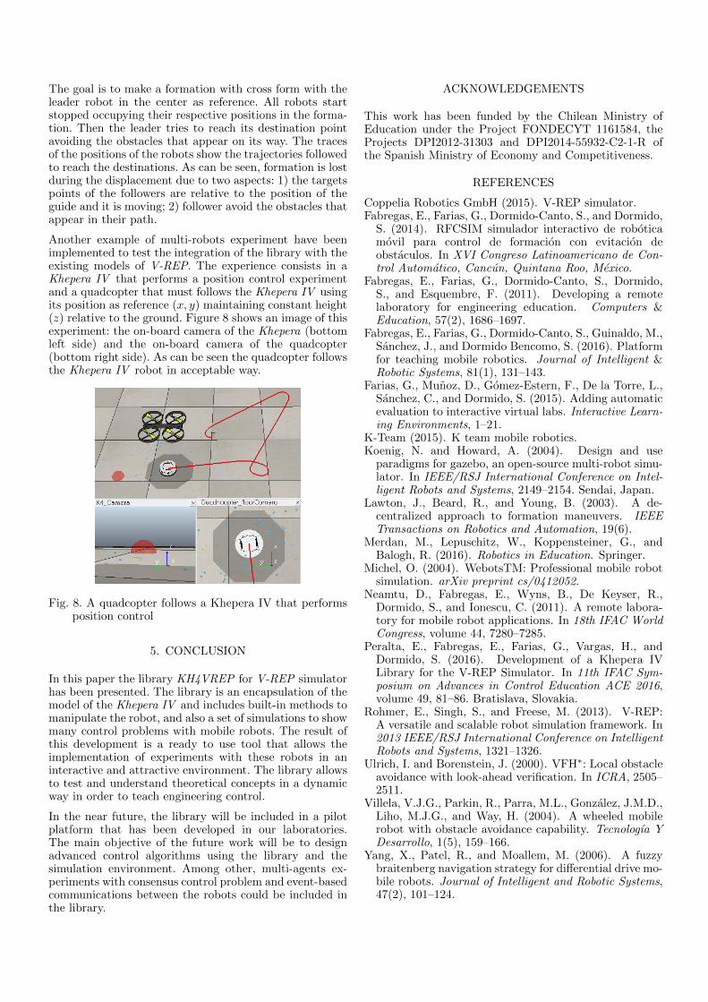
Another example of multi-robots experiment have beenimplemented to test the integration of the library with theexisting models of V-REP. The experience consists in aKhepera IV that performs a position control experimentand a quadcopter that must follows the Khepera IV usingits position as reference (x, y) maintaining constant height(z) relative to the ground. Figure 8 shows an image of thisexperiment: the on-board camera of the Khepera (bottomleft side) and the on-board camera of the quadcopter(bottom right side). As can be seen the quadcopter followsthe Khepera IV robot in acceptable way.

Fig. 8. A quadcopter follows a Khepera IV that performsposition control

5. CONCLUSION

In this paper the library KH4VREP for V-REP simulatorhas been presented. The library is an encapsulation of themodel of the Khepera IV and includes built-in methods tomanipulate the robot, and also a set of simulations to showmany control problems with mobile robots. The result ofthis development is a ready to use tool that allows theimplementation of experiments with these robots in aninteractive and attractive environment. The library allowsto test and understand theoretical concepts in a dynamicway in order to teach engineering control.

In the near future, the library will be included in a pilotplatform that has been developed in our laboratories.The main objective of the future work will be to designadvanced control algorithms using the library and thesimulation environment. Among other, multi-agents ex-periments with consensus control problem and event-basedcommunications between the robots could be included inthe library.

ACKNOWLEDGEMENTS

This work has been funded by the Chilean Ministry ofEducation under the Project FONDECYT 1161584, theProjects DPI2012-31303 and DPI2014-55932-C2-1-R ofthe Spanish Ministry of Economy and Competitiveness.

REFERENCES

Coppelia Robotics GmbH (2015). V-REP simulator.Fabregas, E., Farias, G., Dormido-Canto, S., and Dormido,

S. (2014). RFCSIM simulador interactivo de roboticamovil para control de formacion con evitacion deobstaculos. In XVI Congreso Latinoamericano de Con-trol Automatico, Cancun, Quintana Roo, Mexico.

Fabregas, E., Farias, G., Dormido-Canto, S., Dormido,S., and Esquembre, F. (2011). Developing a remotelaboratory for engineering education. Computers &Education, 57(2), 1686–1697.

Fabregas, E., Farias, G., Dormido-Canto, S., Guinaldo, M.,Sanchez, J., and Dormido Bencomo, S. (2016). Platformfor teaching mobile robotics. Journal of Intelligent &Robotic Systems, 81(1), 131–143.

Farias, G., Munoz, D., Gomez-Estern, F., De la Torre, L.,Sanchez, C., and Dormido, S. (2015). Adding automaticevaluation to interactive virtual labs. Interactive Learn-ing Environments, 1–21.

K-Team (2015). K team mobile robotics.Koenig, N. and Howard, A. (2004). Design and use

paradigms for gazebo, an open-source multi-robot simu-lator. In IEEE/RSJ International Conference on Intel-ligent Robots and Systems, 2149–2154. Sendai, Japan.

Lawton, J., Beard, R., and Young, B. (2003). A de-centralized approach to formation maneuvers. IEEETransactions on Robotics and Automation, 19(6).

Merdan, M., Lepuschitz, W., Koppensteiner, G., andBalogh, R. (2016). Robotics in Education. Springer.

Michel, O. (2004). WebotsTM: Professional mobile robotsimulation. arXiv preprint cs/0412052.

Neamtu, D., Fabregas, E., Wyns, B., De Keyser, R.,Dormido, S., and Ionescu, C. (2011). A remote labora-tory for mobile robot applications. In 18th IFAC WorldCongress, volume 44, 7280–7285.

Peralta, E., Fabregas, E., Farias, G., Vargas, H., andDormido, S. (2016). Development of a Khepera IVLibrary for the V-REP Simulator. In 11th IFAC Sym-posium on Advances in Control Education ACE 2016,volume 49, 81–86. Bratislava, Slovakia.

Rohmer, E., Singh, S., and Freese, M. (2013). V-REP:A versatile and scalable robot simulation framework. In2013 IEEE/RSJ International Conference on IntelligentRobots and Systems, 1321–1326.

Ulrich, I. and Borenstein, J. (2000). VFH∗: Local obstacleavoidance with look-ahead verification. In ICRA, 2505–2511.

Villela, V.J.G., Parkin, R., Parra, M.L., Gonzalez, J.M.D.,Liho, M.J.G., and Way, H. (2004). A wheeled mobilerobot with obstacle avoidance capability. Tecnologıa YDesarrollo, 1(5), 159–166.

Yang, X., Patel, R., and Moallem, M. (2006). A fuzzybraitenberg navigation strategy for differential drive mo-bile robots. Journal of Intelligent and Robotic Systems,47(2), 101–124.