A Key Predistribution Scheme forSensor Networks Using Deployment Knowledge

Wenliang Du, Jing Deng, Yunghsiang S. Han, and Pramod K. Varshney

W. Du, J. Deng, Y. S. Han, and P. K. Varshney, "A Key Pre-distribution Scheme for Sensor Networks Using

Deployment Knowledge," IEEE Transactions on Dependable and Secure Computing, vol. 3, no. 1, pp. 62-

77, January-March 2006. DOI: 10.1109/TDSC.2006.2

Made available courtesy of Institute of Electrical and Electronics Engineers: http://www.ieee.org/

*** (c) 2006 IEEE. Personal use of this material is permitted. Permission from IEEE must be obtained for

all other users, including reprinting/ republishing this material for advertising or promotional purposes,

creating new collective works for resale or redistribution to servers or lists, or reuse of any copyrighted

components of this work in other works.

Abstract:

To achieve security in wireless sensor networks, it is important to be able to encrypt messages sent among sensor

nodes. Keys for encryption purposes must be agreed upon by communicating nodes. Due to resource constraints,

achieving such key agreement in wireless sensor networks is nontrivial. Many key agreement schemes used in

general networks, such as Diffie-Hellman and public-key-based schemes, are not suitable for wireless sensor

networks. Predistribution of secret keys for all pairs of nodes is not viable due to the large amount of memory used

when the network size is large. Recently, a random key predistribution scheme and its improvements have been

proposed. A common assumption made by these random key predistribution schemes is that no deployment

knowledge is available. Noticing that, in many practical scenarios, certain deployment knowledge may be available

a priori, we propose a novel random key predistribution scheme that exploits deployment knowledge and avoids

unnecessary key assignments. We show that the performance (including connectivity, memory usage, and network

resilience against node capture) of sensor networks can be substantially improved with the use of our proposed

scheme. The scheme and its detailed performance evaluation are presented in this paper.

Index Terms: Wireless sensor networks, network security, key predistribution.

Article:

1 INTRODUCTION

RECENT advances in electronic and computer technologies have paved the way for the proliferation of wireless

sensor networks (WSN). Sensor networks usually consist of a large number of ultra-small autonomous devices.

Each device, called a sensor node, is battery powered and equipped with integrated sensors, data processing, and

short-range radio communication capabilities. In typical application scenarios, sensor nodes are spread randomly

over the deployment region under scrutiny and collect sensor data.

Sensor networks are being deployed for a wide variety of applications, including military sensing and tracking,

environment monitoring, patient monitoring and tracking, smart environments, etc. When sensor networks are

deployed in a hostile environment, security becomes extremely important as they are prone to different types of

malicious attacks. For example, an adversary can easily listen to the traffic, impersonate one of the network nodes

(in this paper, we use the terms sensors, sensor nodes, and nodes interchangeably), or intentionally provide

misleading information to other nodes. To provide security, communication should be encrypted and authenticated.

An open research problem is how to bootstrap secure communications among sensor nodes, i.e., how to set up

secret keys among communicating nodes?

This key agreement problem is a part of the key management problem, which has been widely studied in general

network environments. There are three types of general key agreement schemes: the trusted-server scheme, the

self-enforcing scheme, and the key predistribution scheme. The trusted-server scheme depends on a trusted server

for key agreement between nodes, e.g., Kerberos [1]. This type of scheme is not suitable for sensor networks

because there is usually no trusted infrastructure in sensor networks. The self-enforcing scheme depends on

asymmetric cryptography, such as key agreement using public key certificates. However, limited computation and

energy resources of sensor nodes often make it undesirable to use public key algorithms [2]. The third type of key

agreement scheme is key predistribution, where key information is distributed among all sensor nodes prior to

deployment. If we know which nodes are more likely to be in the same neighborhood before deployment, keys can

be decided a priori. However, because of the randomness of deployment, it might be infeasible to learn the set of

neighbors a priori.

There exist a number of key predistribution schemes. A naive solution is to let all the nodes carry a master secret

key. Any pair of nodes can use this global master secret key to achieve key agreement and obtain a new pairwise

key. This scheme does not exhibit desirable network resilience: If one node is compromised, the security of the

entire sensor network will be compromised. Some existing studies suggest storing the master key in tamper-

resistant hardware to reduce the risk, but this increases the cost and energy consumption of each sensor.

Furthermore, tamper- resistant hardware might not always be safe [3]. Another key predistribution scheme is to let

each sensor carry N – 1 secret pairwise keys, each of which is known only to this sensor and one of the other N – 1

sensors (assuming N is the total number of sensors). The resilience of this scheme is perfect because compromising

one node does not affect the security of communications among other nodes; however, this scheme is impractical

for sensors with an extremely limited amount of memory because N could be large. Moreover, adding new nodes

to a preexisting sensor network is difficult because the existing nodes do not have the new nodes‘ keys.

Eschenauer and Gligor proposed a random key predistribution scheme: Before deployment, each sensor node

receives a random subset of keys from a large key pool. To agree on a key for communication, two nodes find one

common key within their subsets and use this key as their shared secret key [4]. An overview of this scheme is

given in Section 3. The Eschenauer-Gligor scheme has further been improved by Chan et al. [5], by Du et al. [6],

and by Liu and Ning [7].

1.1 Outline of Our Scheme

Although the proposed schemes [4], [5], [6], [7] provided viable solutions to the key predistribution problem, they

have not exploited an important piece of information that might significantly improve their performance. This

piece of information is node deployment knowledge, which, in practice, can be derived from the way that nodes are

deployed.

Let us look at a deployment method that uses an airplane to deploy sensor nodes. The sensors are first prearranged

in a sequence of smaller groups. These groups are dropped out of the airplane sequentially as the plane flies

forward. This is analogous to parachuting troops or dropping cargo in a sequence. The sensor groups that are

dropped next to each other have a better chance of being close to each other on the ground. This spatial relation

between sensors derived prior to deployment can be useful for key predistribution. The goal of this paper is to

show that knowledge regarding the actual nonuniform sensor deployment can help to improve the performance of

key predistribution.

Knowing which sensors are close to each other is important for key predistribution. In sensor networks, long

distance peer-to-peer secure communication between sensor nodes is rare and unnecessary in many applications.

The primary goal of secure communication in wireless sensor networks is to provide such communications among

neighboring nodes. Therefore, the most important knowledge that can benefit a key-predistribution scheme is the

knowledge about the nodes that are likely to be the neighbors of each sensor node. If we know perfectly the

neighbors of each node in the network, key predistribution becomes trivial: For each node ni, we just need to

generate a pairwise key between ni and each of its neighboring nodes, and save these keys in ni‘s memory. This

guarantees that each node can establish a secure channel with each of its neighbors after deployment.

However, because of the randomness of deployment, it is unrealistic to know the exact set of neighbors of each

node, but knowing the set of possible or likely neighbors for each node is much more realistic. Still, the number of

possible neighbors can be very large and it may not be feasible for a sensor to store one secret key for each

potential neighbor due to memory limitations. This problem can be solved using the random key predistribution

scheme [4], i.e., instead of guaranteeing that any two neighboring nodes can find a common secret key with

certainty, we only guarantee that any two neighboring nodes can find a common secret key with a certain

probability p. In this paper, we exploit deployment knowledge in the random key predistribution scheme [4] such

that the probability p can be increased while the other performance metrics (such as security and memory usage)

are not degraded.

Deployment knowledge can be modeled using probability density functions (pdfs). When the pdf is uniform, no

information can be gained on where a node is more likely to reside. In this paper, we look at nonuniform pdfs,

which imply that we know that a sensor is more likely to be deployed in certain areas. We will show how this

knowledge can help to improve the random key predistribution scheme proposed by Eschenauer and Gligor [4] and

the scheme proposed by Du et al. [6]. To demonstrate the effectiveness of our method, we have studied a specific

distribution, the Normal (Gaussian) distribution, in great depth. Our results show substantial improvement over

existing schemes that do not exploit deployment knowledge.

1.2 Main Contributions of Our Scheme

The main contributions of this paper are summarized as follows:

1. We model node deployment knowledge in a wireless sensor network and develop a key predistribution

scheme based on this model. We are the first to attempt the use of deployment knowledge in key

predistribution.

2. We show that key predistribution with deployment knowledge can substantially improve a network‘s

connectivity (in terms of secure links) and resilience against node capture and reduce the amount of

memory required.

2 RELATED WORK

The Eschenauer-Gligor scheme [4] has been briefly described earlier in Section 1. We will give a more detailed

description of this scheme in Section 3. Based on the Eschenauer-Gligor scheme, Chan et al. proposed a q-

composite random key predistribution scheme [5]. The major difference between this scheme and the Eschenauer-

Gligor scheme is that q common keys (q ≥ 1), instead of just a single one, are needed to establish secure

communications between a pair of nodes. It is shown that, by increasing the value of q, network resilience against

node capture is improved, i.e., an attacker has to compromise many more nodes to achieve a high probability of

compromised communication.

Du et al. proposed a new key predistribution scheme [6], which substantially improved the resilience of the

network compared to the existing schemes. This scheme exhibits a nice threshold property: When the number of

compromised nodes is less than the threshold, the probability that nodes other than the compromised ones are

affected is close to zero. This desirable property lowers the initial payoff of small-scale network breaches to an

adversary and makes it necessary for the adversary to attack a significant portion of the network. A similar method

was also developed by Liu and Ning [7].

Liu and Ning independently developed a scheme using predeployment knowledge [8] when a preliminary version

of this paper [9] was prepared. However, this paper and its preliminary version introduce a novel group-based

deployment model. This group-based deployment model is further explored by Huang et al. [10].

Perrig et al. proposed SPINS, a security architecture specifically designed for sensor networks [2]. In SPINS, each

sensor node shares a secret key with the base station. Two sensor nodes cannot directly establish a secret key.

However, they can use the base station as a trusted third party to set up the secret key. Chan and Perrig proposed

PIKE, a class of key-establishment protocols that involves using one or more sensor nodes as a trusted

intermediary to facilitate key establishment [11]. Anderson et al. also studied how the key distribution problem can

be dealt with in environments with a partially present, passive adversary [12]. Zhu and Setia [13] proposed a key

management scheme based on the assumption that there exists a lower bound on the time interval that is necessary

for an adversary to compromise a sensor.

Blundo et al. proposed several schemes which allow any group of t parties to compute a common key while being

secure against collusion between some of them [14]. These schemes focus on saving communication costs while

memory constraints are not placed on group members.

Several other key distribution schemes have been proposed for mobile computing, although they are not

specifically targeted at sensor networks. Tatebayashi et al. considered key distribution for resource-starved devices

in a mobile environment [15]. Other key agreement and authentication protocols include the one by Beller and

Yacobi [16]. A survey on key distribution and authentication for resource-starved devices in mobile environments

is given by Boyd and Mathuria [17]. The majority of these approaches rely on asymmetric cryptography, which is

not a feasible solution for sensor networks [2].

3 BACKGROUND

3.1 The Eschenauer-Gligor (EG) Scheme

The Eschenauer-Gligor scheme (referred to as the basic scheme or the EG scheme hereafter) proposed by

Eschenauer and Gligor [4] consists of three phases: key predistribution, shared-key discovery, and path-key

establishment.

In the key predistribution phase, each sensor node randomly selects τ distinct cryptographic keys from a key pool S

and stores them in its memory. This set of τ keys is called the node‘s key ring. The number of keys in the key pool,

ISI, is chosen such that two random subsets of size τ in S share at least one key with some probability p.

After the nodes are deployed, a key-setup phase is performed. During this phase, each pair of neighboring nodes

attempt to find a common key that they share. If such a key exists, the key is used to secure the communication

link between these two nodes. After key-setup is complete, a graph (called key graph) of secure links is formed.

Nodes can then set up path keys with their neighbors with whom they do not share keys. If the key graph is

connected, a path can always be found from a source node to any of its neighbors. The source node can then

generate a path key and send it securely via the path to the target node.

The size of the key pool S is critical to both the connectivity and the resilience of the scheme. Connectivity is

defined as the probability that any two neighboring nodes share one key. Resilience is defined as the fraction of the

secure links that are compromised after a certain number of nodes are captured by the adversaries.

At one extreme, if the size of S is one, i.e., |S| = 1, the scheme is actually reduced to the naive master-key scheme.

This scheme yields a high connectivity, but it is not resilient against node capture because the capture of one node

can compromise the whole network. At the other extreme, if the key pool is very large, e.g., |S| = 100,000,

resilience becomes much better, but connectivity of the sensor network becomes low. For example, as indicated by

Eschenauer and Gligor [4], in this case, even when each sensor selects τ = 200 keys from this large key pool S, the

probability that any two neighboring nodes share at least one key is only 0.33.

How can we use a large key pool while still maintaining high connectivity and the same memory usage? In this

paper, we use deployment knowledge to solve this problem.

3.2 The Du-Deng-Han-Varshney (DDHV) Scheme

Blom proposed a key predistribution method that allows any pair of nodes in a network to be able to derive a

pairwise secret key [18]. It has the property that, as long as no more than λ nodes are compromised, all

communication links of noncompromised nodes remain secure (we refer to this as being ―λ-secure‖). We now

briefly describe Blom‘s scheme (we have made some slight modifications to the scheme in order to make it more

suitable for sensor networks, but the essential features remain unchanged).

We assume some agreed-upon (λ + 1) × N matrix G over a finite field GF(q), where N is the size of the network

and q > N. This matrix G is public information and may be shared by different systems; even adversaries are

allowed to know G. During the key generation phase, the base station creates a random (λ + 1) × (λ + 1) symmetric

matrix D over GF(q), and computes an N × (λ + 1) matrix A = (D • G)T, where (D • G)

T is the transpose of D • G.

Matrix D must be kept secret, and should not be disclosed to adversaries or to any sensor nodes (although, as will

be discussed, one row of (D • G)T will be disclosed to each sensor node). Because D is symmetric, it is easy to see

that

i.e., A • G is a symmetric matrix. If we let K = A • G, we know that Kij = Kji, where Kij is the element in the ith

row and jth column of K. The idea is to use Kij (or Kji) as the pairwise key between node i and node j. Fig. 1

illustrates how the pairwise key Kij = Kji is generated. To carry out the above computation, nodes i and j should be

able to compute Kij and Kji, respectively. This can be easily achieved using the following key predistribution

scheme, for k = 1;...; N:

1. store the kth row of matrix A at node k, and

2. store the kth column of matrix G at node k.1

Then, when nodes i and j need to establish their pairwise key, they first exchange their columns of G and then

compute Kij and Kji, respectively, using their private rows of A. Because G is public information, its columns can

be transmitted in plaintext. It has been shown [18] that the above scheme is λ-secure if any λ + 1 columns of G are

linearly independent. This λ-secure property guarantees that no coalition of up to λ nodes (not including i and j)

have any information about Kij or Kji.

We define the set of keys generated from A and G as a key space. According to the Blom scheme, if any two nodes

carry their corresponding information from the same key space, they can find a common key between themselves.

Roughly speaking, Blom‘s scheme uses a single key space. By changing the values of matrices D and G, we can

create different key spaces.

Motivated by the random key predistribution schemes [4], [5], Du et al. developed an improved key predistribution

scheme using multiple key spaces (we call it the DDHV scheme) [6]. The DDHV scheme first constructs ! spaces

using Blom‘s scheme and then has each sensor node carry key information from τ (with 2 < τ < ω) randomly

selected key spaces. Now (from the properties of the underlying Blom scheme), if two nodes carry key information

from a common space they can compute a shared key. Of course, unlike Blom‘s scheme, it is no longer certain that

two nodes can generate a pairwise key; instead (as in the Eschenauer-Gligor random key predistribution scheme),

such a connectivity is probabilistic.

It should be noted that, when a key space has λ = 0, a compromise of one (i.e., λ + 1) node from this key space will

compromise the entire key space. This is equivalent to having one key in this key space. Therefore, by letting λ =

1 In practice, sensors need not store the whole column because each column can be generated from a single field element [6].

0, each key space collapses to one key and, thus, the DDHV scheme reduces to the EG scheme. From this

perspective, the EG scheme is actually a special case of the DDHV scheme. Therefore, in this paper, we focus only

on the DDHV scheme.

4 MODELING OF THE DEPLOYMENT KNOWLEDGE

We assume that sensor nodes are static once they are deployed. We define deployment point as the desired point

where a sensor is to be deployed. This is not likely the location where the sensor resides eventually. The sensor

node can reside at points around this desired point according to a certain pdf. As an example, let us consider the

case where sensors are deployed by being dropped from a helicopter. The deployment point is the location of the

helicopter. We also define resident point for a sensor as the point where the sensor finally resides.

4.1 Group-Based Deployment Model

In practice, it is quite common that nodes are deployed in groups, i.e., a group of sensors are deployed at a single

deployment point, and the pdfs of the final resident points of all the sensors in each batch (or group) are the same.

In this work, we assume such a group-based deployment and we model the deployment knowledge as follows (we

call this model the group-based deployment model):

1. N sensor nodes to be deployed are divided into t × n equal size groups so that each group, Gi,j, for i = 1,...,t

and j = 1,..., n, is deployed from the deployment point with index (i,j). Let (xi, yj) represent the deployment

point for group Gi,j.

2. The deployment points are arranged in a grid. Note that the scheme we develop for grid-based deployment

can be easily extended to different deployment strategies. We choose this specific strategy because it is

quite common in realistic scenarios.

3. During deployment, the resident points of the node k in group Gi,j follow the pdf f(x,y|k ∈ Gi,j). An example

of the pdf is a two-dimensional Gaussian distribution.

When f(x,y|k ∈ Gi,j) is a uniform distribution over the deployment region for all Gi,js, we do not know which nodes

are more likely to be close to each other a priori because the resident point of a node can be anywhere within the

region with the same probability. However, when f(x,y|k ∈ Gi,j) is a nonuniform distribution, we can determine

which nodes are more likely to be close to each other. For example, with Gaussian distribution, we know that the

distance between a resident point and the deployment point is less than 3σ with probability 0.9987 (where u is the

standard deviation of the Gaussian distribution). If the deployment points of two groups are 6σ away, then the

probability of two nodes from these two different groups being located near each other is very low. Therefore, the

probability that two nodes from two different groups become neighbors decreases with an increase of the distance

between the two deployment points.

Recall that, in the Eschenauer-Gligor random key predistribution scheme [4] and the DDHV scheme [6], when the

size of the key-space pool S becomes smaller, connectivity increases. Since these schemes assume no deployment

knowledge (i.e., the distribution f(x,y|k ∈ Gi,j) is uniform), every node should choose from the same key-space pool

because they are equally likely to be neighbors. However, as we have discussed, when the function f(x,y|k ∈ Gi,j) is

nonuniform, we know that nodes from a specific group are more likely to be neighbors of nodes from the same

group and those from nearby groups. Therefore, when two groups are far away from each other, their key-space

pools should be different, rather than the same global key-space pool S.

We use Si,j to represent the key-space pool used by group Gi,j; the union of Si,j (for i = 1,..., t and j = 1,..., n) equals

S. We use |Sc| to represent the size of Si,j (for the sake of simplicity, we let all Si,js have the same size in this paper).

Based on a specific deployment distribution, we can develop a scheme such that, when the deployment points of

two groups and

are farther away from each other, the amount of overlap between and

becomes smaller or zero.

4.2 Deployment Distribution

There are many different ways to deploy sensor networks, for example, sensors could be deployed using an

airborne vehicle. The actual model for deployment distribution depends on the deployment method. Our key

predistribution scheme is for the most part model independent. We propose our scheme in a manner whereby it can

be instantiated to use other deployment models. To keep the presentation concrete, we use a specific model,

namely, we model the sensor deployment distribution as a two- dimensional Gaussian distribution (also called

Normal distribution). Our methodology should be easily adaptable to other deployment models. In practice, we

need to develop the deployment model based on the actual deployment method. How to develop the model is

beyond the scope of this paper.

We assume that the deployment distribution for any node k in group Gi,j follows a two-dimensional Gaussian

distribution. When the deployment point of group Gi,j is at (xi, yj), we have µ = (xi, yj) and the pdf for node k in

group Gi,j is the following [19]:

∈

Although the distribution function for each single group is nonuniform, we still prefer the sensor nodes to be

evenly deployed throughout the entire region. By choosing a proper distance between the neighboring deployment

points with respect to the value of σ in the pdf of each deployment group, the probability of finding a node in each

small region can be made approximately equal. Assuming that a sensor node is selected to be in a given group with

an equal probability,

, the average deployment distribution (pdf) of any sensor node over the entire region is:

∈

To see the overall distribution of sensor nodes over the entire deployment region, we have plotted foverall in (2) for 6

x 6 = 36 groups over a 600m × 600m square region with the deployment points 2σ = 100m apart (assuming σ = 50).

Fig. 2a shows all the deployment points and Fig. 2b shows the overall pdf. From Fig. 2b, we can see that the pdf is

almost flat (i.e., nodes are fairly evenly distributed) in the whole region except near the boundaries.

5 KEY PREDISTRIBUTION USING DEPLOYMENT KNOWLEDGE

Based on the deployment model described in the previous section, we propose a new random key predistribution

scheme, which takes advantage of deployment knowledge. This new scheme is based on the original DDHV

scheme, so we call it the DDHV-D scheme.2 In this scheme, we assume that the sensor nodes are evenly divided

into t × n groups Gi,j, for i = 1,..., t, and j = 1,..., n. We assume that the global key-space pool is S with size |S| and

also assume that the deployment points are arranged in a grid depicted in Fig. 2a. Each node carries T key spaces.

5.1 Key Predistribution Scheme

The goal of this scheme is to allow sensor nodes to find a common secret key with each of their neighbors after

deployment. Our scheme consists of three phases: key predistribution, shared-key discovery, and path-key estab-

lishment. The last two phases are exactly the same as the DDHV scheme [6], but, because of deployment

knowledge, the first phase is considerably different.

5.1.1 Step 1: Key Predistribution Phase

This phase is conducted offline and before the sensors are deployed. First, we need to divide the key-space pool S

into t x n key-space pools Si,j (for i = 1,..., t and j = 1,..., n), with Si,j corresponding to the deployment group Gi,j.

We say that two key-space pools are neighbors (or near each other) if their corresponding deployment groups are

deployed in neighboring (or nearby) locations. The goal of setting up the key-space pools Si,j is to allow the nearby

key-space pools to share more key spaces, while those far away from each other share fewer key spaces or no key

space at all. Steps for setting up key-space pools will be discussed in detail later.

After the key-space pools are set up, for each sensor node in the deployment group Gi,j, we randomly select T key

spaces from its corresponding key-space pool Si,j; then, for each selected key space, we load the corresponding row

of its matrix (i.e., matrix A) into the memory of the node.

5.1.2 Step 2: Shared-Key Discovery Phase

After deployment, each node needs to discover whether it shares any key space with its neighbors. To do this, each

node broadcasts a message containing the indices of the key spaces it carries. Each neighboring node can use these

broadcast messages to find out if there exists a common key space it shares with the broadcasting node. If such a

key space exists, using the Blom scheme, the two neighboring nodes can derive a pairwise key from the common

key space and use the key to secure the communication channel between themselves.

After the above step, the entire sensor network forms a Key-Space Sharing Graph GKS, which is defined in the

following:

Definition 1 (Key-Space Sharing Graph). Let V represent all the nodes in the sensor network. A Key-Space

Sharing Graph GKS(V; E) is constructed in the following manner: For any two nodes i and j in V, there exists an

2 ―D‖ after the hyphen indicates the use of deployment knowledge.

edge between them if and only if 1) nodes i and j have at least one common key space and 2) nodes i and j can

reach each other within the wireless transmission range, i.e., in a single hop.

5.1.3 Step 3: Path-Key Establishment Phase

It is possible that two neighboring nodes cannot find any common key space between them. In this case, they need

to find a secure way to agree upon a common key. We now show how two neighboring nodes, i and j, who do not

share a common key space could still come up with a secret key between them. The idea is to use the secure

channels that have already been established in the key-space sharing graph GKS: As long as the graph is

connected, two neighboring nodes i and j can always find a path in GKS from i to j. Assume that the path is i, v1,...,

vh, j. To find a common secret key between i and j, i first generates a random key K. Then, i sends the key to v1

using the secure link between i and v1, v1 forwards the key to v2 using the secure link between v1 and v2 and so on

until j receives the key from vh. Nodes i and j use this secret key K as their pairwise key. Because the key is always

forwarded over a secure link, no nodes beyond this path can find out the key.

To find such a secure path for nodes i and j, the easiest way is to use flooding [20], a common technique used in

multihop wireless networks. As we will show later in our analysis, in practice, the probability that the secure path

between i and j is within three hops is very high (close to one). Therefore, we can always limit the lifetime of the

flooding message to three hops to reduce flooding overhead.

5.2 Setting Up Key-Space Pools

Next, we show how to assign key spaces to each key-space pool Si,j, for i = 1,..., t and j = 1,..., n, such that key-

space pools corresponding to nearby deployment points have a certain number of common key spaces. In our

scheme, we have:

1. Two horizontally or vertically neighboring key- space pools share exactly a|Sc| key spaces,3 where 0 < a <

0.25.

2. Two diagonally neighboring key-space pools share exactly b|Sc| key spaces, where 0 < b < 0.25 and 4a + 4b

= 1.

3. Two nonneighboring key-space pools share no key spaces.

We call a and b the overlapping factors. To achieve the above properties, we divide the key spaces in each key-

space pool into eight partitions (see Fig. 3a). Key spaces in each partition are those key spaces that are shared

between the corresponding neighboring key-space pools. For example, in Fig. 3a, the partition in the upper left

corner of E consists of b • |Sc| key spaces shared between A and E; the partition in the left part of E consists of a •

|Sc| key spaces shared between D and E.

Given the global key-space pool S and the overlapping factor a and b, we now describe how we can select key

spaces for each key-space pool Si,j for i = 1,..., t and j = 1, ... , n. The procedure is also depicted in Fig. 3b for a 4 x

4 case. First, key spaces for the first group S1,1 are selected from S; then, key spaces for the groups in the first row

are selected from S and their left neighbors. Then, key spaces for the groups in the second row to the last row are

selected from S and their left, upper-left, upper, and upper- right neighbors. For each row, we conduct the process

from left to right. The following procedure describes how we choose key spaces for each key-space pool:

1. For group S1,1, select |Sc| key spaces from the global key-space pool S; then, remove these |Sc| key spaces

from S.

2. For group Si,j, for j = 2,..., n, select a • |Sc| key spaces from the key-space pool S1,j-1; then, select w = (1 – a).

|Sc| key spaces from the global key-space pool S and remove the selected w key spaces from S.

3. For group Si,j, for i = 2,..., t and j = 1,..., n, select a • |Sc| key spaces from each of the key-space pools Si–1,j

and Si,j–1 if they exist; select b • |Sc| key spaces from each of the key-space pools Si–1,j–1 and Si–1,j+1 if they

3 If a|Sc| is not an integer, should be used instead.

exist; then, select w (defined below) key spaces from the global key-space pool S and remove these w key

spaces from S.

Note that, after any group (e.g., G1) selects s key spaces (s = a • |Sc| or s = b • |Sc|) from its neighbor (e.g., G2), no

other neighboring groups of G1 or G2 can select any one of these s key spaces, i.e., these s key spaces are only

shared by G1 and G2. In other words, no key space is shared by more than two neighboring groups in our scheme.

Although this requirement is not necessary in practice, it significantly simplifies our analysis.

6 PERFORMANCE AND SECURITY: ANALYTICAL RESULTS

In this section, we analyze the performance and security of our scheme. We present our analytical results on the

following two metrics:

Local connectivity. We use local connectivity to refer to the probability of any two neighboring nodes

sharing at least one key space. We use plocal and p interchangeably to refer to the local connectivity. The

local connectivity directly affects the performance of the scheme.

Resilience against node capture. In a hostile environment, adversary can mount physical attacks on a sensor

node after it is deployed and read secret information from its memory. We need to find how a successful

attack on x sensor nodes by an adversary affects the rest of the network. In particular, we want to find the

fraction of additional communications (i.e., communications among uncaptured nodes) that an adversary

can compromise based on the information retrieved from the x captured nodes. In this analysis, we did not

measure the impact of the compromise of the path keys.

6.1 Computing Local Connectivity

We randomly pick any two nodes u and v in the network. Let A(u; v) be the event that u and v are neighbors; let

B(u; v) be the event that u and v share at least one common key space. Therefore, the local connectivity plocal (i.e.,

the probability of two neighboring nodes being able to find a common key space) is the following conditional

probability:

Since u and v are picked randomly, the above probability is the average over all possible pairs of nodes. Defining

ψ as the set of all deployment groups in our scheme, we have

∈ ∈

∈ ∈

∈ ∈

∈ ∈

∈ ∈

Note that, in the above equation, because the two nodes u and v are selected independently and each of them is

selected to be in any given deployment group with an equal probability, we have Pr(u ∈ Gi and v ∈ Gj) =

,where n • t is the number of deployment groups. Similar to the above equation for Pr(A(u,v)), we have the

following equation:

∈ ∈

∈ ∈

∈ ∈

∈ ∈

∈ ∈

Because events B(u,v|u ∈ Gi and v ∈ Gj) and A(u,v|u ∈ Gi and v ∈ Gj) are independent,4 we have the following:

∈ ∈

∈ ∈

∈ ∈

Therefore, to compute the local connectivity, we just need to compute Pr(A(u, v) | u ∈ Gi and v ∈ Gj) and Pr(B(u, v)

| u ∈ Gi and v ∈ Gj). To simplify notations, we use ni to replace u and nj to replace v; the subscripts i and j indicate

that ni is from Gi and nj is from Gj. We can, therefore, omit the condition (u ∈ Gi and v ∈ Gj) in our notation. The

probability of local connectivity in (3) becomes

∈ ∈

∈ ∈

Therefore, we need to compute Pr(A(ni, nj)) and Pr(B(ni, nj)) in order to find plocal. It should be noted that Pr(A(ni,

nj)) solely depends on the deployment model, while Pr(B(ni, nj)) solely depends on the key predistribution.

6.1.1 Computing Pr(A(ni, nj))

We present our calculation of Pr(A(ni, nj)), the probability that two sensors deployed from groups Gi and Gj are

physical neighbors.

We divide the entire deployment region into many infinitesimal rectangular areas of size dx dy. Let B = (x,y)

represent a point in the region, and we use θ(dx, dy) to represent the infinitesimal rectangular area around B.

4 Note that unconditional events B(u, v) and A(u, v) are not independent because they both depend on the deployment groups that u and v

come from.

Assuming that the x-axis of the deployment region ranges from 0 to X and the y-axis ranges from 0 to Y, we can

use the following formula to compute the probability that ni and nj are neighbors:

The probability that the node nj (from group Gj) resides within this small rectangle area θ(dx; dy) can be computed

directly using the probability density function fR of the deployment:

∈

where is the distance between θ and the deployment point of group j. Based on the two-dimensional Gaussian

deployment distribution as shown in (1), we have

∈

Next, we show how Pr(A(ni, nj) | nj is in θ(dx, dy)) can be computed. We use z to represent the distance from point

θ to the deployment point of group Gi. We draw two circles. The first circle has a radius ℓ and is centered at i, the

deployment point of group Gi. We call this circle the i-circle. The second circle has a radius R (where R is the

wireless transmission range) and is centered at θ = (x, y). We call this circle the θ-circle. When two circles

intersect, we call the i-circle‘s arc within the θ-circle the Larc and we use Larc(ℓ, z, R) to represent the length of the

arc. We now consider an infinitesimal ring area Larc(ℓ, z, R). dℓ. The bold areas in Fig. 4a and Fig. 4b show the

infinitesimal ring areas. Using geometry, we can compute the length of the arc using the following formula:

ℓ ℓ ℓ

ℓ

Recall that fR(ℓ | ni ∈ Gi) represents the probability density function of the deployment for group Gi. Therefore, the

probability that the node ni resides within this small ring area is

ℓ ∈ ℓ ℓ

We define g(z | ni ∈ Gi) as the probability that the sensor node ni from group Gi resides within the θ-circle, where z

is the distance between θ and the deployment point of group Gi. It is not hard to see that

∈

To calculate g(z | ni ∈ Gi), we integrate the probabilities over all the ring areas (for different ℓ) within the 0-circle.

Therefore, when z > R (as shown in Fig. 4a),

∈ ℓ ∈ ℓ ℓ

When z < R (as shown in Fig. 4b),

∈ ℓ ℓ ∈ ℓ

ℓ ∈ ℓ ℓ

Combining the above equations together, we get

∈

∈

where (respectively, is the distance between the deployment point of Gi (respectively, Gj) and θ = (x, y).

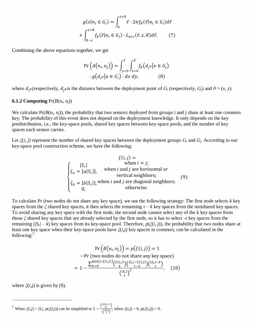
6.1.2 Computing Pr(B(ni, nj))

We calculate Pr(B(ni, nj)), the probability that two sensors deployed from groups i and j share at least one common

key. The probability of this event does not depend on the deployment knowledge. It only depends on the key

predistribution, i.e., the key-space pools, shared key spaces between key-space pools, and the number of key

spaces each sensor carries. Let ξ(i, j) represent the number of shared key spaces between the deployment groups Gi and Gj. According to our

key-space pool construction scheme, we have the following:

To calculate Pr (two nodes do not share any key space), we use the following strategy: The first node selects k key

spaces from the ξ shared key spaces, it then selects the remaining τ – k key spaces from the nonshared key spaces.

To avoid sharing any key space with the first node, the second node cannot select any of the k key spaces from

those ξ shared key spaces that are already selected by the first node, so it has to select -r key spaces from the

remaining (|Sc| – k) key spaces from its key-space pool. Therefore, p(ξ(i, j)), the probability that two nodes share at

least one key space when their key-space pools have ξ(i,j) key spaces in common, can be calculated in the

following:5

where ξ(i,j) is given by (9).

5 When ξ(i,j) = |Sc|, p(ξ(i,j)) can be simplified to

; when ξ(i,j) = 0, p(ξ(i,j)) = 0.

6.2 Resilience Analysis

In order to analyze the resilience of the DDHV-D scheme, we need to have a model for the adversary‘s attacks.

While establishing such models, we consider a realistic scenario in which the adversary intrudes a region inside the

sensor network and randomly captures and compromises xc sensors within this region. We explain the attack model

in the following:

We assume that the adversary captures nodes randomly within a region.

The region is assumed to be a circle6 centered at point with coordinate (x,y) with radius Rc. We term such a

circle the attack circle and call Rc the attack radius. An example of an attack circle is shown in Fig. 5. Note

that, when the circle is large enough to contain the entire deployment region, the attack model reduces to

the uniform-random attack, in which the probability that any node in the entire deployment region is

compromised is the same.

Under this attack model, we analyze the resilience of our key predistribution scheme. We explore the effect of the

capture of xc sensor nodes by an adversary on the security of the rest of the network. In particular, we calculate an

upper bound on the fraction of additional communication (i.e., communication among the uncaptured nodes) that

an adversary can compromise based on the information retrieved from the xc captured nodes. To compute this

fraction, we first compute the probability that any one of the additional communication links is compromised after

xc nodes are captured. Note that we only consider the links in the key-space-sharing graph and each of these links

is secured using a key computed from the common key space shared by the two nodes of this link.

We summarize our approach for resilience analysis in the following; the detailed derivation is presented in

Appendix A. Based on the above assumptions, we can calculate, among all sensors in the attack circle, the average

number of sensors that are deployed from each specific group. Since the adversary compromises xc sensors ran-

domly inside the circle, the average number of compromised sensors that are deployed from the specific group can

be derived. Based on the key-space pool sharing technique shown in Fig. 3b, we derive the average number of

sensors that are compromised and are carrying key information from the same key-space pool. Then, we use the

method by Du et al. [6] to calculate an upper bound on the fraction of additional communication that an adversary

can compromise based on the information retrieved from the xc captured nodes.

6 The analysis of other shapes is similar, albeit with more complicated formulas.

The main result, Inequality (12) in Appendix A, gives the upper bound on the fraction of additional communication

that an adversary can compromise based on the information retrieved from the xc captured nodes.

7 PERFORMANCE AND SECURITY EVALUATION: NUMERICAL RESULTS

An important goal of this study is to understand the performance of the DDHV-D scheme. However, because of

the complexity of the analytical results obtained for local connectivity and resilience, it is difficult to understand

the performance from the equations that we have derived. In this section, we present numerical results

corresponding to those derived equations. We show the performance of the DDHV-D scheme as well as the

comparisons with the existing key predistribution schemes. More importantly, we will use the numerical results to

understand the relationships among the parameters λ, memory usage m, local connectivity plocal, and resilience, as

their relationships are difficult to understand from the rather complicated analytical results. Note that m is defined

in units of key size; namely, if each key is 64 bits long, then the total amount of memory usage is 64 • m bits. The

relationship between the memory usage m and the number (τ) of key spaces each sensor can carry is the following

[6]:

7.1 System Configuration

In our numerical analysis and simulations, we use the following setup:

The number of sensor nodes in the sensor network is 10,000.

The deployment area is 1000m x 1000m.

The area is divided into a grid of size

100 = t × n = 10 × 10,

with each grid cell of size 100m × 100m.

The center of each grid cell is the deployment point (see Fig. 2a).

The wireless communication range for each node is R = 40m.

We assume that the node deployment follows a two- dimensional Gaussian distribution.

7.2 Connectivity

We show the results for both local connectivity and global connectivity. Global connectivity refers to the ratio of

the number of nodes in the largest isolated component in the final key-space-sharing graph to the size of the whole

network. If the ratio equals 99 percent, it means that 99 percent of the sensor nodes are connected and the

remaining 1 percent are unreachable from the largest isolated component. So, the global connectivity metric

indicates the percentage of nodes that are wasted because of their unreachability. Both global connectivity and

local connectivity are affected by the key predistribution scheme.

7.2.1 Local Connectivity

In this experiment, we evaluate how much the deployment knowledge can improve the local connectivity. We

conduct two evaluations, one for the EG scheme (i.e., λ = 0), and the other for the DDHV scheme (we set λ = 19).

A number of parameters can affect the local connectivity; to simplify the evaluation, we set a = 0.15 and b = 0.10.

In addition, we make the local connectivity for m = 100 the same for both EG and DDHV schemes. Once these

parameters are fixed, we can decide the size of the global key-space pool and the local key-space pools. Then,

based on (4), we can compute plocal for the EG, EG-D,7 DDHV, and DDHV-D schemes for various memory usage

scenarios. The results are plotted in Fig. 6. Fig. 6a and Fig. 6b clearly shows that the deployment-knowledge-based

EG-D and DDHV-D schemes significantly improve the local connectivity of their counterparts.

There are two ―abnormal‖ phenomena in Fig. 6b. First, it seems that plocal for DDHV-D can never reach 1. The

reason for this phenomenon is that some neighboring nodes might come from nonneighboring deployment groups.

According to our key predistribution scheme, they do not share any key space because their deployment groups are

not neighbors. Therefore, the local connectivity can never reach 1. The second abnormal phenomenon is the

appearance of discrete steps for both DDHV and DDHV-D schemes. This is because of rounding: When |S| is

fixed, the only parameter that can affect the local connectivity is τ, the number of key spaces carried by each

sensor. Because

, there will be discrete steps for T when m is increased, causing the discrete

steps for plocal.

7.2.2 Global Connectivity

It is possible that the key-space-sharing graph in our scheme has a high local connectivity, but the graph can still

have isolated components. Since those components are disconnected, no secure links can be established among

them. Therefore, it is important to determine whether the graph will have too many isolated components. To this

end, we measure the global connectivity of the key-spacesharing graph, namely, we measure the ratio of the size of

the largest isolated component in G and the size of the whole network. We consider that all the nodes that are not

connected to the largest isolated component are useless nodes because they are ―unreachable‖ via secure links.8

When node distribution and key sharing are uniform, global connectivity can be estimated using the local

connectivity and other network parameters using Erdos and Re´nyi random graph theorem [21], just like what has

been done by Eschenauer and Gligor [4] and Chan et al. [5]. However, since neither our node distribution nor our

key sharing is uniform, Erdos and Re´nyi‘s random graph theorem is not a good estimation method. Recently,

Shakkottai et al. have determined the connectivity of a wireless sensor grid network with unreliable nodes [22].

Their results have been corrected and further improved by Kumar et al. [23]. In our future work, we will estimate

the global connectivity by using the results given by Kumar et al. [23]. In this work, we only use simulation to

estimate global connectivity. We use the configuration described in Section 7.1 to conduct the simulation. The

relationships between the local connectivity and the global connectivity are shown in Table 1.

7 EG-D stands for the scheme that combines the original EG scheme and deployment knowledge. It is a special case of DDHV-D (i.e., the

A = 0 case). 8 Some of the ―unreachable‖ nodes might be reachable physically because they are within the communication range, but they cannot find

a common key with any of the nodes in the largest isolated component.

The simulation results indicate that, when the local connectivity plocal reaches 0.697, only 0.12 percent of the

sensor nodes are wasted due to the lack of secure links; when plocal reaches 0.956, no nodes are wasted. These

results exclude those nodes that are not within the communication range of the largest isolated component because

they are caused by deployment, not by our key predistribution scheme.

7.3 Resilience against Node Capture

We assume that an adversary can mount a physical attack on a sensor node after it is deployed and read secret

information from its memory. We need to find how a successful attack on x sensor nodes by an adversary affects

the rest of the network. In particular, we want to find the fraction of additional communication (i.e.,

communications among uncaptured nodes) that an adversary can compromise based on the information retrieved

from the x captured nodes.

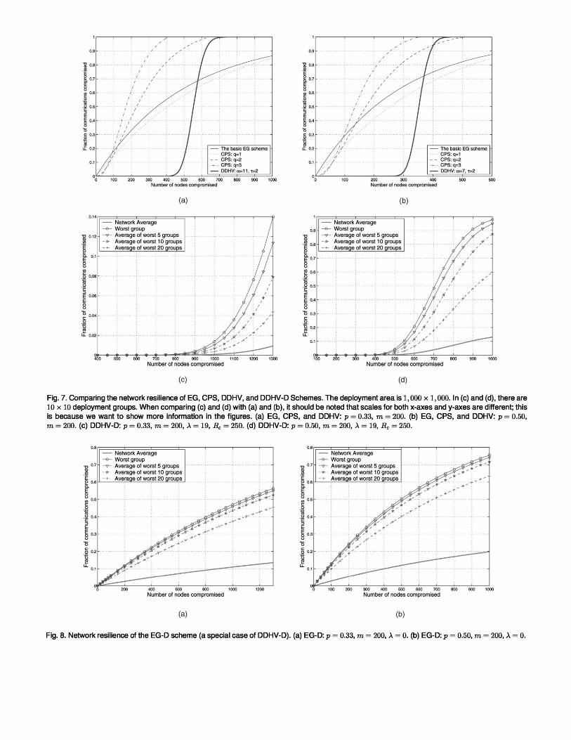
7.3.1 Comparison with the Existing Schemes

In Fig. 7, we show the numerical results on the resilience performance of the DDHV-D scheme against node

compromise (capture). The attack circle is assumed to be Rc = 250 m. Our main performance metric is, Pc, the

fraction of communication links that are compromised when x nodes are captured. We plot Pc for the Eschenauer-

Gligor scheme (EG) [4], the Chan-Perrig-Song (CPS) scheme [5], and the DDHV scheme [6] in Figs. 7a and 7b.

We plot Pc of the DDHV-D scheme in Figs. 7c and 7d. We use average to represent the average number of

communication links compromised in the network or in a set of groups.

In Figs. 7c and 7d, the network average curve shows the average of all groups in the network. Since the adversary

only captures nodes inside the attack circle, only the keys of a few groups are affected. Those groups that are far

away from this region are not likely to be affected at all. Therefore, the resilience performance of the network on

average is very good for the x values that we show. However, if we calculate the average resilience performance of

those groups that have been affected the most, the ―worst groups,‖ their resilience is quite different from the

network average. For example, if we consider the worst group, Pc approaches 1 more quickly than the others.

These are not surprising results considering that the adversary is concentrating its efforts in the same area as we are

measuring. As we increase the number k in the ―k worst groups‖ performance, Pc increases more slowly. Such a

trend is shown in both of Figs. 7c and 7d.

As we mentioned before, when λ = 0, the DDHV-D scheme reduces to the EG-D scheme. To see the difference

between the EG scheme and the EG-D scheme, we plot the resilience of the EG-D scheme in Fig. 8 for plocal equal

to 0.33 and 0.50. Comparing Fig. 8 with Fig. 7, we can see that the EG-D scheme outperforms the EG scheme in

resilience. However, we notice that the EG-D scheme is worse than the DDHV scheme and DDHV-D scheme.

This is due to the λ value used in EG-D (λ = 0).

7.3.2 Relationships between Resilience and Various Parameters

In the following experiments, we study how various parameters, such as memory usage m, local connectivity plocal,

and attack radius Rc affect resilience. For the sake of simplicity, it is better to use one value to represent resilience,

rather than using a series of values (a curve) based on x. The representative number we choose is the minimum

number of nodes (denoted as xmin) that need to be compromised if attackers want to compromise at least 10 percent

of the communication links from the worst five groups (excluding the ones that are connected to the compromised

nodes). The reason that we choose 10 percent is that, usually, resilience deteriorates exponentially after this

threshold. In the following experiments, we will use xmin as our resilience score and plot it on the Y-axis.

1. Resilience versus Memory Usage. When the memory usage m increases, the local connectivity also

increases. In other words, if we want to maintain the same local connectivity, we can increase the size of

the global key-space pool S such that there are more key spaces to choose from. As a result, the resilience

gets better. In this experiment, we study how the increase of m affects resilience. We fix λ = 9 and plocal =

0.50.9 Fig. 9a shows that resilience increases almost linearly with memory usage.

2. Resilience versus Local Connectivity. In this experiment, we would like to answer the following question:

Is it possible to achieve both high local connectivity and resilience when λ and m are fixed? To this end,

we fix λ = 9 and m = 200; we then change S, so plocal can change accordingly. We plot the resilience result

for each plocal value. Fig. 9b depicts the results. It clearly shows that resilience and connectivity are two

conflicting properties; higher connectivity leads to lower resilience.

3. Resilience versus Rc. The resilience of our scheme is also affected by the attack radius Rc. When the

compromised nodes are more concentrated (i.e., Rc is smaller), the damage to the worst k = 5 groups

should be more severe. To verify this hypothesis, we fix A = 9, m = 200, and plocal = 0:50; we then plot the

resilience results for a number of different values of attack radius Rc. Fig. 9c depicts the results. It does

show that resilience gets better when the compromised nodes are less concentrated. This result is easy to

understand: When Rc gets larger, the compromised nodes become more and more evenly distributed

among all the deployment groups. Therefore, given the same x (the number of compromised nodes), the

number of compromised nodes for each particular deployment group is less for a larger Rc than that for a

smaller Rc; thus, the damage to any particular deployment group becomes less severe.

7.4 Communication Overhead

Since the probability that two neighboring nodes share a key space is less than one, when the two neighboring

nodes do not have a common key space (i.e., they are not connected directly in the key-space-sharing graph), they

need to find a route in the key-space-sharing graph to connect to each other. We need to determine the number of

hops required on this route. Obviously, when the two neighbors are connected directly, the number of hops needed

is 1. When more hops are needed to connect two neighboring nodes, the communication overhead of setting up the

security association between them is higher. We use ph(ℓ) to denote the probability that the smallest number of

hops needed to connect two neighboring nodes is ℓ. Obviously, ph(1) equals the local connectivity plocal.

The communication overhead only depends on local connectivity; therefore, we study the relationship between

local connectivity and communication overhead. We use simulations to estimate how many of the key setups have

to go through ‗ hops, for ‗ = 1; 2;.... Fig. 10a depicts the communication overhead when the local connectivity

changes. In Fig. 10b, we show the change of communication overhead versus memory usage m for the EG-D

scheme. As we can observe from the figure, when plocal = 0:3, the sum of ph(1), ph(2), and ph(3) is almost 1,

which means that most of the key setups can be conducted within three hops.

9 It is impossible to achieve the exact value 0.50 for local connectivity; we maintain the value of plocal around 0.50.

7.5 Savings in Computational Costs

Compared to the DDHV scheme, the computation for computing pairwise keys can be more efficient for the

DDHV-D scheme and can thus save energy. We explain the cause of such a difference.

According to Du et al. [6], the matrix G is defined over a finite field GF(q). A natural choice is to work with fields

of characteristic 2 (i.e., fields of the form GF(2k)) both because multiplications in this field are rather efficient and

also because elements in such fields naturally map to bit strings which can then be used as cryptographic keys. It is

observed by Du et al. [6] that, to derive a 64-bit key, it is not necessary to work over GF(2k) with k ≥ 64; instead,

one can define the key as the concatenation of multiple ―subkeys,‖ each of which lies in a smaller field. As an

example, a 64-bit key can be composed of four 16-bit keys or eight 8-bit keys. The key observation is that security

is not affected by working over GF(q) where q is ―small‖; this is because the security arguments are information-

theoretic and do not rely on any ―cryptographic hardness‖ of the field GF(q).

Since the number of multiplications for generating an 8-bit key is the same as that for a 16-bit key and the cost

of a multiplication in GF(216

) is equivalent to four multiplications in GF(28), using GF(2

8) to generate a 64-

bit key can reduce the total cost by half compared to GF(21 6

). However, there is a requirement on q:

It must be larger than N, the number of columns of the matrix G in the DDHV scheme [6].

Recall that each column of the matrix G in the DDHV scheme corresponds to a node; therefore, the total number of

nodes that can use a key space is the number of columns of G. We call this number the capacity of a key space. In

the original DDHV scheme, each key space can be selected by any node in the network, so the capacity of a key

space must be larger than the size of the network N. However, in the DDHV-D scheme, each key space can only be

used by at most two deployment groups. Namely, the capacity of a key space can be

(assuming that the total

number of deployment groups is 100). This means that, for N = 10,000, the original DDHV scheme has to work

over GF(216

), while the DDHV-D scheme can work over GF(28).

We measured the actual time of computing a 64-bit key using a key space with λ = 50. The measurement was

conducted on MICAz sensor nodes [24]. Table 2 describes the results for various underlying fields. The results

show that being able to use GF(28) can save 39 percent of energy compared to using GF(2

16).

8 CONCLUSIONS AND FUTURE WORK

We have described a random key predistribution scheme that uses deployment knowledge. Our scheme takes

advantage of the prior knowledge about deployment and reduces the number of unnecessary key spaces carried by

each sensor. We have conducted a comprehensive study on the connectivity and resilience of our scheme. The

results have shown significant improvement in both connectivity and resilience over the other existing key

predistribution schemes [4], [5], [6]. We have presented both the analytical and numerical results. In our future

work, we will study different deployment models and how the accuracy of deployment modeling affects these

results.

APPENDIX A RESILIENCE ANALYSIS

In this appendix, we present the detail of resilience analysis discussed in Section 6.2. We will derive an upper

bound on the fraction of additional communication that an adversary can compromise based on the information

retrieved from xc captured nodes.

Let zi denote the distance between the deployment point of group Gi and location (x, y), the center of the attack

circle (see Fig. 5). Let gi = g(zi | ni ∈ Gi) represent the probability that a sensor node ni from group Gi resides within

the attack circle. The details of the derivation for gi is given in Section 6.1.1, and the results are given in (6) and

(7).10

With N sensors divided into t × n groups, each group hast n sensors. The expected number of sensors that are from

group Gi and reside in the attack circle is

with the expected number of total sensors in the attack circle center at (x, y) as

∈ ∈

Since the adversary randomly chooses xc sensors among these N((x, y), Rc) sensors, the expected number of cap-

tured sensors that are deployed from group Gi is

∈

10 One should replace R in (6) and (7) with the attack radius Rc here.

Next, we look for the expected number of sensors that carry key spaces from the key-space pool Si for group Gi.11

Since the sensors that are deployed from the neighboring groups of Gi might carry key spaces that are also in Si,

we need to count the weighted sum of the numbers of nodes that have been captured from all these groups:12

∈

where ξ(i, j), given by (9), is the number of common key spaces shared by the key-space pools Si and Sj and ψi

represents i and the indices of all neighboring groups of group Gi. For example, ψi = {A, B,• • •, H, I} when i = E

in Fig. 5.

Let c be the link between u and v and C(x, y) be the event that the attack circle is centered at (x, y). Due to the fact

that C(x, y) is independent of A(u, v) and B(u, v), we have

We derive

in the following. This is the probability that the link c between nodes u and v is compromised when the following

conditions are all satisfied: 1) The compromised center is at (x, y), 2) nodes u and v are physical neighbors, and 3)

nodes u and v have at least one common key space.

Let Ki be the event that c is using a key space in Si. Then,

∈

The inequality is due to the fact that Ki and Kj might not be independent and the last equation is obtained due to the

fact that Ki is independent to C(x, y).

According to the result given by Du et al. [6], for any of the |Sc| keys belonged to group Gi that might be used by

any link, we have13

11

The key-space pool Si might not be disjoint with those of neighboring groups of group Gi. 12

Physically, the nodes from the neighboring groups of Gi might only carry a portion of key spaces that are in Si. Since we will use the

results given in [6], where each node is assumed to carry τ key spaces from the same key-space pool, we use the weighted sum to

calculate the equivalent average number of nodes in terms of carrying the key spaces from the key- space pool Si. 13

If Xi(x, y, Rc) is not an integer, we can take [Xi(x, y, Rc)] and the following equation is an upper bound.

Now, we need to calculate the probability

in (11). Note that, the probability Pr(A(u, v) and B(u, v)) has been given in the previous section. Since the event Ki

is true implies that the event B(u, v) is true, we get

By a similar procedure given in a previous section, we have

∈ ∈

∈

Combining (10), we have

∈

∈ ∈ ∈

where Pr(A(ni, nj)) is given in (8).

Therefore, we have derived (12) as an upper bound on the fraction of additional communication that an adversary

can compromise based on the information retrieved from the xc captured nodes.

ACKNOWLEDGMENTS

Wenliang Du‘s work was supported by Grants ISS-0219560 and CNS-0430252 from the US National Science

Foundation, and also by Grant W911NF-05-1-0247 from the US Army Research Office (ARO). Jing Deng‘s work

was supported in part by the SUPRIA program at Syracuse University. Yunghsiang Han‘s work was supported in

part by the NSC of Taiwan, Republic of China, under Grants NSC 93-2213-E-305-005.

References:

[1] B.C. Neuman and T. Tso, ―Kerberos: An Authentication Service for Computer Networks,‖ IEEE

Comm., vol. 32, no. 9, pp. 33-38, Sept. 1994.

[2] A. Perrig, R. Szewczyk, V. Wen, D. Cullar, and J.D. Tygar, ―Spins: Security Protocols for Sensor

Networks,‖ Proc. Seventh Ann. ACM/ IEEE Int‘l Conf. Mobile Computing and Networking

(MobiCom), pp. 189-199, July 2001.

[3] R. Anderson and M. Kuhn, ―Tamper Resistance—A Cautionary Note,‖ Proc. Second Usenix Workshop

Electronic Commerce, pp. 1-11, Nov. 1996.

[4] L. Eschenauer and V.D. Gligor, ―A Key-Management Scheme for Distributed Sensor Networks,‖ Proc.

Ninth ACM Conf. Computer and Comm. Security, pp. 41-47, 2002.

[5] H. Chan, A. Perrig, and D. Song, ―Random Key Predistribution Schemes for Sensor Networks,‖ IEEE

Symp. Security and Privacy, pp. 197-213, 2003.

[6] W. Du, J. Deng, Y.S. Han, and P.K. Varshney, ―A Pairwise Key Predistribution Scheme for Wireless

Sensor Networks,‖ Proc. 10th ACM Conf. Computer and Comm. Security (CCS), pp. 42-51, 2003.

[7] D. Liu and P. Ning, ―Establishing Pairwise Keys in Distributed Sensor Networks,‖ Proc. 10th ACM

Conf. Computer and Comm. Security (CCS), pp. 52-61, 2003.

[8] D. Liu and P. Ning, ―Location-Based Pairwise Key Establishments for Relatively Static Sensor

Networks,‖ Proc. ACM Workshop Security of Ad Hoc and Sensor Networks, 2003.

[9] W. Du, J. Deng, Y.S. Han, S. Chen, and P. Varshney, ―A Key Management Scheme for Wireless

Sensor Networks Using Deployment Knowledge,‖ Proc. IEEE INFOCOM ‘04, pp. 586- 597, 2004.

[10] D. Huang, M. Mehta, D. Medhi, and L. Harn, ―Location-Aware Key Management Scheme for Wireless

Sensor Networks,‖ Proc. ACM Workshop Security of Ad Hoc and Sensor Networks, 2004.

[11] H. Chan and A. Perrig, ―PIKE: Peer Intermediaries for Key Establishment in Sensor Networks,‖

Proc. IEEE INFOCOM, 2005.

[12] R. Anderson, H. Chan, and A. Perrig, ―Key Infection: Smart Trust for Smart Dust,‖ Proc. IEEE Int‘l

Conf. Network Protocols (ICNP ‘04), 2004.

[13] S.J.S. Zhu and S. Setia, ―Leap: Efficient Security Mechanisms for Large-Scale Distributed Sensor

Networks,‖ Proc. 10th ACM Conf. Computer and Comm. Security (CCS), 2003.

[14] C. Blundo, A.D. Santis, A. Herzberg, S. Kutten, U. Vaccaro, and M. Yung, ―Perfectly-Secure Key

Distribution for Dynamic Conferences,‖ Lecture Notes in Computer Science, vol. 740, pp. 471-486,

1993.

[15] M. Tatebayashi, N. Matsuzaki, and D.B. Newman, ―Key Distribution Protocol for Digital Mobile

Communication Systems,‖ Advances in Cryptology—Proc. CRYPTO ‘89, pp. 324-334,1989.

[16] M. Beller and Y. Yacobi, ―Fully-Fledged Two-Way Public Key Authentication and Key Agreement for

Low-Cost Terminals,‖ Electronics Letters, vol. 29, no. 11, pp. 999-1001, 1993.

[17] C. Boyd and A. Mathuria, ―Key Establishment Protocols for Secure Mobile Communications: A

Selective Survey,‖ Lecture Notes in Computer Science, vol. 1438, pp. 344-355, 1998.

[18] R. Blom, ―An Optimal Class of Symmetric Key Generation Systems,‖ Advances in Cryptology:

Proc. EUROCRYPT ‘84, pp. 335- 338, 1985.

[19] A. Leon-Garcia, Probability and Random Processes for Electrical Engineering, seconded. Reading,

Mass.: Addison-Wesley, 1994.

[20] Ad Hoc Networking, C.E. Perkins, ed. Addison-Wesley, 2001.

[21] P. Erdos and A. Re´nyi, ―On Random Graphs I,‖ Publicationes Mathematicae Debrecen, vol. 6, pp. 290-

297, 1959.

[22] S. Shakkottai, R. Srikant, and N. Shroff, ―Unreliable Sensor Grids: Coverage, Connectivity, and

Diameter,‖ Proc. IEEE INFOCOM, pp. 1073-1083, 2003.

[23] S. Kumar, T.H. Lai, and J. Balogh, ―On k-Coverage in a Mostly Sleeping Sensor Network,‖ Proc.

10th Ann. Int‘l Conf. Mobile Computing and Networking, pp. 144-158, 2004.

[24] Crossbow Technology, Inc., http://www.xbow.com/, 2006.