Munich Personal RePEc Archive

A Joint Dynamic Bi-Factor Model of the

Yield Curve and the Economy as a

Predictor of Business Cycles

Chauvet, Marcelle and Senyuz, Zeynep

University of California Riverside, University of New Hampshire

December 2008

Online at https://mpra.ub.uni-muenchen.de/15076/

MPRA Paper No. 15076, posted 07 May 2009 05:48 UTC

1

A Joint Dynamic Bi-Factor Model of the Yield Curve and the

Economy as a Predictor of Business Cycles

Marcelle Chauvet* and Zeynep Senyuz

**

University of California Riverside University of New Hampshire

First Draft: December 2008

This Draft: April 2009

Abstract

This paper proposes an econometric model of the joint dynamic relationship between the yield

curve and the economy to predict business cycles. We examine the predictive value of the yield

curve to forecast both future economic growth as well as the beginning and end of economic

recessions at the monthly frequency. The proposed multivariate dynamic factor model takes into

account not only the popular term spread but also information extracted from the entire yield

curve. The nonlinear model is used to investigate the interrelationship between the phases of the

bond market and of the business cycle. The results indicate a strong interrelation between these

two sectors. Although the popular term spread has a reasonable forecasting performance, the

proposed factor model of the yield curve exhibits substantial incremental predictive value. This

result holds in-sample and out-of-sample, using revised or real time unrevised data.

Keywords: Forecasting, Business Cycles, Yield Curve, Dynamic Factor Models, Markov

Switching.

JEL Classification: C32, E32, E44

* Marcelle Chauvet: Department of Economics, University of California Riverside. Riverside CA 92507, Phone: +1

951 827 1587, E-mail: chauvet@ucr.edu. ** Zeynep Senyuz: Department of Economics, University of New Hampshire, Durham, NH 03824, Phone: +1 603

8621672, E-mail: zeynep.senyuz@unh.edu.

1

1. Introduction

The yield curve, which relates bond yields to their time to maturity, has become one of the most

popular leading indicators of the economy, as there is substantial evidence of systematic

association between changes in its shape and future recessions. The slope of the yield curve (i.e.

the term spread) is the difference between long term and short term interest rates. Generally, the

yield curve is upward sloping since longer maturity is associated with higher yield. This is

especially the case in the early stages of economic expansions, when the market expects a rise in

the short term interest rates. Under the arbitrage pricing and liquidity preference theories,

investors require a term and a risk premium, respectively, for acquiring long maturity bonds

rather than the risk free short term rate. On the other hand, the slope of the curve tends to become

flat or inverted towards the end of expansions. One of the possible reasons is that tight monetary

policy generally precedes a recession. As short rates rise above long rates, the yield curve

becomes inverted. In addition, according to the expectation theory, long-term rates reflect market

expectation for future short-term rates. Hence, a flat or inverted curve indicates that the market

expects a fall in future real interest rates given the prospect of future weak economic activity.

There is a large literature that investigates prediction of future economic activity using the

term structure of interest rates.1 In general, linear regression models are used to forecast the

growth rate of economic activity and discrete choice models such as probit or logit specifications

to predict the probability of a recession. While the term structure is predominantly used in these

models, recent work by Ang, Piazzesi, and Wei (2006) shows that the information across the

whole yield curve can result in more efficient and accurate forecasts of real economic growth.

This paper proposes an econometric model of the joint dynamic relationship between the

yield curve and the economy to predict business cycles. In contrast with previous literature, we

examine the predictive value of the yield curve to forecast both future economic growth as well

as the beginning and end of economic recessions at the monthly frequency. In addition, the

proposed dynamic latent bifactor model takes into account not only the term spread but also

information extracted from the entire yield curve and from real economic activity.

Diebold and Li (2006) re-interpret the classical term-structure model of Nelson and Siegel

(1987) as a modern three-factor model of the level, slope, and curvature to capture yield curve

1 See, for example, Harvey (1988, 1989), Stock and Watson (1989), Estrella and Hardouvelis (1991), Estrella and

Mishkin (1998), Chauvet and Potter (2002, 2005), Hamilton and Kim (2002), Wright (2006), and Ang, Piazzesi

and Wei (2006), among many others, or Stock and Watson (2003) for an extensive survey of this literature.

2

dynamics. This paper is the pioneer attempt to dynamize Nelson-Siegel model, which is cast in a

state space framework and used to produce successful term-structure forecasts. Diebold,

Rudebusch, and Aruoba (2006) extend this approach by introducing a unified state-space model

that simultaneously fits the yield curve at each point in time and estimates the underlying

dynamics of the factors. This framework breaks new ground by allowing examination of the

bivariate dynamic relationship of the yield curve and the macroeconomy within Nelson-Siegel’s

framework. Ang and Piazzesi (2003) also examine the joint dynamics of yields and

macroeconomic variable using a vector autoregressive system, with identifying restrictions based

on no-arbirtrage condition.2 The main goal of this paper is to investigate how macroeconomic

variables affect bond prices and yield dynamics.

Following this literature, we represent the yield curve as composed of three variables

generally called the level, slope, and curvature. Related asset pricing literature shows that these

variables can explain most of the time variation of the yield curve.3 In our paper we use

empirical time series proxies to measure these components of the yield curve, from which we

extract a latent yield factor that summarizes their underlying common information. Notice that

our goal is not to model yield dynamics, but to predict the economy.

A second latent factor is extracted from monthly industrial production to represent the

economic sector.4 The model is cast on state space form and the lead-lag relationship between

the yield factor and the economic factor is modeled in the transition equations. The two factors

are then simultaneously estimated from the observable variables and from their relationship with

each other.

Since some changes in the yield curve are cyclical and potentially related to future economic

expansions and recessions, we allow the yield and economic latent factors to follow different

2 The model is a discrete-time version of Duffie and Kan (1996) affine framework, but assuming macroeconomic

variables and three latent factors for the term structure. 3 See, e.g., Litterman and Scheinkman (1991), Knez, Litterman, and Scheinkman (1994), Duffie and Kan (1996),

Balduzzi et al. (1997), Chen (1996), Dai and Singleton (2000) or Ang and Piazzesi (2003), in addition to Diebold

and Li (2006) and Diebold, Rudebusch and Aruoba (2006). 4 Notice that, in contrast with Diebold and Li (2006) and Diebold, Rudebusch, and Aruoba (2006), we do not model

the yield curve as a dynamic latent three-factor model parameterized using Nelson-Siegel representation of the

cross-section of yields at any point in time. Instead, we propose a nonlinear single factor to represent the yield curve,

extracted from empirical time series proxies of the level, curvature and slope without imposing any a priori

parameterization. The goal of our paper is not to model the yield curve itself but to obtain a best forecasting

performing model of the yield curve to predict recessions.

3

two-state Markov switching processes.5 The Markov process for the yield curve factor represents

the phases of bond market cycles, whereas the Markov process for the economic factor

corresponds to business cycle states. These cyclical phases of the bond market and the economy

are linked trough the dependence structure of the factors in the transition equations. The Markov

switching dynamic bi-factor model is closely related to the framework used in Chauvet

(1998/1999) and Senyuz (2008), which apply this approach to study the relationship between the

stock market and the economy.

The proposed framework has several advantages over previous literature on forecasting

recessions using the yield curve. First, it uses comprehensive information from the entire yield

curve in a parsimonious way without incurring in potential multicollinearity problems as in

linear regressions. Second, the methodology takes into consideration the interrelationship

between bonds market and the real economy through the dynamic factors and through the

Markov processes. In particular, the Markov probabilities allow analysis of the interactions

between the yield curve and the phases of the business cycle. Since the bond market phases

anticipate the phases of the business cycles with a variable lead, rather than pre-imposing a

structure to their linkages, the proposed flexible framework enables study of their specific lead-

lag relationship over each one of the expansions and recessions that occurred in the U.S. in the

last 40 years. As the results show, this information turns out to be very important in predicting

the onset of business cycle phases.

Finally, the nonlinearities in the form of switching states can capture changes in the

stochastic structure of the economy such as the possibility of recurrent breaks. Several recent

papers have shown that the predictive content of the yield curve is not stable over time. In

general, linear regression models that use output growth as the dependent variable indicate that

the forecasting ability of the term spread has reduced since mid 1980s.6 Although the results

from binary models of recession are less unambiguous,7 Chauvet and Potter (2002, 2005) find

overwhelming evidence of breaks in the relationship between the yield curve and economic

activity using Bayesian techniques to estimate probit models, and show that not taking them into

5 Bernadell, Coche and Nyholm (2005) extend Diebold and Li’s (2006) dynamic Nelson-Siegel framework to

include Markov switching in the factors with transition probabilities as a function of macroeconomic variables (GDP

and CPI). The model is used to produce term-structure forecasts. More recently, Nyholm (2007) extends this

framework to forecast recessions. 6 See, for example, Haubrich and Dombrosky (1996), Dotsey (1998), Friedman and Kuttner's (1998), Giacomini,

and Rossi (2006) or Stock and Watson's (2000) survey. 7 See Neftci (1996), Dueker (1997), Estrella and Mishkin (1998), and Estrella, Rodrigues, and Schich (2000).

4

account lead to poor real time forecasts. Our proposed models are extended to include the

possibility of abrupt changes in the underlying series, based on the results of endogenous

breakpoint tests.

We investigate the in-sample and out-of-sample forecasting performance of the yield factor

from our proposed framework to future economic activity both in form of linear projections, as

well as in terms of event timing – the beginning and end of business cycle phases. The analysis is

performed using revised data and real time unrevised data. In addition to the proposed joint

model of the yield curve and the economy, we also estimate for comparison a multivariate model

in which only the information on the yield components are used to extract a single yield factor,

and univariate models of each of the yield curve components.

Our results show a strong correlation between the real economy and the bonds market. The

yield factor extracted from the interrelationship between both sectors has a superior ability to

anticipate economic recessions compared to alternative frameworks. In particular, the yield-

economy factor predicts the beginning and end of all recessions in the sample studied with no

false peaks or troughs and no missed turns – a perfect forecast score. An important feature of the

model is its usefulness to predict not only the beginning but also the end of recessions. For

example, the yield factor model has already predicted out-of-sample the end of the 2007-2009

recession. We also evaluate the forecasting performance of the proposed models and univariate

alternatives in terms of calibration, resolution, and skill score. The yield-economy factor model

is well calibrated and is the only one with positive skill score (i.e. forecasts better than the

benchmark constant forecast). In addition, the model displays the highest discrimination power,

the lowest conditional and unconditional biases, and a better balance between accuracy and

resolution, leading to a substantially smaller Mean Squared Error compared to other models.

Finally, the forecasting performance of alternative models for future values of the industrial

production growth is also examined. The joint bi-factor model of the yield curve and the

economy outperforms the alternative specifications. The model reduces the dimensionality of the

information on the yield curve down to one state variable that yields better predictions compared

to a specification that uses the term spread or all three components of the yield curve in a linear

regression. This result holds in-sample, out-of-sample, using revised data or in a real time

exercise.

5

In summary, we find that the components of the yield curve have useful information to

forecast recessions and expansions and future projections of industrial production growth.

Although the popular term spread model has a reasonable forecasting performance, the proposed

factor model that considers the interrelationship between the bonds market and the economy

exhibits substantial incremental predictive value.

The paper is organized as follows. Section 2 introduces the data and the construction of the

components of the yield curve. Section 3 discusses univariate Markov switching models and the

multivariate dynamic factor models for the components of the yield curve. The proposed joint

bifactor model of the bond market and the economy that allows for the interrelations between

these sectors is presented in Section 4. The estimation results are discussed in Section 5. Sections

6 and 7 present, respectively, the turning point forecasting evaluation and the projection

predictive performance of the proposed model compared to alternative specifications. Section 8

concludes.

2. The Data

The series on U.S. Treasury yields with maturities of 3 months, 2 years, and 10 years are used to

construct the three components of the yield curve. We use data compiled and made publicly

accessible by Gurkaynak, Sack, and Wright (2007). Monthly yields are obtained by taking the

average of daily yields. The data are available from 1971:08 to 2007:12. The empirical proxies

used to represent the level, the slope, and the curvature of the yield curve are then constructed as

follows. The level factor (Lt) is computed as the arithmetic average of the 3-month, 2-year, and

10-year bond yields. The curvature (Ct) is measured as two times the 2-year bond yield minus the

sum of the 3-month and 10-year bond yields. Finally, the slope of the yield curve (Tt)

corresponds to the difference between the 10-year bond rate and the 3-month T-bill rate.

These empirical proxies for the level, curvature, and slope are highly correlated with

estimated latent factors from models of the entire yield curve as shown in Diebold and Li (2006),

Ang and Piazzesi (2003), and Diebold, Rudebusch, and Aruoba (2006).

Figure 1 plots the level, curvature, and slope of the yield curve and recessions as dated by the

National Bureau of Economic Research (NBER). The level is highly persistent and it is often

interpreted as the long run component of the yield curve. The curvature and the slope are

considered the medium run and the short run components, respectively. Diebold and Li (2006)

6

and Diebold, Rudebusch and Aruoba (2006) show that the level is closely associated with

inflation expectations, while the slope is associated with future economic activity (e.g. capacity

utilization). The curvature is not generally associated with any specific macroeconomic variable.

However, notice that the curvature displays a correlation with the NBER-dated recessions,

although weaker than the term spread (slope).

The slope of the curve is considered the best predictor of recessions among the yield curve

components. As it can be observed, it inverted before five out of six recessions in the sample as

dated by the NBER. However, as found by several other authors, the slope did not turn negative

before the 1990 recession. It is interesting to investigate the power of the slope in predicting

previous recessions as well. Although data for the other series are not available before 1971, the

slope series goes back to 1953:01 (Figure 2). During the period between 1953 and 1971 there

were three recessions as dated by the NBER.8 The term spread had a much less clear-cut

relationship with business cycle during this time. In particular, the slope only inverted before the

1969-1970 recession and did not become negative before the 1957-1958, and 1960-1961

recessions. In addition, the slope inverted in 1966-1967 and no recession followed. It is

important to keep this performance in mind, as it illustrates the instability of the term spread in

predicting recessions over time. We further investigate this for our period in the next section.

Rather than relying on only one variable, we use the empirical proxies of level, curvature,

and slope of the yield curve to extract the yield factor. The economic factor is built from the

monthly industrial production index, obtained from the Federal Reserve Bank of St. Louis. For

consistency, we use the same sample as the one available for the yield curve data. The series is

transformed by taking the log annual difference (ΔIPt). We denote log real IP growth from t-12

to t expressed at the monthly frequency as:

( )12lnln12

1−−=Δ ttt IPIPIP

3. Univariate and Multivariate Nonlinear Single-Factor Models of the Yield

Curve

As a first step, we specify univariate Markov switching models for each of the components of the

yield curve, and a multivariate unobserved dynamic factor model of the yield curve that

8 The availability of the data does not allow evaluation of the inversion of the curve before the 1953-1954 recession.

7

summarizes the information content of the level, curvature, and the slope of the yield curve into a

single factor. These models of the yield curve without linkage to the real economy are going to

be used for comparison with our joint model of the yield curve that includes an economic factor

as well.

3.1 Univariate Nonlinear Models of the Yield Curve

Before October 1979, the Fed used to target the price of bank reserves in the financial system. A

measure of the tightness of monetary policy was the changes in the federal funds rate. In October

1979, the Federal Reserve Band adopted new operating procedures shifting their emphasis from

targeting the federal funds rate to the supply of bank reserves in order to achieve the desired rates

of growth in the monetary aggregates. As a consequence of this policy, there was a widening of

the range for the federal funds rate, which increased to 400 basis points the following months.

The funds rate rose drastically from 11.4% in September to 13.8% by the end of 1979, and

peaked at 19.1% in June 1982. By the end of 1982, the funds had then decreased to 8.9%. The

wide fluctuations in the average federal funds rate between 1979 and 1982 were associated with

a double dip recession and also a sharp fall in inflation. The dramatic policy actions by the

Federal Reserve not only corresponded to a change in the way monetary policy was conducted,

but engendered potential structural breaks in interest rates and in its relationship with the real

economy.

We test for potential breaks in each component of the yield curve series and in the growth

rate of industrial production using the asymptotically optimal tests developed by Andrews

(1993), Andrews and Ploberger (1994), and the sequential procedure of Bai (1997b) and Bai and

Perron (1998) for multiple breaks. Since we examine the dynamics of each of its components,

the tests allow us to investigate the source of the potential breaks in the yield curve.

We consider two separate hypotheses. First, we test for the possibility of a break in the

variance of the series assuming that the mean has remained constant. However, the results of this

test would be unreliable if there were a break in the parameters of the underlying model. In this

case, evidence of a break in the volatility from this test could be due to neglected structural

change in the conditional mean of the series. In order to account for this, we also test for a break

in the conditional mean of the series, allowing for changing variance.9

9 The details of the tests are described in more detail in an appendix available upon request.

8

The tests indicate strong evidence of several breaks in the components of the yield curve.

First, all three series display a break in volatility between 1980:05 and 1981:08. In the case of the

term spread, there is also strong evidence of a break in its mean in this period. Several papers

have found instability in the predictive power of the yield curve, particularly with respect to the

1990-1991 recession. We find significant structural breaks in the mean of both the curvature and

the level series around 1990:06 and 1990:12. In addition, the variance of the level also displays a

break in 1990:11. On the other hand, the tests applied to industrial production growth find a

break in its volatility in 1983:12. These results are summarized in Table 1.

Based on this evidence, we specify a variant of Hamilton’s univariate Markov switching

model that takes into account changes in the mean and variance before and after the breakpoints

in addition to the switching in the parameters related to cyclical changes in the components of

the yield curve or industrial production.

Let ty~ represent each of the components of the yield curve, which is modeled as the sum of

two integrated components: a Markov trend term, tn~ , and a Gaussian component, tz~ , as in

Hamilton (1989):

ttt zny ~~~ += (1)

The Markov trend is given by,

tStt nn α+= −1

~~ (2)

where St is an unobservable first-order 2-state Markov chain and tSα is the state-dependent drift

term. The drift term tSα takes the value of 0α when the economy is in a low-growth phase or in a

recession (St = 0) and 1α when the economy is in a high-growth state or in an expansion (St = 1).

These switches are governed by the transition probability matrix P2 with elements

[ ]iSjSprp ttij === −1 where i denotes the ith

column and j denotes the jth

row. Each column of

P2 sums to one, so that 12’P2 = 12’, where 12 is a column vector of ones. The Gaussian

component follows a zero mean ARIMA(r, 1, 0) process:

trtrtrtttt zzzzzz εφφ +−++−+= −−−−−− )~~(...)~~(~12111 (3)

9

where εt ~ iid N(0, σ2) and εt is independent of nt+h, ∀h. Taking the first difference of (1) we

obtain:

trtrtrttSt zzzzyt

εφφα +−++−+= −−−−− )~~(...)~~( 1211 (4)

for 1~~

−−= ttt yyy . We assume that the Markov chains are first-order processes, which imply that

all relevant information for predicting future states is included in the current state, i.e.,

[ ] [ ]tttttt SSprSSISpr 111 ,...,, +−+ = . This model is applied separately to the level ( tL ), curvature

( tC ), and slope ( tT ) of the yield curve:

)σ~(0,εεL(L)φαL 2

εL

t

L

t1t

L

St LLt

++= − (5)

)σ~(0,εεC(L)φαC 2

εC

t

C

t1t

C

St CCt

++= − (6)

)σ~(0,εεT(L)φαT 2

εT

t

T

t1t

T

St TTt

++= − (7)

where the state variables, k

tS for k = L, C, T are assumed each to follow two-state Markov

processes with transition probabilities given by ]|Pr[ 1 iSjSp k

t

k

t

k

ij === − for 1,0, =ji , and

)S(1αSαα k

t

k

1

k

t

k

0S kt

−+= , which is the intercept that captures switches between low and high

values of the series.

The models produce as output probabilities of low or high states, which will be used to

evaluate their ability of the models to anticipate business cycle turning points in section 6.

Notice, however, that Hamilton’s model decomposes ty~ into the sum of two unit roots processes

that are not identifiable from each other. Thus, in the presence of structural breaks, both terms

confound low and high phases with the breaks themselves.

There are different ways to handle the problem of structural breaks in Markov switching

models. The venue that we pursue is to augment the model by allowing ty~ to follow two

independent two-state Markov processes: one that captures recurrent switches between low and

high values of the series and the other that captures permanent structural breaks. The Markov

process for detecting structural break has a switching drift and variance:

tttD DD 10 )1( ααα +−=

10

tttD DD 2

1

2

0

2 )1( σσσ +−=

where 0=tD if *tt < and 1=tD otherwise, and *t is the break date. The transition probabilities

for the Markov process are constrained to capture the endogenous permanent break as in Chib

(1998):

10]0|0Pr[ 1 <<=== − qqDD tt

.1]1|1Pr[ 1 === −tt DD

3.2 The Multivariate Nonlinear Single-Factor Model of the Yield Curve

We combine the information from each one of the components of the yield curve in a single

factor, using a dynamic factor model with regime switching. Let ty be the 13× vector of

observable variables, which consists of the empirical proxies of the level (Lt), slope (Tt) and the

curvature (Ct) of the yield curve. The measurement equations are given by

tt UΛy += tYF (8)

where, tYF is the scalar common factor, tU is a 13× vector of idiosyncratic components, which

measure variable-specific movements not captured by the common factor, and Λ is the 13×

vector of factor loadings that show to what extend each of the series is affected by the common

factor. Individually, the equations that establish the link between the observable variables and the

unobservable yield factor can be written as:

YF

tt

YF

t

YF

tt

YF

t

YF

1tt

YF

1t

uYFλT

uYFλC

uYFλL

33

22

+=

+=

+=

(9)

where YF

iλ and tiu , are the factor loadings and the individual idiosyncratic terms for the ith

series, respectively (i = 1 for level, i = 2 for curvature and i = 3 for slope). The yield factor is

assumed to be uncorrelated with the idiosyncratic terms at all leads and lags.

11

We assume that the dynamics of the common yield curve factor can be represented by an

autoregressive process whose intercept is subject to discrete changes depending on the state of

the bond market cycle:

YF

tSt

YF εαYFL YFt

+=)(φ , ),0(~ 2

YC

YC

t εσε (10)

where )(LYFφ is a polynomial in the lag operator with roots outside the unit circle, YF

tε is the

transition shock and )1(10

YF

t

YF

tSSSYF

t

−+= ααα is the switching intercept that drives the mean of

the yield curve factor. The state variable, YF

tS takes the value 0 or 1, according to a first order

two-state Markov process, with transition probabilities given by ]|Pr[ 1 iSjSp YF

t

YF

t

YF

ij === −

where 1,0, =ji . State 0 represents periods in which the yield factor takes low values whereas

State 1 represents periods in which it takes high values.

In order to account for the potential remaining variation in the three yield curve factors not

shared by all of them simultaneously, we model the idiosyncratic components as the following

autoregressive processes:

YF

t

YF

t

YF

t

e

YF

it

YF

t

YF

t

YF

t

YF

t

YF

t

YF

t

eudu

iNdiieeudu

eudu

YFi

31333

2

21222

11111

)11(3,2,1),,0(..~

+=

=+=

+=

−

−

−

σ

4. The Multivariate Joint Bi-Factor Model of the Yield curve and the

Economy10

We propose a unified model of bonds market cycles and economic cycles that takes into account

their dynamic interrelationships. The state space model is now augmented to include two

10 Notice that Diebold, Rudebusch, and Aruoba (2006) model the yields with 17 different maturities, yt, as a function

of three unobserved factors, ft – the level, curvature, and slope. Their coefficient matrix, Λ, linking ft to yt is

parameterized based on Nelson-Siegel model. In Diebold, Rudebusch, and Aruoba’s version with macroeconomic

variables, ft also includes capacity utilization, the federal funds rate, and inflation. In our model, yt (not ft) includes

three observable empirical proxies for the level, curvature, and slope of Treasury yields, which are used to extract

one factor, ft, representing the entire yield curve. In the version with macroeconomic variables, yt (not ft) includes

additionally industrial production and we estimate 2 factors, the second one representing the economy. These factors

follow different two-state Markov processes. There is no parametric restriction on the coefficient matrix linking the

ft to yt related to Nelson-Siegel model. The only aspect from Nelson-Siegel model that we use is the idea of the yield

as composed by the slope, curvature, and spread – but we do so by using empirical time series proxies of them.

12

unobserved factors, representing the yield curve and the economy. The latent yield curve

factor, tYF , is extracted from the empirical proxies for the level, the slope, and the curvature of

the yield curve, as before. The industrial production series is used to construct the latent

economic factor at the monthly frequency, tEF .

The model is cast in state-space, which allows us to simultaneously estimate the two

unobservable factors as well as their intertemporal relationship. The interactions are investigated

by specifying the factors as following a vector autoregressive system. The measurement

equations still take the following form:

ttt UFy +Λ= (12)

but now ,,, ttttt IPCSL Δ=′y , ttt ,EFYF=′F , and Λ is the 4x2 matrix of factor loadings. The

factors are assumed to be uncorrelated with the idiosyncratic terms, tU , at all leads and lags. We

allow the idiosyncratic errors of the economic and yield variables to be serially correlated:

tL Ξ=tUD )( (13)

where D is the 4x4 matrix of autoregressive coefficients, tΞ is the 4x1 vector of measurement

errors with tΞ ~ ⎟⎟⎠

⎞⎜⎜⎝

⎛⎟⎟⎠

⎞⎜⎜⎝

⎛EF

YF

ΣΣ

0

0,0N , YFΣ is the diagonal variance-covariance matrix

corresponding to the yield variables, and EFΣ is the variance of the economic variable.11

Each factor follows an unobservable autoregressive process whose intercept is a function of

two distinct Markov variables, YF

tS for the yield factor and EF

tS for the economic factor. By

11

Estimates of the yield curve model (8)-(10) in the previous section indicate that the level component of the yield

curve is very persistent. The Augmented Dickey-Fuller’s (1979) test, Phillips and Perron’s (1988) test, and the log-

periodogram regression (after accounting for the highly volatile dynamics of the series in the early 1980s and the

mean break in the 1990) all fail to reject the unit root hypothesis. One way to deal with nonstationarity of the series

within the proposed framework is to work with its first difference. However, the level of yield curve itself might

have information that is relevant for forecasting the economy, as found in some recent papers such as Wright (2006)

and Ang, Piazzesi, and Wei (2006). Thus, we model the level of the yield curve as composed of two parts: a

stationary component, which is captured by the common yield factor, and a stochastic trend not shared with the

spread or with the curvature (i.e., the coefficient corresponding to the level of the yield curve in the matrix D is

unity).

13

allowing for potentially independent Markov processes for the two factors, we do not restrict the

latent variables representing bond markets and the real economy to switch between phases at the

same time, which would be an unreasonable assumption given that the yield curve anticipates the

business cycle. The transition equations are:

),0(~,1 ttttStΩNΝFΦαFt ++= − (14)

The coefficients of the 2x2 transition matrix, ⎥⎦

⎤⎢⎣

⎡=Φ

EFEF

YFYF

φθθφ

, capture the lead-lag relationship

between the yield factor and the economic factor, while we assume that tΩ is the diagonal

variance covariance matrix of the common shocks to each factor.12

The intercept terms,

tSα = ⎥⎦

⎤⎢⎣

⎡

++

EF

t

EFEF

YF

t

YFYF

S

S

10

10

αααα

, switch between states, governed by the transition probabilities of the

first order two-state Markov processes, YF

ijp =Pr[ YF

tS =j| YF

1tS − =i], EF

ijp =Pr[ EF

tS =j| EF

1tS − =i], with

∑ =

1

0j

YF

ijp =∑ =

1

0j

EF

ijp =1, i, j = 0,1. The Markov chain YF

tS represents high ( YF

tS =1) or low

( YF

tS =0) bond market phases, while EF

tS represents business cycle expansions ( EF

tS =1) or

contractions ( EF

tS =0). Given the assumptions of the model, the representation allows the

underlying process for the bonds market cycle and the business cycle to switch non-

synchronously over time. This structure can capture the variable average lead-lag relationship

between the phases of the two markets.

We estimate all parameters and factors simultaneously in one step. Compared to two step

procedures, this joint modeling has the advantage that it does not carry out parameter estimation

uncertainty associated with extracting the factors to the VAR model that specifies the dynamic

relation between the factors. We first cast the models in state space form and then combine a

12 Allowing for non-diagonal covariance matrix yields coefficients very close to zero.

14

nonlinear discrete version of the Kalman filter with Hamilton’s (1989) algorithm. The increasing

number of Markov cases is truncated at each iteration using an approximation suggested by Kim

(1994). The nonlinear Kalman filter is initialized using the unconditional mean and

unconditional covariance matrix of the state vector. A nonlinear optimization procedure is used

to maximize the likelihood function, which is obtained as a by-product of the probabilities of the

Markov states. In particular, we use Gauss-Newton and Berndt–Hall–Hall–Hausman algorithm,

which is based on numerical derivatives and optimal step size. The convergence criterion for the

change in the norm of the parameter vector in each iteration is set to 1e-5. For maximization of

the likelihood, the parameters are constrained so that the autoregressive processes are stationary,

the innovation covariance matrices are positive definite, and the transition probabilities are

between 0 and 1. The predictions of the unobserved factors and of the probabilities of the

Markov states are obtained as final pass of the nonlinear filter based on the maximum likelihood

estimates.

5. Estimation Results

We estimate our proposed dynamic single factor and bi-factor models and three alternative

specifications for comparison, in addition to the benchmark model that produces the forecast

object for the turning point analysis. The models are:13

Benchmark Model – univariate Markov switching model for industrial production.

Model 1 – univariate Markov switching model for the level of the yield curve.

Model 2 – univariate Markov switching model for the curvature of the yield curve.

Model 3 – univariate Markov switching model for the slope of the yield curve.

Model 4 – multivariate Markov switching single-factor model for the level, curvature, and

slope of the yield curve.

Model 5 – multivariate Markov switching bifactor model for the level, curvature, and slope

of the yield curve, and for the economy.

13

The best specifications of the models in terms of the lags of the common factor and the idiosyncratic components

were selected based on likelihood ratio tests and the significance of the coefficients.

15

5.1 Benchmark Univariate Model of the Economy

A two-state Markov switching model as described in section is 3.1 is fitted to changes in the log

of industrial production, tIPΔ :

),0(~)( 2

1 IPIPt

IP

t

IP

tt

IP

St IPLIPε

σεεφα +Δ+=Δ − (15)

where the state variable IP

tS is assumed to follow a two-state Markov process with transition

probabilities given by ]|Pr[ 1 iSjSp IP

t

IP

t

IP

ij === − for 1,0, =ji , and )1(10

IP

t

IPIP

t

IP

SSSIP

t

−+= ααα is

the intercept that captures switches between positive and negative growth mean rate of industrial

production, representing recessions and expansions at the monthly frequency. The maximum

likelihood estimates of the model are reported in Table 2. The phases of the growth rate of

Industrial Production are symmetric with respect to their mean values, but asymmetric with

respect to their duration. State 1 has a positive mean growth rate and a longer duration, which

captures economic expansions, while state 0 has a negative mean growth rate and a shorter

duration, representing recessions.

The estimated probability of regime 0 at time t conditional on the full sample information TI ,

denoted ]|0Pr[ Tt IS = , is plotted in Figure 3. Since we are interested in obtaining specific

turning point dates, we need to use a rule to convert the recession probabilities into a 0/1 variable

that defines whether the economy is in an expansion or recession regime at time t. In particular,

we assume that a business cycle peak occurs in month 1+t if the economy was in an expansion

in month t, 5.0]|0Pr[ <= Tt IS , and it entered a recession in 1+t , 5.0]|0Pr[ 1 ≥=+ Tt IS . A

business cycle trough occurs in month 1+t if the economy was in a recession in month t,

5.0]|0Pr[ ≥= Tt IS , and it entered an expansion in month 1+t , 5.0]|0Pr[ 1 <=+ Tt IS .

This simple rule produces a monthly business cycle dating that will be used as a benchmark

for evaluation of the forecasting performance of the models. The phases of tIPΔ closely match

the NBER business cycle phases. The proposing dating has the advantage that it is readily

available and can be estimated in real time, whereas the NBER dating is generally available ex-

post and with long delays.

16

5.2 Univariate and Multivariate Single-Factor Yield Models

Table 3 shows the maximum likelihood estimates of the univariate Markov switching models

and the multivariate nonlinear dynamic single factor model of the yield curve. The coefficients

of the Markov states are statistically significant in all models.

The level, curvature, and slope of the yield curve switch between low and high values but

these values are not stable over time. In particular, the level of the yield curve shows striking

changes pre and post 1990. The high mean value was 10.1% whereas the one for the low mean

state was 5.5% before 1990. After 1990, the mean in both states decreases substantially, with the

high mean equal to 5.4% and the low mean equal to 3%. This can be visualized in Figure 4,

which plots the level of the yield curve and the smoothed probabilities of the high level state.

Notice that the high level state is the one that predicts future recessions – the probabilities

indicate that the high level state generally occurs from the middle of an expansion until a couple

of months before the beginning of recessions. The exception is during the period of the Great

Inflation between 1978 and 1985, in which the probabilities remain high even during recessions.

The estimated probabilities of the Markov states for the level are consistent with the dynamics of

inflation expectations over the business cycle.

The curvature of the yield curve also shows dramatic changes before and after 1990. Before

1990, the high and low values were around 1.3% and 0.2%, respectively. After this point, the

high mean decreases to 0.3%, whereas the low mean of the curvature becomes negative,

decreasing to -1.3%. Figure 5 shows the probabilities of low mean state and the curvature series.

In contrast with the level, it is the low mean state of the curvature that is associated with

economic recessions. In particular, the probabilities of low mean increase (as the curvature

decreases or becomes negative) right before or during recessions. Notice that after 1990-1991

and the 2001 recessions, the probabilities remain high even after the recessions were over and

until the middle of the subsequent expansions. This and other features of the curvature make it a

less reliable leading indicator of recessions, as discussed in section 6.

The dynamics of the slope of the yield curve – the term spread – has also changed

significantly over time. The break date for this series is earlier than for the other two

components, occurring in 1980-1981. We find that both the mean and variance of the slope

display a break around this period. Prior to this date, the high mean state was around 2% and the

low mean state was negative, at -1%. Differently from the other two components, both the high

17

and low state mean values have increased after the break: the high mean to 3%, and the low

mean became positive at 0.9% in the posterior period. That is, since 1980-1981 a flat curve –

rather than an inversion of the curve – signals recession. This can be seen in Figure 6, which

plots the smoothed probabilities of the low slope state and the slope series. As for the curvature,

low values of the term spread are associated with recessions. Notice that the probabilities of flat

or inverted slope generally rise to around 100% towards the middle to the end of economic

expansions and fall to values around 0% during recessions. The fact that the low mean state has

turned positive since 1980-1981 illustrates the uncertainty on inferring subsequent recessions

from changes in the term spread. For example, there were some instances – such as in 1995 or in

1998, in which the slope became flat but no recession followed. This will be discussed in more

detail in section 6.

There is a large body of literature documenting changes in the volatility of the U.S. economy.

In particular, McConnell and Perez-Quiros (2000) find evidence of a break towards more

stability in the economy since 1984. We find that the level and slope of the yield curve also

display an increased stability. The variance of the level fell to ¼ of its value after 1990, while the

variance of the slope decreased to half its value after 1982. On the other hand, we do not find a

significant change in the volatility of the curvature.

The last column of Table 3 shows the estimated coefficients from the multivariate dynamic

single factor model of the yield curve. The model extracts an indicator from the common

information underlying the level, curvature, and slope of the yield curve. An important feature of

this model is that the nonlinear combination of several variables mitigates the instability of each

individual series. The resulting yield factor does not display structural breaks. The high mean

state is 0.6 and the low mean state is negative, -0.4. Notice that the low mean state is lengthier

than the high mean state, as implied by the larger transition probability of the former. The factor

loadings measure the sensitivity of the series to the extracted yield curve factor. The loadings

are negative for the curvature and the slope and positive for the level. This implies that high

values of the yield factor are associated with future recessions.

Figure 7 plots the smoothed probabilities of high state for the yield factor. The probabilities

consistently rise above 50% a couple of years before economic recessions – in the middle of

expansions – and remain high until the beginning of recessions. Notice that the probabilities

were noisy in the period between 1994 and 2001 as did the probabilities of the level and

18

curvature described above. In fact, it would have been difficult to interpret movements of the

yield curve factor at that time since it signaled the possibility of future recessions around 1995

and 1998 but no recession followed these high values of the yield curve factor. During this

period, the level of the yield curve increased and the slope became flat.14

Thus, this model is still

not able to extract unambiguous future recession signals when the movements in the components

of the yield curve are subtle.

5.3 Multivariate Joint Bi-Factor Model of the Yield Curve and the Economy

We propose a bi-factor model that takes into account the dynamic interrelationship between the

bonds market and the real economy. This model uses the components of the yield curve to

extract the yield factor as before, but now it is estimated conditional on its relationship with the

economic factor – which is extracted using information from the growth rate of industrial

production.

Table 4 shows the maximum likelihood estimates.15

The yield factor extracted from this

framework shares some similarities with the single yield factor that uses information on the yield

curve only. Most parameters are close in value. In particular, the factor loadings have the same

signs – positive for the level and negative for the curvature and slope, implying that the high

state of the yield-economy factor is associated with future economic recessions. Figure 8 plots

the extracted yield-economy factor and its components along with recessions as dated by

industrial production. The yield-economy factor, which is a nonlinear combination of the yield

components, is found to be stationary and with more pronounced cyclical fluctuations than its

individual components. These features substantially increase the ability of the factor to signal

future recessions, as will be discussed in more detail in the next section. Notice that the yield-

economy factor rises substantially around two years before the beginning of recessions. This can

also be observed in the dynamics of the smoothed probabilities of high value for the yield factor,

as shown in Figure 8. Each one of the six recessions in the sample – including the most recent

one that started in 2007:12 – is preceded by a rise in the probabilities of high yield factor above

50%. At the onset of recessions, however, the probabilities – and the yield factor – fall. This is a

14 During this period there was a mild economic slowdown in the U.S associated with international financial crises

such as the Mexican Crisis in 1994, the Asian Crisis in 1997, and the Russian crisis in 1998. 15 For identification of the factors, we set the variance of the yield factor and the loading of the economic factor to

one. This is a standard normalization to fix a scale for the factors and do not affect the estimated coefficients.

19

very interesting feature as the factor seems to convey additional information on future recessions.

While an increase in the probability of high state signals recessions with a long lead, the

beginning of recessions themselves – which is difficult to call in real time – can be identified by

a subsequent fall in the probabilities of high state.

The main difference between the yield-economy factor extracted from the joint model of the

yield curve components and economic information and the factor extracted only from the yield

components is that the former has a lower transition probability in the high state compared to the

latter. This implies a longer duration during the high phase for the yield-only factor as it can be

observed by comparing Figures 7 and 9. The smoothed probabilities of the yield-only factor

remain high and display two false signals during the mid-1990s, while the smoothed probabilities

of high state for the yield-economy factor do not give any false signals during this period and

only increase before the 2001 recession. Thus, by including the relationship between the bonds

market and the real economy, we obtain a factor that more accurately anticipates economic

recessions.

The last column of Table 4 reports the parameter estimates for the economic factor. The

Markov switching coefficients are highly significant. The two states for the economic factor

share very similar patterns to the phases of growth in industrial production (Table 2), with a

negative mean growth rate in state 0 and a positive one in state 1. However, the two states do not

have a symmetric duration, with expansions lasting longer than recessions.

The relationship between the yield factor and the economic factor is represented by the

coefficients of the vector autoregression in the transition equations (14), Φ = ⎥⎦

⎤⎢⎣

⎡EFEF

YFYF

φθθφ

. The

signs of the coefficients are as expected. The lagged yield factor is negatively correlated with the

current economic factor ( 12.0−=EFθ ). That is, high values of the lagged yield factor are

associated with low future values of the economic factor. On the other hand, the lagged

economic factor is positively associated with the yield factor ( 04.0=YFθ ). Notice that these

coefficients reflect the average relationship over the states. The lead-lag dynamics of the bonds

market and the real economy is better depicted by studying the linkages between their phases.

This can be directly examined within our proposed nonlinear framework that allows for two

distinct (but potentially dependent) Markov processes to represent the yield curve cycle and the

business cycle.

20

6. Event Timing Forecast - Turning Point Analysis

The proposed Markov switching models are very powerful tools for event timing analysis, which

is examined in this section. The forecast objects are turning points of business cycles – the

beginning (peaks) and end (troughs) of economic recessions. Once the economy enters a

recession (or in an expansion) its end is certain, but not the timing in which it will occur.

Tables 5 and 6 report turning point signals and errors of our proposed models and the

univariate alternatives in signaling recessions, as dated by the benchmark model of industrial

production. The turning points for all models are determined according to the simple rule based

on the full sample probabilities of the Markov states as described in section 5.1.

In addition to in-sample turning point forecasts, we also test the ability of the models to

forecast the current recession out-of-sample using unrevised real time data. In particular, we

estimate the models up to 2003:12 and recursively re-estimate them out-of-sample until 2007:12.

The results are shown in the last row of the two panels in Table 5.

The level of the yield curve (Model 1) misses 3 out of 6 peaks and 3 out of 5 troughs, while

the curvature of the yield curve (Model 2) misses 2 peaks and 4 troughs. Note that the

probabilities of a recession from the level series remained above 50% from 1994 to 2001, giving

very mixed signals of a recession since the early stages of the longest expansion in the U.S.

history. This is related to the fact that the level series decreased substantially in the last two

decades, which contributes to confound the low and high state phases compared to previous

decades. The worst performance is from model 2. In addition to missing many turning points, the

curvature also signals 2 false peaks and 2 false troughs. As it can be seen in Figure 5, these false

signals took place in 1976-1978 and in 1984-1989.

As it is found in the literature, the term spread does very well in forecasting business cycle

turning points (Model 3). It signals all troughs and five out of six peaks. However, it falsely

signals a peak and trough in 1985-1986 and gives very mixed signals for the 2001 recession. As

for the model for the level, the smoothed probabilities of recession from the term spread rose

above 50% since 1995 and remained high until the beginning of the recession in 2001, six years

later. The reason for this uncertainty can be visualized in Figure 6. The slope of the curve

became flat from 1995 to 1999, but it only inverted in 2000. If this model were to be used to

forecast recession at that time, there would certainly be large uncertainty on whether and when

21

the economy would be heading to a recession during these six years, since prior to this period the

spread identified recessions with an average lead of two years.

The advantage of our proposed models is that it combines information from the level,

curvature, and slope of the yield curve and filter out idiosyncratic movements in these

components that are not common to all. The resulting factors are much improved leading

indicators of the economy – especially the one obtained from Model 5, which in addition to the

yield components uses information on the lead-lag relationship between the yield curve and the

real economy.

As shown in Tables 5 and 6, Models 4 (single yield factor) and 5 (yield-economy factor)

signal all peaks and troughs in the sample. Although Model 4 correctly signals the 2001

recession with a lead of 13 months, the smoothed probabilities of recession increase above 50%

in 1995-1996 and again in 1997-1998 (Figure 7). Thus, as Models 1 and 3, the single factor

model that uses information from the three yield components still does not correctly filter the

information from the flat yield curve from 1994 on.

On the other hand, Model 5 has a striking performance, with a perfect forecast score (i.e, zero

turning point errors, Table 6). It anticipates all 6 peaks and 5 troughs in-sample with an average

lead of 23 months and 19 months, respectively. In addition, it does not give any false signals,

even when the yield curve turns flat and no recession follows as in the mid-1990s. Finally,

Model 5 (and model 4) not only signals the beginning of the 2007 recession out-of-sample, it has

already identified its end – the probabilities of recession fell below 50% in the end of 2007 –

which none of the alternative models did.16

Tables 7, 8, and 9 compare the forecasting performance of the alternative models in

predicting business cycle turning points using different measures. Generally, the accuracy (or

calibration) of probability to forecast the occurrence of a binary event is evaluated by the match

between forecasts and realizations. Resolution (or discrimination) is another important measure

of probability forecast performance, which refers to the ability of forecasts to discriminate states

with relatively high conditional probabilities of the event from states with relatively low

conditional probabilities. Finally, a popular test is the forecast skill, which refers to the accuracy

of forecasts relative to a benchmark forecast. There are a number of different measures of

16 This paper was written in December 2008. At this time the peak of the 2007-2009 recession had already been

announced to be December 2007, but not the trough.

22

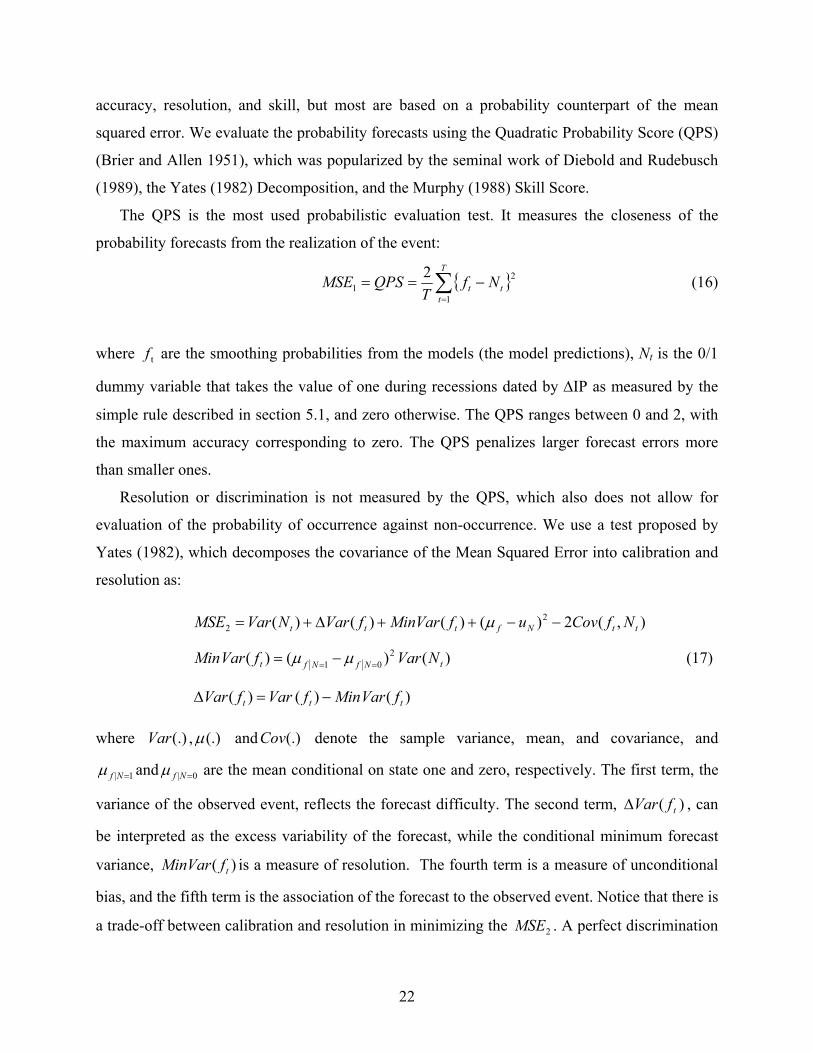
accuracy, resolution, and skill, but most are based on a probability counterpart of the mean

squared error. We evaluate the probability forecasts using the Quadratic Probability Score (QPS)

(Brier and Allen 1951), which was popularized by the seminal work of Diebold and Rudebusch

(1989), the Yates (1982) Decomposition, and the Murphy (1988) Skill Score.

The QPS is the most used probabilistic evaluation test. It measures the closeness of the

probability forecasts from the realization of the event:

∑=

−==T

t

tt NfT

QPSMSE1

2

1

2 (16)

where tf are the smoothing probabilities from the models (the model predictions), Nt is the 0/1

dummy variable that takes the value of one during recessions dated by ΔIP as measured by the

simple rule described in section 5.1, and zero otherwise. The QPS ranges between 0 and 2, with

the maximum accuracy corresponding to zero. The QPS penalizes larger forecast errors more

than smaller ones.

Resolution or discrimination is not measured by the QPS, which also does not allow for

evaluation of the probability of occurrence against non-occurrence. We use a test proposed by

Yates (1982), which decomposes the covariance of the Mean Squared Error into calibration and

resolution as:

),(2)()()()( 2

2 ttNfttt NfCovufMinVarfVarNVarMSE −−++Δ+= μ

)()()( 2

01 tNfNft NVarfVarMin == −= μμ (17)

)()()( ttt fVarMinfVarfVar −=Δ

where (.)Var , (.)μ and (.)Cov denote the sample variance, mean, and covariance, and

1| =Nfμ and 0| =Nfμ are the mean conditional on state one and zero, respectively. The first term, the

variance of the observed event, reflects the forecast difficulty. The second term, )( tfVarΔ , can

be interpreted as the excess variability of the forecast, while the conditional minimum forecast

variance, )( tfMinVar is a measure of resolution. The fourth term is a measure of unconditional

bias, and the fifth term is the association of the forecast to the observed event. Notice that there is

a trade-off between calibration and resolution in minimizing the 2MSE . A perfect discrimination

23

would imply miscalibrated forecasts given that it attains at the constant forecast

)0)(( =tfMinVar that results in a zero correlation between the forecast and the observed event.

On the other hand, a high degree of calibration implies only a fair degree of discrimination.

Finally, we also use Murphy’s decomposition of the Skill Score )( 4MSE . The basic skill

score compares the accuracy of the forecast with the constant forecast of the mean of tN :

)/(1 314 MSEMSEMSE −=

(18)

where ∑=

−=T

t

NtNTMSE1

2

3 2 μ is the benchmark forecast. The skill score is 1 for perfect

forecasts, 0 if the forecast is only as accurate as the benchmark forecast, and negative if the

forecast is less accurate than the reference. Murphy (1988) decomposes the skill score as:

222

5 ]/)[()]/(),([)],([ NNfNftttt SDSDSDfNCorrfNCorrMSE μμ −−−−= (19)

where (.)Corr and (.)SD stand for correlation and standard deviation, respectively. The first

term, the squared correlation between the forecast and the IP-dated recessions, is a measure of

resolution, which is high if the forecasts associated with the occurrence are generally higher than

the forecasts associated with nonoccurrence. The second term is the ‘conditional bias,’ and it

evaluates how well the standard deviation of the forecasts reflects the lack of perfect correlation.

The third term is the ‘unconditional bias’, and it measures how close the average forecast

matches the mean of the observed event. Note that the second and third terms are nonnegative,

which implies that the first term would be a measure of the forecast skill if the bias could be

eliminated.

Table 7 compares the accuracy of different models in predicting the IP-dated recessions,

using the Quadratic Probability Score. The table shows the forecast horizons in which the models

perform best in the short run, medium run, and long run, which are found to be at 3, 15, and 22

months, respectively. The level (Model 1) and the slope (Model 3) of the yield curve produce the

most accurate forecasts at the 15-month horizon, while the curvature (Model 2), the yield factor

(Model 4), and the yield-economic factor (Model 5) do best at the 22-month horizon. None of the

models perform as well in the short run. The joint dynamic factor model of the yield and the

economy (Model 5) displays the best accuracy at any horizon, with QPS values less than half of

24

the non-factor models. Our yield-only factor model (Model 4) displays the second best

performance. At the 22-month horizon, Models 5 and 4 have QPS = 0.209 and QPS = 0.362,

respectively, while the term spread (Model 3) has QPS=0.549. The worst accuracy is again for

the curvature (Model 2), with its lowest QPS = 1.088 (22-month horizon), while the level (Model

1) has its lowest QPS=0.805 (15-month).

Notice that the benchmark forecast, 3MSE , which is the constant forecast of the mean of the

observed event, ranges between 0.28-0.29. Thus, with the exception of Model 5, all the other

models have no advantage at any horizon compared to the benchmark forecast. This poor

performance is not conveyed by the QPS values, which show a fair accuracy for the models. The

source of the forecast inaccuracy can be examined using Murphy’s decomposition of the skill

score (Table 8). Model 5 is the only one that displays a positive skill score (from horizon 14 to

24). The main contributor of its superior performance is its larger correlation with the business

cycle dating, although the biases are also very small. The other models have negative skill at any

horizon. In particular, the forecasts from the level and curvature of the yield curve (Models 1 and

2) have large conditional bias and very low resolution. The term spread (Model 3) and the yield-

only factor (Model 4) models have high resolution at the 15 and 22-month horizons, but this

advantage is offset by their high conditional and unconditional biases. In particular, the model

that uses the popular term spread shows a reasonable degree of resolution (Table 8 column 4).

The tests indicate that the main weakness of the spread model is the high variability of its

forecasts, in addition to a relative large unconditional bias, which together imply a high degree of

miscalibration.

The forecasting performance in terms of resolution can be examined in more detail in Table

9, which shows Yates’ decomposition. For any horizon, Model 5 displays the lowest mean

squared error compared to the other models. The decomposition shows that this performance is

achieved due to the small unconditional bias of this model, 2)( Nf μμ − and the low excess

variability of the forecast, )( tfVarΔ . In addition, the conditional minimum value of forecast

variance, which reflects forecast discrimination with respect to times of occurrence and non-

occurrence of the event, is also the smallest for Model 5. The lowest MSE2 = 0.102 for Model 5

is achieved at horizon 22. This value is less than half of the MSE2 for all the univariate models at

25

any horizon. Model 4 also displays a good forecasting performance, especially at longer

horizons, achieving a good balance between resolution and calibration.

Overall, the tests suggest that all models of the yield curve perform best at leads of at least 15

months. Although the QPS shows that the models generally have reasonable accuracy, with the

exception of Model 5 the other models have very poor skill. On the other hand, Model 5 is well

calibrated and has positive skill score (forecasts better than the benchmark constant forecast). In

addition, the probabilities from Model 5 have effective information with respect to the event

occurrence, showing the highest discrimination power – the highest resolution and the lowest

conditional and unconditional biases, compared to the other models. Moreover, it has a better

balance between accuracy and resolution, leading to the smallest MSE.

In summary, we find that the components of the yield curve have useful information to

forecast recession and expansions. Although the popular term spread model has a reasonable

forecasting performance, the proposed factor models that use information of the whole yield

curve and of the economy exhibit superior predictive value to anticipate the beginning and end of

recessions. Using information from the yield curve only as in Model 4 leads to the second best

forecast performance, but the results of Model 5 shows that a substantial incremental predictive

value is achieved when the interrelationship between the bonds market and the economy are

considered.

7. Out-of-Sample Forecasting Analysis

The out-of-sample forecasting performance of alternative models for future values of the

industrial production growth is examined in this section. In addition to revised data, we also use

real-time data for Industrial Production obtained from the Federal Reserve Bank of Philadelphia.

These are the unrevised series as available at any given date in the past instead of the revised

data currently available. Industrial production has been substantially revised over the period

considered.

We consider three models to examine the usefulness of the information of the components of

the yield curve in predicting the growth rate of Industrial Production. Model 6 uses lags of the

slope and lags of Industrial Production itself. Model 7 uses lags of the level, curvature, and slope

of the yield curve in addition to lags of Industrial Production. Finally, we estimate a model that

includes lags of the yield curve factor extracted from the Markov-switching dynamic bifactor

26

yield-economy model in addition to lags of Industrial Production (Model 8). The lags for each

model are selected using Akaike, Schwarz and Hannan-Quinn criteria. The best specifications for

the autoregressive model of the growth of Industrial Production are the following:

Model 6: ttttt uTIPIPIP 110342110 ++Δ+Δ+=Δ −−− ββββ

Model 7: ttttttt uCLTIPIPIP 210510410342110 ++++Δ+Δ+=Δ −−−−− δδδδδδ

Model 8: tttttt uYFYFIPIPIP 314410342110 +++Δ+Δ+=Δ −−−− γγγγγ

Variables that exhibit high power in explaining the linear long-run variance of output may be

less important in specific situations. In fact, the largest errors in predicting output occur around

business cycle turning points. Thus, we choose to investigate the period before, during, and after

the 2001 recession, which will allow analysis of the ability of the models in predicting in an out-

of-sample real time exercise the substantial fall and recovery in the rate of growth of industrial

production during this phase.17

The models are first estimated using data from 1971:08 to 1999:12 and then recursively re-

estimated for each month for the period starting in 2000:1 and ending in 2003:12. We use the in-

sample estimates to generate h-step ahead forecasts in real time, using only collected real time

realizations of industrial production as first released at each month for this analysis. We consider

forecast horizons from 1 to 10 months, 10,...,1=h . The loss functions are evaluated using h-step

ahead forecast errors obtained through a recursive forecasting scheme. We consider three loss

functions: the root mean squared error (RMSE), Theil inequality coefficient (THEIL) and the

LINLIN asymmetric loss function of Granger (1969):

∑+

+=

Δ−Δ=RT

Tt

tt IPPIR

RMSE1

2)ˆ(1

17 This is the last recession phase for which both the peak and the trough are known at the time this paper was

written.

27

∑∑

∑+

+=

+

+=

+

+=

Δ+Δ

Δ−Δ=

RT

Tt

t

RT

Tt

t

RT

Tt

tt

IPR

PIR

IPPIR

THEIL

1

2

1

2

1

2

1ˆ1

)ˆ(1

∑+

+=

Δ−ΔΔ−Δ−+Δ−ΔΔ−Δ=RT

Tt

tttttttt IPPIbIPPIIIPPIaIPPIIR

LINLIN1

|ˆ|]ˆ(1[|ˆ|)ˆ(1

where T and R denote the number of observations in the estimation and forecast samples,

respectively, and tPI ˆΔ is the forecast and tIPΔ is the observation. (.)I is the standard indicator

function that takes the value of 1 if the forecast error is positive and takes the value of 0 if the

forecast error is negative, and 3,1 == ba . Notice that although LINLIN is linear on each side of

the origin, negative errors are penalized differently from positive errors because the lines have

different slopes on each side of the origin. The ratio a/b measures the cost of underpredicting

relative to the cost of overpredicting. We consider the loss associated with a negative error three

times as much as the loss associated with a positive error of the same magnitude.

Table 10 summarizes the results of the out-of sample forecast performance of the models in

real time. For all considered forecast horizons, the model that includes lags of the extracted

yield-economy factor (Model 8) does better than the other models with respect to each loss

function, and its advantage increases for longer horizons. Model 8 also performs relatively better

when we consider the asymmetric loss function that penalizes negative errors more than the

positive ones.

We repeat the same exercise using revised Industrial Production data in order to evaluate the

models forecasting performance in terms of what actually happened to the economy rather than

in real time. The results are reported in Table 11. Once again, for all horizons considered, Model

8 outperforms the alternative ones. This is especially the case for horizons longer than six, for

which the already superior predictive ability of Model 8 increases substantially. For example, the

asymmetric loss function LINLIN at h = 10 for Model 8 is 55% the value for Model 7 and 61%

the value for Model 6.

28

8. Conclusion

We propose a new model of the yield curve that uses information from the entire curve and of its

interrelationship with the economy. The multivariate bi-factor model follows two separate

Markov processes, each representing phases of the bonds markets and of the business cycle. The

framework allows direct analysis of the lead-lag relationship between the cyclical phases of these

two sectors. We use the model to forecast the beginning and end of future recessions and future

projections of industrial production growth at the monthly frequency.

The results show a strong correlation between the real economy and the bonds market. The

yield factor extracted from the interrelationship between both sectors has a superior ability to

anticipate economic recessions compared to alternative frameworks. In particular, it predicts the

beginning and end of all recessions in the sample studied with no false peaks or troughs and no

missed turns. In addition, the yield-economy factor model is well calibrated and exhibits a high

discrimination power. Its balance between accuracy and resolution yields a small mean squared

error compared to alternative models. The proposed model also outperforms alternative

specifications in terms of linear time series forecasting.

In summary, we find that the components of the yield curve – especially the term spread –

have useful information to forecast recessions and expansions and future projections of industrial

production growth. However, the proposed nonlinear model reduces the dimensionality of the

information on the yield curve down to one state variable that exhibits substantial incremental

predictive value compared to each of the components individually or even all the components

combined in a linear regression, especially when this unobserved variables is combined with

information on the economic activity.

We conclude that several attributes lead to the better predictive performance of the model:

the use of combined information from the entire yield curve in a latent factor, the extraction of

the yield factor based on the interrelationship of the yield curve with the real economic activity,

and the flexibility of the model, which allows for nonlinearities and asymmetries in the cyclical

phases of the bond markets and of the business cycle, as represented by the Markov processes.

29

References

Andrews, D.W.K., 1993, “Tests for Parameter Instability and Structural Change with Unknown

Change Point,” Econometrica, July, 61:4, 821–56.

Andrews, D.W.K. and W. Ploberger, 1994, “Optimal Tests When a Nuisance Parameter is

Present Only under the Alternative.” Econometrica, 62:6, pp. 1383–414.

Ang, A., Piazzesi, M., 2003, “A No-Arbitrage Vector Autoregression of Term Structure

Dynamics with Macroeconomic and Latent Variables,” Journal of Monetary Economics, 50,

745–787.

Ang, A., Piazzesi, M., Wei, M., 2006, “What Does the Yield Curve Tell us About GDP

Growth?” Journal of Econometrics, 127, 359-403.

Bai, J., 1997, “Estimating Multiple Breaks One at a Time,” Econometric Theory, 13, 315-352.

Bai, J. and P. Perron, 1998, “Estimating and Testing Linear Models with Multiple Structural

Changes, Econometrica, 66, 47-78.

Balduzzi, P., G. Bertola, and S. Foresi, 1997, “A Model of Target Changes and the Term

Structure of Interest Rates,” Journal of Monetary Economics, 39, 2, 223-249.

Bernadell, C., J. Coche, and K. Nyholm, 2005, “Yield Curve Prediction for the Strategic

Investor,” European Central Bank Working Paper 472.

Brier, G.W. and R.A. Allen, 1951, “Verification of Weather Forecasts;” in: T.F. Malone (ed.)

Compendium of Meteorology; American Meteorology. Soc. 841-848.

Chauvet, M., 1998/1999, “Stock Market Fluctuations and the Business Cycle,” Journal of

Economic and Social Measurement, 25, 235-258.

Chauvet and Potter, 2002, “Predicting Recessions: Evidence from the Yield Curve in the

Presence of Structural Breaks,” Economics Letters, 77, 2, 245-253.

Chauvet and Potter, 2005, “Forecasting Recessions Using the Yield Curve,” with S. Potter,

Journal of Forecasting, 24, 2, 77-103.

Chen, L., 1996, “Stochastic Mean and Stochastic Volatility – A Three Factor Model of the Term

Structure of Interest Rates and its Application to the Pricing of Interest Rate Derivatives,”

Blackwell Publishers, London.

Chib, S., 1998, “Estimation and Comparison of Multiple Change-Point Models,” Journal of

Econometrics, 86, 22, 1998, 221-241.

30

Dai, Q., Singleton, K., 2000, “Specification Analysis of Affine Term Structure Models,” Journal

of Finance, 55, 1943–1978.

Dickey, D.A. and W.A. Fuller, 1979, “Distribution of the Estimators for Autoregressive Time

Series with a Unit Root,” Journal of the American Statistical Association, 74, 366, 427-431.

Diebold, F.X. and G.D. Rudebusch, 1989, “Scoring the Leading Indicators,” Journal of Business,

62, 3, 369-91.

Diebold, F.X. and C. Li, 2006, “Forecasting the Term Structure of Government Bond Yields,”

Journal of Econometrics, 130, 337-364.

Diebold, F.X., G.D. Rudebusch, and B. Aruoba, 2006, “The Macroeconomy and the Yield

Curve,” Journal of Econometrics, 131, 309–338.

Dotsey, M., 1998, “The Predictive Content of the Interest Rate Term Spread for Future

Economic Growth,” Federal Reserve Bank of Richmond, Economic Quarterly, 84, 31-51.

Duffie, D., Kan, R., 1996, “A Yield-Factor Model of Interest Rates, Mathematical Finance, 6,

379–406.

Estrella, A. and G. Hardouvelis, 1991, “The Term Structure as a Predictor of Real Economic

Activity,” Journal of Finance, 46, 2, 555-576.

Estrella, A. and F.S. Mishkin, 1998, “Predicting U.S. recessions: Financial Variables as Leading

Indicators,” The Review of Economics and Statistics, 80, 45-61.

Estrella, A., A.P. Rodrigues, and S. Schich, 2003, “How Stable is the Predictive Power of the

Yield Curve? Review of Economics and Statistics, 85, 3, 629-644.

Friedman, B.M. and K.N. Kuttner, 1998, “Indicator Properties of the Paper-Bill Spread: Lessons

from Recent Experience,” The Review of Economics and Statistics, 80, 34-44.

Giacomini, R. and B. Rossi, 2006, “How Stable is the Forecasting Performance of the Yield

Curve for Output Growth?” Oxford Bulletin of Economics and Statistics 68(s1), December,

783-795.

Granger, C.W.J., 1969, “Prediction with a Generalized Cost of Error Function,” Operational

Research Quarterly, 20, 199–207.

Gurkaynak, R.S., B. Sack, and J.H. Wright, 2007, “The U.S. Treasury Yield Curve: 1961 to the

Present.” Journal of Monetary Economics, 24, 8, 2291-2304.

Hamilton, J.D., 1989, “A New Approach to the Economic Analysis of Nonstationary Time Series

and Business Cycles,” Econometrica ,57, 357-384.

31

Hamilton, J.D. and D.H. Kim, 2002, “A Re-Examination of the Predictability of Economic

Activity Using the Yield Spread,” Journal of Money, Credit and Banking, 34, 340–344.

Harvey, C., 1988, “The Real Term Structure and Consumption Growth,” Journal of Financial

Economics 22, 305-334.

Harvey, C., 1989, “Forecasting Economic Growth with the Bond and Stock Markets,” Financial

Analysts Journal, 38-45.

Haubrich, J.G. and A.M. Dombrosky, 1996, “Predicting Real Growth Using the Yield Curve,”

Federal Reserve Bank of Cleveland Economic Review, 32, 1, 26-34.

Kim, C.-J., 1994, “Dynamic Linear Models with Markov-Switching,” Journal of Econometrics,

60, 1-22.

Knez, P.J., R. Litterman, J. Scheinkman, 1994, “Explorations Into Factors Explaining Money

Market Returns,” Journal of Finance, 49, 5, 1861-82.

Litterman, R. and J. Scheinkman, 1991, “Common Factors Affecting Bond Returns,” Journal of

Fixed Income, 1, 1, 54-61.

McConnell, M. and G. Perez-Quiros, 2000, “Output Fluctuations in the United States: What Has

Changed Since the Early 1980s?”, American Economic Review, 90, 1464-1476.

Murphy, A. 1988, “Skill Scores based on the Mean Square Error and their Relationships to the

Correlation Coefficient,” Monthly Weather Review, 116, 2417-2424.

Nelson, C.R. and A.F. Siegel, 1987, “Parsimonious Modeling of Yield Curves,” Journal of

Business, 60, 473–489.

Nyholm, K., 2007, “A New Approach to Predicting Recessions,” Economic Notes, 36, 27-42.

Phillips, P. and P. Perron, 1988, “Testing for a Unit Root in Time Series Regression,”

Biometrika, 75, 2, 335-346.

Perron, P., 1989, “The Great Crash, the Oil Shock and the Unit Root Hypothesis,” Econometrica,

57, 1361-1401.

Senyuz, Z. (2008) "Essays on Nonlinear Modeling of Real and Financial Markets with

Applications to U.S. and International Data", UCR Ph.D. Dissertation.

Stock, J.H. and M.W. Watson, 2003, “Forecasting Output and Inflation: The Role of Asset

Prices,” Journal of Economic Literature, 41, 3, 788-829.Journal of Monetary Economics 24(8),

November 2007, 2291-230

Stock, J. and M. Watson, 1989, “New Indices of Coincident and Leading Indicators,” In O.

Blanchard and S. Fischer ed. NBER Macroeconomic Annual, Cambridge, MIT Press

32

Wright, J., 2006, “The Yield Curve and Predicting Recessions,” Federal Reserve Board,

Washington, Working Paper no. 2006-7.

Yates, J.F. (1982), “External Correspondence: Decompositions of the Mean Probability Score,”

Organizational Behavior and Human Performance, 30,132-156.

33

Table 1 – Results of Structural Break Tests

Breakdate

Interval – Yield

Level Curvature Slope Industrial

Production

Components Mean Variance Mean Variance Mean Variance Mean Variance

1980:05-1981:08 - 1980:05*** - 1980:08** 1982:01** 1980:06***

1981:02**

1981:08***

- 1983:12**

1990:06-1990:12 1990:11*** - 1990:6** - - - - -

* significant at the 10% level, ** significant at the 5% level, *** significant at the 1% level.

Table 2: Maximum Likelihood Estimates for the Univariate Markov Switching (MS)

Model for ΔIP

Parameter Estimates

α1 4.13

(0.16)

α0 -4.24

(0.42)

p11 0.99

(0.01)

p00 0.93

(0.03)

σ2IP 8.28

(0.57)

LogL -395.12

Standard errors in parentheses

34

Table 3: Maximum Likelihood Estimates of the Univariate and

Multivariate MS Models of the Yield Curve

Parameters Univariate Models Multivariate

Yield Factor

Level Curvature Slope Model

*

1

t<α

10.12

(0.17) 1.27

(0.67)

1.99

(0.08)

0.59

(0.162)

*

0

t<α 5.48

(0.10)

0.190

(0.05)

-0.96

(0.12)

-0.42

(0.15)

*

1

t≥α

5.44

(0.06)

0.327

(0.03)

3.04

(0.06) -

*

0

t≥α 3.03

(0.12)

-1.27

(0.07)

0.89

(0.06) -

*,2 t<ησ

2.60

(0.18)

0.25

(0.02)

0.63

(0.07) -

*,2 t≥ησ 0.54

(0.05)

0.32

(0.03)

0.37

(0.03) -

11p 0.98

(0.01)

0.94

(0.03)

0.97

(0.02)

0.93

(0.04)

00p 0.99

(0.01)

0.97

(0.01)

0.96

(0.01)

0.96

(0.02)

φ - - - 0.89

(0.03)

Levelλ - - - 0.015

(0.00)

Curvatureλ - - - -0.10

(0.02)

Slopeλ - - - -0.27

(0.01)

Leveld - - - 0.99

(0.00)

Curvatured - - - 0.95

(0.02)

Sloped - - - -0.91

(0.04)

2

,Leveleσ - - - 0.04

(0.00)

2

,Curvatureeσ - - - 0.37

(0.01)

2

,Slopeeσ - - - 0.01

(0.00)

LogL -395.12 25.23 -91.89 1680.66

Asymptotic standard errors in parentheses correspond to the diagonal elements of the inverse hessian

obtained through numerical calculation. The variance of the single factor is set to one for normalization.

35

Table 4: Maximum Likelihood Estimates of the Joint Bi-Factor

Model of the Yield Curve and the Economy

Parameters Yield Factor Economic

Factor

1α 0.596

(0.184)

0.802

(0.068)

0α -0.374

(0.136)

-0.934

(0.100)

11p 0.930

(0.041)

0.877

(0.045)

00p 0.971

(0.021)

0.962

(0.017)

2

ησ 1 0.856

(0.029)

φ 0.883

(0.011)

0.885

(0.017)

IPλ - 1

Levelλ 0.015

(0.002) -

Curvatureλ -0.274

(0.009)

-

Slopeλ -0.102

(0.015)

-

2

,Leveleσ 0.043

(0.001)

-

2

,Curvatureeσ 0.371

(0.010) -

2

,Slopeeσ 0.002

(0.582)

-

θ 0.038

(0.018)

-0.116

(0.009)

Curvatured 0.946

(0.014) -

Log L 367.212

Asymptotic standard errors in parentheses

36

Table 5 - Turning Point Signals of the Reference Cycle (IP)

Turning Point

IP

Model 1

Level

Model 2 Curvature

Model 3

Slope

Model 4 Yield-only

Model 5 Yield-

Economy

6 peaks

In-sample 1974:09 - -38 -19 -22 -221980:03 -21 -14 -19 -31 -221981:11 - - -14 -17 -171990:12 -31 - -27 -27 -292001:02 - -3 - -13 -13

Out-of-Sample Real Time

2007:12 -25 -4 -34 -34 -35 5 Troughs

Turning Point

IP

Model 1

Level

Model 2 Curvature

Model 3

Slope

Model 4 Yield-only

Model 5 Yield-

Economy

In-Sample 1975:11 - -9 -12 -4 -161981:03 - - -11 -13 -131983:04 - - -19 -18 -241991:10 -13 - -9 -23 -232002:05 -9 - -11 -21 -19

Out-of-Sample Real Time

Not announced* - - - Yes Yes

The criterion adopted to determine turning points in cols. (2)-(5) is if the smoothed probability of state 0 is equal or

greater than 0.5: P(St=0|IT) ≥ 0.5. The minus sign refers to the lead in which the models anticipate the recession

dates. An increase in the probabilities above 50% more than 4 years before a recession is not considered a recession

signal, but a false signal.

The last row of both tables refers to the models recursively estimated using real time data from 2004:01 to 2007:12.

(*) The trough of the 2007-2009 had not been announced at the time the paper was written, in December 2008.

37

Table 6 - Turning Point Signal Errors of the Reference Cycle (IP)

Turning Point

Evaluation

Model 1

Level

Model 2 Curvature

Model 3

Slope

Model 4 Yield-only

Model 5 Yield-

Economy

6 Peaks

Correct TP 3 4 5 6 6

Missed TP 3 2 1 0 0

False TP 0 2 2 2 0

TP Error 3 4 3 2 0

5 Troughs*

Correct TP 2 1 4 5 5

Missed TP 3 4 1 0 0

False TP 0 2 1 2 0

TP Error 3 6 2 2 0

(*) It does not include the trough for the current recession (2007-2009), which Models 4 and 5 have already

signaled.

Correct TP refers to prediction of a turning point when one does occur. Missed TP refers to prediction of no turning

point when one does occur. False TP refers to prediction of a turning point when one does not occur. TP error refers

to the total of Missed and False TP. A perfect forecast is when TP error is zero.

Table 7 - Evaluation of Turning Point Forecasts of the Reference Cycle (IP)

Using the Quadratic Probability Score (MSE1)

Forecast

MSE3 MSE1

Horizon Model 1

Level Model 2

Curvature Model 3

Slope Model 4

Yield Only

Model 5 Yield-

Economy

3-month 0.278 0.977 1.105 0.919 0.790 0.552

15-month 0.286 0.805 1.092 0.549 0.436 0.259

22-month 0.290 0.808 1.088 0.604 0.362 0.209

38

Table 8 – Skill Score - Murphy Decomposition (MSE5)

Models Forecast Horizon

Total Score Squared

Correlation Conditional

Bias Uncond.

Bias

Model 1 3 -2.502 0.003 1.561 0.944

15 -1.888 0.070 1.081 0.876

22 -1.777 0.058 1.073 0.761

Model 2 3 -2.967 0.001 1.689 1.280

15 -2.951 0.000 1.582 1.369

22 -2.771 0.000 1.449 1.322

Model 3 3 -2.281 0.000 1.712 0.569

15 -0.972 0.219 0.683 0.507

22 -1.067 0.141 0.787 0.422

Model 4 3 -1.835 0.026 1.436 0.425

15 -0.555 0.195 0.355 0.396

22 -0.233 0.299 0.210 0.322

Model 5 3 -0.982 0.001 0.904 0.079

15 0.094 0.299 0.139 0.065

22 0.295 0.396 0.062 0.039

Table 9 - Evaluation of Turning Point Forecasts of the Reference Cycle (IP)

Using Yates’ Decomposition (MSE2)

Models Forecast Horizon

MSE2 Var (Nt) ΔVar (ft) Min Var

(ft) (μf - μN)

2 2*cov(ft, Nt)

Model 1 3 0.488 0.139 0.236 0.001 0.132 0.019

15 0.401 0.139 0.230 0.007 0.122 0.098

22 0.403 0.145 0.234 0.003 0.111 0.090

Model 2 3 0.553 0.139 0.221 0.000 0.179 -0.014

15 0.551 0.139 0.217 0.003 0.191 -0.001

22 0.548 0.145 0.215 0.002 0.192 0.006

Model 3 3 0.458 0.139 0.236 0.000 0.079 -0.003

15 0.272 0.139 0.209 0.024 0.071 0.172

22 0.300 0.145 0.229 0.003 0.061 0.139

Model 4 3 0.396 0.139 0.143 0.007 0.059 -0.047

15 0.215 0.139 0.087 0.063 0.055 0.130

22 0.179 0.145 0.121 0.025 0.047 0.160

Model 5 3 0.276 0.139 0.120 0.000 0.011 -0.006

15 0.124 0.139 0.079 0.039 0.009 0.143

22 0.102 0.145 0.093 0.019 0.006 0.161

Nt is the 0/1 dummy that takes the value 0 if the smoothed probability of state 0 for ΔIP is equal to or greater than

0.5: P(St=0|IT) ≥ 50%. Yates’ decomposition is: MSE2 = Var (Nt)+ Δ Var (ft) + Min Var(ft)+ (μf - μN)2- 2Cov (ft, Nt).

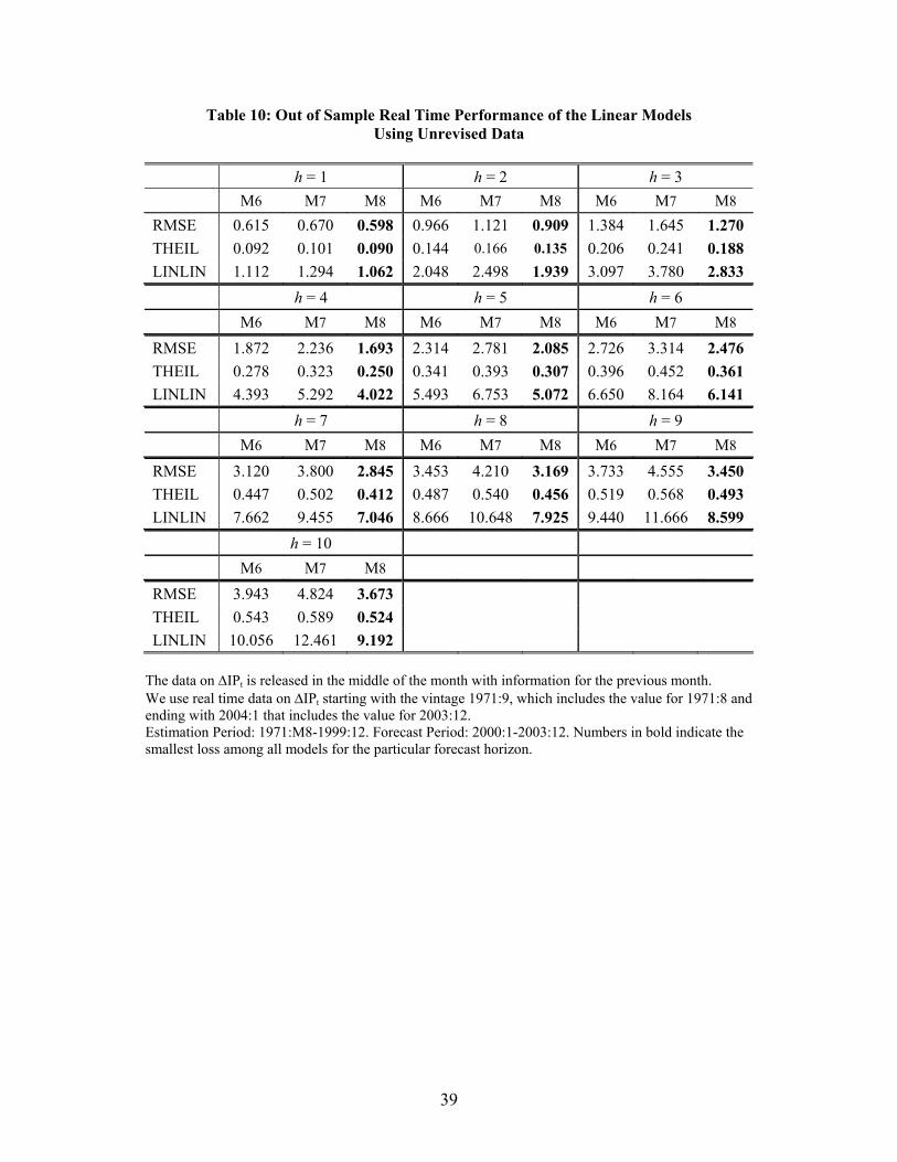
39

Table 10: Out of Sample Real Time Performance of the Linear Models

Using Unrevised Data

h = 1 h = 2 h = 3

M6 M7 M8 M6 M7 M8 M6 M7 M8

RMSE 0.615 0.670 0.598 0.966 1.121 0.909 1.384 1.645 1.270

THEIL 0.092 0.101 0.090 0.144 0.166 0.135 0.206 0.241 0.188

LINLIN 1.112 1.294 1.062 2.048 2.498 1.939 3.097 3.780 2.833

h = 4 h = 5 h = 6

M6 M7 M8 M6 M7 M8 M6 M7 M8

RMSE 1.872 2.236 1.693 2.314 2.781 2.085 2.726 3.314 2.476

THEIL 0.278 0.323 0.250 0.341 0.393 0.307 0.396 0.452 0.361

LINLIN 4.393 5.292 4.022 5.493 6.753 5.072 6.650 8.164 6.141

h = 7 h = 8 h = 9

M6 M7 M8 M6 M7 M8 M6 M7 M8

RMSE 3.120 3.800 2.845 3.453 4.210 3.169 3.733 4.555 3.450

THEIL 0.447 0.502 0.412 0.487 0.540 0.456 0.519 0.568 0.493

LINLIN 7.662 9.455 7.046 8.666 10.648 7.925 9.440 11.666 8.599

h = 10

M6 M7 M8

RMSE 3.943 4.824 3.673

THEIL 0.543 0.589 0.524

LINLIN 10.056 12.461 9.192

The data on ΔIPt is released in the middle of the month with information for the previous month.

We use real time data on ΔIPt starting with the vintage 1971:9, which includes the value for 1971:8 and

ending with 2004:1 that includes the value for 2003:12.

Estimation Period: 1971:M8-1999:12. Forecast Period: 2000:1-2003:12. Numbers in bold indicate the

smallest loss among all models for the particular forecast horizon.

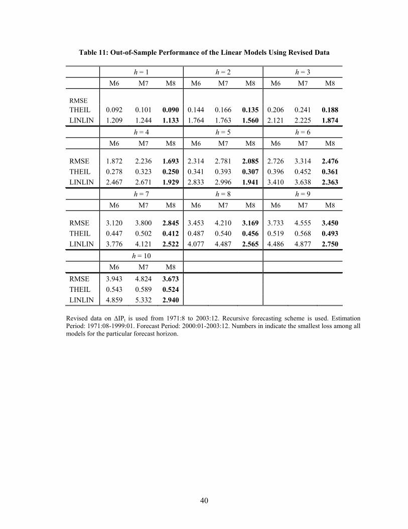
40

Table 11: Out-of-Sample Performance of the Linear Models Using Revised Data

h = 1 h = 2 h = 3

M6 M7 M8 M6 M7 M8 M6 M7 M8

RMSE

THEIL 0.092 0.101 0.090 0.144 0.166 0.135 0.206 0.241 0.188

LINLIN 1.209 1.244 1.133 1.764 1.763 1.560 2.121 2.225 1.874

h = 4 h = 5 h = 6

M6 M7 M8 M6 M7 M8 M6 M7 M8

RMSE 1.872 2.236 1.693 2.314 2.781 2.085 2.726 3.314 2.476

THEIL 0.278 0.323 0.250 0.341 0.393 0.307 0.396 0.452 0.361

LINLIN 2.467 2.671 1.929 2.833 2.996 1.941 3.410 3.638 2.363

h = 7 h = 8 h = 9

M6 M7 M8 M6 M7 M8 M6 M7 M8

RMSE 3.120 3.800 2.845 3.453 4.210 3.169 3.733 4.555 3.450

THEIL 0.447 0.502 0.412 0.487 0.540 0.456 0.519 0.568 0.493

LINLIN 3.776 4.121 2.522 4.077 4.487 2.565 4.486 4.877 2.750

h = 10

M6 M7 M8

RMSE 3.943 4.824 3.673

THEIL 0.543 0.589 0.524

LINLIN 4.859 5.332 2.940

Revised data on ΔIPt is used from 1971:8 to 2003:12. Recursive forecasting scheme is used. Estimation

Period: 1971:08-1999:01. Forecast Period: 2000:01-2003:12. Numbers in indicate the smallest loss among all

models for the particular forecast horizon.

41

Figure 1: Empirical Proxies for the Level, Slope, and Curvature of the Yield Curve and

NBER-Dated Recessions

-4

0

4

8

12

16

75 80 85 90 95 00 05

LEVEL CURVATURE SLOPE

Figure 2: The Term Spread and NBER-Dated Recessions

-3

-2

-1

0

1

2

3

4

5

55 60 65 70 75 80 85 90 95 00 05

42

Figure 3: Smoothed Probabilities of Recession from Growth Rate

of Industrial Production (IP-Dated Recessions)

0.0

0.2

0.4

0.6

0.8

1.0

75 80 85 90 95 00 05

43

Figure 4: Level, Smoothed Probabilities of High Level State,

and IP-Dated Recessions (Shaded Area)

0.0

0.2

0.4

0.6

0.8

1.0

2

4

6

8

10

12

14

75 80 85 90 95 00 05

Figure 5: Curvature, Smoothed Probabilities of Low Curvature State,

and IP-Dated Recessions (Shaded Area)

0.0

0.2

0.4

0.6

0.8

1.0

-2

-1

0

1

2

3

75 80 85 90 95 00 05

Figure 6: Slope and Smoothed Probabilities of Flat or Inverted Slope State

and IP-Dated Recessions

0.0

0.2

0.4

0.6

0.8

1.0

-4

-3

-2

-1

0

1

2

3

4

5

75 80 85 90 95 00 05

44

Figure 7: Smoothed Probabilities of High State for the Yield Curve Single Factor,

IP-Dated Recessions (Shaded Area)

0.0

0.2

0.4

0.6

0.8

1.0

75 80 85 90 95 00 05

45

Figure 8: Yield Curve Factor from Joint Bifactor Model of the Yield Curve

and the Economy and its Components. Shaded Areas are IP-Dated Recessions

-8

-4

0

4

8

12

16

75 80 85 90 95 00 05

Yield Factor LevelCurvature Slope

Figure 9: Smoothed Probabilities of the Yield Curve Factor from the Joint Model of the

Yield Curve and the Economy. Shaded Areas are IP-Dated Recessions

0.0

0.2

0.4

0.6

0.8

1.0

75 80 85 90 95 00 05