A Joint Count-Continuous Model of Travel Behavior with Selection Based on a

Multinomial Probit Residential Density Choice Model

Chandra R. Bhat (corresponding author) The University of Texas at Austin

Department of Civil, Architectural and Environmental Engineering 301 E. Dean Keeton St. Stop C1761, Austin TX 78712

Phone: 512-471-4535; Fax: 512-475-8744 Email: bhat@mail.utexas.edu

and King Abdulaziz University, Jeddah 21589, Saudi Arabia

Sebastian Astroza

The University of Texas at Austin Department of Civil, Architectural and Environmental Engineering

301 E. Dean Keeton St. Stop C1761, Austin TX 78712 Phone: 512-471-4535, Fax: 512-475-8744

Email: sastroza@utexas.edu

Raghuprasad Sidharthan Parsons Brinckerhoff

999 3rd Ave, Suite 3200, Seattle, WA 98104 Phone: 206-382-5289, Fax: 206-382-5222

E-mail: srprasad@utexas.edu

Mohammad Jobair Bin Alam King Abdulaziz University

Department of Civil Engineering P.O. Box 80204, Jeddah 21589, Saudi Arabia

Phone: +966-2-6402000 (Ext.: 51339), Fax: +966-2-6952179 Email: malam@kau.edu.sa

Waleed H. Khushefati

King Abdulaziz University Department of Civil Engineering

P.O. Box 80204, Jeddah 21589, Saudi Arabia Phone: +966-2-6402000 (Ext.: 51339), Fax: +966-2-6952179

Email: wkhushefati@kau.edu.sa

Original version July 2013 Revised version January 2014

ABSTRACT

This paper formulates a multidimensional choice model system that is capable of handling multiple

nominal variables, multiple count dependent variables, and multiple continuous dependent variables.

The system takes the form of a treatment-outcome selection system with multiple treatments and

multiple outcome variables. The Maximum Approximate Composite Marginal Likelihood

(MACML) approach is proposed in estimation, and a simulation experiment is undertaken to

evaluate the ability of the MACML method to recover the model parameters in such integrated

systems. These experiments show that our estimation approach recovers the underlying parameters

very well and is efficient from an econometric perspective. The parametric model system proposed

in the paper is applied to an analysis of household-level decisions on residential location, motorized

vehicle ownership, the number of daily motorized tours, the number of daily non-motorized tours,

and the average distance for the motorized tours. The empirical analysis uses the NHTS 2009 data

from the San Francisco Bay area. Model estimation results show that the choice dimensions

considered in this paper are inter-related, both through direct observed structural relationships and

through correlations across unobserved factors (error terms) affecting multiple choice dimensions.

The significant presence of self-selection effects (endogeneity) suggests that modeling the various

choice processes in an independent sequence of models is not reflective of the true relationships that

exist across these choice dimensions, as also reinforced through the computation of treatment effects

in the paper.

Keywords: multivariate dependency; self-selection; treatment effects; maximum approximate

composite marginal likelihood; land-use and built environment; travel behavior.

1

1. INTRODUCTION

A question that has received particular attention within the broad land use-transportation literature is

whether any effect of the built environment on travel demand is causal or merely associative (or

some combination of the two; see, for example, Bhat et al., 2009 and van Wee, 2009). Commonly

labeled as the residential self-selection problem, the underlying issue is that the data available to

assess the potential effects of land-use on travel patterns is typically of a cross-sectional nature. In

such observational data, the residential location of households and the travel patterns of household

members are jointly observed at a given point in time. Thus, the data reflects household residential

location preferences co-mingled with the travel preferences of the households. On the other hand,

from a policy perspective, the emphasis is on analyzing whether (and how much) a neo-urbanist

design (compact built environment design, high bicycle lane and roadway street density, good land-

use mix, and good transit and non-motorized mode accessibility/facilities) would help in reducing

motorized vehicle miles of travel (VMT). To do so, the conceptual experiment that reveals the “true”

effect of the built environment (BE) features of the residential location on travel patterns is the one

that randomly locates households in residential locations. The problem then, econometrically

speaking, is that the analyst has to extract out the “true” BE effect from a potentially non-randomly

assigned (to residential locations) observed cross-sectional sample. If the non-random assignment

can be completely captured by observed non-travel characteristics of households and the BE (such

as, say, poor households locating in areas with low housing cost), then a conventional travel model

accommodating the observed non-travel characteristics of households and the BE characteristics

would suffice to extract the “true” BE effect on travel. However, it is quite possible (if not likely)

that there are some antecedent characteristics of households that are not observed by the analyst and

that impact both residential location choice and travel behavior. For instance, a household whose

members have an overall auto inclination and a predisposition to enjoy private travel may locate

itself in a conventional neighborhood (low population density, low bicycle lane and roadway street

density, primarily single use residential land use, and auto-dependent urban design) and undertake

substantial auto travel, while a household whose members dislike driving and prefer non-motorized

and transit forms of travel may seek out neo-urbanist neighborhoods so they can pursue their

activities using non-motorized and transit modes of travel. Ignoring such self-selection effects in

residence choices can lead to a “spurious” causal effect of neighborhood attributes on travel, and

potentially lead to misinformed BE design policies.

2

Many different approaches have been proposed in the literature to account for residential

self-selection effects, a detailed review of which is beyond the scope of this paper (the reader is

referred to Bhat and Guo, 2007, Pinjari et al., 2007, Mokhtarian and Cao, 2008, Bohte et al., 2009,

van Wee, 2009, and Van Acker et al., 2011, 2012). In this paper, we accept the limitations of

traditional cross-sectional surveys and attempt to control for self-selection effects through

econometric instrumental variable techniques, and/or parametric distribution assumptions regarding

the unobserved factors. Many earlier efforts in the transportation literature have used such an

approach, which can also be used in combination with other approaches (see Chatman, 2009, Pinjari

et al., 2011 and de Abreu e Silva et al., 2012). In doing so, we provide important empirical

extensions of earlier works as well as methodological innovations, as discussed in the next section.

1.1. The Current Paper in the Context of Earlier Studies

As discussed by Bhat and Guo (2007), there are several challenges in analyzing the effects of BE

measures on travel behavior, even beyond the issue of residential self-selection, including the multi-

dimensional nature of the BE and travel behavior. In terms of travel behavior, the different

dimensions include motorized and non-motorized vehicle ownership by type, number of tours and

stops, time-of-day, route choice, and travel mode choice. The net impact on overall VMT patterns

will depend on the aggregation across the effects on individual travel dimensions. However, most

earlier studies on the effect of BE measures on travel, while considering residential self-selection,

focus directly (and solely) on the effect on vehicle miles of travel (see Zhang et al., 2012, Salon et

al., 2012, and Cao and Fan, 2012, which are but a few recent examples). There have also been

studies that consider residential self-selection and focus on BE effects on specific travel dimensions,

such as auto ownership, vehicle type, trip frequencies, bicycle ownership, activity durations, and

mode choice, though these have been relatively few and have focused on each dimension

individually (see Bhat and Eluru, 2009 and Handy and Krizek, 2012 for detailed reviews). On the

other hand, BE measures may have opposite effects on different dimensions characterizing the VMT

components. For instance, a neo-urbanist design at the residence end may decrease trip lengths, but

also increase the number of auto trips. As a result, a BE variable may appear to have no effect on

VMT, though that may be because of opposite effects on different components constituting VMT.

This is of relevance for policy, because the emissions per mile can be higher if a neo-urbanist design

increases the number of auto trips, which may more than compensate for the emissions decrease

3

because of a VMT decrease (see Sperry et al., 2012). Thus, there is a need to understand the

differential effects of BE on different travel dimensions, rather than simply examine an aggregate

effect on VMT or on an individual dimension of VMT. Further, the travel dimensions need to be

modeled jointly because, as elucidated by Van Acker et al. (2012) and Paleti et al. (2013), self-

selection need not be only through residential choice. For example, an auto-disinclined household

may own fewer motorized vehicles, make fewer auto tours, as well as drive shorter distances using

the car as the mode of transportation. As a consequence, any effect of the number of motorized

vehicles on auto travel and VMT will be moderated by the auto-disinclined nature of the household.

If some of the attributes associated with the auto-disinclined nature of the household are unobserved,

there is self-selection in auto travel and VMT based not only on residential choice but also based on

the number of motorized vehicles owned. This self-selection needs to be considered to obtain

accurate estimates of BE effects and auto-ownership on travel-related attributes. That is, residential

location may structurally affect motorized vehicle ownership and travel choices, and motorized

vehicle ownership may structurally affect travel choices, but underlying propensities for vehicle

ownership and travel choices may themselves affect residential location in the first place and

underlying propensities for travel may affect motorized vehicle ownership. The only way to

accurately reflect these impacts and capture the “bundling” of choices is to model the choice

dimensions together in a joint equations modeling framework that accounts for correlated

unobserved lifestyle (and other) effects as well as possible structural effects.1,2

1 In joint limited-dependent variable systems in which one or more dependent variables are not observed on a continuous scale, such as the joint system considered in the current paper that has discrete dependent and count variables (which we will more generally refer to as limited-dependent variables), the structural effects of one limited-dependent variable on another can only be in a single direction. That is, it is not possible to have correlated unobserved effects underlying the propensities determining two limited-dependent variables, as well as have the observed limited-dependent variables themselves structurally affect each other in a bi-directional fashion. This creates a logical inconsistency problem (see Maddala, 1983, page 119 for a good discussion). Intuitively, the propensities are the precursors to the actual observed variables, and, when both the decisions are co-determined, it is impossible to have both observed variables structurally affect one another. In the current paper, we estimate models with each possible structural direction impact, and choose the one that provides a better data fit (which also turns out to be the one that is conceptually intuitive). However, it is critical to note that, regardless of which directionality of structural effects comes out to be better (or even if both directions are not statistically significant), the system is a joint bundled system because of the correlation in unobserved factors impacting the underlying propensities.

2 Most earlier studies in the literature focus on the issue of controlling for self-selection when discussing the effects of BE variables on travel behavior. Less discussed is how the social environment may impact travel behavior. That is, it is possible that there are no self-selection effects in residential choice or other choices, but that individuals in close proximity get influenced by each other and so start exhibiting similar travel behaviors. Bhat and Dubey (2013) discuss a conceptual framework that identifies the many intervening effects that need to be controlled for when assessing BE effects, including social environment effects. They also propose a corresponding methodology for the case of the single

4

To be sure, there have been a few recent examples of a multi-dimensional modeling system

in the land use-transportation literature. These systems use a two-stage instrumental variables

approach (such as Vance and Hedel, 2007), or a full-information likelihood inference approach

(Brownstone and Golob, 2009, and Kim and Brownstone, 2013), or a structural equations approach

(Van Acker et al., 2012 and de Abreu e Silva et al., 2012), or a simulated maximum likelihood or a

simulated Bayesian inference approach (Eluru et al., 2010, Pinjari et al., 2011, Brownstone and

Fang, 2013). In the first (instrumental variable) approach, it can be a challenge to find good

instruments (Puhani, 2000). The rest of the approaches, while plausible, do become relatively

cumbersome in the presence of a mixture of dependent variables (such as continuous, nominal, and

count variables), and/or as the number of dimensions increases, as noted by earlier studies that use

these approaches (further, none of these multidimensional systems accommodate count variables). In

the current paper, we use the Maximum Approximate Composite Marginal Likelihood (MACML)

approach proposed by Bhat (2011) that, in a relatively simple and practical manner, provides a way

out to estimate multi-dimensional choice model systems. In this regard, the paper proposes the use of

Bhat’s MACML approach to estimate multi-dimensional systems with multiple nominal variables

and multiple count dependent variables in the multi-dimensional system. In addition to providing a

practical and very quick estimation approach, the approach is robust and yields consistent estimates

under a range of possible full joint distributions that characterize the high-order dependency of

endogenous variables in the multi-dimensional system. To our knowledge this is the first such

sample selection formulation and application in the econometrics literature. In particular, the sample

selection model takes the form of a treatment-outcome model with multiple treatments and multiple

outcomes, with several outcomes taking the form of count variables.

The parametric system proposed in this paper models residential choice as a discrete choice

among a multinomial set of four land-use density categories as defined by housing unit density

(housing units per square mile) within census blocks. This helps make the definition of choice

alternatives clear and manageable, and also alleviates the problem of strong multi-collinearity of

density with other BE characteristics that impact travel behavior. The use of density as the BE

measure of interest is quite common, and has been used in many earlier residential self-selection

travel behavior dimension for mode choice. However, we will not focus on these social environment effects in this paper that models multiple travel behavior dimensions simultaneously. But extending the literature to include self-selection

5

studies, including the recent studies of Kim and Brownstone (2013), Paleti et al. (2013), and Cao

and Fan (2012).3 The other endogenous variables in the system include the number of motorized

vehicles in the household (a count variable), the number of motorized auto vehicle tours across all

individuals in the household during the 24-hour period of the travel survey (another count variable),

the number of non-motorized tours across all individuals in the household (a third count variable),

and finally the continuous variable of average tour distance per auto tour.4

The key to our accommodation of count variables in the multi-dimensional system is the

recasting of a univariate count model as a restricted version of a univariate generalized ordered-

response probit (GORP) model, as discussed in Castro, Paleti, and Bhat or CPB (2012). In addition

to providing substantial flexibility to accommodate high or low probability masses for specific count

outcomes, the latent variable-based count specification provides a convenient mechanism to tie the

count outcomes with one another, and with the multinomial probit residential location choice model

and the continuous average trip distance per auto trip model.

2. MODEL STRUCTURE

In this section, we first discuss the formulation for each type of variable, and then formulate the

structure and estimation procedure for the multi-dimensional system.

2.1. Nominal Dependent Variables

considerations as well as social environment effects (when examining BE effects) is an important direction in land use-transportation research. 3 Interestingly, some earlier studies that use land-use density as the basis for residential location use density as a continuous variable in a linear regression model (for example, see Kim and Brownstone, 2013 and Brownstone and Golob, 2009). On the other hand, some other studies translate density into a nominal categorical variable in a multinomial choice model (for example, see Cao and Fan, 2012 and Paleti et al., 2013). There are advantages and disadvantages of each. The first continuous approach is efficient in variable specification and makes the estimation process relatively simple. The disadvantage is that it assumes a strict monotonic and linear effect of explanatory variables on density choice, which may not be valid. For instance, immigrants and high education individuals may be averse to locating in the lowest density neighborhoods, but may be indifferent among locations that are beyond a certain threshold density level, as our own results suggest. These kinds of non-linear, non-monotonic, and thresholding effects in residential choice are difficult to incorporate in a linear regression model of density. The second nominal variable approach is not that efficient in variable specification and makes the estimation a little more difficult. But it does allow non-linear, non-monotonic, and thresholding effects of variables, and also incorporates the notion that residential location decisions are not based on a precise characterization of land use density, but on an overall “rounded” perception of the density of a location. We leave an extended study of these two alternative representations of density for future research. 4 We focus on tours rather than trips to be consistent with an activity-based modeling framework that is increasingly being embraced by planning organizations. Of course, the current framework can be further extended to include the

6

Let there be G nominal (unordered-response) variables for a household, and let g be the index for the

nominal variables (g = 1, 2, 3, …, G). In the empirical context of the current paper, G=1 (the

nominal variable is residential location). Also, let Ig (Ig 2) be the number of alternatives

corresponding to the gth nominal variable and let ig be the corresponding index (ig = 1, 2, 3, …, Ig).

Note that Ig may vary across households, but the index for households is suppressed at this time for

presentation convenience. We use a typical utility maximizing framework for the nominal variables,

and write the utility for alternative ig for the gth nominal variable as:

,ggg gigiggiU xβ (1)

where ggix is a (Kg×1)-column vector of exogenous attributes as well as possibly the observed values

of other endogenous nominal variables (introduced as dummy variables), other endogenous count

variables, and other endogenous continuous variables. gβ is a (Kg×1)-column vector of

corresponding coefficients, and ggi is a normal scalar error term. Let the variance-covariance matrix

of the vertically stacked vector of errors ]) ..., , ,[( 21 ggIgg gε be gΛ . The size of gε is ),1( gI

and the size of gΛ is ).( gg II The model above may be written in a more compact form by defining

the following vectors and matrices: ),...,,( 21 ggIggg UUUU 1( gI vector),

),...,,,( ggIgggg xxxxx 321 gg KI ( matrix), and gg βxV g 1( gI vector). Then,

),,(~ gΛgIg gMVN VU where ),( gΛgIg

MVN V is the multivariate normal distribution with mean

vector gV and covariance .gΛ Consider now that the household chooses alternative gm for the gth

nominal variable. Under the utility maximization paradigm, gg gmgi UU must be less than zero for all

gg mi , since the household chose alternative gm . Let )(*gggmgimgi miUUu

gggg , and stack the

latent utility differentials into an ]1)1[( gI vector

ggmgImgmg miuuu

gggg;,...,, **

2*

1*gu .

In the context of the formulation above, several important identification issues need to be

addressed (in addition to the usual identification consideration that one of the alternatives has to be

used as the base for each nominal variable when introducing alternative-specific constants and

number of out-of-home episodes in the day from each household as another count variable, or even the number of out-of-home episodes by purpose as multiple count outcomes. But we leave this for future exploration.

7

variables that do not vary across the Ig alternatives). First, only the covariance matrix of the error

differences is estimable. Taking the difference with respect to the first alternative, only the elements

of the covariance matrix gΛ

of ),,...,,( 32 ggIggg where 1ggigi ( 1i ) , are estimable.

However, the condition that 1gI0u*

g takes the difference against the alternative gm that is chosen

for the nominal variable g. Thus, during estimation, the covariance matrix gΛ

(of the error

differences taken with respect to alternative gm is desired). Since gm will vary across households,

gΛ

will also vary across households. But all the gΛ

matrices must originate in the same covariance

matrix gΛ for the original error term vector gε . To achieve this consistency, gΛ is constructed from

gΛ

by adding an additional row on top and an additional column to the left. All elements of this

additional row and column are filled with values of zeros. Second, an additional scale normalization

needs to be imposed on gΛ

. For this, we normalize the first element of gΛ

to the value of one.

Third, in MNP models, identification is tenuous when only household-specific covariates are used

(see Keane, 1992 and Munkin and Trivedi, 2008). In particular, exclusion restrictions are needed in

the form of at least one household characteristic being excluded from each alternative’s utility in

addition to being excluded from a base alternative (but appearing in some other utilities). Such

exclusion restrictions may be identified based on the estimation of a simpler independent MNP

model, though doing so may also subject the standard errors to a downward pretest bias.

The discussion above focuses on a single nominal variable g. When there are G nominal

variables, define

G

ggIG

1

and

G

ggIG

1

)1(~

. Further, let

)1)1[(,...,, 11312 gggIgggg IUUUUUUg

*gu vector],

*G

*2

*1

* uuuu

,...,, )1~

[( G

vector], and

*G

*2

*1

* uuuu ,...,, )1~

[( G vector] (so *u

is the vector of utility differences

taken with respect to the first alternative for each nominal variable, while *u is the vector of utility

differences taken with respect to the chosen alternative for each nominal variable). Now, construct a

matrix of dimension GG~~ that represents the covariance matrix of *u

:

8

G2G1G

2G212

1G121

Λ ...Λ Λ

......

......

......

Λ ... Λ Λ

Λ ...ΛΛ

Σ

*u (2)

In the general case, this allows the estimation of

G

g

gg II

1

12

)1(* terms across all the G nominal

variables (originating from

1

2

)1(* gg II terms embedded in each gΛ

matrix; g=1,2,…G) and

the

1

1 1

)1()1(G

g

G

gllg II covariance terms in the off-diagonal matrices of the *u

Σ matrix

characterizing the dependence between the latent utility differentials (with respect to the first

alternative) across the nominal variables (originating from )1()1( lg II estimable covariance

terms within each off-diagonal matrix in *uΣ ). For later use, define the stacked 1G

vectors

GUUUU , ... ,, 21 , GVVVV , ... ,, 21 , and .),...,,( Gεεεε 21

2.2. Count Dependent Variables

Let there be L count variables for a household, and let l be the index for the count variables

) ..., ,2 ,1( Ll . In the empirical context of the current paper, L=3 (the count variables are the number

of motorized vehicles, the number of tours made by motorized vehicles, and the number of tours

made by non-motorized forms of transportation). Let the count index be lj )..., ,2 ,1 ,0( lj and let

ln be the actual observed count value for the household. Then, a generalized version of the negative

binomial model may be written in the form of a generalized ordered-response probit (GORP)

formulation as:

ll nllnlllll ynjy ,*

1,* if , ,

......,2 ,1 ,0lj , (3)

l

ll

l nl

n

r

rl

l

l

lnl c

r

rc,

0

1, !

)(

)(

1

, ll

llc

, and ll zμel .

9

In the above equation, *ly is a latent continuous stochastic propensity variable associated with count

variable l that maps into the observed count ln through the lψ vector (which is a vertically stacked

column vector of thresholds .),... ,,,( 2,1,0,1, llll This variable, which is equated to l in the

GORP formulation above, is a standard normal random error term. lμ is a column vector

corresponding to another vector lz (including a constant) of exogenous observable covariates as

well as possibly the observed values of other endogenous variables. 1 in the threshold function of

Equation (3) is the inverse function of the univariate cumulative standard normal. l is a parameter

that provides flexibility to the count formulation, and is related to the dispersion parameter in a

traditional negative binomial model ( )0 ll . )( l is the traditional gamma function;

0

1)( dtet tl

l . The threshold terms in the lψ vector satisfy the ordering condition (i.e.,

)....2,1,0,1, lllll as long as .....2,1,0,1, llll 5 The presence of the

l terms in the thresholds provides substantial flexibility to accommodate high or low probability

masses for specific count outcomes without the need for cumbersome traditional treatments using

zero-inflated or related mechanisms in multi-dimensional model systems. For identification, we set

,, 1,1, ll and 00, l for all count variables l. In addition, we identify a count value

*le ......),2 ,1,0( * le above which ......),2 ,1,0(, eel is held fixed at *, lel

; that is, *,,lelel if

,*ll ee where the value of *

le can be based on empirical testing. For later use, let

),,( *,2,1, ellll ( 1* le vector), and

vector1 ),,( *21

llL e . Also, stack the L

latent variables *ly into an )1( L vector

*y , and let *,~

yLMVN Σfy* , where L0f and *yΣ is

the )( LL covariance (correlation) matrix of ) ..., , ,( 21 Lξ . Also, stack the lower thresholds

5 The nature of the functional form for the non-φ component of the thresholds satisfy the ordering conditions by construction.

10

Lllnl ..., ,2 ,11,

into an )1( L vector lowψ and the upper thresholds Lllnl ..., ,2 ,1, into

another )1( L vector upψ .6

2.3. Continuous Dependent Variables

Finally, let there be H continuous variables ) ..., , ,( 21 Hyyy with an associated index h

) ..., ,2 ,1( Hh . In the empirical context of the current paper, H=1 (the continuous variable is the

natural logarithm of average tour distance). Let hhhy sγh in the usual linear regression fashion,

where the vector hs includes exogenous household variables as well as possibly other endogenous

variables. Stacking the H continuous variables into a )1( H -vector y, one may write

),,( yhMVN Σdy where ',..... , H'H

'' sγsγsγd 2211 is a )1( H -vector, and yΣ is the )( HH -

covariance matrix of H ,....., 21η .

2.4. The Joint Model System and Likelihood Formation

The jointness across the different types of dependent variables may be specified by writing the

covariance matrix of the ]1)~

[( HLG vector yyuy * ,, * as:

Var

**

****

****

)(

yyyyu

yyyyu

yuyuu

ΣΣΣ

ΣΣΣ

ΣΣΣ

Ω

y , (4)

where *y*Σu

is a LG ~

matrix capturing covariance effects between the *u

vector and the *y

vector, y*Σ

u is a HG ~

matrix capturing covariance effects between the *u

vector and the y vector,

and y*y

Σ is an HL matrix capturing covariance effects between the *y vector and the y vector.

All elements of the symmetric Ω

matrix (of size )]~

()~

[( HLGHLG are identifiable.

However, the matrix represents the covariance of latent utility differentials taken with respect to the

6 The specification of the GORP model in Equation (3) provides a flexible mechanism to model count data. It subsumes the traditional count models as specific and restrictive cases. In particular, if all elements of the φl vector are zero, the model in Equation (3) for count variable l collapses to a univariate traditional negative binomial model with dispersion parameter θl . If, in addition, θl → ∞, the result is the Poisson count model.

11

first alternative for each of the nominal variables. For estimation, the corresponding matrix with

respect to the latent utility differentials with respect to the chosen alternative for each nominal

variable, say Ω~

)]~

()~

[( HLGHLG is needed. For this purpose, first construct the general

)]()[( HLGHLG

covariance matrix Ω for the original 1 HLG

vector

yyUUY ,, * , while also ensuring all parameters are identifiable (note that Ω is equivalently

the covariance matrix of ,),,( ηξετ which we will use in the simulation section). To do so,

define a matrix D of size HLGHLG ~. The first 1I rows and )1( 1 I columns

correspond to the first nominal variable. Insert an identity matrix of size )1( 1 I after supplementing

with a first row of zeros in the first through )1( 1 I th columns of the matrix. The rest of the elements

in the first 1I rows and the first )1( 1 I columns take a value of zero. Next, rows

)1( 1 I through )( 21 II and columns )( 1I through )2( 21 II correspond to the second nominal

variable. Again position an identity matrix of size )1( 2 I after supplementing with a first row of

zeros into this position. Continue this for all G nominal variables. Put zero values in all cells without

any value up to this point. Finally, insert an identity matrix of size L+H into the last L+H rows and

L+H columns of the matrix D. Thus, for the case with two nominal variables, one nominal variable

with 3 alternatives and the second with four alternatives, one count variable, and one continuous

variable, the matrix D takes the form shown below:

7*91000000

0100000

0010000

0001000

0000100

0000000

0000010

0000001

0000000

Then, the general covariance matrix of UY may be developed as .DΩDΩ

All parameters in this

matrix are identifiable by virtue of the way this matrix is constructed based on utility differences

12

and, at the same time, it provides a consistent means to obtain the covariance matrix Ω~

that is

needed for estimation (and is with respect to each individual’s chosen alternative for each nominal

variable). Specifically, to develop the distribution for the vector

yyuy * ,,~ * , define a matrix

M of size HLGHLG ~

. The first )1( 1 I rows and 1I columns correspond to the first

nominal variable. Insert an identity matrix of size )1( 1 I after supplementing with a column of ‘-1’

values in the column corresponding to the chosen alternative. The rest of the columns for the first

)1( 1 I rows and the rest of the rows for the first 1I columns take a value of zero. Next, rows )( 1I

through )2( 21 II and columns )1( 1 I through )( 21 II correspond to the second nominal

variable. Again position an identity matrix of size )1( 2 I after supplementing with a column of ‘-1’

values in the column corresponding to the chosen alternative. Continue this procedure for all G

nominal variables. Finally, insert an identity matrix of size L +H into the last L +H rows and L +H

columns of the matrix M. With the matrix M as defined, the covariance matrix Ω~

is given by

.MMΩΩ ~

Next, define *'*' yuu ,~ and ,,)(~ fMVg both of which are ]1)~

( LG vectors.

Also, partition Ω~

so that

**

****

****

~

~

~~~

~

yyyyu

yyyyu

yuyuu

ΣΣΣ

ΣΣΣ

ΣΣΣ

Ω (5)

Let

***

***

yyΣΣ

ΣΣΣ

u

yuuu ~

~~~

~

]matrix)~

()~

[( LGLG and

~

~~

~

~~~

)~Var(yyu

yuu

ΣΣ

ΣΣΩy , where

HLGyy

yuyu

)

~(

~~

*

*

~Σ

ΣΣ matrix. Also, supplement the threshold vectors defined earlier as

follows:

lowlow ψψ ,~

~G

, and

upG

ψ0ψup ,~~ , where

G~ is a )1

~( G -column vector of

negative infinities, and G~0 is another )1

~( G -column vector of zeros. The conditional distribution of

13

u~ given y, is multivariate normal with mean dygg 1~

~~~~yyu ΣΣ ]vector1)

~[( LG and

variance yuyyuuu ~1

~~~~~~~~ΣΣΣΣΣ ].matrix)

~()

~[( LGLG

Next, let α be the collection of parameters to be estimated:

, )](Vech ; ,..., ;,..., ;,..., ;,..., ; ,...,[ 1;111 Ω1

HLG γγμμββα LL where Vech(Ω

) represents the

vector of upper triangle elements of Ω

. Then the likelihood function for the household may be

written as:

,~~~ Pr)|()( uplowyHL ψuψdyα Σ (6)

,~)~~

,~~|~()|( ~~

~

uduLGD

yH

u

ΣΣ gudy

where the integration domain ~~~:~~ uplowu

D ψuψu is simply the multivariate region of the

elements of the u~ vector determined by the range )0,( for the nominal variables and by the

observed outcomes of the ordinal variables, and (.)~LG

is the multivariate normal density function

of dimension .~

LG The likelihood function for a sample of Q households is obtained as the product

of the household-level likelihood functions.

The above likelihood function involves the evaluation of a LG ~

-dimensional rectangular

integral for each household, which can be computationally expensive if there are several nominal

variables, or if each nominal variable takes a large number of values, or if there are several count

variables, or combinations of these. So, the Maximum Approximate Composite Marginal Likelihood

(MACML) approach of Bhat (2011), in which the likelihood function only involves the computation

of univariate and bivariate cumulative distributive functions, is used in this paper.

2.5. The MACML Estimation Approach

The MACML approach combines a composite marginal likelihood (CML) estimation approach with

an approximation method to evaluate the multivariate standard normal cumulative distribution

(MVNCD) function. The MACML approach, similar to the parent CML approach (see Varin et al.,

2011 for a recent review of CML approaches), maximizes a surrogate likelihood function that

compounds much easier-to-compute, lower-dimensional, marginal likelihoods (see Varin et al., 2011

for a recent extensive review of CML methods; Lindsay et al., 2011, Bhat, 2011, and Yi et al., 2011

14

are also useful references). The CML approach, which belongs to the more general class of

composite likelihood function approaches (see Lindsay, 1988), may be explained in a simple manner

as follows. In the multi-dimensional model, instead of developing the likelihood function for the

entire set of dimensions at once, as in Equation (6), one may compound (multiply) pairwise

probabilities of each pair of non-continuous dimensions for the household. The CML estimator (in

this instance, the pairwise CML estimator) is then the one that maximizes the compounded

probability of all pairwise events. The properties of the CML estimator may be derived using the

theory of estimating equations (see Cox and Reid, 2004, Yi et al., 2011). Specifically, under usual

regularity assumptions (Molenberghs and Verbeke, 2005, page 191, Xu and Reid, 2011), the CML

estimator is consistent and asymptotically normal distributed (this is because of the unbiasedness of

the CML score function, which is a linear combination of proper score functions associated with the

marginal event probabilities forming the composite likelihood; for a formal proof, see Yi et al., 2011

and Xu and Reid, 2011). Further, the CML approach is robust against mis-specification of the full

joint distribution of the endogenous variables in the multi-dimensional system, while the traditional

maximum likelihood approach is not (Xu and Reid, 2011). In particular, the consistency of the

estimates in the CML approach is predicated only on the correct specification of the lower

dimensional marginal densities appearing in the CML function, without any need for explicit

distributional assumptions for the full dimensional density of the multi-dimensional system. This is a

particularly attractive feature of the CML inference approach when modeling high dimensional

econometric systems, because mis-specifications of the full dimensional joint density function are

much more likely than mis-specifications of lower dimensional densities.

In the MACML approach, the MVNCD function appearing in the CML function is evaluated

using an analytic approximation method rather than simulation techniques. This combination of the

CML with the specific analytic approximation for the MVNCD function is effective because it

involves only univariate and bivariate cumulative normal distribution function evaluations. The

MVNCD approximation method is based on linearization with binary variables (see Bhat, 2011). As

has been demonstrated by Bhat and Sidharthan (2012), the MACML method has the virtue of

computational robustness in that the approximate CML surface is smoother and easier to maximize

than traditional simulated maximum likelihood surfaces.

15

In the context of the proposed model, consider the following (pairwise) composite marginal

likelihood function formed by taking the products (across the G nominal variables and L count

variables) of the joint pairwise probability of the chosen alternatives for a household.

.),Pr(

),Pr(),Pr()|()(

1 1

1

1 1

1

1 1 '

''

G

g

L

lllgi

L

l

L

llllll

G

g

G

gggigiHCML

njmd

njnjmdmdL

g

ggyΣdyα

(7)

where gid is an index for the individual’s choice for the gth nominal variable. The net result is that

the pairwise likelihood function now only needs the evaluation of ~

and ,~

,~

' glllgg GGG dimensional

cumulative normal distribution functions (rather than the LG ~

-dimensional cumulative distribution

function in the maximum likelihood function), where ~

and2,~

,2~

' gglllgggg IGGIIG . This

leads to substantial computational efficiency. However, in cases where there are several alternatives

for one or more nominal variables, the dimension glgg GG~

and ~

can still be quite high. This is where

the use of an analytic approximation of the multivariate normal cumulative distribution (MVNCD)

function, as shown in Bhat (2011), is convenient. Also note that the probabilities in the CML

function in Equation (7) can be computed by selecting out the appropriate sub-matrices of the mean

vector g~~ and the covariance matrix u~

~~Σ of the vector u~ , and the appropriate sub-vectors of the

threshold vectors lowψ~ and .~upψ The covariance matrix of the parameters α may be estimated by the

inverse of Godambe’s (1960) sandwich information matrix (see Zhao and Joe, 2005).

1)()( αα GVMACML )]([)]()[( 1 ααα HJH , (8)

)(αH and )(αJ can be estimated in a straightforward manner at the MACML estimate MACMLα

as follows (introducing q as the index for households):

.)(log)(log

)ˆ(ˆ

and ,)(log

)ˆ(ˆ

ˆ

,,

1

ˆ

,2

1

MACML

MACML

qMACMLqMACMLQ

q

qMACMLQ

q

LLJ

LH

α

α

α

α

α

αα

αα

αα

(9)

2.6. Positive Definiteness

16

The matrix Ω~

for each household has to be positive definite. The simplest way to guarantee this is

to ensure that the matrix Ω

is positive definite. To do so, the Cholesky matrix of Ω

may be used as

the matrix of parameters to be estimated. However, note that the top diagonal element of each gΛ

in

Ω

is normalized to one for identification, and this restriction should be recognized when using the

Cholesky factor of Ω

. Further, the diagonal elements of *y

Σ in Ω

are also normalized to one.

These restrictions can be maintained by appropriately parameterizing the diagonal elements of the

Cholesky decomposition matrix. Thus, consider the lower triangular Cholesky matrix L

of the same

size as Ω

. Whenever a diagonal element (say the kkth element) of Ω

is to be normalized to one, the

corresponding diagonal element of L

is written as

1

1

21a

jkjd , where the kjd elements are the

Cholesky factors that are to be estimated. With this parameterization, Ω

obtained as LL

is positive

definite and adheres to the scaling conditions.

3. SIMULATION STUDY

The simulation exercise undertaken in this section examines the ability of the MACML estimator to

recover parameters from finite samples in the joint model by generating simulated data sets with

known underlying model parameters. We consider a single nominal variable with three alternatives,

a single count variable, and a single continuous variable.

3.1. Experimental Design

Assume a single independent variable for each of the three alternatives in the MNP model for the

nominal choice. The values of this variable for each alternative are drawn from a standard univariate

normal distribution to construct a synthetic sample of 2000 realizations of the exogenous variable

(Q=2000). The coefficient on this variable (labeled as ) is set to the value of -1. For the count

variable, we consider an exogenous variable in the lz vector (embedded in the threshold function),

generated again from a standard univariate distribution. The corresponding coefficient (labeled as

)1 is set to 0.5. In addition, dummy variables corresponding to the choice of the second alternative

and third alternative in the nominal variable are included as structural effects in the count

17

specification through the lz vector , with coefficients of 25.02 and 5.03 . The dispersion

parameter l (or simply in this section) is fixed at 2, and the ),,( *,2,1, ellll vector

(labeled here) is set so that ).6.0 ,3.0(),( 21 For the continuous variable, a single standard

normally distributed variable is generated with a coefficient of 2 , with no additional structural

effects.

The covariance matrix that generates the jointness among the dependent variables is

specified as follows (see Section 2.4):

25.100.000.000.0

25.080.000.000.0

00.000.000.100.0

00.060.060.000.1

25.125.000.000.0

00.080.000.060.0

00.000.000.160.0

00.000.000.000.1

625.1200.0000.0000.0

200.0000.1360.0600.0

000.0360.0360.1600.0

000.0600.0600.0000.1

)Var(

ΩΩLL

Ω

y

In the above Ω

matrix, the first element is normalized (and fixed) to the value of 1, as is the third

diagonal element (this third diagonal element corresponds to *yΣ ). The sub-matrix of the first two

columns and first two rows of Ω

correspond to the matrix *u

Σ in Equation (4), which itself is the

covariance matrix of the utility differentials of the second and third alternatives (with respect to the

first alternative) in the nominal variable. In the simulation exercise, for convenience, we fix the

covariance of the utility differentials in the nominal variable with the continuous variable to the

value of zero. Then, there are five Cholesky matrix elements to be estimated in Ω

L

( 6.01

Ωl , ).25.1,25.0,6.0,0.1

5432

ΩΩΩΩ llll 7 Collectively, these elements, vertically

stacked into a column vector, will be referred to as .Ωl

7 In the covariance matrix Ω

, there are six parameters to be estimated, corresponding to two parameters in the covariance

of the utility differentials of the MNP model (0.6 and 1.36), two parameters corresponding to the covariance between the two utility differentials in the MNP model with the count error term (0.6 and 0.36), one parameter corresponding to the covariance between the count error term and the continuous model error term (0.2), and the one parameter corresponding to the variance of the continuous model error term (1.625). Thus, there should also be six parameters to estimate in the Cholesky decomposition too, and there are. It just so happens that one of those parameters to be estimated takes a value of 0 (this is in the third row and second column of

ΩL ). However, estimating this model leads to problems of assessing

18

The set-up above is used to develop the covariance matrix Ω for the error vector

.),,,,( 321 τ The mean vector 321 ,, VVVV for the utilities 321 ,, UUUU in the

nominal variable are also computed. Then, for each of the 2000 observations, a specific realization

of the τ vector is drawn from the multivariate normal distribution with mean 50 and covariance

structure Ω . The realization corresponding to ),,( 321 ε is added to the mean vector V to

obtain the realization of the vector U for each observation. The alternative with the highest utility

value is then picked, and identified as the chosen alternative for each observation. Next, the

generated value for *y is translated into an observed count based on the computed threshold

values (which include the dummy variables corresponding to the nominal variable). The value for

the continuous variable y is directly obtained from the realization for the error term after adding

with the expected value computed for this dependent variable.

The above data generation process is undertaken 50 times with different realizations of the

τ vector to generate 50 different data sets, each with 2000 observations. The MACML estimator is

applied to each data set to estimate data specific values of ).,,,,,,,,( 21321 Ωl A single

random permutation is generated for each individual (the random permutation varies across

individuals, but is the same across iterations for a given individual) to decompose the multivariate

normal cumulative distribution (MVNCD) function into a product sequence of marginal and

conditional probabilities (see Section 2.1 of Bhat, 2011). The estimator is applied to each dataset 10

times with different permutations to obtain the approximation error.

3.2. Performance Evaluation

The performance of the MACML inference approach in estimating the parameters of the proposed

model and the corresponding standard errors is evaluated as follows:

(1) Estimate the MACML parameters for each data set and for each of 10 independent sets of

permutations. Estimate the standard errors (s.e.) using the Godambe (sandwich) estimator.

fit in our usual ways of computing percentage bias, the finite sample standard error as a percentage of the true value, etc. because of the division by zero (see Sections 3.2 and 3.3). So, in the simulation, we fix this parameter to zero, and estimate the other five parameters in the Cholesky matrix. This is just for convenience, and does not affect the parameter recovery analysis undertaken in the paper in any way.

19

(2) For each data set s, compute the mean estimate for each model parameter across the 10

random permutations used. Label this as MED, and then take the mean of the MED values

across the data sets to obtain a mean estimate. Compute the absolute percentage (finite

sample) bias (APB) of the estimator as:

100 valuetrue

valuetrue-estimatemean APB

(3) Compute the standard deviation of the MED values across the 50 data sets, and label this as

the finite sample standard error or FSSE (essentially, this is the empirical standard error).

(4) For each data set, compute the mean s.e. for each model parameter across the 10 draws. Call

this MSED, and then take the mean of the MSED values across the 50 data sets and label this

as the asymptotic standard error or ASE (essentially this is the standard error of the

distribution of the estimator as the sample size gets large).

(5) Next, to evaluate the accuracy of the asymptotic standard error formula as computed using

the MACML inference approach (using the inverse of the Godambe information matrix in

Equation (8)) for the finite sample size used, compute a relative efficiency (RE) value as:

100FSSE

ASERE

(6) Compute the standard deviation of the parameter values around the MED parameter value

for each data set, and take the mean of this standard deviation value across the data sets;

label this as the approximation error (APERR). This statistic gives a sense of the accuracy of

parameter recovery using a single permutation (for each individual) in the analytic

approximation to decompose the multivariate normal cumulative distribution (MVNCD)

function into a product sequence of marginal and conditional probabilities.

3.3. Simulation Results

Before proceeding to the estimation results, we present quick statistics to provide a sense of the

order of time for estimation. The total time (convergence plus computation of the covariance matrix)

for an estimation run had a median value of 2.27 minutes (a minimum value of 1.24 minutes and a

maximum value of 4.20 minutes), all based on scaling to a desktop computer with an Intel(R)

Pentium(R) D CPU@3.20GHz processor and 4GB of RAM. This is an indication of the practical and

quick nature of our proposed estimation technique.

20

The results of the simulation experiments are presented in Table 1. The results indicate that

the parameters in the formulation are recovered remarkably well by the estimation method. The

absolute percentage bias (APB) is no more than 3% for any parameter (see the column entitled

“APB” under “Parameter Estimates”). The overall APB across all the parameters is a mere 0.8% (the

bottom row of Table 1 under the column “APB”). Among all the non-covariance matrix parameters,

the dispersion parameter of the underlying negative binomial distribution (θ) and the second

parameter in the threshold parameterization ( )2 are recovered least accurately with an APB value

of 2.4% and 2.9% respectively. But these are still very good APB values. The reason for the

relatively high APB value for the θ parameter is because this parameter appears very non-linearly in

the model system of Equation (3), and through the lnl , threshold parameters. Among the Cholesky

elements, the highest APB is observed for the 3Ω

l element. This is the key parameter that introduces

the endogeneity of the MNP model into the count model. Overall, the MACML method recovers the

parameter extremely well, demonstrating the effectiveness of the MACML estimation approach.

The finite sample standard errors (FSSE) are small and are on an average about 10% of the

true value of the parameters, indicating good empirical efficiency of the MACML estimator for the

model. As a percentage of the true value, the FSSE is the least for the γ parameter (1%), which is the

coefficient of the explanatory variable in the continuous dependent value variable. This is not

surprising, since a continuous dependent variable provides much richer information than limited-

dependent variables, and facilitates the estimation of the exogenous variable effects with less noise.

The β parameter of the MNP model also has a low FSSE at 5% of its true value. This is the only

parameter apart from the two covariance matrix elements that governs the MNP outcome (in the

simulation exercise), and thus the full information in the MNP outcome goes to bear on estimating

this parameter. The six structural parameters associated with the count outcome have a higher FSSE

relative to their respective true values (an average FSSE of 14% of the true values). This may be

attributable to the relatively higher number of parameters to be estimated in the count model, which

naturally results in a little more noise in estimating each of the parameters. The Cholesky elements

have FSSE values that are of the order of only 8% of the corresponding true values, indicating that

these elements are also estimated with good precision.

The finite sample standard errors and the asymptotic standard errors obtained are very close,

with the relative efficiency (RE) value between 0.89-1.10 for all parameters. The average RE value

21

is 1.01, indicating that the asymptotic formula is performing well in estimating the finite sample

standard error. Further, as for the FSSE values, the ASE estimate, on average across all parameters,

is also only 10% of the mean estimate, indicating very good efficiency even using the ASE estimate

for the FSSE. Additionally, it can be noted from the mean values of the estimates and the ASE/FSSE

estimates that our estimation procedure recovers the true parameters very precisely.

Finally, the last column of Table 1 presents the approximation error (APERR) for each of the

parameters, because of the use of different permutations. These entries indicate that the APERR is,

on average, only 0.009 and the maximum is only 0.040. More importantly, the approximation error

(as a percentage of the FSSE or the ASE), averaged across all the parameters, is of the order of 13%

of the sampling error. This is clear evidence that even a single permutation (per observation) of the

approximation approach used to evaluate the MVNCD function provides adequate precision, in the

sense that the convergent values are about the same for a given data set regardless of the permutation

used for the decomposition of the multivariate probability expression.

3.3.1 Effects of Ignoring the Joint Distribution of the Error Structures

This section presents the results of the estimation when the endogeneity of the treatment variable on

the count outcome is ignored. That is, we examine the effect of constraining 3Ω

l to zero when the

data actually reflects that the value is 0.6. We expect that the net result would be that all the count

model-related parameters would become biased (since the 3Ω

l parameter controls the amount of

endogeneity in the MNP treatment effect on the count model). On the other hand, we do not expect

additional bias in the MNP model, since it serves as the treatment in the simulation experiment, and

so its parameters are consistently estimated even if the covariance in the treatment and the count

outcome is ignored.

The simulation results for the restricted model (which we label as the “independent model”)

is presented in Table 2. For comparison purposes, we also present the results of the joint model

proposed in the current paper. For the purpose of Table 2, we run only 50 estimations for each of the

independent and joint models, corresponding to each of the 50 data sets generated as per the

experimental design of Section 3.1. That is, we use only one set of permutations per data set to

evaluate the MVNCD functions and do not run ten estimation replications per data set with different

sets of permutations. We do so because, as we presented in the earlier section, the approximation

22

error in the parameters is negligible for any given data set. However, for each data set, we use the

same set of permutations for the joint model and the independent model, so that we are able to

appropriately compare the ability to recover parameters from the two models. In addition to an APB

comparison between the joint model and the independent model, we also compare the performance

of the two models using the adjusted composite log-likelihood ratio test (ADCLRT) value (see Pace

et al., 2011 and Bhat, 2011 for more details on the ADCLRT statistic, which is the equivalent of the

log-likelihood ratio test statistic when a composite marginal likelihood inference approach is used;

this statistic has an approximate chi-squared asymptotic distribution). This statistic needs to be

compared against the table chi-squared value with one degree of freedom, which is equal to 3.84 at

the 5% level of significance. In this paper, we identify the number of times (corresponding to the 50

data sets) that the ADCLRT value rejects the independent model in favor of the joint model.

As can be observed from Table 2, the APB values are very substantially higher for all the

count model-related parameters in the independent model. The overall APB across all parameters is

31.9% in the independent model relative to only 0.7% in the joint model (as discussed earlier, the

joint model results in Table 2 are slightly different from those in Table 1, because we use only one

set of permutations for the estimates in Table 2). The APB for the 2 parameter is close to 200%.

Importantly, both the 2 and 3 parameters are substantially overestimated in the independent

model, which is to be expected. Specifically, the true covariance matrix Ω

shows a positive

covariance of 0.6 between the utility differential of the second alternative (relative to the first) and

the count outcome error, and a positive covariance of 0.36 between the utility differential of the third

alternative (relative to the first) and the count outcome error. That is, unobserved factors that

increase the utility of alternatives 2 and 3 (relative to alternative 1) also lead to an increase in the

latent propensity driving the count outcome. When these covariances are forcibly suppressed, the

model transfers the strong positive covariances to much higher positive (and biased) structural

effects of the alternative 2 and alternative 3 dummy variables (with the first alternative being the

base) in the count latent propensity, as is observed in the results. This exercise shows that accounting

for endogeneity effects is not simply an esoteric econometric issue, but can have substantial

implications for variable effects and subsequent policy analysis.

As expected, the parameter, and the 21

andΩΩ ll parameters, which correspond solely to

the MNP model, continue to be estimated accurately. Also, the ADCLRT test toward the bottom of

23

Table 2 clearly indicates that the joint model rejects the independent model in all the 50 data sets,

further reinforcing the need to consider jointness in the MNP and count components when present.

4. AN APPLICATION

In this paper, we demonstrate the application of the proposed joint model by analyzing household-

level decisions on residential location, motorized vehicle ownership, and activity-travel patterns.

4.1. The Data

The data source for this study is the 2009 National Household Travel Survey (NHTS) that collected

complete out-of-home travel and activity information (as reported by respondents) for a sample of

US households for a 24 hour survey period. In the current study, the survey subsample from the San

Francisco–Oakland–San Jose, CA CMSA, encompassing 12 different counties including Alameda,

Contra Costa, Marin, San Francisco, San Mateo, Santa Clara, San Benito, San Joaquin, Sonoma,

Solano, Santa Cruz, and Napa, was extracted. This was done to limit the scope of the geographic

region of analysis as well because the resulting region is diverse in terms of density. Each

household’s residential location was then assigned to one of the following density categories

(housing units per square mile in the Census tract of the household’s residence): (a) 0-99 households

per square mile, (b) 100-499 households per square mile, (c) 500-1,999 households per square mile,

and (d) ≥ 2,000 households per square mile. These density categories were then used as the four

discrete choice alternatives of a multinomial probit choice model. The number of motorized

vehicles, one of the count dependent variables, is reported by households in the survey. All the rest

of the dependent variables (number of tours made by motorized vehicles, number of tours made by

non-motorized vehicles, and the natural logarithm of the average tour distance across motorized

tours) are generated based on the travel diary filled in by the individuals of the household.

The sample formation consisted of several steps. First, only households who responded to the

survey on a weekday (Monday to Friday) were selected (2,735 households from the original sample

of 3,986 households remained after this first step). Second, we eliminated households with

individuals whose trip diary did not start or end at home (2,584 households remained). Third, we

screened out those households in which individuals had very long trips (of 150 miles or longer) and

households that contained incomplete information on individual, household, socioeconomic, and

activity and travel characteristics of relevance to the current analysis (2038 households remained at

24

this point). Fourth, consistency checks were performed and records with inconsistent data were

eliminated. The final data sample used in the estimation included 2037 households that provided

information on a host of demographic and travel variables of importance to this study.

4.2. Dependent Variable Characteristics

A tour is defined as a closed chain, with the beginning and ending of the tour being a specific base

location. Only home-based tours and work-based tours are considered in this paper. If an individual

travels from home to work in the morning, then stays at work until noon when she travels to a

restaurant for lunch, next comes back to work for the entire afternoon and finally returns home in the

evening, this is counted as two tours in the day; a home-based tour and a work-based tour. If in at

least one leg of the tour, the individual uses a motorized mode of travel (car, bus, truck, van, SUV,

motorcycle, taxicab, shuttle, ferry or train), the entire tour is considered to be made by a motorized

vehicle (this is because tours can include short walk legs to get to the car or to get to the public

transit station). The non-motorized modes are walk and bicycle, and a non-motorized tour

corresponds to a tour in which all legs are pursued by walk and/or using a bicycle. For the

continuous variable, we construct the natural logarithm of average motorized tour distance to avoid

negative distance forecasts.8,9

Table 3 provides descriptive statistics for the three types of dependent variables used in the

model (note that all variables are developed at the household level, since the current model is a

household-level model). The top panel, associated with the nominal variable corresponding to

household residential location, indicates that a small fraction of households (slightly more than 5%)

are located in the lowest density category, while nearly 50% of the households are located in the

highest density category. The frequency distributions of the three count variables are presented in

8 For completeness, we could have also constructed the average tour distance across non-motorized tours and used this as another continuous variable, but constructing (from the reported respondent data) the distances associated with non-motorized tours proved to be difficult because of the poor quality of data related to non-motorized tours. 9 78 households (3.8%) of the 2037 households made no motorized tours during the survey day, and have an average

motorized tour distance value of zero. However, since we use a logarithm transform of average motorized tour distance, we assigned an average distance value of 0.1 miles for these 78 households (among households with one or more motorized tours, the minimum average tour distance was about quarter of a mile). Note that we could as well have discarded these 78 households from the estimation, and focused only on those households with at least one motorized tour. Alternative and more rigorous sample selection type mechanisms could also be constructed to accommodate for the fact that a positive average tour distance is observed only for households with one or more motorized tours. But all of these procedures will provide almost identical results, given the very small fraction of households that have zero

25

the bottom panel of the table. As expected, there are few households that have no cars or that make

no motorized tours during the day, though there are quite a few households with zero non-motorized

tours in the day. After introducing exogenous variables, flexibility terms (ljl , ) can be introduced as

needed to accommodate the distribution of the counts (see Section 2.2). The average household

values for the three count variables are 2.04 for motorized vehicle ownership, 2.79 for the number of

daily motorized tours, and 0.55 for the number of non-motorized tours. The final dependent variable

is the natural logarithm of the average motorized tour distance, which has an average value of 2.68.

The corresponding mean value for the motorized tour distance is 25.45 miles.

There are clear variations in the mean values for the count variables and the average

motorized tour distance by residential density. For instance, the mean values of household motorized

vehicle ownership are as follows for the last two density categories that capture about 82% of all

households in the sample: 2.215 for the 500-1,999 households per square mile category and 1.845

for the highest density (greater than or equal to 2000 households per square mile category). The

corresponding values for the number of motorized vehicle tours are 3.094 and 2.612, for the number

of non-motorized tours are 0.511 and 0.629, for average motorized tour distance are 27.92 and

21.66, and for implied VMT (product of the number of motorized tours and average motorized tour

distance) are 85.52 and 58.46. Of course, these do not reflect the causal effects of residential density,

because the differences may be attributable to the demographics and/or the attitudes/lifestyles of

households residing in different locations. The purpose of the analytic model proposed in the paper

is to account for these household characteristics, so that we may be able to isolate the “true” effects

of residential density on activity-travel choices.

4.3. Variable Specification and Model Formulation

Five sets of independent variables were considered in the analysis: (1) family structure variables,

including single person household, single parent household (one adult and at least one child 16

years old or younger), couple household (one male adult and one female adult), nuclear family

household (one male adult, one female adult, and one or two children 16 years old or younger), and

other households (primarily roommate and joint families; for ease, we will refer to these “other

households” as “joint families”), (2) logarithm of household annual income, (3) household race and

motorized tours in the current sample. So, we went with the relatively simple procedure of assigning a fixed value of 0.1

26

ethnicity, categorized as non-Hispanic Caucasian, African-American, Hispanic, and other (primarily

Asian, but also including mixed race, pacific islander, and unidentified race; for ease, we will refer

to these “other” households as “Asian” households”), (4) highest education attainment across

individuals in the household (lower than Bachelor’s degree, and Bachelor’s degree or higher), and

(5) Immigration status, including immigrant household (all members born outside the United States),

non-immigrant household (all members born in the United States), and combination household

(some members born in the United States, and others born outside the United States). The base

alternatives for the categorical variables were as follows: Single person household (for family

structure), “non-Hispanic Caucasian” race (for the household race and ethnicity variables), “lower

than Bachelor’s degree” (for education attainment), and “non-immigrant household” (for household

immigration status).

In the analysis, we did not consider other variables such as housing type (i.e., whether the

household lives in a duplex or townhouse or an apartment or a single family unit), housing tenure

(owning or renting a home), number of drivers in a household, and household residence location in

an urban or non-urban area, because of concerns that many of these variables themselves may be co-

determined with the endogenous variables considered in the current analysis (this also suggests that

the methodological framework proposed in this paper can be extended to include a few other

endogenous variables in a larger integrated model, but which we leave for further research).

The exogenous variables were considered in the MNP utility specification, in the three count

model threshold specifications, and in the log-linear mileage equation specification. The final

variable specification was based on a systematic process of statistical significance testing, and

combining variable effects if their impacts were not statistically different and if intuitive to do so.

This search process was also informed by previous research and parsimony considerations.

Simultaneously, a number of model structures with alternative structural relationships among the

endogenous variables were compared against each other in terms of statistical measures of fit. In the

end, after extensive testing, plausibility checks, and goodness-of-fit assessment, our results indicated

that residential location structurally affects the number of vehicles and the (log) average motorized

tour distance, and the number of vehicles affects the number of motorized tours, number of non-

motorized tours, and the (log) average motorized tour distance. However, our results also indicated

miles for households with zero motorized tours.

27

statistically significant covariance terms among the error terms in the latent propensities underlying

the observed outcome variables, indicating the presence of unobserved self-selection effects. That is,

the recursive structural system does not mean that one can use a sequential modeling system; rather,

the joint model system proposed in the paper is needed to capture the “bundling” of choices (see

Section 1.1).

The MNP residential choice model is estimated with the highest density category (≥2,000

households per square mile) as the base alternative. For each of the three count dependent variables

(l=1,2,3), there are two parameter vectors ( l and lμ ) and one scalar ( l ) embedded in the threshold

functions. Among these, the elements of the vector l provide flexibility to accommodate high or

low probability masses for specific count outcomes that cannot be explained by the underlying

parameterized negative binomial probabilities. In our estimations, we needed one flexibility term

corresponding to 1,1 for the number of motorized vehicles count model (a value of 0.58 with a t-

statistic of 10.68) and one flexibility term corresponding to 1,2 for the number of motorized tours

model (a value of 0.72 with a t-statistic of 11.13). Also, the model specifications for these two count

variables (the number of motorized vehicles and the number of motorized tours) collapsed to a

Poisson generating process. In particular, the l parameters for these two count variables (l=1,2)

became quite large in the estimations, and the resulting specifications could not be distinguished

from corresponding Poisson-based latent variable specifications. However, the l parameter clearly

revealed the need for the more general negative binomial specification for the number of non-

motorized tours (l=3). This parameter had a value of 0.908, with a standard error of 0.105.

4.4. Model Estimation Results

Table 4 provides the estimation results. We do not present the standard errors or t-statistics to reduce

clutter. But unless otherwise noted, all the parameters in Table 4 are statistically different from zero

at the 5% level of significance.

In the multinomial probit (MNP) model in the left panel of the table, if a ‘-’ appears for a row

variable in Table 4 corresponding to a column alternative (under the broad MNP residential choice

model column), it implies that the corresponding row variable has no differential effect on the

utilities of the lowest density category and the column alternative. Also, there is no intuitive

28

interpretation of the constants in the MNP model because of the presence of continuous variables in

the model. In the count models, the focus will be on the elements of the lμ vector (l=1,2,3)

embedded in the threshold functions, because the other parameters vectors ( l and l ) have already

been discussed in the previous section. The constant coefficient in the lμ vector does not have any

substantive interpretation. For the other variables, a positive coefficient in the lμ vector shifts all the

thresholds toward the left of the count propensity scale, which has the effect of reducing the

probability of zero count (see CPB). On the other hand, a negative coefficient shifts all the

thresholds toward the right of the count propensity scale, which has the effect of increasing the

probability of zero count.

4.4.1. Exogenous Variable Effects

The effects of the many family structure variables in Table 4, in totality, indicate that single person

households (the base category in Table 4), single parent households, and nuclear family households

are more likely than couple family households and joint family households to locate in higher

density areas. Equivalently, couple family households and joint family households have a

preference to locate in lower density areas than single individual households, single parent

households, and nuclear family households. Earlier research (see Kim, 2011) does suggest that

single adult and single parent households tend to locate themselves in denser neighborhoods so that

they are able to partake easily in social and related activity opportunities. The effects of the family

structure variables on the other dependent variables (see the columns titled “Counts” and “Linear

Regression”) are rather intuitive (the parameters in the columns for the count variables are

coefficients corresponding to the lμ vector). In general, as the number of adults in a household

increases (as reflected in the family structure variables), so do the number of motorized vehicles in

the household and the number of motorized tours made by the household. These indications are

consistent with expectations and with the now vast literature on auto ownership modeling (see, for

example, Potoglou and Susilo, 2008 and Ma and Srinivasan, 2010). Also, couple households make

more non-motorized tours than do single person households, while non-single and non-couple

households have a higher propensity to make non-motorized tours than do single person and couple

households. These results perhaps reflect joint activity participation in recreation activities (such as

walking around the neighborhood or walking to a park), which tend to increase in the presence of

29

multiple adults and children in the household (see Lee et al., 2007). Overall, among all households,

single person households are the least likely to own vehicles, and make motorized and non-

motorized tours. According to the 2009-2011 American Community Survey three-year estimates, as

in our sample, a third of the single person households in the SFO area are elderly (age 65 or more),

which is consistent with the result just mentioned. Finally, in the category of family structure

variables, the higher average tour distance in couple households relative to other types of households

perhaps reflect joint travel episodes that also serve as time alone together for the couple. Of course, a

variety of alternative explanations are also possible, including potentially less time and

responsibility constraints that allow individuals in such households to travel farther for activity

participation.

Households with high income tend to stay away from highly dense areas, perhaps a reflection

of being able to afford large single-family homes in suburban locations. This residential location

pattern based on income has been observed in large cities (see Cao and Fan, 2012). Income also has

the expected positive impacts on the number of motorized vehicles owned, the number of motorized

vehicle tours, and the average distance per tour.

Interestingly, we did not find much differences in residential location based on race, except

for a higher tendency among those of Asian race to locate in the highest density (≥2000 households

per square mile) neighborhoods. This finding is quite different from some other studies that show

substantial differences in residential location preferences (in terms of neighborhood density)

between Caucasian and non-Caucasian households (for example, in Giuliano, 2003 and Cao and Fan,

2012). The relative absence of race impacts in our study is perhaps in part because we have

controlled separately for immigrant status effects, while many earlier studies have not. Indeed, when

the immigrant status effects were removed in our model, the race effects on residential location

became statistically significant.10 In terms of race effects on other dependent variables, households

of Hispanic race make fewer motorized tours, while households of Asian race make fewer non-

motorized tours. A few earlier studies (see Allen et al., 2007 and Dogra et al., 2010) in the public

10 While many studies have indicated the inclination of non-Caucasians to locate in more dense neighborhoods, the finding in our study that households of Asian race tend to prefer living in very low density neighborhoods (even compared to Caucasians) needs additional investigation. This may be peculiar to the San Francisco Bay area that is the center of technology firms in the US as well as has a sizeable population of Asian descent working in those technology firms.

30

health field also have observed that Asian households tend to be less physically active in terms of

non-motorized recreation pursuits (such as walking and bicycling around the neighborhood).

Households with high education levels, and households with one or more immigrants (non-

immigrant households form the base category in Table 4), favor residential locations in non-low

density neighborhoods. The former result may reflect a desire among households with highly

educated individuals to locate in denser neighborhoods with “high culture” arts/recreation activity

opportunities, while the clustering of immigrant households in relatively high density neighborhoods

is consistent with the large body of literature on the subject (see, for example, Wilson and Singer,

2011 and Bhat et al., 2013 for two recent studies).

4.4.2. Structural Dependence Effects

The household location density categories are considered to be endogenous in the proposed joint

model of this paper. Thus, the effects of the density on Table 4 are “cleansed” of the unobserved

factors that generate a correlation between the propensity of locating to a specific residential density

category and the three count propensities (see next section). The results indicate, as expected, that

households are less likely to own zero motorized vehicles (more likely to own motorized vehicles) if

they are located in low density areas (relative to being located in the highest density area). However,

the density effects on vehicle ownership are much smaller than the corresponding effects of the

family structure variables (the density and family structure coefficients can be directly compared

because they all represent dummy variables). This suggests that vehicle ownership decisions tend to

be made more based on family structure and needs rather than on BE effects. Also, and interestingly,

there is no direct structural effect of residential location density on the number of motorized and

non-motorized tours. However, there is a direct structural effect of residential location on the natural

logarithm of average motorized tour distance. The results indicate that households residing in

progressively less dense neighborhoods make, in general, longer distance motorized tours, a finding

also observed by Maat and Timmermans (2006). In addition, Table 4 reveals the positive structural

effects of the number of vehicles on the number of motorized tours and motorized tour length, and

the negative structural effect of the number of vehicles on the number of non-motorized tours. These

findings are consistent with the results from earlier studies such as Cao et al. (2009) and Bhat et al.

(2010). However, it should also be noted that the effects of an additional vehicle on the latent

propensity underlying the counts of motorized tours and non-motorized tours are much smaller in

31

magnitude than the effects of family structure variables (the coefficients may be directly compared

because the coefficient on the number of vehicles variable provides the effect of an additional

vehicle, while the coefficients on the family structure variables provide the effect of family structure

relative to the base category of single person households). Overall, the structural dependence effects

indicate that the built environment does have statistically significant impacts on vehicle ownership

and travel behavior, even after controlling for residential self-selection effects due to both observed

and unobserved factors (please also see Section 4.5). However, the extent of the influence of the

built environment on vehicle ownership and activity-travel behavior is much smaller than the

corresponding influence of sociodemographic characteristics (many previous studies have also come

to a similar conclusion; see, for example, Pinjari et al., 2009 and Bhat et al., 2013).

4.4.3 Covariance Matrix

Many different specifications were considered for the covariance matrix. In the MNP model, a

general specification was considered for the covariance matrix 1Λ

of the error differences. But, in

our empirical context, we could not reject the null hypothesis that this matrix has ones in its

diagonals and 0.5 entries in its off-diagonals. This, of course, is equivalent to an independent and

identical distribution specification for the original error terms (that is, the Λ covariance matrix of

the original error terms turns out to be an identity matrix multiplied by 0.5). However, this result is

specific to the current empirical context. In general, one needs to specify the more general model

proposed in this paper before testing for more restrictive variants.

Table 5 presents the lower diagonal of the covariance matrix estimates (note that this is a

symmetric matrix). The table indicates that the elements corresponding to the covariance between

the utility differential of the third density category (with respect to the highest density category) and

the number of vehicles is positive and statistically significant (see the entry ‘0.073’ in the row

entitled “number of vehicles and the column entitled “500-1999”). The one corresponding to the

second density category (with respect to the highest density segment) is also statistically significant,

although smaller in magnitude (this is the entry ‘0.052’). The implication is that unobserved factors

that increase the preference for locating in lower density neighborhoods (specifically, neighborhoods

with a density of 100-499 or 500-1999 households per square mile) relative to very high density

neighborhoods (2000 or more households per square mile) also increase the propensity to own

32

motorized vehicles. This may represent the effects of such factors as auto inclination and not being

very environmentally conscious. Alternatively, those who choose to reside in high density, neo-

urbanist type neighborhoods appear to do so because of lifestyle choices that intrinsically are non-

auto oriented. Of course, alternative explanations are also possible (precisely because the

dependence is due to intrinsically unobserved factors). But the important point is that, if not

controlled for, the positive covariance gets comingled with the true structural effect of high density

on motorized vehicle ownership, inappropriately increasing the positive effect of relatively low

density residence on motorized vehicle ownership. That is, the attribution to neo-urbanist

neighborhoods (toward lower motorized vehicle ownership levels) gets exaggerated when residential

self-selection effects are not considered. Indeed, we found this to be the case when we estimated a

model that ignores the covariance across the dependent variables. The point estimates of the density

category dummy variables increased in magnitude from 0.127 to 0.149 for the second density

category (100-499 households per square mile) and from 0.088 to 0.120 for the third density

category (500-1999 households per square mile). Of course, we should note that, when we

considered sampling error for these estimates, there was overlap in the sampling distributions. Thus,

for instance, for the third density category, the 95% confidence band for the mean estimate of 0.088

(standard error of 0.024) in the model with residential self-selection was 0.041-0.112, and the

corresponding band for the mean estimate of 0.120 (standard error of 0.021) in the model without

self-selection was 0.079-0.161. The overlap in the two sampling distributions is about 47%. Overall,

while there is overlap, the two estimates do show the pattern of change that we would expect.

Table 5 does not indicate statistically significant covariance elements between the MNP

utility differences and the propensities underlying the counts of motorized tours and non-motorized

tours. However, there are statistically significant covariance elements between the error terms of the

different counts. The covariance between the number of vehicles and the number of motorized tours

is positive and the covariance between the number of vehicles and the number of non-motorized

tours is negative (see the 0.176 and -0.079 entries in the column labeled “number of motorized

vehicles” in Table 5). That is, there are common unobserved household factors (such as say being

auto-inclined) that simultaneously increase the propensity to own motorized vehicles and make

motorized tours, while these same factors appear to have opposite effects on the propensity to own

motorized vehicles and make non-motorized tours. Again, if we estimate a new model ignoring the

covariance between the dependent variables, we obtain larger point estimates (in terms of

33

magnitude) for the effect of the number of vehicles on the number of motorized tours (coefficient

changes from 0.053 to 0.070) and on the number of non-motorized tours (coefficient changes from -

0.163 to -0.193). Again, however, there is overlap in the sampling distributions of these

effects. For instance, for the effect of the number of vehicles on the number of motorized tours, the

95% confidence band for the mean estimate of 0.053 (standard error of 0.014) in the model with

covariance was 0.025-0.081, and the corresponding band for the mean estimate of 0.070 (standard

error of 0.013) was 0.045-0.095. The overlap in the two sampling distributions is about 52%. But

the changes in the estimates do show the potential impacts of ignoring self-selection effects (based

on motorized vehicle ownership levels) on the number of motorized and non-motorized tours,

reinforcing the point made in the introductory section that self-selection may not be confined to

residential location decisions but may permeate through other decisions too in the structural chain of

effects.

Finally, there are no significant covariance effects between the MNP /count propensity error

terms and the error term in the log-linear model for the average motorized tour distance (as can be

observed from the zero entries in the last row of the table, except for the variance term of the log-

linear tour distance dependent variable in the last column).

4.4.4. Composite Log-Likelihood at Convergence

The composite log-likelihood value for the joint model (with 49 parameters) is -35035.4, while the

corresponding value for the independent model (with 44 parameters) is -35,074.3. The two models

may be compared using the adjusted composite likelihood ratio test (ADCLRT) statistic that is

approximately chi-squared distributed (the ADCLRT statistic is similar to the likelihood ratio test

statistic used in ordinary maximum likelihood estimation, though its construction is not as simple as

the likelihood ratio statistic; see Bhat (2011) for a detailed discussion). The ADCLRT statistic value

is 82.3, which is larger than the chi-squared table value with 5 degrees of freedom at any reasonable

level of significance. This result clearly illustrates the superior data fit offered by the joint model.

4.5. Procedure for Treatment Effects Based on Residential Choice

The estimation results can be used to assess the impact of residential location choice (the

“treatment”) on all the other dependent variables (the “outcomes”). This is helpful to obtain insights

regarding whether, and how much, neo-urbanist design measures impact travel-related behaviors. An

34

important measure to do so is the Average Treatment Effect (ATE) (see Heckman and Vytlacil, 2000

and Heckman et al., 2001).

In the context of motorized vehicle ownership, the ATE measure provides the expected

difference in motorized vehicle ownership for a random household if it were located in a specific

density configuration i as opposed to another density configuration ik . The measure is estimated

as follows:

Q

q jqkqqiqik ajyPajyPj

Q 1 011111

1

)1|()1|(1

ATE

where qia is the dummy variable for the density category i f or the household q, and 1qy stands for

motorized vehicle ownership with an index ),....2,1,0( 11 jj (the subscript ‘1’ indicates that

motorized vehicle ownership is the first count variable in the model system). Although the

summation in the equation above extends until infinity, we consider counts only up to 1j = 11, which

is the maximum motorized vehicle ownership level observed in the dataset. This should not affect

the computations because the probabilities associated with higher motorized vehicle ownership

levels are very close to zero.

The analyst can compute the ATE measures for all the pairwise combinations of residential

density category relocations. Here, we focus on the case when a household in the penultimate high

density neighborhood (500-1999 households per square mile) is transplanted to the highest density

neighborhood (≥2000 households per square mile). For ease in discussion, in the rest of this section,

we will refer to the former neighborhood type as a low density neighborhood, and the latter

neighborhood type as a high density neighborhood.

The analyst can also compute the ATE for the number of motorized and non-motorized tours

based on residential location. Since the numbers of motorized and non-motorized tours are not

structurally dependent, the computation becomes a little easier. So, the ATE expression

corresponding to the number of motorized tours is:

.)1|,()1|,(1

ATE1

11

022112211

15

021

1 2

Q

q jqkqqqiqq

j

ik ajyjyPajyjyPjjQ

The summation is being taken up to a count of 15 for the number of motorized tours because this

was the maximum count in the estimation data. A similar approach may be taken for the ATE of the

number of non-motorized tours. Next, for the ATE for the average motorized tour distance variable,

35

we compute the expected values of the number of vehicles and tours and then substitute these in the

linear regression expression for each household, obtain the expected value of the logarithm of

motorized tour distance, and translate this to the expected value of motorized tour distance (doing so

entails taking the exponential of the sum of the expected logarithm value and half the variance of the

error term in the log-linear regression model). Finally, using the same approach as just discussed,

one can also compute an ATE for vehicle miles of travel (VMT), since VMT is the product of the

number of motorized tours and the average tour distance. The standard errors of the ATE measures

for the many variables are obtained using bootstraps from the sampling distributions of the estimated

parameters, but are suppressed here to focus the presentation and reduce clutter. Suffice it to say that

all the ATE measures (from both the joint and the independent models) were statistically significant

at the 5% level of significance.

Table 6 provides the ATE point estimate values for each of the five attributes for the joint

model proposed here and the independent model that ignores all forms of self-selection. The first

row in the first column under the “Joint Model” heading indicates that a random household that is

shifted from the low density category location to the high density category location is, on an

average, likely to reduce its motorized vehicle ownership level by 0.189 vehicles (standard error of

0.056). Equivalently, if 100 random households are relocated from the low density neighborhood to

the high density neighborhood, the point estimate indicates a reduction in motorized vehicle

ownership by about 19 vehicles. On the other hand, the independent model estimate predicts a

reduction of 0.261 vehicles (standard error of 0.049). That is, if 100 random households are

relocated from the low density neighborhood to the high density neighborhood, the independent

model point estimate projects a reduction in motorized vehicle ownership by about 26 vehicles. The

exaggeration in the reduction in motorized vehicle ownership based on the independent model

(because of the change in residence from the low density to the high density neighborhood) is

readily apparent, and is a reflection of unobserved residential self-selection effects not being

controlled for. But we should also acknowledge that the t-statistic for rejecting the hypothesis of

equality in the ATE estimates is rather low at 1.00.

One can also quantify the magnitude of the “true” effect and the spurious residential self-

selection effect on motorized vehicle ownership, because the independent model comingles both of

these effects, while the joint model estimates the “true” effect. The last two columns of Table 6

indicate that unobserved self-selection effects are estimated, based on the point estimates, to

36

constitute about 28% of the difference in the number of motorized vehicles between low density and

high density households, while “true” built environment effects constitute the remaining 72% of the

difference. Considering sampling error in the ATE estimates, the 95% confidence band for the

contribution of unobserved self-selection effects is 16% to 52%, and the corresponding band for the

contribution of the built environment is 54% to 90%.

The other rows of the table may be similarly interpreted. The t-statistics for testing the

differences in the ATE estimates between the joint and independent models turned out to be in the

order of 1.0 to 1.5 for the remaining variables. Though statistically insignificant at the 5% level, the

results are consistent with the discussion in Section 4.4.3. Overall, the results show that, if self-

selection effects are ignored, the result is an overestimation in the reduction in motorized vehicle

ownership because of residing in high density neighborhoods. There is also an overestimation in the

reduction in the number of motorized vehicle tours, and an overestimate in the increase in the

number of non-motorized tours. In terms of VMT, the joint model predicts a point estimate reduction

by 11.43 miles if a random household is moved from a low density neighborhood to a high density

neighborhood, while the independent model predicts a much more optimistic (and inappropriate)

point estimate reduction by almost 16 miles. In terms of order of magnitude effects relative to the

average VMT (=72.2 miles) across all households, the joint model predicts a point estimate VMT

reduction of 15.8% due to moving a random household from a low density neighborhood to a high

density neighborhood, while the independent model predicts a point estimate VMT reduction of

22.0% for the same move. To summarize, the results do show that density has important “true”

effects on activity-travel behavior, but that these effects are exaggerated when self-selection is

ignored. However, the results also indicate large sampling variations in BE effects and self-selection

effects, as also found in Cao and Fan (2012). This is an issue that needs additional study.

5. CONCLUSIONS

This paper formulates a multidimensional choice model system that is capable of handling multiple

nominal variables, multiple count dependent variables, and multiple continuous dependent variables.

The system takes the form of a treatment-outcome selection system with multiple treatments and

multiple outcome variables. The Maximum Approximate Composite Marginal Likelihood

(MACML) approach proposed by Bhat (2011) is proposed in estimation, which, in a relatively

simple and practical manner, provides a way out to estimate large multi-dimensional choice model

37

systems. To our knowledge this is the first such sample selection formulation and application in the

econometrics literature. A simulation experiment is undertaken to evaluate the ability of the

MACML method to recover the model parameters in such integrated systems, as well as to assess

the ability of the asymptotic standard errors from the analytic procedure to provide an estimate of the

finite sample errors for the typical sample sizes employed in estimation. These experiments show

that our estimation approach recovers the underlying parameters very well and is efficient from an

econometric perspective.

The parametric model system proposed in the paper is applied to an analysis of household-

level decisions on residential location, motorized vehicle ownership, the number of daily motorized

tours, the number of daily non-motorized tours, and the average distance for the motorized tours.

The empirical analysis uses the NHTS 2009 data from the San Francisco Bay area. Model estimation

results show that the choice dimensions considered in this paper are inter-related, both through direct

observed structural relationships and through correlations across unobserved factors (error terms)

affecting multiple choice dimensions. The significant presence of self-selection effects (endogeneity)

suggests that modeling the various choice processes in an independent sequence of models is not

reflective of the true relationships that exist across these choice dimensions, as also reinforced

through the computation of treatment effects in the paper. These treatment effects also emphasize

that accounting for residential and other self-selection effects are not simply esoteric econometric

pursuits, but can have important implications for land-use policy measures that focus on neo-

urbanist design. Importantly, our results indicate that not accommodating self-selection effects may

lead to an overestimation in the projected reduction in motorized travel attributed to land-use

densification measures.

From a policy standpoint, our results do suggest that, even after controlling for unobserved

residential self-selection effects, there is value, from a community design standpoint, in densifying

neighborhoods as a way to reduce motorized travel and increase non-motorized travel (the latter

effect of densification can also lead to public health benefits through increased physical activity).

However, there are three issues that should be kept in mind in densification as a policy tool to

engender more environmentally sustainable travel. First, according to our results, densification will

reduce motorized travel and increase physical activity more so among single person, single family,

and joint family households rather than couple and nuclear family households (since the first group

of households are more likely to move into dense neighborhoods). Second, while densification does

38

lead to a reduction in motorized tours and an increase in non-motorized tours for all households, this

is through the indirect “number of vehicles” effect rather than a direct density effect on motorized

and non-motorized tours. On the other hand, both density as well as number of vehicles have direct

effects on tour distance. Finally, the extent of the influence of BE attributes as well as vehicle

ownership levels seems rather small relative to sociodemographic effects. Taken in totality, the

implication is that densification by itself may have a limited impact on shaping travel behavior.

However, there seems to be substantial scope for increasing the overall effects of densification by

leveraging with policies that (a) promote the benefits of lower vehicle ownership from an

environmentally sustainable and health standpoint, through information campaigns as well as

enhancing the image of non-auto travel, and/or (b) make vehicle ownership more expensive. The

reason we believe that this combined approach can be very effective is that it targets the entire

population at large (rather than what would effectively be the targeting of a relatively narrow

population group of single person, single parent and joint households if densification were pursued

in isolation) as well as brings in the full force of the benefits of a reduction in vehicle ownership

(rather than depending solely on densification as a means to reduce vehicle ownership, which as has

been indicated earlier, is much smaller in extent than family structure/lifestyle variables).

To summarize, this paper proposes and demonstrates the use of an integrated framework to

model multiple variables of multiple types. The proposed model can be applied to a wide variety of

contexts in different disciplines. Future efforts need to continue to undertake simulation experiments

to evaluate the performance of the MACML approach for estimating large-scale integrated model

systems. From an empirical perspective, the model in this paper can be extended to include

additional count variables related to the number of out-of-home episodes by purpose.

ACKNOWLEDGEMENTS

Three referees provided valuable comments on an earlier version of the paper. The authors are

grateful to Lisa Macias for her help in formatting this document.

39

REFERENCES

Allen, M.L., Elliott, M.N., Morales, L.S., Diamant, A.L., Hambarsoomian, K., Schuster, M.A., 2007. Adolescent participation in preventive health behaviors, physical activity, and nutrition: differences across immigrant generations for Asians and Latinos compared with Whites. American Journal of Public Health 97(2), 337-343.

Bhat, C.R., 2011. The maximum approximate composite marginal likelihood (MACML) estimation of multinomial probit-based unordered response choice models. Transportation Research Part B 45(7), 923-939.

Bhat, C.R., Dubey, S.K., 2013. A new spatial (social) interaction discrete choice model accommodating self-selection in group formation. Technical paper, Department of Civil, Architectural and Environmental Engineering, The University of Texas at Austin, http://www.caee.utexas.edu/prof/bhat/ABSTRACTS/Spatial_drift.pdf.

Bhat, C.R., Eluru, N., 2009. A copula-based approach to accommodate residential self-selection effects in travel behavior modeling. Transportation Research Part B 43(7), 749-765.

Bhat, C.R., Guo, J.Y., 2007. A comprehensive analysis of built environment characteristics on household residential choice and auto ownership levels. Transportation Research Part B 41(5) 506-526.

Bhat, C.R., Sidharthan, R., 2012. A new approach to specify and estimate non-normally mixed multinomial probit models. Transportation Research Part B 46(7), 817-833.

Bhat, C.R., Sen, S., Eluru, N., 2009. The impact of demographics, built environment attributes, vehicle characteristics, and gasoline prices on household vehicle holdings and use. Transportation Research Part B 43(1), 1-18.

Bhat, C.R., Sener, I.N., Eluru, N., 2010. A flexible spatially dependent discrete choice model: formulation and application to teenagers’ weekday recreational activity participation, Transportation Research Part B 44(8-9), 903-921.

Bhat, C.R., Paleti, R., Pendyala, R.M., Lorenzini, K., Konduri, K.C., 2013. Accommodating immigration status and self-selection effects in a joint model of household auto ownership and residential location choice. Transportation Research Record: Journal of the Transportation Research Board 2382, 142-150.

Bohte, W., Maat, K., van Wee, B., 2009. Measuring attitudes in research on residential self-selection and travel behavior: A review of theories and empirical research. Transport Reviews 29(3), 325-357.

Brownstone, D., Fang, H., 2013. A vehicle ownership and utilization choice model with endogenous residential density. Journal of Transportation and Land Use, forthcoming.

Brownstone, D., Golob, T., 2009. The impact of residential density on vehicle usage and energy consumption. Journal of Urban Economics 65(1), 91-98.

Cao, X., Fan, Y., 2012. Exploring the influences of density on travel behavior using propensity score matching. Environment and Planning B 39(3), 459.

40

Cao, X., Mokhtarian, P.L., Handy, S.L., 2009. The relationship between built environment and nonwork travel: A case study of Northern California. Transportation Research Part A 43(5), 548-559.

Cao, X. Fan, Y., 2012. Exploring the influences of density on travel behavior using propensity score matching, Environment and Planning B 39(3), 459-470.

Castro, M., Paleti, R., Bhat, C.R., 2012. A latent variable representation of count data models to accommodate spatial and temporal dependence: application to predicting crash frequency at intersections. Transportation Research Part B 46(1), 253-272.

Chatman, D.G., 2009. Residential choice, the built environment, and nonwork travel: evidence using new data and methods. Environment and Planning A 41(5), 1072-1089.

Cox, D.R., Reid, N., 2004. A note on pseudolikelihood constructed from marginal densities. Biometrika 91(3), 729-737.

de Abreu e Silva, J., Morency, C., Goulias, K.G., 2012. Using structural equations modeling to unravel the influence of land use patterns on travel behavior of workers in Montreal. Transportation Research Part A 46(8), 1252-1264.

Dogra, S., Meisner, B.A., Ardern, C.I., 2010. Variation in mode of physical activity by ethnicity and time since immigration: a cross-sectional analysis. International Journal of Behavioral Nutrition and Physical Activity 7(1), 75.

Eluru, N., Pinjari, A.R., Pendyala, R.M., Bhat, C.R., 2010. An econometric multi-dimensional choice model of activity-travel behavior. Transportation Letters: The International Journal of Transportation Research 2(4), 217-230.

Giuliano, G. 2003. Travel, location and race/ethnicity. Transportation Research Part A 37(4), 351-372.

Godambe, V.P., 1960. An optimum property of regular maximum likelihood estimation. The Annals of Mathematical Statistics 31(4), 1208-1211.

Handy, S. Krizek, K., 2012. The role of travel behavior research in reducing carbon footprint: A US perspective. In Pendyala, R.M. and Bhat C.R. (eds), Travel Behaviour Research in an Evolving World: Selected Papers from the 12th International Conference on Travel Behavior Research, Lulu.com Publishers.

Heckman , J.J. Vytlacil, E., 2000. The relationship between treatment parameters within a latent variable framework. Economics Letters 66(1), 33-39.

Heckman , J.J., Tobias, J.L., Vytlacil, E., 2001. Four parameters of interest in the evaluation of social programs. Southern Economic Journal 68(2), 210-223.

Keane, M.P., 1992. A note on identification in the multinomial probit model. Journal of Business & Economic Statistics 10(2), 193-200.

Kim, S., 2011. Intra-regional residential movement of the elderly: testing a suburban-to-urban migration hypothesis. The Annals of Regional Science 46(1), 1-17.

Kim, J. Brownstone, D., 2013. The impact of residential density on vehicle usage and fuel consumption: evidence from national samples. Energy Economics 40, 196-206.

41

Lee, Y., Hickman, M., Washington, S., 2007. Household type structure, time-use pattern, and trip-chaining behavior. Transportation Research Part A 41(10), 1004-1020.

Lindsay, B.G., 1988. Composite likelihood methods. Contemporary Mathematics 80, 221-239.

Lindsay, B.G., Yi, G.Y., Sun, J., 2011. Issues and strategies in the selection of composite likelihoods. Statistica Sinica 21(1), 71-105.

Ma, L., Srinivasan, S., 2010. Impact of individuals' immigrant status on household auto ownership. Transportation Research Record: Journal of the Transportation Research Board 2156, 36-46.

Maat, K., Timmermans, H., 2006. Influence of land use on tour complexity: a Dutch case. Transportation Research Record: Journal of the Transportation Research Board 1977, 234-241.

Maddala, G.S., 1983. Limited-Dependent and Qualitative Variables in Econometrics, Cambridge University Press, Cambridge, UK.

Mokhtarian, P.L., Cao, X., 2008. Examining the impacts of residential self-selection on travel behavior: A focus on methodologies. Transportation Research Part B 42(3), 204-228.

Molenberghs, G., Verbeke, G., 2005. Models for Discrete Longitudinal Data. Springer Series in Statistics. Springer Science + Business Media, Inc., New York.

Munkin, M.K., Trivedi, P.K., 2008. Bayesian analysis of the ordered probit model with endogenous selection. Journal of Econometrics 143(2), 334-348.

Pace, L., Salvan, A., Sartori, N., 2011. Adjusting composite likelihood ratio statistics. Statistica Sinica 21(1), 129-148.

Paleti, R., Bhat, C.R., Pendyala, R.M., 2013. Integrated model of residential location, work location, vehicle ownership, and commute tour characteristics. Transportation Research Record: Journal of the Transportation Research Board 2382, 162-172.

Pinjari, A.R., Bhat, C.R., Hensher, D.A., 2009. Residential self-selection effects in an activity time-use behavior model. Transportation Research Part B 43(7), 729-748.

Pinjari, A.R., Pendyala, R.M., Bhat, C.R., Waddell, P.A., 2007. Modeling residential sorting effects to understand the impact of the built environment on commute mode choice. Transportation 34(5), 557-573

Pinjari, A.R., Pendyala, R.M., Bhat, C.R., Waddell, P.A., 2011. Modeling the choice continuum: an integrated model of residential location, auto ownership, bicycle ownership, and commute tour mode choice decisions. Transportation 38(6), 933-958.

Potoglou, D., Susilo, Y.O., 2008. Comparison of vehicle-ownership models. Transportation Research Record: Journal of the Transportation Research Board 2076, 97-105.

Puhani, P.A., 2000. The Heckman correction for sample selection and its critique. Journal of Economic Surveys 14(1), 53-68.

Salon, D., Boarnet, M.G., Handy, S., Spears, S., Tal, G., 2012. How do local actions affect VMT? A critical review of the empirical evidence. Transportation Research Part D 17(7), 495-508.

Sperry, B.R. Burris, M.W., Dumbaugh E., 2012. A case study of induced trips at mixed-use developments. Environment and Planning B 39(4), 698-712.

42

Van Acker, V., Mokhtarian, P.L., Witlox, F., 2011. Going soft: on how subjective variables explain modal choices for leisure travel. European Journal of Transport and Infrastructure Research 11(2), 115-146.

Van Acker, V., Boussauw, K., Derudder, B., Witlox, F., 2012. The causal influence of the built environment questioned: self-selection, underlying attributes, and feedback mechanisms, Proceedings of the 21st Annual Meeting of the Transportation Research Board, Washington, D.C.

Vance, C., Hedel, R., 2007. The impact of urban form on automobile travel: disentangling causation from correlation. Transportation 34(5), 575-588.

Varin, C., Reid, N., Firth, D., 2011. An overview of composite marginal likelihoods. Statistica Sinica 21(1), 5-42.

van Wee, B., 2009. Self selection: A key to a better understanding of location choices, travel behavior and transport externalities? Transport Reviews 29(3), 279-292.

Wilson, J., Singer, A., 2011. Immigrants in 2010 Metropolitan America: A decade of change. Metropolitan Policy Program, Brookings Institution.

Xu, X., Reid, N., 2011. On the robustness of maximum composite likelihood estimate. Journal of Statistical Planning and Inference 141(9), 3047-3054.

Yi, G.Y., Zeng, L., Cook, R.J., 2011. A robust pairwise likelihood method for incomplete longitudinal binary data arising in clusters. Canadian Journal of Statistics 39(1), 34-51.

Zhang, L., Hing, J., Nasri, A., Shen, Q., 2012. How built environment affects travel behavior: A comparative analysis of the connections between land-use and vehicle miles traveled in US cities. The Journal of Transport and Land Use 5(3), 40-52.

Zhao, Y., Joe, H., 2005. Composite likelihood estimation in multivariate data analysis. The Canadian Journal of Statistics 33(3), 335-356.

43

LIST OF TABLES Table 1. Simulation Results for 50 Datasets of 2000 Observations Each (results based on a total of

500 estimation runs, 10 per dataset) Table 2. Effect of Ignoring Endogenous Effects Table 3. Sample Characteristics Table 4. Model Estimation Result (variables significant at 5% level of significance unless otherwise

noted) Table 5. Model Estimation Result – Covariance Matrix – Motorized Modes Priority (variables

significant at 5% level of significance unless otherwise noted) Table 6. Treatment Effects Corresponding to Transplanting a Random Household from a 500-

1999 HHs per Sq. Mile Density Neighborhood to the Highest Density Neighborhood

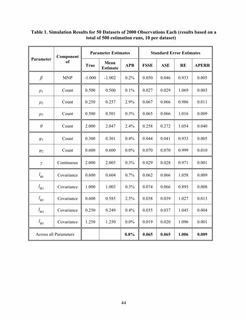
44

Table 1. Simulation Results for 50 Datasets of 2000 Observations Each (results based on a total of 500 estimation runs, 10 per dataset)

Parameter Component

of

Parameter Estimates Standard Error Estimates

True Mean

Estimate APB FSSE ASE RE APERR

β MNP -1.000 -1.002 0.2% 0.050 0.046 0.933 0.005

μ1 Count 0.500 0.500 0.1% 0.027 0.029 1.069 0.003

μ2 Count 0.250 0.257 2.9% 0.067 0.066 0.986 0.011

μ3 Count 0.500 0.501 0.3% 0.065 0.066 1.016 0.009

θ Count 2.000 2.047 2.4% 0.258 0.272 1.054 0.040

φ1 Count 0.300 0.301 0.4% 0.044 0.041 0.933 0.005

φ2 Count 0.600 0.600 0.0% 0.070 0.070 0.999 0.010

γ Continuous 2.000 2.005 0.3% 0.029 0.028 0.971 0.001

1Ωl Covariance 0.600 0.604 0.7% 0.062 0.066 1.058 0.009

2Ωl Covariance 1.000 1.003 0.3% 0.074 0.066 0.895 0.008

3Ωl Covariance 0.600 0.585 2.5% 0.038 0.039 1.027 0.013

4Ωl Covariance 0.250 0.249 0.4% 0.035 0.037 1.045 0.004

5Ωl Covariance 1.250 1.250 0.0% 0.019 0.020 1.096 0.001

Across all Parameters 0.8% 0.065 0.065 1.006 0.009

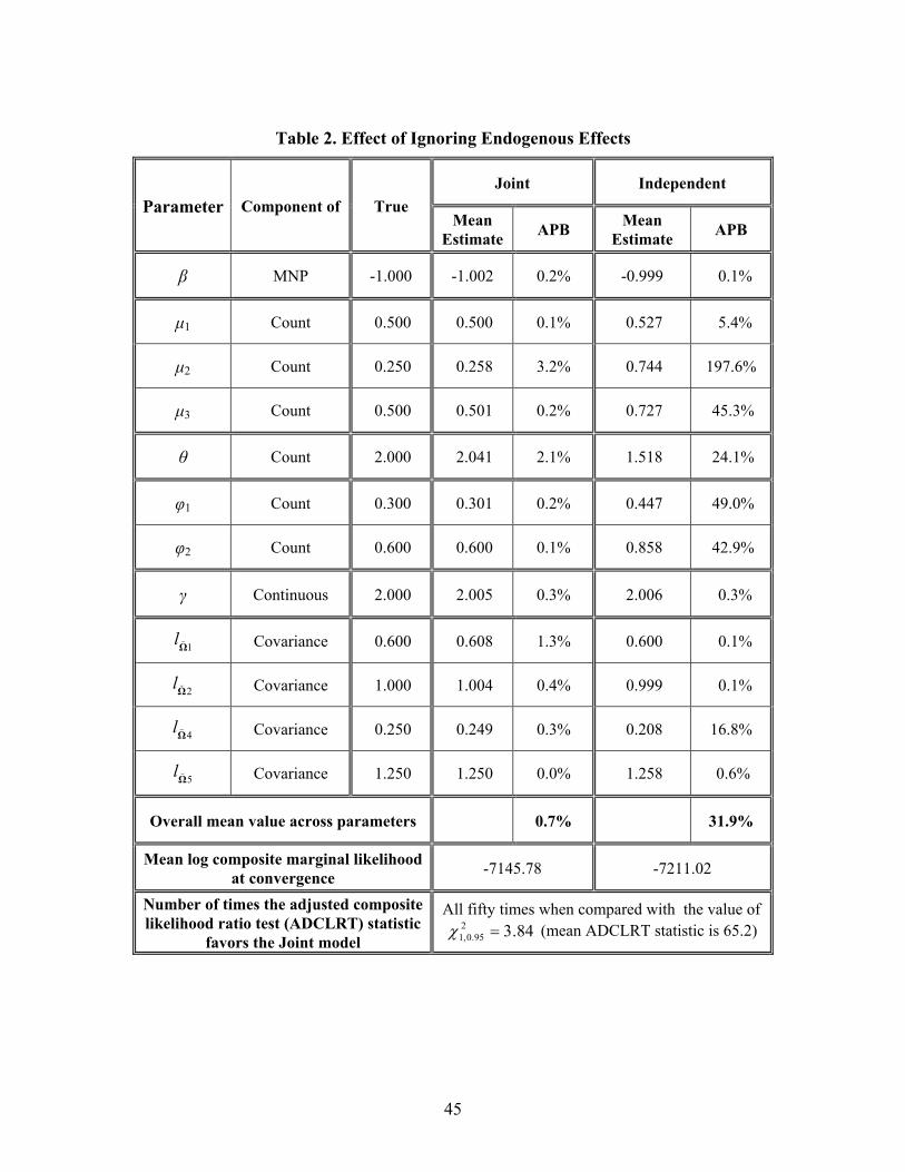
45

Table 2. Effect of Ignoring Endogenous Effects

Parameter Component of True

Joint Independent

Mean Estimate

APB Mean

Estimate APB

β MNP -1.000 -1.002 0.2% -0.999 0.1%

μ1 Count 0.500 0.500 0.1% 0.527 5.4%

μ2 Count 0.250 0.258 3.2% 0.744 197.6%

μ3 Count 0.500 0.501 0.2% 0.727 45.3%

θ Count 2.000 2.041 2.1% 1.518 24.1%

φ1 Count 0.300 0.301 0.2% 0.447 49.0%

φ2 Count 0.600 0.600 0.1% 0.858 42.9%

γ Continuous 2.000 2.005 0.3% 2.006 0.3%

1Ωl Covariance 0.600 0.608 1.3% 0.600 0.1%

2Ωl Covariance 1.000 1.004 0.4% 0.999 0.1%

4Ωl Covariance 0.250 0.249 0.3% 0.208 16.8%

5Ωl Covariance 1.250 1.250 0.0% 1.258 0.6%

Overall mean value across parameters 0.7% 31.9%

Mean log composite marginal likelihood at convergence

-7145.78 -7211.02

Number of times the adjusted composite likelihood ratio test (ADCLRT) statistic

favors the Joint model

All fifty times when compared with the value of 84.32

95.0,1 (mean ADCLRT statistic is 65.2)

46

Table 3. Sample Characteristics

Descriptive statistics

Dependent variables: MNP Variables

Location density [HHs per sq. mile] Number of observations (%)

0-99 108 (5.30)

100-499 262 (12.86)

500-1,999 619 (30.39)

≥ 2,000 1048 (51.42)

Dependent variables: Count Variables

Frequency

Motorized Vehicle Count

Number of motorized tours

Number of non-motorized tours

Number % Number % Number %

0 84 4.12 78 3.83 1359 66.72

1 516 25.33 539 26.46 415 20.37

2 917 45.02 532 26.12 154 7.56

3 357 17.53 346 16.99 59 2.90

4 108 5.30 208 10.21 35 1.72

5 38 1.87 116 5.69 9 0.44

6 9 0.44 87 4.27 4 0.20

7 4 0.20 48 2.36 1 0.05

8 2 0.10 32 1.57 1 0.05

9 1 0.05 22 1.08 0 0.00

10 or more 1 0.05 29 1.42 0 0.00

Dependent variables: Continuous Variable

Variable Mean Std. Dev. Min. Max. Natural logarithm of average tour distance

2.68 1.36 -2.30 5.60

47

Table 4. Model Estimation Result (variables significant at 5% level of significance unless otherwise noted)

Variables

MNP Counts LR

Density Categories [households per sq. mile] Number of

vehicles

Number of motorized

tours

Number of non-

motorized tours

Natural Log. of average tour

distance 0-99 100-499 500-1,999

≥2,000

Constant -1.341 -1.142 -0.756 - 0.251 0.470 -0.908 1.502

Family structure variables Single parent -0.961 - - - 0.167 0.587 0.703 Couple 0.202 0.202 - - 0.341 0.514 0.301 0.232 Nuclear family - - - - 0.363 1.065 1.116 Joint family - 0.260 - - 0.585 0.910 1.053 0.078††

Natural Log. of income [US$/year] 0.177 0.168 0.256 - 0.266 0.123 0.239

Household race and ethnicity variables Respondent race is Hispanic - - - - -0.094 -0.152†† Respondent race is Asian -0.193 -0.193 -0.193 - -0.254

Highest education status variable Highest education level is Bachelor’s degree or higher

-0.142† - - - -0.104 0.220

Immigrant variables All immigrants household -0.350 - - - 0.237† Combination of immigrant and non-immigrant household

-0.238† - - - 0.059†

Residential location (Density in housing units per square mile)

0-99 0.146 0.441 100-499 0.127 0.419 500-1,999 0.088 0.269

Number of vehicles 0.053 -0.163 0.235

Threshold parameters φ (flexibility parameter) 0.576 0.723 0.000* θ (dispersion parameter) 150.000* 150.000* 0.908

†Not significant at 5% level of significance but significant at 15% level of significance (15% level of significance corresponds to a t-statistic of 1.44). ††Not significant at the 15% level, but significant at the 30% level of significance (30% level of significance corresponds to a t-statistic of 1.04). * Fixed, because not statistically significantly different from value fixed to at even the 30% level

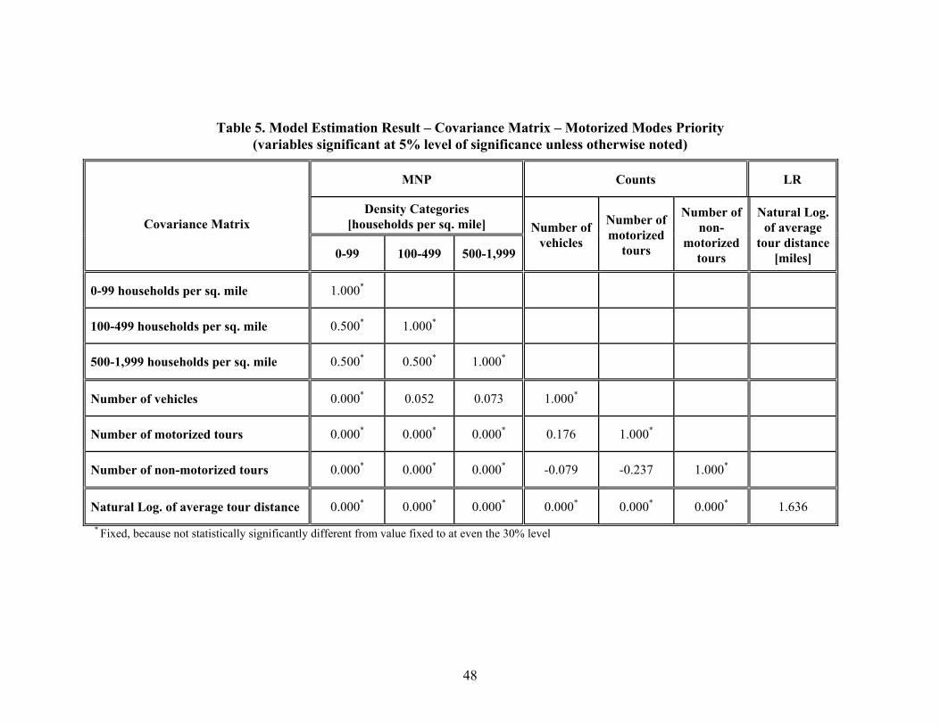
48

Table 5. Model Estimation Result – Covariance Matrix – Motorized Modes Priority (variables significant at 5% level of significance unless otherwise noted)

Covariance Matrix

MNP Counts LR

Density Categories [households per sq. mile] Number of

vehicles

Number of motorized

tours

Number of non-

motorized tours

Natural Log. of average

tour distance [miles] 0-99 100-499 500-1,999

0-99 households per sq. mile 1.000*

100-499 households per sq. mile 0.500* 1.000*

500-1,999 households per sq. mile 0.500* 0.500* 1.000*

Number of vehicles 0.000* 0.052 0.073 1.000*

Number of motorized tours 0.000* 0.000* 0.000* 0.176 1.000*

Number of non-motorized tours 0.000* 0.000* 0.000* -0.079 -0.237 1.000*

Natural Log. of average tour distance 0.000* 0.000* 0.000* 0.000* 0.000* 0.000* 1.636

* Fixed, because not statistically significantly different from value fixed to at even the 30% level

49

Table 6. Treatment Effects Corresponding to Transplanting a Random Household from a 500-1999 HHs per Sq. Mile Density Neighborhood to the Highest Density Neighborhood

Variable ATE from Joint

Model

ATE from Independent

Model

% Difference Attributable to

Self-Selection Effect (95% band)

“True” Effect (95% band)

Motorized vehicle ownership -0.189 -0.261 28

(10-46) 72

(54-90)

Number of motorized tours -0.038 -0.068 44

(26-62) 56

(38-74)

Number of non-motorized tours 0.016 0.027 41

(25-57) 59

(43-75)

Average tour distance -2.250 -3.083 27

(13-41) 73

(59-87)

Vehicle miles of travel -11.437 -15.960 28

(14-42) 72

(58-86)