A hybrid variable neighborhood search algorithm for solvingthe limited-buffer permutation flow shop scheduling problemwith the makespan criterion

Ghasem Moslehi n, Danial KhorasanianDepartment of Industrial and Systems Engineering, Isfahan University of Technology, Isfahan 84156-83111, Iran

a r t i c l e i n f o

Keywords:SchedulingLimited-buffer permutation flow shopMakespanVariable neighborhood searchSimulated annealing algorithmBlocking flow shop

a b s t r a c t

This paper investigates the limited-buffer permutation flow shop scheduling problem (LBPFSP) with themakespan criterion. A hybrid variable neighborhood search (HVNS) algorithm hybridized with thesimulated annealing algorithm is used to solve the problem. A method is also developed to decreasethe computational effort needed to implement different types of local search approaches used in theHVNS algorithm. Computational results show the higher efficiency of the HVNS algorithm as comparedwith the state-of-the-art algorithms. In addition, the HVNS algorithm is competitive with the algorithmsproposed in the literature for solving the blocking flow shop scheduling problem (i.e., LBPFSP with zero-capacity buffers), and finds 54 new upper bounds for the Taillard's benchmark instances.

& 2013 Elsevier Ltd. All rights reserved.

1. Introduction

The flow shop scheduling problem is one of the most popular casesof machine scheduling problems. Unlike the general assumptions ofthe problem, its intermediate buffers may have limited capacity dueto either technological considerations or process characteristics [1].The advents of just-in-time manufacturing and Kanban systems whichmaintain a limited in-process inventory have attracted the attention ofmost researchers to the limited-buffer permutation flow shop sche-duling problem (LBPFSP) [2]. In the case of LBPFSP with non-zerocapacity buffers, a completed job on a machine may block it until thenext intermediate buffer has a free space. Also, in the case with zerocapacity buffers, called the ‘blocking flow shop scheduling problem’

(BFSP), a completed job may block the machine until the nextdownstream machine is free. The process of no jobs can be startedon a machine, until a job blocks it. Hall and Sriskandarajah [1]presented a good review of the studies and applications of LBPFSPs.

In this paper, the LBPFSP with the makespan criterion isinvestigated. Papadimitriou and Kanellakis [3] proved the strongNP-hardness of the two-machine LBPFSP with a one-capacity bufferand the makespan criterion. Also, Hall and Sriskandarajah [1]showed that the three-machine BFSP with the makespan criterionis strongly NP-hard.

Due to the high complexity of the LBPFSP with the makespancriterion, attempts at its solution have invested more on the use ofheuristics than other methods. Leisten [4] compared some con-structive heuristics to arrive at the conclusion that the well-knownNawaz–Enscore–Ham (NEH) heuristic outperforms all others.Smutnicki [5] developed a tabu search (TS) algorithm for thetwo-machine case using H_block and S_block properties. The useof H_block and S_block properties may accelerate the local searchby initially eliminating the neighbors that do not improve thecurrent solution. Later, Nowicki [6] generalized Smutnicki's algo-rithm [5] to the m-machine case. Wang et al. [7] presented ahybrid genetic algorithm (HGA) and showed its superiority overthe TS algorithm. Further, Liu et al. [2] developed a hybrid particleswarm optimization (HPSO) algorithm which obtained bettersolutions for most benchmark instances than HGA did. Recently,Pan et al. [8] proposed a chaotic harmony search (CHS) algorithmand obtained better results compared to HGA or HPSO algorithms.Also, Qian [9] presented a hybrid differential evolution (HDE)algorithm for the multi-objective LBPFSP.

A greater number of approaches have been proposed for solvingthe BFSP with the makespan criterion than those developed forsolving the general case of the problem, i.e. the LBPFSP with themakespan criterion. Except for the branch and bound algorithmproposed by Ronconi [10] and that by Companys and Mateo [11],almost all other approaches are inexact. McCormick et al. [12]proposed a profile fitting (PF) heuristic. Later, Ronconi [13] presenteda minmax (MM) heuristic, a combination of NEH and MM (MME),and a combination of NEH and PF (PFE). Computational resultsshowed the superiority of MME and PFE over NEH. Caraffa et al. [14]

Contents lists available at ScienceDirect

journal homepage: www.elsevier.com/locate/caor

Computers & Operations Research

0305-0548/$ - see front matter & 2013 Elsevier Ltd. All rights reserved.http://dx.doi.org/10.1016/j.cor.2013.09.014

n Corresponding author. Tel.: þ98 311 391 5522; fax: þ98 31 139 15 526.E-mail addresses: moslehi@cc.iut.ac.ir, moslehi@istt.ir (G. Moslehi),

d.khorasanian@in.iut.ac.ir (D. Khorasanian).

Please cite this article as: Moslehi G, Khorasanian D. A hybrid variable neighborhood search algorithm for solving the limited-bufferpermutation flow shop scheduling problem.... Computers and Operations Research (2013), http://dx.doi.org/10.1016/j.cor.2013.09.014i

Computers & Operations Research ∎ (∎∎∎∎) ∎∎∎–∎∎∎

presented a genetic algorithm (GA) for this problem while Grabow-ski and Pempera [15] developed a TS algorithm and one with multi-moves (TSþM), both of which outperformed the GA. Wang et al.[16] developed a hybrid discrete differential evolution (HDDE)algorithm that outperformed the TS and TSþM proposed byGrabowski and Pempera [15]. Ribas et al. [17] presented an iteratedgreedy (IG) algorithm that outperformed the HDDE algorithm.Recently, Wang et al. [18] have proposed a hybrid modified global-best harmony search (hmgHS) algorithm which outperforms the IGalgorithm. For an initial solution generation, they used the NEH–Wang–Pan–Tasgetiren (NEH–WPT) heuristic which is a modifiedversion of the NEH and showed its superior performance over NEH.In another study, Wang et al. [19] developed a three-phase algorithm(TPA) which outperformed the IG algorithm with lower CPU-times.Finally, Lin and Ying [20] proposed a revised artificial immunesystem (RAIS) algorithm that outperformed the IG algorithm.No comparison has been made among the hmgHS, TPA, and RAISalgorithms in the past studies.

This paper aims to solve the LBPFSP with the makespancriterion using a variable neighborhood search (VNS) algorithmhybridized with the simulated annealing (SA) algorithm. The VNSalgorithm, a metaheuristic initially proposed by Mladenović andHansen [21], draws upon the idea of systematically changing theneighborhood structure. The algorithm and its variants have beensuccessfully used to solve some combinatorial optimization pro-blems [22–24], among others. According to this algorithm, first aninitial solution is generated. In a second stage, the three steps of‘shaking’, ‘local search’, and ‘neighborhood change’ are repeated inthis order until a stopping criterion is met. Algorithm 1 illustratesthese steps. In the shaking step, a neighbor x′ is generated for thecurrent solution (x) using the k-th pre-defined neighborhoodstructure (Nk) where kA{1, …, kmax}. In Line 6, Nk (x) representsa set including all neighbors of x generated by Nk. After the shakingstep, a local search is performed on x′. Finally, in the neighborhoodchange step, if the solution obtained from the local search step (x″)is better than x, it will be considered as the new current solution,and k will be equal to 1; otherwise, k¼kþ1. The hybrid VNSalgorithm (HVNS), presented in Section 4, uses the idea of the SAalgorithm in the local search step.

Algorithm 1. VNS algorithm

1 Generate an initial solution x;2 Repeat3 k¼1;4 Repeat5 %Shaking6 Generate a neighbor x′ANk (x);7 %Local search8 Obtain x″ by a local search for x′;9 %Neighborhood change10 If x″ is better than x11 x¼x″; k¼1;12 Else k¼kþ1;13 Endif14 Until k¼kmax

15 Until stopping criterion is met

The rest of the paper is organized as follows. Following thisIntroduction, the LBPFSP with the makespan criterion is formu-lated in Section 2. Section 3 provides the provisions needed forspeeding up the local search approaches. Section 4 developsthe HVNS algorithm for the problem. Algorithm settings and

computational results are presented in Section 5. Finally, conclu-sions and suggestions for future studies are presented in Section 6.

2. Problem formulation

In LBPFSP with the makespan criterion, there are n jobs thatshould be sequentially processed on a series of machines m1, m2,…,and mm. The operation Oi,r corresponds to the processing of job r,rA{1,…, n}, on machine i, {i¼1,…,m}, the processing time of whichis equal to pi,r. Between each two consecutive machines i and iþ1,i¼1, …, m�1, there exists a buffer with the size equal to BiZ0. Thejobs obey the first-in-first-out (FIFO) rule in the buffers, and thesequence in which the jobs are processed on each machine isconsequently identical. In the case with non-zero size buffers, acompleted job on a machine may block it until a free space isavailable in the intermediate buffer. Also, in BFSP, the completed jobon the machine may block it until the next downstream machine isfree. At any time, each machine can process at most one job, andeach job can be processed on at most one machine. The release timeof each job is equal to zero, and the set-up times are included in theprocessing times. Also, each job is processed without preemptionon each machine. The objective of the problem is to find a sequencethat minimizes the makespan.

Let us consider the sequence π¼(π (1), π (2), …, π (n)) whereπ (j) represents the j-th job in the sequence, further, define Si,j (π),i¼1, …, m, j¼1, …, n, as the earliest starting time of job π (j) onmachine i calculated from the following recursive formula [2]:

Si;jðπÞ ¼ maxðSi;j�1ðπÞþpi;πðj�1Þ; Si�1;jðπÞþpi�1;πðjÞ;

Siþ1;j�Bi �1ðπÞÞ; i¼ 1; :::;m; j¼ 1; :::;n ð1Þwhere, pi,π (j�1)¼0 and Si, j�1 (π)¼0 for j¼1, pi�1,π (j )¼0 and Si�1, j

(π)¼0 for i¼1, and Siþ1;j�Bi �1ðπÞ ¼ 0 for i¼m or jrBiþ1. Themakespan of the sequence π designated by Cmax (π) is equal to Sm,n

(π)þpm,π (n).

3. Preparations to speed up local search approaches

In LBPFSP, the precedence relationships existing between theoperations of jobs in a given sequence can be depicted in a directedgraph. In the graph for the sequence π¼(π (1), π (2), …, π(n)), thereare m�n nodes, where the node (i, j), iA{1, …, m}, jA{1, …, n}represents the operation Oi,π (j) and has a weight equal to pi, π (j).The graph has a horizontal arc between the nodes (i, j) and (i,jþ1),iA{1, …, m}, jA{1, …, n�1}, a vertical arc between the nodes (i, j)and (iþ1, j), iA{1, …, m�1}, jA{1, …, n}, and a skew arc betweenthe nodes (i, j) and (i�1, jþBi�1þ1), iA{2, …, m}, jA{1, …, n�Bi�1

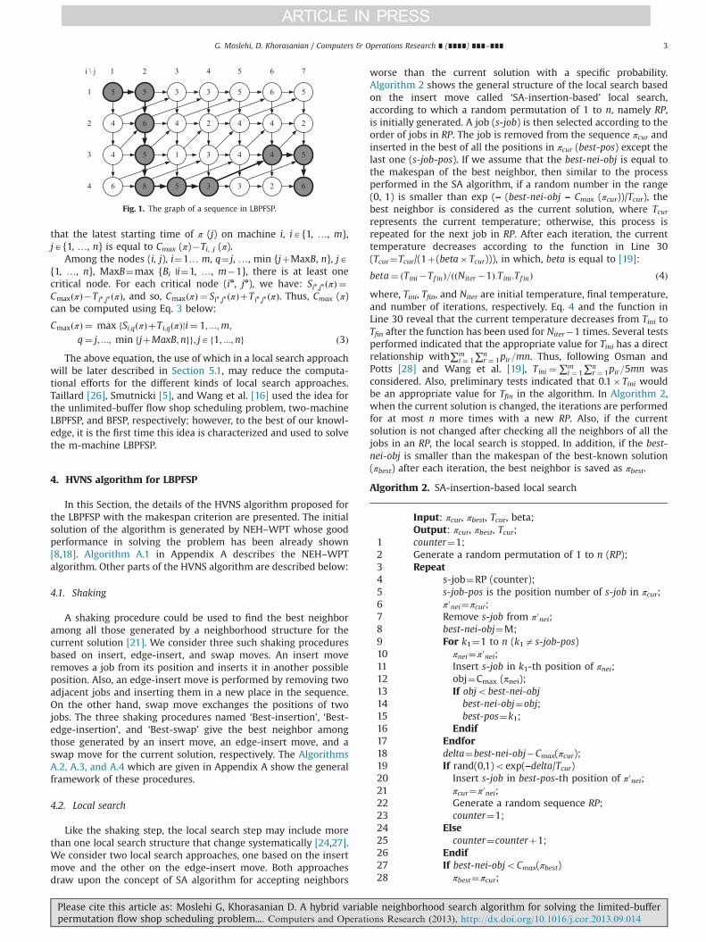
–1}. The skew arc between the nodes (i, j) and (i�1, jþBi�1þ1), iA{2, …, m}, jA{1, …, n�Bi�1–1} has a weight equal to (–pi, π(j)) whilethose of the other arcs are equal to zero. The length of the longestpath in the graph is equal to Cmax (π). The longest path, called the‘critical path’, contains some nodes with zero floating times, called‘critical nodes’. The values for the earliest and latest starting timesare the same for each critical node [25]. Fig. 1 shows the graph of asequence for a problem with n¼7, m¼4, B1¼B3¼1, and B2¼0. Theweight of each node is placed on it. Also, the critical nodes areshown in dark and bold typeface.

Define Ti,j (π), i A{1, …, m}, jA{1, …, n} as the duration betweenthe latest loading time of π (j) on machine i and Cmax (π), calculatedas follows based on the graph:

Ti;jðπÞ ¼ maxðTiþ1;jðπÞþpi;πðjÞ; Ti;jþ1ðπÞþpi;πðjÞ; Ti�1;jþBi� 1 þ1ðπÞÞ;i¼ 1; :::;m; j¼ 1; :::;n ð2Þ

where, Tiþ1;jðπÞ ¼ 0 for i¼m, Ti;jþ1ðπÞ ¼ 0 for j¼n, andTi�1;jþBi� 1 þ1ðπÞ ¼ 0 for i¼1 or j4n � Bi�1 1. It is straightforward

G. Moslehi, D. Khorasanian / Computers & Operations Research ∎ (∎∎∎∎) ∎∎∎–∎∎∎2

Please cite this article as: Moslehi G, Khorasanian D. A hybrid variable neighborhood search algorithm for solving the limited-bufferpermutation flow shop scheduling problem.... Computers and Operations Research (2013), http://dx.doi.org/10.1016/j.cor.2013.09.014i

that the latest starting time of π (j) on machine i, iA{1, …, m},jA{1, …, n} is equal to Cmax (π)�Ti, j (π).

Among the nodes (i, j), i¼1… m, q¼ j, …, min {jþMaxB, n}, jA{1, …, n}, MaxB¼max {Bi |i¼1, …, m�1}, there is at least onecritical node. For each critical node (in, jn), we have: Sin ;jn ðπÞ ¼CmaxðπÞ�Tin ;jn ðπÞ, and so, CmaxðπÞ ¼ Sin ;jn ðπÞþTin ;jn ðπÞ. Thus, Cmax (π)can be computed using Eq. 3 below:

CmaxðπÞ ¼ max fSi;qðπÞþTi;qðπÞji¼ 1; :::;m;

q¼ j; :::; min fjþMaxB;ngg; jAf1; :::;ng ð3ÞThe above equation, the use of which in a local search approach

will be later described in Section 5.1, may reduce the computa-tional efforts for the different kinds of local search approaches.Taillard [26], Smutnicki [5], and Wang et al. [16] used the idea forthe unlimited-buffer flow shop scheduling problem, two-machineLBPFSP, and BFSP, respectively; however, to the best of our knowl-edge, it is the first time this idea is characterized and used to solvethe m-machine LBPFSP.

4. HVNS algorithm for LBPFSP

In this Section, the details of the HVNS algorithm proposed forthe LBPFSP with the makespan criterion are presented. The initialsolution of the algorithm is generated by NEH–WPT whose goodperformance in solving the problem has been already shown[8,18]. Algorithm A.1 in Appendix A describes the NEH–WPTalgorithm. Other parts of the HVNS algorithm are described below:

4.1. Shaking

A shaking procedure could be used to find the best neighboramong all those generated by a neighborhood structure for thecurrent solution [21]. We consider three such shaking proceduresbased on insert, edge-insert, and swap moves. An insert moveremoves a job from its position and inserts it in another possibleposition. Also, an edge-insert move is performed by removing twoadjacent jobs and inserting them in a new place in the sequence.On the other hand, swap move exchanges the positions of twojobs. The three shaking procedures named ‘Best-insertion’, ‘Best-edge-insertion’, and ‘Best-swap’ give the best neighbor amongthose generated by an insert move, an edge-insert move, and aswap move for the current solution, respectively. The AlgorithmsA.2, A.3, and A.4 which are given in Appendix A show the generalframework of these procedures.

4.2. Local search

Like the shaking step, the local search step may include morethan one local search structure that change systematically [24,27].We consider two local search approaches, one based on the insertmove and the other on the edge-insert move. Both approachesdraw upon the concept of SA algorithm for accepting neighbors

worse than the current solution with a specific probability.Algorithm 2 shows the general structure of the local search basedon the insert move called ‘SA-insertion-based’ local search,according to which a random permutation of 1 to n, namely RP,is initially generated. A job (s-job) is then selected according to theorder of jobs in RP. The job is removed from the sequence πcur andinserted in the best of all the positions in πcur (best-pos) except thelast one (s-job-pos). If we assume that the best-nei-obj is equal tothe makespan of the best neighbor, then similar to the processperformed in the SA algorithm, if a random number in the range(0, 1) is smaller than exp (– (best-nei-obj – Cmax (πcur))/Tcur), thebest neighbor is considered as the current solution, where Tcurrepresents the current temperature; otherwise, this process isrepeated for the next job in RP. After each iteration, the currenttemperature decreases according to the function in Line 30(Tcur¼Tcur/(1þ(beta� Tcur))), in which, beta is equal to [19]:

beta¼ ðTini�Tf inÞ=ððNiter�1Þ:Tini:Tf inÞ ð4Þwhere, Tini, Tfin, and Niter are initial temperature, final temperature,and number of iterations, respectively. Eq. 4 and the function inLine 30 reveal that the current temperature decreases from Tini toTfin after the function has been used for Niter�1 times. Several testsperformed indicated that the appropriate value for Tini has a directrelationship with∑m

i ¼ 1∑nr ¼ 1pir=mn. Thus, following Osman and

Potts [28] and Wang et al. [19], Tini ¼∑mi ¼ 1∑

nr ¼ 1pir=5mn was

considered. Also, preliminary tests indicated that 0.1� Tini wouldbe an appropriate value for Tfin in the algorithm. In Algorithm 2,when the current solution is changed, the iterations are performedfor at most n more times with a new RP. Also, if the currentsolution is not changed after checking all the neighbors of all thejobs in an RP, the local search is stopped. In addition, if the best-nei-obj is smaller than the makespan of the best-known solution(πbest) after each iteration, the best neighbor is saved as πbest.

Algorithm 2. SA-insertion-based local search

Input: πcur, πbest, Tcur, beta;Output: πcur, πbest, Tcur;

1 counter¼1;2 Generate a random permutation of 1 to n (RP);3 Repeat4 s-job¼RP (counter);5 s-job-pos is the position number of s-job in πcur;6 π′nei¼πcur;7 Remove s-job from π′nei;8 best-nei-obj¼M;9 For k1¼1 to n (k1as-job-pos)10 πnei¼π′nei;11 Insert s-job in k1-th position of πnei;12 obj¼Cmax (πnei);13 If objobest-nei-obj14 best-nei-obj¼obj;15 best-pos¼k1;16 Endif17 Endfor18 delta¼best-nei-obj�Cmax(πcur);19 If rand(0,1)oexp(–delta/Tcur)20 Insert s-job in best-pos-th position of π′nei;21 πcur¼π′nei;22 Generate a random sequence RP;23 counter¼1;24 Else25 counter¼counterþ1;26 Endif27 If best-nei-objoCmax(πbest)28 πbest¼πcur;

Fig. 1. The graph of a sequence in LBPFSP.

G. Moslehi, D. Khorasanian / Computers & Operations Research ∎ (∎∎∎∎) ∎∎∎–∎∎∎ 3

Please cite this article as: Moslehi G, Khorasanian D. A hybrid variable neighborhood search algorithm for solving the limited-bufferpermutation flow shop scheduling problem.... Computers and Operations Research (2013), http://dx.doi.org/10.1016/j.cor.2013.09.014i

29 Endif30 Tcur¼Tcur/(1þ(beta� Tcur));31 Until counter4n;

The second local search approach, named ‘SA-edge-insertion-based’ local search, is similar to the previous one but with theedge-insert move instead of the insert move. The steps of this localsearch are illustrated in Algorithm A.5 given in Appendix A.

Algorithm 3 depicts the HVNS proposed in this paper. In thisalgorithm, the NEH–WPT heuristic is used to generate an initialsolution (πini), and both πcur and πbest are considered to be equal tothe thus obtained solution. In the shaking step, πcur is shaken bythe k-th (k¼1, …, kmax) shaking procedure (Nk (πcur)). Subse-quently, the first and second local searches, namely LC1 and LC2are performed in the local search step. In (πcur, πbest, Tcur)¼LCh (πcur,πbest, Tcur, beta), h¼1, 2 (Lines 14 and 16), (πcur, πbest, Tcur) and (πcur,πbest, Tcur, beta) are, respectively, the output and input data for LCh.The local search step is then repeated until the current solutionobtained from LC1 (i.e. πtemp) is changed after performing LC2.In the neighborhood change step, if the best solution of thepervious iteration has been improved, then we have k¼1; other-wise, k¼kþ1 is considered. Also, a time limit is considered as thestopping criterion.

Algorithm 3. HVNS algorithm

Input: Tini, Tfin, beta;Output: πbest;1 Generate an initial solution πini by NEH–WPT;2 πcur¼πini; πbest¼πini; pervious-best-obj¼Cmax (πini);3 Repeat4 k¼1;5 Repeat6 %Shaking7 Generate a neighbor πcur¼Nk (πcur);8 If Cmax (πcur)oCmax (πbest)9 πbest¼πcur;10 Endif11 %local search12 tag¼0;13 Repeat14 (πcur, πbest, Tcur)¼LC1 (πcur, πbest, Tcur, beta);15 πtemp¼πcur;16 (πcur, πbest, Tcur)¼LC2 (πcur, πbest, Tcur, beta);17 If πtemp¼πcur18 tag¼1;19 Endif20 Until tag¼121 %Neighborhood change22 If Cmax (πbest)opervious-best-obj23 k¼1;24 pervious-best-obj¼Cmax (πbest);25 Else k¼kþ1;26 Endif27 Until k¼kmax

28 Until time-limit is met

5. Computational experiments

In this Section, the HVNS algorithm is adjusted and its resultsare compared with those of the best algorithms previouslyproposed for the problem considering a same time limit. Similarto almost all the approaches proposed earlier for solving LBPFSP,

the computational simulations were carried out using 31 bench-mark instances including Car1–Car8 [29], Hel1–Hel2 [30], andRec01–Rec41 [31], with buffer sizes (B) equal to 0, 2, and 4. Theseare named Carlier–Heller–Reeves (CHR) instances. The processingtimes of Car1–Car8, Hel1–Hel2, and Rec01–Rec41 are chosen fromthe uniform distributions [1,999], [1,9], and [1,99], respectively.However, Taillard's benchmark instances [32] have been producedfor the permutation flow shop scheduling problem originally, thecomputational experiments of the algorithms performed for BFSPhave often been based on these instances. Therefore, the perfor-mance of the HVNS algorithm for the BFSP (i.e., LBPFSP with B¼0)was also evaluated on Taillard's instances composed of 120instances in 12 groups with the size ranging from 20 jobs and5 machines to 500 jobs and 20 machines. All the evaluations wereperformed on a pc with Intel Core2 Duo T9600 CPU, 2.8 GHz and4 GB RAM. To analyze the effectiveness of solution A for aninstance, the relative percentage deviation (RPD) calculated bythe following equation was used:

RPDðAÞ ¼ CmaxðAÞ�bestobjbestobj

� 100 ð5Þ

where, “bestobj” represents the best-known makespan for theinstance.

5.1. Speed up method for local search approaches

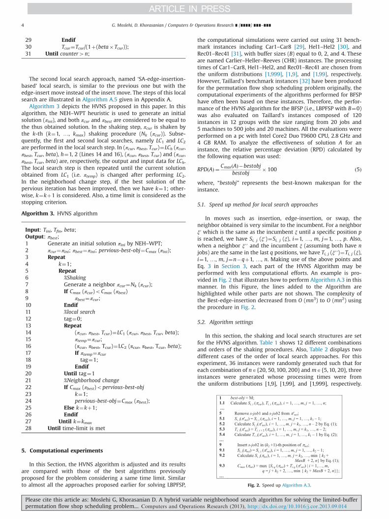
In moves such as insertion, edge-insertion, or swap, theneighbor obtained is very similar to the incumbent. For a neighborξ′ which is the same as the incumbent ξ until a specific position pis reached, we have Si, j (ξ′)¼Si, j (ξ), i¼1, …, m, j¼1, …, p. Also,when a neighbor ξ′′ and the incumbent ξ (assuming both have njobs) are the same in the last q positions, we have Ti, j (ξ′′)¼Ti, j (ξ),i¼1, …, m, j¼n�qþ1, …, n. Making use of the above points andEq. 3 in Section 3, each part of the HVNS Algorithm may beperformed with less computational efforts. An example is pro-vided in Fig. 2 that illustrates how to perform Algorithm A.3 in thismanner. In this Figure, the lines added to the Algorithm arehighlighted while other parts are not shown. The complexity ofthe Best-edge-insertion decreased from O (mn3) to O (mn2) usingthe procedure in Fig. 2.

5.2. Algorithm settings

In this section, the shaking and local search structures are setfor the HVNS algorithm. Table 1 shows 12 different combinationsand orders of the shaking procedures. Also, Table 2 displays twodifferent cases of the order of local search approaches. For thisexperiment, 36 instances were randomly generated such that foreach combination of nA{20, 50, 100, 200} andmA{5, 10, 20}, threeinstances were generated whose processing times were fromthe uniform distributions [1,9], [1,99], and [1,999], respectively.

Fig. 2. Speed up Algorithm A.3.

G. Moslehi, D. Khorasanian / Computers & Operations Research ∎ (∎∎∎∎) ∎∎∎–∎∎∎4

Please cite this article as: Moslehi G, Khorasanian D. A hybrid variable neighborhood search algorithm for solving the limited-bufferpermutation flow shop scheduling problem.... Computers and Operations Research (2013), http://dx.doi.org/10.1016/j.cor.2013.09.014i

For each instance, three buffer sizes were considered that includedall buffer sizes equal to zero (B¼0), two (B¼2), and four (B¼4),respectively. This yielded a total number of 108 instances in theexperiment.

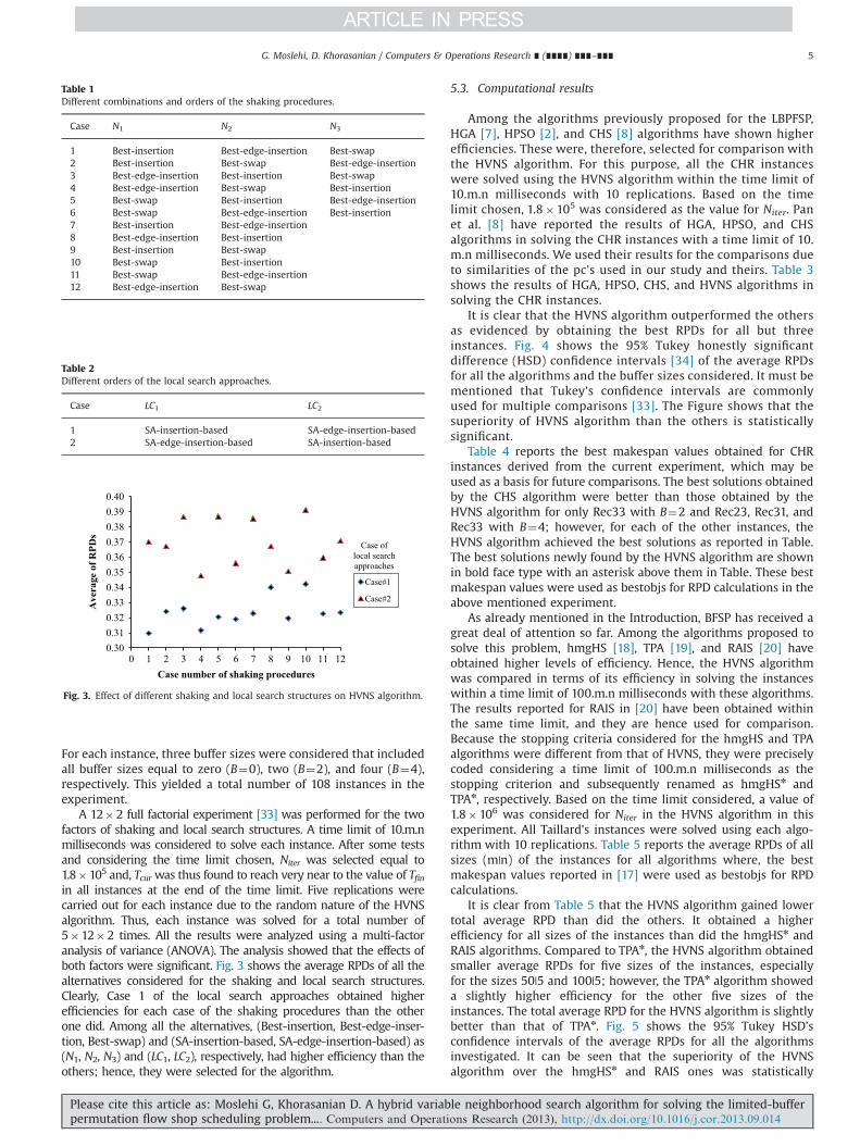
A 12�2 full factorial experiment [33] was performed for the twofactors of shaking and local search structures. A time limit of 10.m.nmilliseconds was considered to solve each instance. After some testsand considering the time limit chosen, Niter was selected equal to1.8�105 and, Tcur was thus found to reach very near to the value of Tfinin all instances at the end of the time limit. Five replications werecarried out for each instance due to the random nature of the HVNSalgorithm. Thus, each instance was solved for a total number of5�12�2 times. All the results were analyzed using a multi-factoranalysis of variance (ANOVA). The analysis showed that the effects ofboth factors were significant. Fig. 3 shows the average RPDs of all thealternatives considered for the shaking and local search structures.Clearly, Case 1 of the local search approaches obtained higherefficiencies for each case of the shaking procedures than the otherone did. Among all the alternatives, (Best-insertion, Best-edge-inser-tion, Best-swap) and (SA-insertion-based, SA-edge-insertion-based) as(N1, N2, N3) and (LC1, LC2), respectively, had higher efficiency than theothers; hence, they were selected for the algorithm.

5.3. Computational results

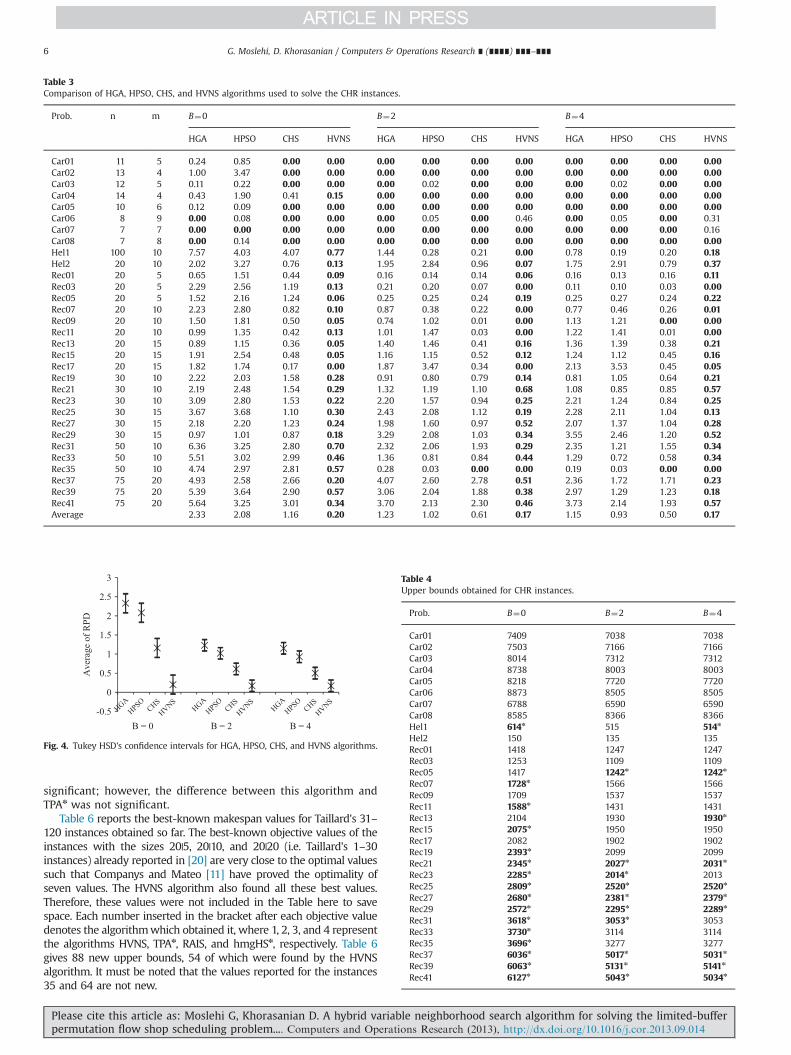
Among the algorithms previously proposed for the LBPFSP,HGA [7], HPSO [2], and CHS [8] algorithms have shown higherefficiencies. These were, therefore, selected for comparison withthe HVNS algorithm. For this purpose, all the CHR instanceswere solved using the HVNS algorithm within the time limit of10.m.n milliseconds with 10 replications. Based on the timelimit chosen, 1.8�105 was considered as the value for Niter. Panet al. [8] have reported the results of HGA, HPSO, and CHSalgorithms in solving the CHR instances with a time limit of 10.m.n milliseconds. We used their results for the comparisons dueto similarities of the pc's used in our study and theirs. Table 3shows the results of HGA, HPSO, CHS, and HVNS algorithms insolving the CHR instances.

It is clear that the HVNS algorithm outperformed the othersas evidenced by obtaining the best RPDs for all but threeinstances. Fig. 4 shows the 95% Tukey honestly significantdifference (HSD) confidence intervals [34] of the average RPDsfor all the algorithms and the buffer sizes considered. It must bementioned that Tukey's confidence intervals are commonlyused for multiple comparisons [33]. The Figure shows that thesuperiority of HVNS algorithm than the others is statisticallysignificant.

Table 4 reports the best makespan values obtained for CHRinstances derived from the current experiment, which may beused as a basis for future comparisons. The best solutions obtainedby the CHS algorithm were better than those obtained by theHVNS algorithm for only Rec33 with B¼2 and Rec23, Rec31, andRec33 with B¼4; however, for each of the other instances, theHVNS algorithm achieved the best solutions as reported in Table.The best solutions newly found by the HVNS algorithm are shownin bold face type with an asterisk above them in Table. These bestmakespan values were used as bestobjs for RPD calculations in theabove mentioned experiment.

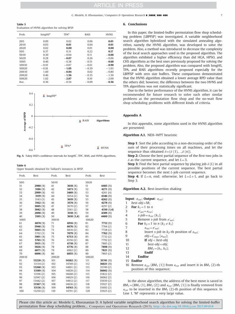
As already mentioned in the Introduction, BFSP has received agreat deal of attention so far. Among the algorithms proposed tosolve this problem, hmgHS [18], TPA [19], and RAIS [20] haveobtained higher levels of efficiency. Hence, the HVNS algorithmwas compared in terms of its efficiency in solving the instanceswithin a time limit of 100.m.n milliseconds with these algorithms.The results reported for RAIS in [20] have been obtained withinthe same time limit, and they are hence used for comparison.Because the stopping criteria considered for the hmgHS and TPAalgorithms were different from that of HVNS, they were preciselycoded considering a time limit of 100.m.n milliseconds as thestopping criterion and subsequently renamed as hmgHSn andTPAn, respectively. Based on the time limit considered, a value of1.8�106 was considered for Niter in the HVNS algorithm in thisexperiment. All Taillard's instances were solved using each algo-rithm with 10 replications. Table 5 reports the average RPDs of allsizes (m|n) of the instances for all algorithms where, the bestmakespan values reported in [17] were used as bestobjs for RPDcalculations.

It is clear from Table 5 that the HVNS algorithm gained lowertotal average RPD than did the others. It obtained a higherefficiency for all sizes of the instances than did the hmgHSn andRAIS algorithms. Compared to TPAn, the HVNS algorithm obtainedsmaller average RPDs for five sizes of the instances, especiallyfor the sizes 50|5 and 100|5; however, the TPAn algorithm showeda slightly higher efficiency for the other five sizes of theinstances. The total average RPD for the HVNS algorithm is slightlybetter than that of TPAn. Fig. 5 shows the 95% Tukey HSD’sconfidence intervals of the average RPDs for all the algorithmsinvestigated. It can be seen that the superiority of the HVNSalgorithm over the hmgHSn and RAIS ones was statistically

Table 1Different combinations and orders of the shaking procedures.

Case N1 N2 N3

1 Best-insertion Best-edge-insertion Best-swap2 Best-insertion Best-swap Best-edge-insertion3 Best-edge-insertion Best-insertion Best-swap4 Best-edge-insertion Best-swap Best-insertion5 Best-swap Best-insertion Best-edge-insertion6 Best-swap Best-edge-insertion Best-insertion7 Best-insertion Best-edge-insertion8 Best-edge-insertion Best-insertion9 Best-insertion Best-swap10 Best-swap Best-insertion11 Best-swap Best-edge-insertion12 Best-edge-insertion Best-swap

Table 2Different orders of the local search approaches.

Case LC1 LC2

1 SA-insertion-based SA-edge-insertion-based2 SA-edge-insertion-based SA-insertion-based

0.300.310.320.330.340.350.360.370.380.390.40

0 1 2 3 4 5 6 7 8 9 10 11 12

Ave

rage

of R

PDs

Case number of shaking procedures

Case#1

Case#2

Case of local search approaches

Fig. 3. Effect of different shaking and local search structures on HVNS algorithm.

G. Moslehi, D. Khorasanian / Computers & Operations Research ∎ (∎∎∎∎) ∎∎∎–∎∎∎ 5

Please cite this article as: Moslehi G, Khorasanian D. A hybrid variable neighborhood search algorithm for solving the limited-bufferpermutation flow shop scheduling problem.... Computers and Operations Research (2013), http://dx.doi.org/10.1016/j.cor.2013.09.014i

significant; however, the difference between this algorithm andTPAn was not significant.

Table 6 reports the best-known makespan values for Taillard's 31–120 instances obtained so far. The best-known objective values of theinstances with the sizes 20|5, 20|10, and 20|20 (i.e. Taillard's 1–30instances) already reported in [20] are very close to the optimal valuessuch that Companys and Mateo [11] have proved the optimality ofseven values. The HVNS algorithm also found all these best values.Therefore, these values were not included in the Table here to savespace. Each number inserted in the bracket after each objective valuedenotes the algorithmwhich obtained it, where 1, 2, 3, and 4 representthe algorithms HVNS, TPAn, RAIS, and hmgHSn, respectively. Table 6gives 88 new upper bounds, 54 of which were found by the HVNSalgorithm. It must be noted that the values reported for the instances35 and 64 are not new.

Table 3Comparison of HGA, HPSO, CHS, and HVNS algorithms used to solve the CHR instances.

Prob. n m B¼0 B¼2 B¼4

HGA HPSO CHS HVNS HGA HPSO CHS HVNS HGA HPSO CHS HVNS

Car01 11 5 0.24 0.85 0.00 0.00 0.00 0.00 0.00 0.00 0.00 0.00 0.00 0.00Car02 13 4 1.00 3.47 0.00 0.00 0.00 0.00 0.00 0.00 0.00 0.00 0.00 0.00Car03 12 5 0.11 0.22 0.00 0.00 0.00 0.02 0.00 0.00 0.00 0.02 0.00 0.00Car04 14 4 0.43 1.90 0.41 0.15 0.00 0.00 0.00 0.00 0.00 0.00 0.00 0.00Car05 10 6 0.12 0.09 0.00 0.00 0.00 0.00 0.00 0.00 0.00 0.00 0.00 0.00Car06 8 9 0.00 0.08 0.00 0.00 0.00 0.05 0.00 0.46 0.00 0.05 0.00 0.31Car07 7 7 0.00 0.00 0.00 0.00 0.00 0.00 0.00 0.00 0.00 0.00 0.00 0.16Car08 7 8 0.00 0.14 0.00 0.00 0.00 0.00 0.00 0.00 0.00 0.00 0.00 0.00Hel1 100 10 7.57 4.03 4.07 0.77 1.44 0.28 0.21 0.00 0.78 0.19 0.20 0.18Hel2 20 10 2.02 3.27 0.76 0.13 1.95 2.84 0.96 0.07 1.75 2.91 0.79 0.37Rec01 20 5 0.65 1.51 0.44 0.09 0.16 0.14 0.14 0.06 0.16 0.13 0.16 0.11Rec03 20 5 2.29 2.56 1.19 0.13 0.21 0.20 0.07 0.00 0.11 0.10 0.03 0.00Rec05 20 5 1.52 2.16 1.24 0.06 0.25 0.25 0.24 0.19 0.25 0.27 0.24 0.22Rec07 20 10 2.23 2.80 0.82 0.10 0.87 0.38 0.22 0.00 0.77 0.46 0.26 0.01Rec09 20 10 1.50 1.81 0.50 0.05 0.74 1.02 0.01 0.00 1.13 1.21 0.00 0.00Rec11 20 10 0.99 1.35 0.42 0.13 1.01 1.47 0.03 0.00 1.22 1.41 0.01 0.00Rec13 20 15 0.89 1.15 0.36 0.05 1.40 1.46 0.41 0.16 1.36 1.39 0.38 0.21Rec15 20 15 1.91 2.54 0.48 0.05 1.16 1.15 0.52 0.12 1.24 1.12 0.45 0.16Rec17 20 15 1.82 1.74 0.17 0.00 1.87 3.47 0.34 0.00 2.13 3.53 0.45 0.05Rec19 30 10 2.22 2.03 1.58 0.28 0.91 0.80 0.79 0.14 0.81 1.05 0.64 0.21Rec21 30 10 2.19 2.48 1.54 0.29 1.32 1.19 1.10 0.68 1.08 0.85 0.85 0.57Rec23 30 10 3.09 2.80 1.53 0.22 2.20 1.57 0.94 0.25 2.21 1.24 0.84 0.25Rec25 30 15 3.67 3.68 1.10 0.30 2.43 2.08 1.12 0.19 2.28 2.11 1.04 0.13Rec27 30 15 2.18 2.20 1.23 0.24 1.98 1.60 0.97 0.52 2.07 1.37 1.04 0.28Rec29 30 15 0.97 1.01 0.87 0.18 3.29 2.08 1.03 0.34 3.55 2.46 1.20 0.52Rec31 50 10 6.36 3.25 2.80 0.70 2.32 2.06 1.93 0.29 2.35 1.21 1.55 0.34Rec33 50 10 5.51 3.02 2.99 0.46 1.36 0.81 0.84 0.44 1.29 0.72 0.58 0.34Rec35 50 10 4.74 2.97 2.81 0.57 0.28 0.03 0.00 0.00 0.19 0.03 0.00 0.00Rec37 75 20 4.93 2.58 2.66 0.20 4.07 2.60 2.78 0.51 2.36 1.72 1.71 0.23Rec39 75 20 5.39 3.64 2.90 0.57 3.06 2.04 1.88 0.38 2.97 1.29 1.23 0.18Rec41 75 20 5.64 3.25 3.01 0.34 3.70 2.13 2.30 0.46 3.73 2.14 1.93 0.57Average 2.33 2.08 1.16 0.20 1.23 1.02 0.61 0.17 1.15 0.93 0.50 0.17

-0.5

0

0.5

1

1.5

2

2.5

3

Ave

rage

of R

PD

B = 0 B = 2 B = 4

Fig. 4. Tukey HSD's confidence intervals for HGA, HPSO, CHS, and HVNS algorithms.

Table 4Upper bounds obtained for CHR instances.

Prob. B¼0 B¼2 B¼4

Car01 7409 7038 7038Car02 7503 7166 7166Car03 8014 7312 7312Car04 8738 8003 8003Car05 8218 7720 7720Car06 8873 8505 8505Car07 6788 6590 6590Car08 8585 8366 8366Hel1 614n 515 514n

Hel2 150 135 135Rec01 1418 1247 1247Rec03 1253 1109 1109Rec05 1417 1242n 1242n

Rec07 1728n 1566 1566Rec09 1709 1537 1537Rec11 1588n 1431 1431Rec13 2104 1930 1930n

Rec15 2075n 1950 1950Rec17 2082 1902 1902Rec19 2393n 2099 2099Rec21 2345n 2027n 2031n

Rec23 2285n 2014n 2013Rec25 2809n 2520n 2520n

Rec27 2680n 2381n 2379n

Rec29 2572n 2295n 2289n

Rec31 3618n 3053n 3053Rec33 3730n 3114 3114Rec35 3696n 3277 3277Rec37 6036n 5017n 5031n

Rec39 6063n 5131n 5141n

Rec41 6127n 5043n 5034n

G. Moslehi, D. Khorasanian / Computers & Operations Research ∎ (∎∎∎∎) ∎∎∎–∎∎∎6

Please cite this article as: Moslehi G, Khorasanian D. A hybrid variable neighborhood search algorithm for solving the limited-bufferpermutation flow shop scheduling problem.... Computers and Operations Research (2013), http://dx.doi.org/10.1016/j.cor.2013.09.014i

6. Conclusions

In this paper, the limited-buffer permutation flow shop schedul-ing problem (LBPFSP) was investigated. A variable neighborhoodsearch algorithm hybridized with the simulated annealing algo-rithm, namely the HVNS algorithm, was developed to solve theproblem. Also, a method was introduced to decrease the complexityof the local search approaches used in the proposed algorithm. Thealgorithm exhibited a higher efficiency than did HGA, HPSO, andCHS algorithms as the best ones previously proposed for solving theproblem. Also, the proposed algorithm was compared with hmgHS,TPA, and RAIS algorithms recently proposed especially for theLBPFSP with zero size buffers. These comparisons demonstratedthat the HVNS algorithm obtained a lower average RPD value thanthe others did; however, the difference between the two HVNS andTPA algorithms was not statistically significant.

Due to the better performance of the HVNS algorithm, it can berecommended for future research to solve such other similarproblems as the permutation flow shop and the no-wait flowshop scheduling problems with different kinds of criteria.

Appendix A

In this appendix, some algorithms used in the HVNS algorithmare presented:

Algorithm A.1. NEH–WPT heuristic

Step 1: Sort the jobs according to a non-decreasing order of thesum of their processing times on all machines, and let thesequence thus obtained δ¼(δ (1),…,δ (n)).Step 2: Choose the best partial sequence of the first two jobs inδ as the current sequence, and let L¼3.Step 3: Find the best partial sequence by placing job δ (L) in allpossible positions of the current sequence. The best partialsequence becomes the next L-job current sequence.Step 4: If L¼n, end; otherwise, let L¼Lþ1, and go back toStep 3.

Algorithm A.2. Best-insertion shaking

Input: πcur; Output: πcur;1 best-obj¼M;2 For k1¼1 to n3 π'nei¼πcur;4 s-job¼πcur (k1);5 Remove s-job from π'nei;6 For k2¼1 to n (k2ak1)7 πnei¼π'nei;8 Insert s-job in k2-th position of πnei;9 obj¼Cmax (πnei);10 If objobest-obj11 best-obj¼obj;12 BM1¼(k1, k2);13 Endif14 Endfor15 Endfor16 Remove πcur (BM1 (1)) from πcur and insert it in BM1 (2)-th

position of this sequence;

In the above algorithm, the address of the best move is saved inBM1¼(BM1 (1), BM1 (2)) and πcur (BM1 (1)) is finally removed fromπcur to be inserted in the BM1 (2)-th position of this sequence. InLine 1, ‘M’ represents a very large value.

Table 5Evaluation of HVNS algorithm for solving BFSP.

Prob. hmgHSn TPAn RAIS HVNS

20|5 0.09 0.02 0.06 0.0120|10 0.03 0.01 0.04 0.0120|20 0.02 0.00 0.01 0.0050|5 0.37 0.31 0.22 0.1750|10 0.30 �0.04 0.11 �0.0650|20 0.28 �0.07 0.26 �0.06100|5 0.40 �0.38 �0.51 �0.60100|10 �0.10 �0.87 �0.61 �0.90100|20 �0.18 �1.05 �0.39 �1.03200|10 1.60 �0.84 0.02 �0.80200|20 0.46 �1.56 �0.35 �1.50500|20 1.02 �2.07 0.10 �2.00Ave. 0.36 �0.54 �0.09 �0.56

hmgHS*

HVNSTPA*

RAIS

-0.6

-0.4

-0.2

0

0.2

0.4

Ave

rage

of R

PD

Algorithms

Fig. 5. Tukey HSD's confidence intervals for hmgHS*, TPA*, RAIS, and HVNS algorithms.

Table 6Upper bounds obtained for Taillard's instances in BFSP.

Prob. Best Prob. Best Prob. Best

50|5 50|10 50|2031 2980 (1) 41 3618 (1) 51 4485 (1)32 3186 (1) 42 3473 (1) 52 4271 (1)33 2999 (1) 43 3469 (1) 53 4261 (4)34 3119 (1) 44 3654 (2) 54 4346 (1)35 3143 (3) 45 3619 (1) 55 4262 (1)36 3162 (1) 46 3574 (1) 56 4278 (1)37 3005 (1) 47 3670 (2) 57 4297 (2)38 3042 (1) 48 3561 (2) 58 4310 (1,4)39 2898 (1) 49 3518 (1) 59 4309 (1)40 3105 (1) 50 3610 (1,4) 60 4400 (1)100|5 100|10 100|2061 6074 (1) 71 6916 (1) 81 7712 (1)62 5946 (1) 72 6676 (1) 82 7764 (2)63 5865 (1) 73 6816 (2) 83 7728 (2)64 5702 (3) 74 7079 (1) 84 7762 (1)65 5901 (1) 75 6753 (1) 85 7732 (2)66 5765 (1) 76 6556 (2) 86 7792 (2)67 5931 (1) 77 6718 (1) 87 7885 (2)68 5826 (1) 78 6776 (1) 88 7898 (1)69 6071 (1) 79 6962 (2) 89 7821 (1)70 6096 (1) 80 6855 (1) 90 7865 (2)200|10 200|20 500|2091 13228 (1) 101 14582 (1) 111 35741 (1)92 13134 (2) 102 14749 (2) 112 36021 (1)93 13260 (1) 103 14891 (2) 113 35749 (2)94 13189 (1) 104 14820 (2) 114 36002 (1)95 13196 (2) 105 14668 (2) 115 35822 (2)96 12947 (2) 106 14829 (2) 116 36062 (2)97 13442 (2) 107 14812 (2) 117 35650 (2)98 13367 (1) 108 14836 (2) 118 35927 (2)99 13136 (1) 109 14743 (1) 119 35692 (2)100 13250 (2) 110 14791 (2) 120 35925 (2)

G. Moslehi, D. Khorasanian / Computers & Operations Research ∎ (∎∎∎∎) ∎∎∎–∎∎∎ 7

Please cite this article as: Moslehi G, Khorasanian D. A hybrid variable neighborhood search algorithm for solving the limited-bufferpermutation flow shop scheduling problem.... Computers and Operations Research (2013), http://dx.doi.org/10.1016/j.cor.2013.09.014i

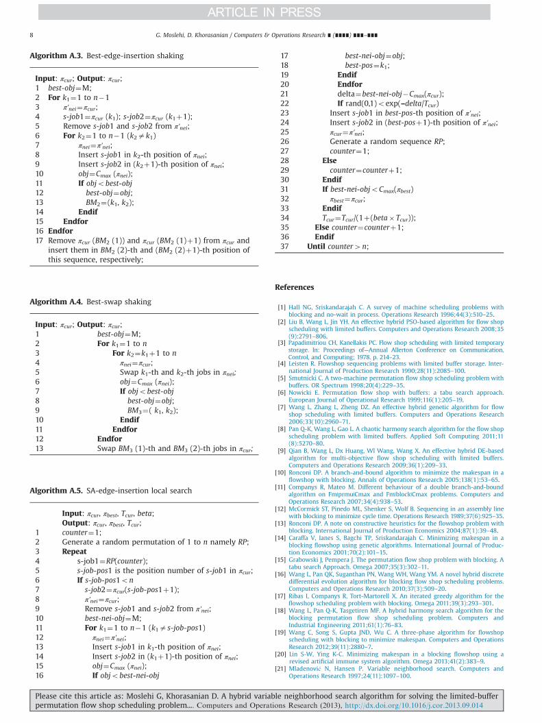
Algorithm A.3. Best-edge-insertion shaking

Input: πcur; Output: πcur;1 best-obj¼M;2 For k1¼1 to n�13 π'nei¼πcur;4 s-job1¼πcur (k1); s-job2¼πcur (k1þ1);5 Remove s-job1 and s-job2 from π'nei;6 For k2¼1 to n�1 (k2ak1)7 πnei¼π'nei;8 Insert s-job1 in k2-th position of πnei;9 Insert s-job2 in (k2þ1)-th position of πnei;10 obj¼Cmax (πnei);11 If objobest-obj12 best-obj¼obj;13 BM2¼(k1, k2);14 Endif15 Endfor16 Endfor17 Remove πcur (BM2 (1)) and πcur (BM2 (1)þ1) from πcur and

insert them in BM2 (2)-th and (BM2 (2)þ1)-th position ofthis sequence, respectively;

Algorithm A.4. Best-swap shaking

Input: πcur; Output: πcur;1 best-obj¼M;2 For k1¼1 to n3 For k2¼k1þ1 to n4 πnei¼πcur;5 Swap k1-th and k2-th jobs in πnei;6 obj¼Cmax (πnei);7 If objobest-obj8 best-obj¼obj;9 BM3¼( k1, k2);10 Endif11 Endfor12 Endfor13 Swap BM3 (1)-th and BM3 (2)-th jobs in πcur;

Algorithm A.5. SA-edge-insertion local search

Input: πcur, πbest, Tcur, beta;Output: πcur, πbest, Tcur;

1 counter¼1;2 Generate a random permutation of 1 to n namely RP;3 Repeat4 s-job1¼RP(counter);5 s-job-pos1 is the position number of s-job1 in πcur;6 If s-job-pos1on7 s-job2¼πcur(s-job-pos1þ1);8 π'nei¼πcur;9 Remove s-job1 and s-job2 from π'nei;10 best-nei-obj¼M;11 For k1¼1 to n�1 (k1as-job-pos1)12 πnei¼π'nei;13 Insert s-job1 in k1-th position of πnei;14 Insert s-job2 in (k1þ1)-th position of πnei;15 obj¼Cmax (πnei);16 If objobest-nei-obj

17 best-nei-obj¼obj;18 best-pos¼k1;19 Endif20 Endfor21 delta¼best-nei-obj�Cmax(πcur);22 If rand(0,1)oexp(–delta/Tcur)23 Insert s-job1 in best-pos-th position of π'nei;24 Insert s-job2 in (best-posþ1)-th position of π'nei;25 πcur¼π'nei;26 Generate a random sequence RP;27 counter¼1;28 Else29 counter¼counterþ1;30 Endif31 If best-nei-objoCmax(πbest)32 πbest¼πcur;33 Endif34 Tcur¼Tcur/(1þ(beta� Tcur));35 Else counter¼counterþ1;36 Endif37 Until counter4n;

References

[1] Hall NG, Sriskandarajah C. A survey of machine scheduling problems withblocking and no-wait in process. Operations Research 1996;44(3):510–25.

[2] Liu B, Wang L, Jin YH. An effective hybrid PSO-based algorithm for flow shopscheduling with limited buffers. Computers and Operations Research 2008;35(9):2791–806.

[3] Papadimitriou CH, Kanellakis PC. Flow shop scheduling with limited temporarystorage. In: Proceedings of—Annual Allerton Conference on Communication,Control, and Computing; 1978. p. 214–23.

[4] Leisten R. Flowshop sequencing problems with limited buffer storage. Inter-national Journal of Production Research 1990;28(11):2085–100.

[5] Smutnicki C. A two-machine permutation flow shop scheduling problem withbuffers. OR Spectrum 1998;20(4):229–35.

[6] Nowicki E. Permutation flow shop with buffers: a tabu search approach.European Journal of Operational Research 1999;116(1):205–19.

[7] Wang L, Zhang L, Zheng DZ. An effective hybrid genetic algorithm for flowshop scheduling with limited buffers. Computers and Operations Research2006;33(10):2960–71.

[8] Pan Q-K, Wang L, Gao L. A chaotic harmony search algorithm for the flow shopscheduling problem with limited buffers. Applied Soft Computing 2011;11(8):5270–80.

[9] Qian B, Wang L, Dx Huang, Wl Wang, Wang X. An effective hybrid DE-basedalgorithm for multi-objective flow shop scheduling with limited buffers.Computers and Operations Research 2009;36(1):209–33.

[10] Ronconi DP. A branch-and-bound algorithm to minimize the makespan in aflowshop with blocking. Annals of Operations Research 2005;138(1):53–65.

[11] Companys R, Mateo M. Different behaviour of a double branch-and-boundalgorithm on Fm|prmu|Cmax and Fm|block|Cmax problems. Computers andOperations Research 2007;34(4):938–53.

[12] McCormick ST, Pinedo ML, Shenker S, Wolf B. Sequencing in an assembly linewith blocking to minimize cycle time. Operations Research 1989;37(6):925–35.

[13] Ronconi DP. A note on constructive heuristics for the flowshop problem withblocking. International Journal of Production Economics 2004;87(1):39–48.

[14] Caraffa V, Ianes S, Bagchi TP, Sriskandarajah C. Minimizing makespan in ablocking flowshop using genetic algorithms. International Journal of Produc-tion Economics 2001;70(2):101–15.

[15] Grabowski J, Pempera J. The permutation flow shop problem with blocking. Atabu search Approach. Omega 2007;35(3):302–11.

[16] Wang L, Pan QK, Suganthan PN, Wang WH, Wang YM. A novel hybrid discretedifferential evolution algorithm for blocking flow shop scheduling problems.Computers and Operations Research 2010;37(3):509–20.

[17] Ribas I, Companys R, Tort-Martorell X. An iterated greedy algorithm for theflowshop scheduling problem with blocking. Omega 2011;39(3):293–301.

[18] Wang L, Pan Q-K, Tasgetiren MF. A hybrid harmony search algorithm for theblocking permutation flow shop scheduling problem. Computers andIndustrial Engineering 2011;61(1):76–83.

[19] Wang C, Song S, Gupta JND, Wu C. A three-phase algorithm for flowshopscheduling with blocking to minimize makespan. Computers and OperationsResearch 2012;39(11):2880–7.

[20] Lin S-W, Ying K-C. Minimizing makespan in a blocking flowshop using arevised artificial immune system algorithm. Omega 2013;41(2):383–9.

[21] Mladenović N, Hansen P. Variable neighborhood search. Computers andOperations Research 1997;24(11):1097–100.

G. Moslehi, D. Khorasanian / Computers & Operations Research ∎ (∎∎∎∎) ∎∎∎–∎∎∎8

Please cite this article as: Moslehi G, Khorasanian D. A hybrid variable neighborhood search algorithm for solving the limited-bufferpermutation flow shop scheduling problem.... Computers and Operations Research (2013), http://dx.doi.org/10.1016/j.cor.2013.09.014i

[22] Yazdani M, Amiri M, Zandieh M. Flexible job-shop scheduling with parallelvariable neighborhood search algorithm. Expert Systems with Applications2010;37(1):678–87.

[23] Jarboui B, Derbel H, Hanafi S, Mladenović N. Variable neighborhood search forlocation routing. Computers and Operations Research 2013;40(1):47–57.

[24] Kirlik G, Oguz C. A variable neighborhood search for minimizing totalweighted tardiness with sequence dependent setup times on a singlemachine. Computers and Operations Research 2012;39(7):1506–20.

[25] Kelley JE. Critical-path planning and scheduling: mathematical basis. Opera-tions Research 1961;9(3):296–320.

[26] Taillard E. Some efficient heuristic methods for the flow shop sequencingproblem. European Journal of Operational Research 1990;47(1):65–74.

[27] Hansen P, Mladenović N, Urošević D. Variable neighborhood search and localbranching. Computers and Operations Research 2006;33(10):3034–45.

[28] Osman I, Potts C. Simulated annealing for permutation flow-shop scheduling.Omega 1989;17(6):551–7.

[29] Carlier J. Ordonnancements a contraintes disjonctives. RAIRO RechercheOperationelle 1978;12:333–51.

[30] Heller J. Some numerical experiments for an M� J flow shop and its decision-theoretical aspects. Operations Research 1960;8:178–84.

[31] Reeves CR. A genetic algorithm for flowshop sequencing. Computers andOperations Research 1995;22(1):5–13.

[32] Taillard E. Benchmarks for basic scheduling problems. European Journal ofOperational Research 1993;64(2):278–85.

[33] Montgomery DC. Design and analysis of the experiments. 5th ed.. New York:John Wiley and Sons; 2009.

[34] Tukey JW. Exploratory data analysis. MA: Addison-Wesley, Reading; 1977.

G. Moslehi, D. Khorasanian / Computers & Operations Research ∎ (∎∎∎∎) ∎∎∎–∎∎∎ 9

Please cite this article as: Moslehi G, Khorasanian D. A hybrid variable neighborhood search algorithm for solving the limited-bufferpermutation flow shop scheduling problem.... Computers and Operations Research (2013), http://dx.doi.org/10.1016/j.cor.2013.09.014i