A HYBRID METHOD FOR UNCERTAINTY PROPAGATION OF ORBITAL MOTIONAROUND THE EARTH

Inkwan Park(1) and Daniel J. Scheeres(2)

(1)University of Colorado at Boulder, 429 UCB, Boulder, CO, 80309, U.S.A.,inkwan.park@gmail.com

(2)University of Colorado at Boulder, 429 UCB, Boulder, CO, 80309,U.S.A.,scheeres@colorado.edu

Abstract: In this paper, we present a new analytical nonlinear uncertainty propagation method thatimproves computational efficiency while maintaining accuracy. The salient idea of the suggestedmethod, called a hybrid method, is a combination of the advantages of a simplified dynamical system(SDS) and state transition tensor (STT). The SDS, higher-order averaged dynamics, propagates agiven state more efficiently by reducing the nonlinearity of a full dynamical system, and the STTdirectly maps a given uncertainty to any desired epoch. In this research, we apply the hybrid methodfor the non-Keplerian motion including multiple perturbations and verify the accuracy and theimprovement of the computational efficiency. As a result, this research shows that the hybrid methodis applicable to map uncertainty accurately, as well as provides even higher efficiency, approximate0.002% processing time required, than the Monte-Carlo simulation with the SDS itself.

Keywords: simplified dynamical system, orbit uncertainty, semi-analytic solution, state transitiontensor, perturbation theory

1. Introduction

Space situational awareness (SSA) of Earth-orbiting particles has become increasingly importantfor the protection of current space properties and for guaranteeing the safety of future missions asthe number of Resident Space Objects (RSOs) rapidly grows. For that reason, a technique for thepropagation of state uncertainty consistent with the highly nonlinear dynamical environment[1, 2]becomes one of the most significant topics in the SSA. This nonlinearity of the dynamics preventsa traditional linearized mapping technique, such as the state transition matrix (STM)[3], fromsatisfying a required accuracy. In Junkins et al.[1], it is demonstrated that a fundamental assumptionof the linearized mapping technique, Gaussianity, is no longer valid: an Earth-orbiting object in theCartesian space does not preserve normality when propagated over time. Thus, various methods(e.g., Monte-Carlo sampling with high-fidelity simulation[4], polynomial chaos expansions[5], andGaussian mixture models[6, 7, 8, 9]) have been proposed to incorporate the nonlinear effects in anorbiting motion and to represent the non-Gaussianity of the resulting probability distribution.

The purpose of this research is to apply a new method, called a hybrid method[10], to the non-Keplerian problem and to verify the accuracy and the computational efficiency of the methodstatistically. The hybrid method[10], in short, combines advantages of a simplified dynamical sys-tem (SDS)[11] and a state transition tensor (STT)[2, 12]. The SDS, based on higher-order averageddynamics, was proposed and verified as a way to improve efficiency without losing accuracy[13].The STT expands the STM to capture the nonlinear effects of the dynamics[2]. The advantage of theSTT is to express a distribution at any arbitrary epoch as a function of a nominal trajectory and an

1

initial deviation. We apply the hybrid method to the non-Keplerian problem including multiple per-turbations: the earth oblateness, a direct solar radiation pressure (SRP), and gravitational attractionsdue to the Sun and moon (lunisolar effect). Then, the accuracy of the propagated uncertainty andthe improvement of computational efficiency are investigated statistically. The SDS is derived froma Lie transformation defined by Deprit[14] up to the second-order; and the STT is considered up tothe second-order. Ephemerides of the Sun and the moon are calculated from the JPL ephemeris file(DE405) from January 19, 2008 00:00:00 UCT to February 2, 2008, 23:59:59 UCT (15 days).

In Section 2, an overview of the SDS[11, 13], the STT[2, 12], and a procedure for combiningthe advantages are described. Then, two statistical approaches for verifying the accuracy of themethod, comparison of the moments of PDFs and statistical energy test[15, 16], are addressed inSection 3. We test the hybrid method through two simulations in Section 4. In order to magnifythe effects due to SRP and lunisolar attraction, high altitude cases, medium earth orbit (MEO)and highly eccentric orbit (Molniya) are chosen as examples. A numerical integration of 30,000samples with a full dynamics, i.e., Monte-Carlo simulation, is assumed as the truth. We verifythe accuracy of the propagated uncertainty with the hybrid method through the statistical methods.Then, we quantify the improvement of computational efficiency with elapse time for each process:Monte-Carlo simulations with the full dynamics and with the SDS[13], and the hybrid method.Throughout this research, the hybrid method is verified to successfully propagate the uncertaintyunder the multiple perturbations. In addition, it has even lower computational burden: the elapsetime is less than 0.002% of the Monte-Carlo simulation with the full dynamics, approximately.

2. The Hybrid Method

The theoretical framework of the hybrid method consists of two parts: SDS and STT. In this section,we briefly review each idea and describe a procedure for combining the two ideas.

2.1. Simplified Dynamical System

In previous research[13, 11], we have proposed a simplified dynamical system (SDS) for improvinga computational efficiency and investigating a dominant variation in mapping uncertainty. Aprimary idea of the SDS is reducing the nonlinearity of the full dynamical system by eliminatingthe short-period terms as seen in Eq. (1).

x = x0 +xs +xsp +xlp (1a)x = x0 +xs +xsp +xlp, (1b)

where x0, xs, xsp, xlp, and xsp represent an initial condition, the secular, short-period, long-periodvariations, and an averaged short-period variation, respectively. Thus, conceptually, the SDS is anaveraged dynamical system, such as the averaged Lagrange Planetary Equations (LPEs) [17]. TheSDS, however, includes the higher-order averaged solutions for secular and long-period variations.

The higher-order averaged dynamics is obtained by a canonical transformation method. Weintroduce a Lie transformation proposed by Deprit[14]. The Deprit-Lie transformation (DL-

2

transformation) provides a systematic way to transform a given Hamiltonian,

H (xxx,XXX ;ε) =∑n≥0

εn

n!Hn(xxx,XXX), (2)

onto an averaged Hamiltonian, Eq. (3), up to the required order.

K (yyy,YYY ;ε) =∑n≥0

εn

n!Kn(yyy,YYY ) (3)

After transforming the Hamiltonian, the SDS is defined based on the Hamiltonian equations inEq. (4).

dyyyi

dt=

∂K

∂YYY i,

dYYY i

dt=−∂K

∂yyyi, (i=1,. . . ,m) (4)

where m represents a dimension of the generalized coordinates, yyy, and the conjugate moments, YYY .Deprit[14] and Kamel[18] have discussed more details for applying the DL-transformation.

Proper Initial Condition for the SDSTheoretically, the short-period variation becomes zero by averaging. However, in general, the aver-aged short-period variation, xsp, has a non-zero value, which depends on a given initial condition asfollows:

xsp =1

2π

∫ 2π

0xsp dl = C ,

C = 0 if l|l = 0, 2πC 6= 0 Otherwise.

(5)

This property plays an important role in applying the SDS because it is based on the mean orbit.The proper initial condition stands for the mean orbit at an initial epoch, which corresponds to agiven initial condition in the osculating space. In this research, a numerical method, i.e., the initialoffset correction[11], is applied to generate the proper initial condition.

2.2. State Transition Tensor

The STT directly maps an initial deviation to any epoch with respect to a nominal trajectory[2]and captures the nonlinearity of dynamics by including higher-order terms of a Taylor seriesexpansion[2, 12]. In this research, we focus on these advantages of the STT for accurate and moreefficient propagation of uncertainty.

A state at an arbitrary epoch, t, can be expressed as

xxx(t) = φ(t ; xxx0, t0), (6)

where φ represents the solution flow[2], which defines a state at any epoch as a function of theinitial condition. xxx and xxx0 denote states at an arbitrary epoch (t = t) and at the initial epoch (t = 0),i.e., xxx0 = xxx(t0), respectively[2]. The equation of motion is a time derivative of the solution flow asfollows:

xxx(t) = fff (t, xxx(t)), (7a)

3

where fff denotes the dynamics[2, 12]. A deviation at an arbitrary epoch can be expressed as afunction of the initial condition through the solution flow as

δxxx(t) = φ(t ; xxx0 +δxxx0, t0)−φ(t ; xxx0, t0) (8a)

=m∑

p=1

1p!

Φi,k1...kpδxxx0k1. . .δxxx0

kp. (8b)

Simlilarly, the time derivative of the deviation can be rewritten, from Eq. (8a), as follows:

δ xxx(t) = fff (t, φ(t ; xxx0 +δxxx0, t0))− fff (t, φ(t ; xxx0, t0)) (9a)

=m∑

p=1

1p!

Ai,k1...kpδxxxk1 . . .δxxxkp . (9b)

Equations (8b) and (9b) are a form of a Taylor series expansion for each case: m and k j are an orderof expansion and the k j-th component of the state vector(k j ∈ 1,2, . . . ,n), respectively. Φi,k1...kp

and Ai,k1...kp represent the STT and a local dynamics tensor (LDT)[12], and they are defined asfollows:

Φi,k1...kp =∂ pxxxi

∂xxx0k1. . .∂xxx0

kp

, (10)

Ai,k1...kp =∂ p fff i

∂xxxk1 . . .∂xxxkp

∣∣∣∣∣xxx=xxx∗

. (11)

The STT becomes a traditional state transition matrix (STM) where m = 1. The LDT is evaluatedalong the nominal trajectory xxx∗. As discussed in Park et al.[2], time derivatives of the STT aredefined as a function of the LDT and STT; for instance, the differential equation of the second-orderSTT is given below.

Φi,ab = Ai,α

Φα,ab +Ai,αβ

Φα,a

Φβ ,b (12)

2.3. Combination of the SDS and STT

As demonstrated in Park et al.[10], the advantages of the SDS and STT are combined to propagateuncertainty accurately and to improve the computational efficiency. The hybrid method combinesthe advantages through the two steps given below:

(1) Deriving the SDS through the DL-transformation and computing the proper initial conditions.(2) Replacing the equations of motion, Eq. (7a), through the DL-transformation with the SDS

in defining the LDT with Eq. (11), and then calculating the STT up to the desired order byintegrating Eq. (12).

Therefore, the combination makes it possible to map any given initial uncertainty directly to anyepoch by Eq. (8b) without applying the Monte-Carlo simulation.

4

3. Statistical Verification Methods

3.1. Comparing the Moments of PDFs

We compare the moments of PDF up to fourth-order. Since the first four moments quantify thenon-Gaussianity of a distribution, one can intuitively see if the propagated distribution and of thetruth coincide. The mean and variance from the distribution are used as the first two moments. Forthe third and fourth order moments, the standardized moment is introduced, which are known as theskewness and kurtosis, respectively. The standardized moment, µk, can be calculated from Eq. (13),

µk =µk

µk/22

, (13)

where µk represents the central moments[19]. The skewness and kurtosis are exactly defined whenk = 3 and k = 4, respectively.

3.2. Statistical Energy Test

For more rigorous verification, the statistical energy test is introduced instead of using traditionaltests, such as Kolmogorov-Smirnov test or Pearson’s chi-squared test, to measure the Goodness-of-Fit (GoF) for testing the hypothesis. The energy test is computationally more expensive thanthe traditional tests, but it is an optimized method to compare multivariate PDFs[15, 16]. Sinceuncertainties discussed in this research are defined in six-dimensional space, we introduce theenergy test for the verification.

The statistical energy test assumes that a relationship between statistical observations is simi-lar to the notion of potential energy[20]. A test statistic (φNM) is defined in Eq. (14), and it becomesthe minimum if the two distributions coincide[15].

φNM =1

N2

∑j>i

R(|xxxi− xxx j|)−1

NM

∑i

∑j

R(|xxxi− yyy j|), (14)

where xxxi and yyy j represent the i-th observation and j-th model sample vectors, respectively. Thelogarithmic distance function, R, is used[10, 13]. N and M are the number of observations and modelsamples. The hypothesis test is designed by replacing the observations with a PDF from the true dis-tribution and the model samples with a PDF from the distribution propagated with the hybrid method.

In this research, the null and alternate hypotheses are

H0 : Utruth(xxx) = Uhybrid(xxx),H1 : Utruth(xxx) 6= Uhybrid(xxx),

(15)

where U represents the PDF of propagated uncertainty. A significance level α is assumed as 5%,and the p-value is obtained from the statistical energy test. By definition of the hypothesis test, if thenull hypothesis is accepted, i.e., the propagated uncertainty with the hybrid method is compatibleto the truth, we can conclude that the hybrid method propagates the uncertainty accurately with a(1−α) confidence level.

5

4. Hamiltonian Dynamics for Non-Keplerian Motion

We consider perturbations due to the earth oblateness, a direct solar radiation pressure, andgravitational attractions due to massive bodies (e.g., the moon and the Sun.) The mean motion ofthe moon is used as the small parameter (i.e., ε = n2) to group the Hamiltonian in expandable formas

H =

4∑n=0

εn

n!Hn. (16)

Each Hamiltonian in Eq. (16) corresponds to the perturbing terms included in the non-Keplerianmotion as given below.

H0 = Hk =−µ

2a,

H1 = H,

H2 = Ho +H3b,1 +H3b,+H,

H3 = 0,H4 = Hs +H3b,2,

(17)

where Hk, Ho, Hs, and H3b, indicate the Hamiltonians for the Keplerian motion, earth oblateness,solar radiation pressure, and gravitational attraction due to the Sun. The others, H3b,1 and H3b,1,are gravitational attraction due to the moon including third-order expanded term of the Legendrepolynomial. Lastly, H and H are conjugates of the extended variables for describing the motionof the Sun and moon [21, 22]. A detailed description about each Hamiltonian will be presented inthis section.

4.1. Earth Oblateness

The potential due to the earth oblateness is

Uo =µ

r1

∑n=2

Jn

(α

r1

)n

Pn(sinδ ), (18)

where µ , α , δ , and Pn(x) denote the gravitational parameter of the Earth, earth radius, declinationof the satellite, and the Legendre polynomial. By using an expression by Brouwer[23], sinδ isdefined in terms of the orbital elements.

sinδ = sin isin(g+ f )

Since this research considers the second order zonal harmonics, the Hamiltonian of the earthoblateness can be simply define as

Ho =2!ε2

[12

µ

r1

(α

r1

)2

J2

[32

s2− 32

s2 cos(2 f +2g)−1]]

. (19)

6

23

r3

r2

r1

r03

O

1

0

r23

r13

r12

Earth (0) Satellite (1)

Sun (3)

Moon (2)

Figure 1. Relative positions of the Earth, satellite, moon, and Sun: the inertial coordinates frame isexpressed in unit vectors (ξ , η , ζ ) and a symbol ⊗ indicates the barycenter between the Earth andmoon.

4.2. Gravitational Attraction due to the Sun and Moon

A spatial distribution is depicted in Fig. 1. A gravitational potential due to N objects is simplydefined in Eq. (20) with the relative position vector[17].

U3b =12

N∑i=0

N∑j=0j 6=i

Gmim j

|rrri j|, (20)

where G, mi, and rrri j represent the universal gravitational constant, mass of i-th body, and a relativeposition vector between i and j bodies, respectively. By assuming r1 r03, Eq. (20) can be rewrittenas follows[24]:

U3b =µ2r2

1

2r32(3cos2

θ12−1)+µ3r2

1

2r33(3cos2

θ13−1)+µ2r3

12r4

2

(5cos3

θ12−3cosθ12), (21)

where µ2 and µ3 represent the gravitational parameters of the moon and the Sun, respectively.1 Anangular distance θ1m can be obtained from

cosθ1m =rrr1 · rrrm

r1 rm= rrr1 · rrrm. (22)

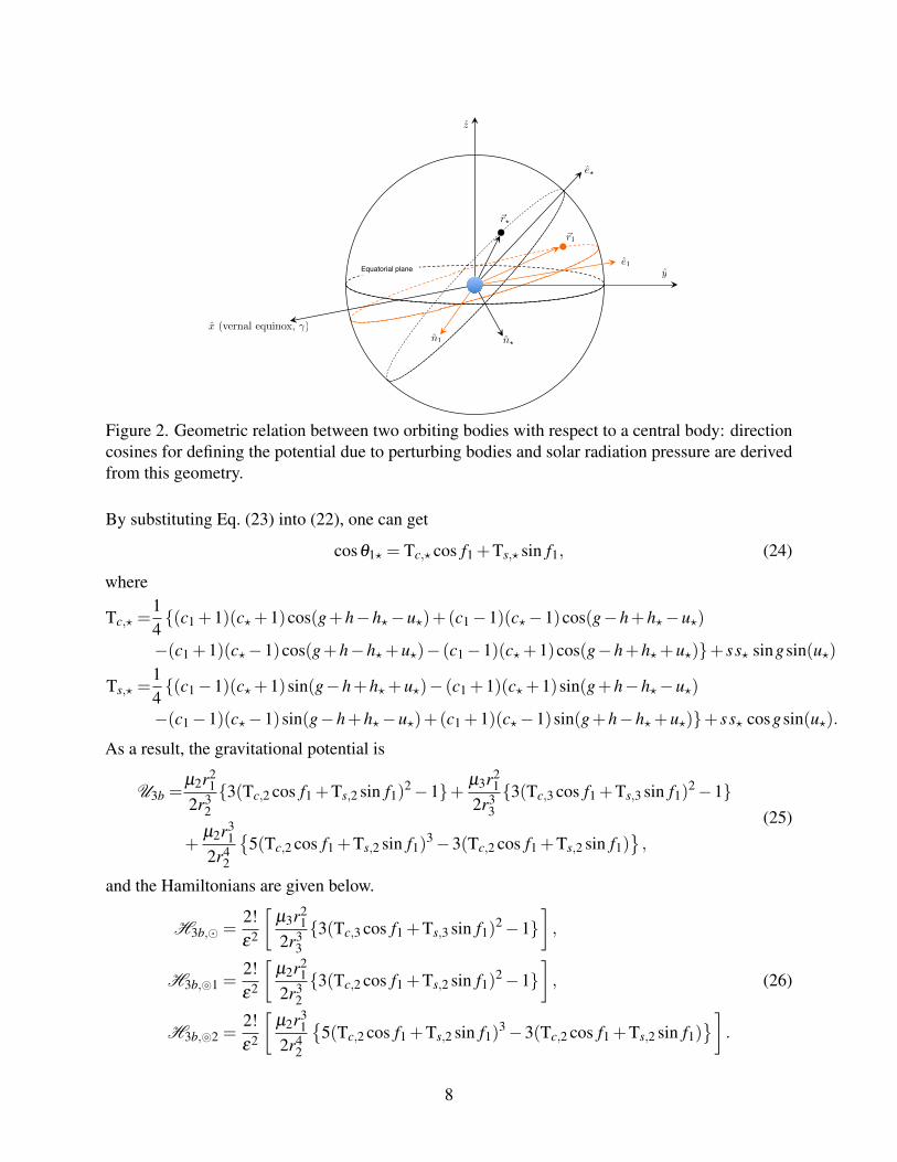
The angular distance θ1m is the included angle between the position vectors of the satellite andm-th perturbing body. The next step is to express Eq. (22) in terms of the orbital elements. Thisstep is carried out based on Fig. 2, and the position vectors is rewritten in Eq. (23) (u? = f?+g?).

rrr1 =

cosh1 cos( f1 +g1)− cos i1 sinh1 sin( f1 +g1)cos i1 cosh1 sin( f1 +g1)+ sinh1 cos( f1 +g1)

sin i1 sin( f1 +g1)

rrr? =

cosh? cosu?− cos i? sinh? sinu?cos i? cosh? sinu?+ sinh? cosu?

sin i? sinu?

(23)

1A more detailed procedure for rewriting Eq. (20) to (21) can be found in [17].

7

Equatorial plane y

z

x (vernal equinox, )

~r?

~r1

e?

n?n1

e1

Figure 2. Geometric relation between two orbiting bodies with respect to a central body: directioncosines for defining the potential due to perturbing bodies and solar radiation pressure are derivedfrom this geometry.

By substituting Eq. (23) into (22), one can get

cosθ1? = Tc,? cos f1 +Ts,? sin f1, (24)

where

Tc,? =14(c1 +1)(c?+1)cos(g+h−h?−u?)+(c1−1)(c?−1)cos(g−h+h?−u?)

−(c1 +1)(c?−1)cos(g+h−h?+u?)− (c1−1)(c?+1)cos(g−h+h?+u?)+ ss? singsin(u?)

Ts,? =14(c1−1)(c?+1)sin(g−h+h?+u?)− (c1 +1)(c?+1)sin(g+h−h?−u?)

−(c1−1)(c?−1)sin(g−h+h?−u?)+(c1 +1)(c?−1)sin(g+h−h?+u?)+ ss? cosgsin(u?).

As a result, the gravitational potential is

U3b =µ2r2

1

2r323(Tc,2 cos f1 +Ts,2 sin f1)

2−1+ µ3r21

2r333(Tc,3 cos f1 +Ts,3 sin f1)

2−1

+µ2r3

12r4

2

5(Tc,2 cos f1 +Ts,2 sin f1)

3−3(Tc,2 cos f1 +Ts,2 sin f1),

(25)

and the Hamiltonians are given below.

H3b, =2!ε2

[µ3r2

1

2r333(Tc,3 cos f1 +Ts,3 sin f1)

2−1],

H3b,1 =2!ε2

[µ2r2

1

2r323(Tc,2 cos f1 +Ts,2 sin f1)

2−1],

H3b,2 =2!ε2

[µ2r3

12r4

2

5(Tc,2 cos f1 +Ts,2 sin f1)

3−3(Tc,2 cos f1 +Ts,2 sin f1)]

.

(26)

8

4.3. Solar Radiation Pressure

The Hamiltonian for the SRP is[21]

Hs =−βr

r2,sat

cosθ13, (27)

whereβ = (1+ρ)

Asat

msatPΦ.

β represents the solar perturbation strength. The solar constant, PΦ, is approximately 1×108 kgkm3/s2/m2

[24]. We assume that the reflectivity (ρ) and area-to-mass ratio (Asat/msat) are 0.2 and 2.0 m2/kg,respectively. From Eq. (24), the Hamiltonian becomes

Hs =4!ε4

[−β

r1

r213

(Tc,3 cos f1 +Ts,3 sin f1)

]. (28)

5. Simulations

The hybrid method is tested with two scenarios: a Medium-Earth-Orbit (MEO) and a highlyelliptical orbit (Molniya). These cases demonstrate the capabilities of the proposed method whenpropagating the state uncertainty, including the multiple perturbations discussed above. The initialconditions are chosen to avoid singularity problems, e.g., zero eccentricity, zero inclination, andcritical inclination, because the current hybrid method is defined in terms of the Delaunay variables.Table 1 presents the initial orbit conditions for each case. The ephemerides of the Sun and moonhave been obtained from the JPL ephemeris file (DE405) from January 19, 2008 00:00:00 UCT toFebruary 2, 2008, 23:59:59 UCT (15 days), which covers the period studied. For the Monte Carlo

Table 1. Initial Keplerian elements for RSOs on MEO and Molniya orbitMEO Molniya

Semimajor axis, a, (km) 26578.14 26578.14Eccentricity, e 0.01 0.74

Inclination, i, (deg) 55 63Longitude of the ascending node, Ω, (deg) 45 45

Argument of periapsis, ω , (deg) 60 270Mean anomaly, l, (deg) 105 105

simulation, normally distributed 30,000 samples within a specified 3-σ region are generated withrespect to the given initial condition. A Gaussian error (1-σ ) is assumed with standard deviationsof 10 km in the semi-major axis, 0.05 in eccentricity, and 0.01 in the inclination, longitude ofascending node, the argument of the pericenter, and the mean anomaly directions. The samples arepropagated for 30-orbital periods (≈ 15 days.) A propagated uncertainty from the Monte-Carlosimulation with the full dynamics is assumed as the truth. The ode45 function in MATLAB is usedas a numerical integrator. In this section, we verify the accuracy of the hybrid method throughtwo statistical methods. Then, we compare an elapse time of the hybrid method to those from theMonte-Carlo simulation with the full dynamics and with the SDS itself to show the improvement ofcomputational efficiency.

9

5.1. Result I: Verification of the Accuracy

5.1.1. Uncertainty for Highly Elliptical Orbit Objects from the Hybrid Method

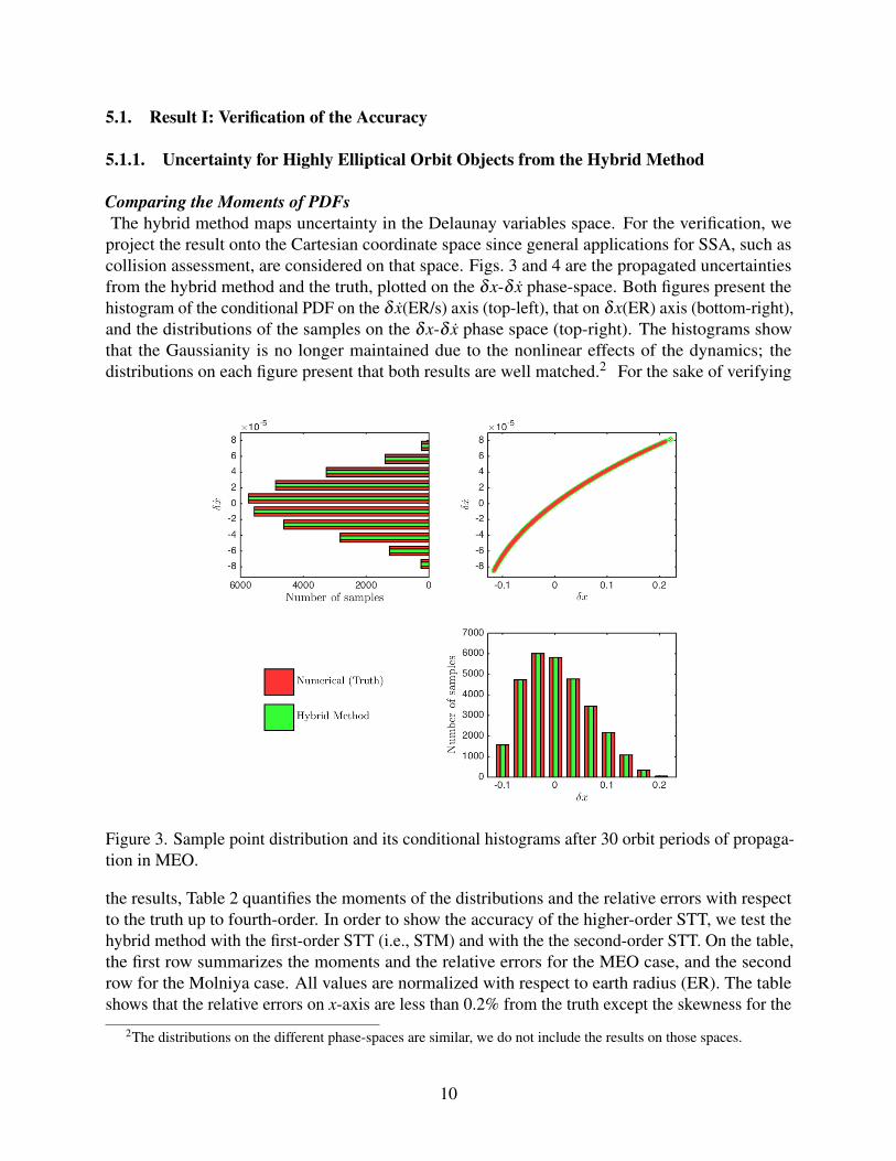
Comparing the Moments of PDFsThe hybrid method maps uncertainty in the Delaunay variables space. For the verification, we

project the result onto the Cartesian coordinate space since general applications for SSA, such ascollision assessment, are considered on that space. Figs. 3 and 4 are the propagated uncertaintiesfrom the hybrid method and the truth, plotted on the δx-δ x phase-space. Both figures present thehistogram of the conditional PDF on the δ x(ER/s) axis (top-left), that on δx(ER) axis (bottom-right),and the distributions of the samples on the δx-δ x phase space (top-right). The histograms showthat the Gaussianity is no longer maintained due to the nonlinear effects of the dynamics; thedistributions on each figure present that both results are well matched.2 For the sake of verifying

Figure 3. Sample point distribution and its conditional histograms after 30 orbit periods of propaga-tion in MEO.

the results, Table 2 quantifies the moments of the distributions and the relative errors with respectto the truth up to fourth-order. In order to show the accuracy of the higher-order STT, we test thehybrid method with the first-order STT (i.e., STM) and with the the second-order STT. On the table,the first row summarizes the moments and the relative errors for the MEO case, and the secondrow for the Molniya case. All values are normalized with respect to earth radius (ER). The tableshows that the relative errors on x-axis are less than 0.2% from the truth except the skewness for the

2The distributions on the different phase-spaces are similar, we do not include the results on those spaces.

10

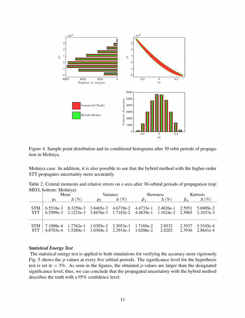
Figure 4. Sample point distribution and its conditional histograms after 30 orbit periods of propaga-tion in Molniya.

Molniya case. In addition, it is also possible to see that the hybrid method with the higher-orderSTT propagates uncertainty more accurately.

Table 2. Central moments and relative errors on x-axis after 30-orbital periods of propagation (top:MEO, bottom: Molniya)

Mean Variance Skewness Kurtosisµ1 ∆ (%) µ2 ∆ (%) µ3 ∆ (%) µ4 ∆ (%)

STM 6.5518e-3 8.3259e-3 3.8465e-3 4.6719e-2 4.4733e-1 2.4626e-1 2.5951 5.6909e-2STT 6.5509e-3 2.1223e-3 3.8476e-3 1.7182e-2 4.4839e-1 1.1624e-2 2.5965 2.1037e-3

STM 7.1008e-4 1.7762e-1 1.0305e-2 2.3053e-1 1.7169e-2 2.8532 2.3937 5.5345e-4STT 6.8703e-4 1.5280e-1 1.0304e-2 2.2914e-1 1.6206e-2 2.8202 2.3936 2.8641e-4

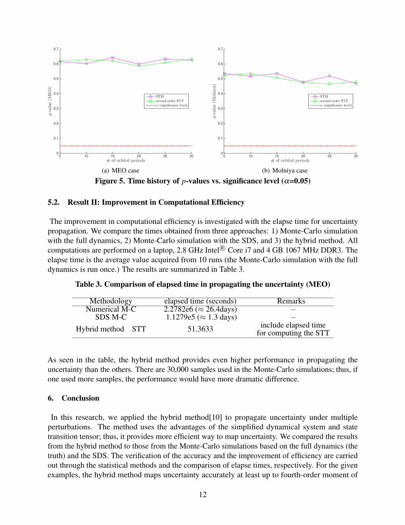
Statistical Energy TestThe statistical energy test is applied to both simulations for verifying the accuracy more rigorously.Fig. 5 shows the p-values at every five orbital periods. The significance level for the hypothesistest is set α = 5%. As seen in the figures, the obtained p-values are larger than the designatedsignificance level; thus, we can conclude that the propagated uncertainty with the hybrid methoddescribes the truth with a 95% confidence level.

11

# of orbital periods5 10 15 20 25 30

p-value(M

EO)

0

0.1

0.2

0.3

0.4

0.5

0.6

0.7

STMsecond-order STTα (significance level)

(a) MEO case

# of orbital periods5 10 15 20 25 30

p-value(M

olniya)

0

0.1

0.2

0.3

0.4

0.5

0.6

0.7

STMsecond-order STTα (significance level)

(b) Molniya case

Figure 5. Time history of p-values vs. significance level (α=0.05)

5.2. Result II: Improvement in Computational Efficiency

The improvement in computational efficiency is investigated with the elapse time for uncertaintypropagation. We compare the times obtained from three approaches: 1) Monte-Carlo simulationwith the full dynamics, 2) Monte-Carlo simulation with the SDS, and 3) the hybrid method. Allcomputations are performed on a laptop, 2.8 GHz Intel R© Core i7 and 4 GB 1067 MHz DDR3. Theelapse time is the average value acquired from 10 runs (the Monte-Carlo simulation with the fulldynamics is run once.) The results are summarized in Table 3.

Table 3. Comparison of elapsed time in propagating the uncertainty (MEO)

Methodology elapsed time (seconds) RemarksNumerical M-C 2.2782e6 (≈ 26.4days) −

SDS M-C 1.1279e5 (≈ 1.3 days) −Hybrid method STT 51.3633 include elapsed time

for computing the STT

As seen in the table, the hybrid method provides even higher performance in propagating theuncertainty than the others. There are 30,000 samples used in the Monte-Carlo simulations; thus, ifone used more samples, the performance would have more dramatic difference.

6. Conclusion

In this research, we applied the hybrid method[10] to propagate uncertainty under multipleperturbations. The method uses the advantages of the simplified dynamical system and statetransition tensor; thus, it provides more efficient way to map uncertainty. We compared the resultsfrom the hybrid method to those from the Monte-Carlo simulations based on the full dynamics (thetruth) and the SDS. The verification of the accuracy and the improvement of efficiency are carriedout through the statistical methods and the comparison of elapse times, respectively. For the givenexamples, the hybrid method maps uncertainty accurately at least up to fourth-order moment of

12

PDFs and 95% of the confidence level with only 0.002% of the elapse time of the Monte-Carlosimulation with the full dynamics. Therefore, we can conclude that the hybrid method propagatesuncertainty accurately and efficiently under the given multiple perturbing environment.

7. References

[1] Junkins, J. L., Akella, M. R., and Alfriend, K. T. “Non-Gaussian Error Propagation inOrbital Mechanics.” Journal of Astronautical Sciences, Vol. 44, No. 4, pp. 541–563, October-December 1996.

[2] Park, R. S. and Scheeres, D. J. “Nonlinear Mapping of Gaussian Statistics: Theory andApplications to Spacecraft Trajectory Design.” Journal of Guidance, Control, and Dynamics,Vol. 29, No. 6, pp. 1367–1375, November-December 2006. doi:10.2514/1.20177.

[3] Tapley, B. D., Schutz, B. E., and Born, G. H. Statistical Orbit Determination. ElsevierAcademic Press, Burlington, MA, 1 edn., 2004.

[4] Maybeck, P. S. Stochastic Models, Estimation and Control, Vol. 2. Academic Press, NewYork, NY, 1982.

[5] Jones, B. A., Doostan, A., and Born, G. H. “Nonlinear Propagation of Orbit Uncertainty UsingNon-Intrusive Polynomial Chaos.” Journal of Guidance, Control, and Dynamics, Vol. 36,No. 2, pp. 430–444, March-April 2013. doi:10.2514/1.57599.

[6] Horwood, J. T., Aragon, N. D., and Poore, A. B. “Gaussian Sum Filters for Space Surveillance:Theory and Simulations.” Journal of Guidance, Control, and Dynamics, Vol. 34, No. 6, pp.1839–1851, December 2011. doi:10.2514/1.53793.

[7] Terejanu, G., Singla, P., Singh, T., and Scott, P. D. “Uncertainty Propagation for NonlinearDynamic Systems Using Gaussian Mixture Models.” Journal of Guidance, Control, andDynamics, Vol. 31, No. 6, pp. 1623–1633, November-December 2008. doi:10.2514/1.36247.

[8] Giza, D., Singla, P., and Jah, M. “An approach for Nonlinear Uncertainty Propagation:Application to Orbital Mechanics.” AIAA 2009-6082. AIAA, 2009.

[9] DeMars, K. J. Nonlinear Orbit Uncertainty Prediction and Rectification for Space SituationalAwareness. thesis, University of Texas at Austin, December 2010.

[10] Park, I. and Scheeres, D. J. “The New Method for Nonlinear Propagation of Uncertainty forNon-Keplerian Motion (in preparation).” Journal of Guidance, Control, and Dynamics, 2015.

[11] Park, I., Scheeres, D. J., and Fujimoto, K. “The Effect of Dynamical Accuracy for Uncer-tainty Propagation.” S. B. Broschart, J. D. Turner, K. C. Howell, and F. R. Hoots, editors,“Astrodynamics 2013,” Vol. 150. August 2013.

13

[12] Fujimoto, K. and Scheeres, D. J. “Analytical Nonlinear Propagation of Uncertainty in the Two-Body Problem.” Journal of Guidance, Control, and Dynamics, Vol. 35, No. 2, pp. 497–509,2012. doi:10.2514/1.54385.

[13] Park, I. and Scheeres, D. J. “The Effect of Dynamical Accuracy for Uncertainty Propagation(accepted).” Journal of Guidance, Control, and Dynamics, 2015.

[14] Deprit, A. “Canonical Transformations Depending on a Small Parameter.” Celestial Mechanics,Vol. 1, pp. 12–30, 1969.

[15] Aslan, B. and Zech, G. “Statistical energy as a tool for binning-free, multivariate goodness-of-fit tests, two-sample comparison and unfolding.” Nuclear Instruments and Methods in PhysicsResearch, Vol. 537, pp. 626–636, 2005. doi:10.1016/j.nima.2004.08.071.

[16] Aslan, B. The concept of energy in nonparametric statistics - Goodness-of-Fit problems anddeconvolution. Ph.D. thesis, Universitat Siegen, 2004.

[17] Roy, A. E. Orbital Motion. Taylor and Francis Group, fourth edn., 2005.

[18] Kamel, A. A. “Perturbation Method in the Theory of Nonlinear Oscillations.” CelestialMechanics, Vol. 3, pp. 90–106, 1970.

[19] Grimmett, G. and Stirzaker, D. Probability and Random Processes. Oxford, England: OxfordUniversity Press, 3rd edn., 2009. ISBN 978-0198572220.

[20] Szekely, G. J. and Rizzo, M. L. “Energy Statistics: A Class of Statistics Based on Distances.”Journal of Statistical Planning and Interference, Vol. 143, pp. 1249–1272, 2013. doi:10.1016/j.jspi.2013.03.018.

[21] Hori, G. I. “The effect of radiation pressure on the motion of an artificial satellite.” J. B.Rosser, editor, “Space Mathematics Part 3,” Vol. 7, pp. 167–182. American MathematicalSociety, 1966.

[22] Saad, N. A., Khalil, K. I., and Amin, M. Y. “Analytical Solution for the Combined SolarRadiation Pressure and Luni-Solar Effects on the Orbits of High Altitude Satellites.” TheOpen Astronomy Journal, Vol. 3, pp. 113–122, 2010.

[23] Brouwer, D. “Solution of the Problem of Artificial Satellite Theory without Drag.” TheAstronomical Journal, Vol. 64, No. 1274, pp. 378–396, 1959.

[24] Scheeres, D. J. Orbital Motion in Strongly Perturbed Environments. Springer, 2012.

14