A Hybrid Finite Difference Method for ValuingAmerican Puts

Jin Zhang∗ SongPing Zhu †

Abstract—This paper presents a numerical schemethat avoids iterations to solve the nonlinear partialdifferential equation system for pricing American putswith constant dividend yields. Upon applying a front-fixing technique to the Black-Scholes partial differen-tial equation, a predictor-corrector finite differencescheme is proposed to numerically solve the discretenonlinear scheme. In the comparison with the solu-tions from articles that cover zero dividend and con-stant dividend yields cases, our results are found accu-rate. The current method is conditionally stable sincethe Euler scheme is used, the convergency propertyof the scheme is shown by numerical experiments.

Keywords:American Options, Predictor-Corrector, Fi-

nite Difference Method, Black-Scholes Equation

1 Introduction

Options are the most common securities that are fre-quently bought and sold in today’s financial markets. Un-der the Black-Scholes partial differential equation (PDE)framework, Merton [1] casts the valuation problem ofAmerican options as a free-boundary problem in 1973.Ever since then, there have been two kinds of approx-imation methods in the literature, to solve the free-boundary problem associated with the valuation of Amer-ican options. One approach is the analytical approxima-tion method, e.g. the Quasi-analytical formula [2]. Theother one is the numerical method, such as the BinomialMethod [3], which are quite preferred by market practi-tioners, as they are usually much faster with acceptableaccuracy.

In the last decade, various numerical methods have beenpresented by using the finite difference method (FDM),to solve the pricing problems of American options. Forinstance, Wu and Kwok [5] use a multilevel FDM to solvethe nonlinear Black-Scholes PDE after applying a front-fixing technique [6], they adopt a so-called front-fixingtechnique or Landau transform [6] to fix the optimal ex-ercise boundary on a vertical axis. To tackle the nonlin-

∗Centre for Computational Finance and Economic Agents, Uni-versity of Essex, United Kingdom. Email:jzhangf@essex.ac.uk. Theauthor gratefully acknowledges the financial support from the EUCommission through MRTNCT2006034270 COMISEF for attend-ing this conference.

†School of Mathematics and Applied Statistics, University ofWollongong, Australia. Email: songping zhu@uow.edu.au

ear nature of American option pricing problems, whichis explicitly exposed after applying the front-fixing tech-nique [6] to the original Black-Scholes PDE, they employa two-level discretization scheme in time. However, sincethe scheme is a multilevel discretization scheme, the in-formation at more than one time step is needed at thebeginning to start the computation, which is referred toas the initialization for multilevel schemes in literature.The multilevel scheme of Wu and Kwok [5] motivates usa simpler version, while maintains the same level of com-putational accuracy.

To avoid the initialization and iteration, we propose aone-step scheme based on a prediction-correction frame-work. The approach adopts a predictor-corrector finitedifference scheme at each time step to convert the non-linear PDE to two linearized difference equations asso-ciated with the prediction and correction phase respec-tively. The predictor is constructed by an explicit Eulerscheme, whereas the corrector is designed with the Crank-Nicolson scheme. The predictor is used only to calculatethe optimal exercise price, as the literature shows that itis far more difficult to calculate the optimal exercise pricewith a high accuracy. The predicted optimal exerciseprice is then corrected in the correction phase togetherwith the calculation of the option prices. The schememaximizes the use of computational resources, as a highaccuracy of the computed option price is easy to achieveas long as a high accuracy can be achieved in the compu-tation of the optimal exercise price. The efficiency in thescheme results from the fact that only one set of linearalgebraic equations needs to be solved at each time step.

The paper is organized as follows. Section 2 introducesthe PDE system concerning the valuation of Americanput options. Section 3 presents a predictor-correctorscheme for computing the optimal exercise prices and theoption values. In Section 4, some numerical examples aregiven to demonstrate the convergence and accuracy of thenew scheme. Section 5 draws conclusions.

2 Partial Differential Equation System

This paper considers a general case in which a constantdividend yield is associated with the underlying asset andadopt the PDE given in Merton [1]. Let V denote thevalue of an American put option, which is a function of

Proceedings of the World Congress on Engineering 2009 Vol IIWCE 2009, July 1 - 3, 2009, London, U.K.

ISBN:978-988-18210-1-0 WCE 2009

the value of underlying asset S and the time t. The valueof an American put option also depends on the followingparameters:σ, the volatility of the underlying asset;T , the life time of the contract;X, the strike price;r, the risk-free interest rate;D0, the dividend yield.Without loss of generality, we assume that both the risk-free interest rate and the dividend yield be constants.The functions can be easily modified for the cases whenthey are some known functions of time and asset values.

Since American options can be decomposed into its Eu-ropean counterparts plus an early exercise premium, thisearly exercise premium is associated with the extra rightembedded in American options in comparison with itsEuropean counterparts. Wilmott et al. [9] show thatthere are two boundary conditions of the optimal exer-cise price S = Sf (t) for American options:

{V (Sf (t), t) = X − Sf (t),∂V∂S (Sf (t), t) = −1.

(1)

To close the system, another boundary condition at theend of large asset value, i.e. the payoff of the contract atthe expiry is necessary,

limS→∞

V (S, t) = 0, (2)

and the terminal condition for a put option is

V (S, T ) = max{X − S, 0}. (3)

In summary, the differential system for pricing Americanput options can be written as:

∂V∂t + 1

2σ2S2 ∂2V∂S2 + (r −D0)S ∂V

∂S − rV = 0,V (Sf (t), t) = X − Sf (t),∂V∂S (Sf (t), t) = −1,limS→∞ V (S, t) = 0,V (S, T ) = max{X − S, 0}.

(4)

To solve the differential system Eq. (4) effectively, wenormalize all variables in the system by introducing thefollowing scale of variables,V ′ = V

X , S′ = SX , τ = (T − t)σ2

2 , γ = 2rσ2 ,

D = 2D0σ2 , S′f (τ) = Sf (T−2τ/σ2)

X .After normalizing Eq. (4), dropping the primes, and im-posing the Landau transform [6],

x = lnS

Sf (τ), (5)

the original system becomes:

∂P∂τ − ∂2P

∂x2 + (γ −D − 1)∂P∂x + γP =

∂P∂x

1Sf (τ)

dSf (τ)dτ ,

P (0, τ) = 1− Sf (τ),∂P∂x (0, τ) = −Sf (τ),limx→∞ P (x, τ) = 0,P (x, 0) = 0.

(6)

After this rather simple manipulation, the nonlinear na-ture of the problem is explicitly exposed in the inhomo-geneous term on the right hand side of Eq. (6), whichconsists the product of the Delta of the unknown optionprice under the Landau transform, the time derivativeof the unknown optimal exercise boundary Sf (τ) and itsreciprocal.

One should note that we have replaced the unknown func-tion V (S, t) in Eq. (4), with a new unknown function P ,which is defined as P (x, τ) = V (S(x, (τ)), τ) through thetransform defined in Eq. (5). This is to facilitate the in-troduction of a relation between P (0, τ) and the Sf (τ) onthe boundary x = 0, which is used to design the predictorof the numerical scheme. Moreover, one should also notethat the transform in Eq. (5) only holds if Sf (τ) > 0.This condition poses no problem since it is easy to showthat the Sf (τ) for an American put option is a monoton-ically decreasing function of τ ; the minimum value Sf (τ)is the optimal exercise price of the corresponding perpet-ual contract. For a perpetual American put on a constantdividend yield paying asset, this value was shown as fol-lows:

limτ→∞

Sf (τ) =η +

√η2 + 4γ

2 + η +√

η2 + 4γ, (7)

with η = γ −D − 1. It is then very trivial to show thatSf (τ) > 0 for any η values. Therefore, the differentialsystem Eq. (5) defines a well-posed problem, other thana well-known singular point at τ = 0 (see Barles et al.[10]). We now propose an efficient and accurate numericalscheme to solve this system.

3 The Predictor-Corrector FDM Scheme

This section presents the predictor-corrector scheme. Wepropose to solve the nonlinear PDE in differential systemEq. (6) in two phases within a time step, a predictionphase in which an initial guess of the Sf (τ) is worked outbefore its final value is calculated together with the optionvalue P (x, τ) in the correction phase of the scheme.

Beginning with truncating the bounded x domain, as wellas the time domain τ , the computational domain is dis-cretized with uniformly spread M + 1 grids placed in thex direction and N + 1 grids in the τ direction (i.e., Mand N are the number of steps in these two directions,respectively). For the easiness of presentation, we denotethe step length in the x direction by ∆x = xmax

M andthat in the τ direction by ∆τ = τexp

N , in which τexp is thenormalized tenor of the contract with respect to half ofthe variance of the underlying asset, i.e., τexp = Tσ2/2.Consequently, the value of unknown function P at a gridpoint is denoted by Pn

m with the superscript n denotingthe nth time step and the subscript m denoting the mthlog-transformed asset grid point.

To facilitate the numerical computation, we derive an ad-

Proceedings of the World Congress on Engineering 2009 Vol IIWCE 2009, July 1 - 3, 2009, London, U.K.

ISBN:978-988-18210-1-0 WCE 2009

ditional boundary condition to construct our predictor-corrector scheme. This condition is not independent fromall those boundary conditions prescribed in Eq. (6).Rather, it is derived by making use of the PDE in Eq.(6) as well as the boundary conditions that have alreadymade the system closed. Firstly, we take a partial deriva-tive with respect to τ on both sides of the first boundarycondition in Eq. (6), which yields

∂P

∂τ(0, τ) = −dSf (τ)

dτ. (8)

In fact, one easily shows that Eq. (8) is consistent withthe condition ∂V

∂τ (Sf (τ), τ) = 0 in Bunch and Johnson’spaper [7]. Then, if we evaluate the PDE in Eq. (6)at x = 0, utilizing Eq. (8) and the second boundarycondition in Eq. (6), we obtain

∂2P

∂x2 |x=0− (D + 1)Sf (τ) + γ = 0, if τ > 0. (9)

Eq. (9) reveals a relationship of the put option price andthe optimal exercise price at any time, except on the ex-piry day. This relation is important to our scheme ineliminating the value of the unknown function defined onthe fictitious grid point near the boundary x = 0, whenthe second-order central difference scheme is applied. Thereason that it is only valid for τ > 0 is the inherent sin-gular behavior of the Black-Scholes PDE at τ = 0 (seeBarles et al. [10]).

Applying a second-order central difference scheme to theequation, one has the asset price discretization in the xdirection. Eq. (9) and the boundary conditions in Eq.(6) is written as

−Pn+11 − 2Pn+1

0 + Pn+1−1

∆x2− (D +1)Sf

n+1 + γ = 0, (10)

and

Pn+10 = 1− Sf

n+1,P n+1

1 −P n+1−1

2∆x = −Sfn+1,

Pn+1M = 0,

P 0m = 0,

(11)

respectively. Upon eliminating the fictitious nodal valuePn+1−1 from Eq. (10) and the second equation in Eq. (11),

we obtain a relation between Sf and P1 at the (n + 1)thtime step as

Pn+11 = α− βSf

n+1, (12)

in which α = 1 + γ2 ∆x2 and β = 1 + ∆x + D+1

2 ∆x2. Eq.(12) is used in the predictor and corrector construction.

Predictor: The predictor is constructed by using the ex-plicit Euler scheme to calculate a guessed value of Sf

n+1,

which is denoted as Sfn+1

. Applying the explicit Euler

scheme to the PDE in Eq. (6) results in

Pn+11 − Pn

1

∆τ− Pn

2 − 2Pn1 + Pn

0

∆x2 −(γ−D−1)Pn

2 − Pn0

2∆x+

γPn1 =

Pn2 − Pn

0

2∆x

1Sf

n

Sfn+1 − Sf

n

∆τ, (13)

which is coupled with Eq. (12) to generate the Sfn+1

value. The boundary condition of Pn+10 used in the

corrector is also predicted here; with the calculatedSf

n+1value, Pn+1

0 is calculated from the first equationin Eq. (11), which is nothing but the payoff function.Like the predicted Sf

n+1value, this predicted boundary

value of Pn+10 will also be corrected once the Sf

n+1is

corrected in the following corrector scheme.

Corrector: The corrector is based on the Crank-Nicolson scheme, applied to the linearized PDE in Eq.(6). The linearlization is designed with an alternatingterm being valued at the current time step in comparisonwith that in the predictor. In the predictor, we let thetime derivative of the Sf in the nonlinear inhomogeneousterm be valued at the current time step, whereas now welet the asset price derivative of P be valued at the currenttime step through the Crank-Nicolson scheme. Thisalternating approach, inspired by the idea of the ADIapproach in solving two dimensional time-dependentPDEs [11], has an advantage of reducing the numericalerrors induced in the prediction-correction process. Thefinite difference scheme used for the corrector is

Pn+1m − Pn

m

∆τ+ γ

Pn+1m + Pn

m

2−

Pn+1m+1 − 2Pn+1

m + Pn+1m−1 + Pn

m+1 − 2Pnm + Pn

m−1

2∆x2

− (γ −D − 1)Pn+1

m+1 − Pn+1m−1 + Pn

m+1 − Pnm−1

4∆x+

=Pn+1

m+1 − Pn+1m−1 + Pn

m+1 − Pnm−1

4∆x× 2

Sfn+1

+ Sfn

× Sfn+1 − Sf

n

∆τ.

(14)

In Eq. (14), m value starts from 1 to M − 1, which indi-cates that M − 1 equations are solved simultaneously toobtain the corrected option values at the (n + 1)th timestep. Pn+1

1 is obtained upon solving Eq. (14). Then,by means of Eq. (12), the newly-obtained Pn+1

1 is usedto correct the Sf

n+1, which is then used to correct thePn+1

0 value before it is used in the calculation of the nexttime step. And Eq. (14) can be written in matrix formwhich is a more condensed way for Matlab computation.This predictor-corrector process is repeated until the ex-piry time is reached. We solve these matrix equations inMatlab, Version 7 on a Intel P4 machine.

Proceedings of the World Congress on Engineering 2009 Vol IIWCE 2009, July 1 - 3, 2009, London, U.K.

ISBN:978-988-18210-1-0 WCE 2009

4 Numerical Examples

Although the Crank-Nicolson scheme for the corrector isunconditionally stable [11], our predictor-corrector finitedifference scheme is only conditionally stable since theexplicit Euler scheme for the predictor is conditionallystable. In this section, the conditional stability of ourapproach, as well as the accuracy shall be verified empir-ically.

4.1 Discussion on Convergence

For the linearized system, the proof of the consistency istrivial through the application of Taylor’s expansion andthus is omitted here. A theoretical proof the stabilityfor the linearized system, on the other hand, is not sotrivial because of the presence of the singularity at τ = 0(see Barles et al. [10]). Therefore, we establish a stabilitycriterion empirically. Based on preliminary numerical ex-periments, we were convinced that the stability criterion∆τ∆x2 ≤ 1 should be imposed in the selection of time steplength for a given grid size in the x direction. Betweenthe option price and the optimal exercise price, the lat-ter is far more difficult to calculate accurately; once theSf (τ) is determined accurately, the calculation of the op-tion price itself is straight forward. Therefore, in thissubsection we focus on the calculation of the Sf (τ) first.

The example we chose for our numerical tests has beenused by researchers for the discussion of American putson an asset without any dividend payment [4, 5]. The rel-evant parameters are: the strike price X = $100, the in-terest rate r = 10%, the volatility of the underlying assetσ = 30% and the tenor of the option being one year. Inthis subsection, we focus only on the zero-dividend case,i.e., we set the constant dividend yield to zero. For theconvenience of those readers who prefer to see the resultsin dimensional form, all results presented in this sectionare those associated with the original dimensional quan-tities before the normalization process was introduced.

Firstly, we examined a point-wise convergence by focus-ing on a specific point of the Sf value first. As an in-dicator, the differences of Sf values at a specific time toexpiry, say 1 year, are calculated with time step size beingconsecutively halved. Table 1 shows the differences of thecomputed Sf values with the total number of grid pointsin the x direction being fixed to 51, while the numberof time step intervals is consecutively doubled from 200to 3200 (the time step size is consecutively halved). Oneshould note that in Table 1, the “difference” refers to theabsolute change in Sf values when the time step size ishalved, while the “ratio” refers to the ratio of successivedifferences. Theoretically, the order of convergence is re-lated to calculated ratio by ratio = 2k, in which k is theorder of convergence. Clearly, when the grid size in the xdirection is fixed, the ratios of the differences of two Sf

values at τ = 1 year with two consecutive calculations of

Table 1: Ratios for the order of convergence in timeTime steps Sf ($) difference ratio

200 76.126400 76.121 0.00000406800 76.120 0.00000125 3.2611600 76.120 0.00000060 2.0723200 76.119 0.00000030 2.036

Table 2: Ratios for the order of convergence in asset priceGrid intervals Sf ($) difference ratio

50 76.120100 76.150 0.00030017200 76.160 0.00010254 2.927400 76.164 0.00003342 3.068800 76.164 0.00001114 3.000

time step length being halved indeed approach 2, whichindicates that our scheme is indeed of the first order intime.

Then we fixed the time step size to ∆τ = τmax

1600 insteadand examine the ratios of the of the differences of two Sf

values at τ = 1 year with the two consecutive calculationsof x grid length being halved, we find that these ratios areclose to 3, as shown in Table 2. This indicates that theorder of convergence in the x direction is certainly higherthan one but lower than theoretically predicted 2nd orderconvergence of the Crank-Nicolson scheme. One plausi-ble reason for this is that the errors introduced in thepredictor somehow reduced the order of convergence inthe x direction a bit, so that now it is of an order of oneand half rather than two.

Having discussed the point-wise convergence, we testedthe convergence of the new scheme on the entire solutionof Sf . We first ran our code with an extremely fine grid,e.g., the N and M are set up as 102,400 and 1,000, re-spectively. Naturally, this takes a long time to compute.But, once the Sf values are computed on this fine grid,we used these values as the reference values to verify theconvergence of computed Sf values based of some coarsegrid. To measure the overall difference between the re-sults of the coarse grid and those of the finest grid, weuse two error measures. The root mean square absoluteerrors (RMSAE), which is usually referred as root meansquare errors. In order to tell relative errors, a modifica-tion of root mean square errors is used here, we refer itas the root mean square relative errors (RMSRE). Thetwo measures are defined respectively as

RMSAE =

√√√√1I

I∑

i=1

(ai − ai)2, (15)

Proceedings of the World Congress on Engineering 2009 Vol IIWCE 2009, July 1 - 3, 2009, London, U.K.

ISBN:978-988-18210-1-0 WCE 2009

102030405060708090100

50

100

150

200

0

0.01

0.02

0.03

0.04

0.05

0.06

0.07

0.08

Grid Numbers

Time Steps

RM

SA

E

Figure 1: The RMSAE with Increased Grid numbers

102030405060708090100

50

100

150

200

0

0.01

0.02

0.03

0.04

0.05

0.06

0.07

0.08

0.09

0.1

Grid Numbers

Time Steps

RM

SR

E

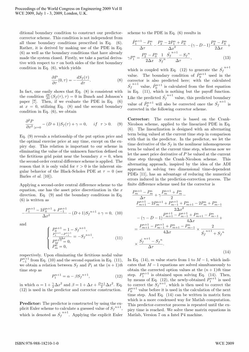
Figure 2: The RMSRE with Increased Grid Numbers

RMSRE =

√√√√1I

I∑

i=1

(ai − ai

ai)2, (16)

where ais are the nodal Sf values associated with coarsegrid; ais are the Sf values associated with finest grid andI is the number of sample points used in the RMSAE andRMSRE. In the following experiments, I was set to be 50for all the results shown in the following diagrams.

By demonstrating the RMSAE and RMSRE, we obtainan overall measure of the convergence to make sure whatwe observed from analyzing the order of convergence pre-viously based on one point only is also true for other gridpoints. Figure 1 and 2 show the RMSAE and RMSRE re-spectively, for the Sf values when the number steps in thex direction and the τ direction are gradually increased.As can be clearly seen from these figures, the RMSAEreduces by nearly 10 folds when the grid size changesfrom N = 10 and M = 10 (with RMSAE = 0.0254)to N = 200 and M = 100 (with RMSAE = 0.0028).In fact, the difference between the results obtained witha coarse grid and those obtained with the finest grid isbetter reflected by the RMSRE, which shows very similartrend as that of the RMSAE; when the number of gridhas increased to N = 200 and M = 100, the RMSRE hasreached 0.3%, which is quite an acceptable accuracy incomparison with the solution based on an extremely re-fined grid. This confirms that analysis of convergence or-der presented earlier can be extended to other grid pointsas well. Therefore, we are confident that the scheme can

0 0.1 0.2 0.3 0.4 0.5 0.6 0.7 0.8 0.9 175

80

85

90

95

100

Time to Expiry (Year)

Opt

imal

Exe

rcis

e P

rice

($)

Solution of current method O Solution of Zhu’s Method

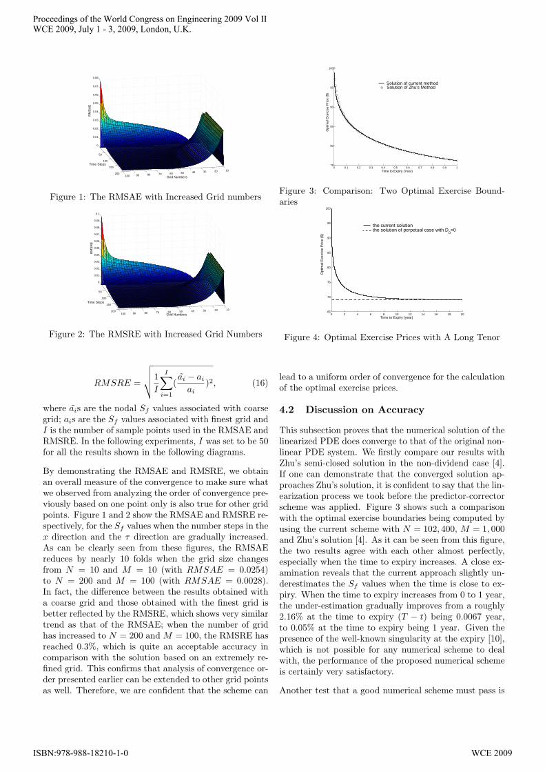
Figure 3: Comparison: Two Optimal Exercise Bound-aries

0 2 4 6 8 10 12 14 16 18 2065

70

75

80

85

90

95

100

Time to Expiry (year)O

ptim

al E

xerc

ise

Pric

e ($

)

the current solution the solution of perpetual case with D

0=0

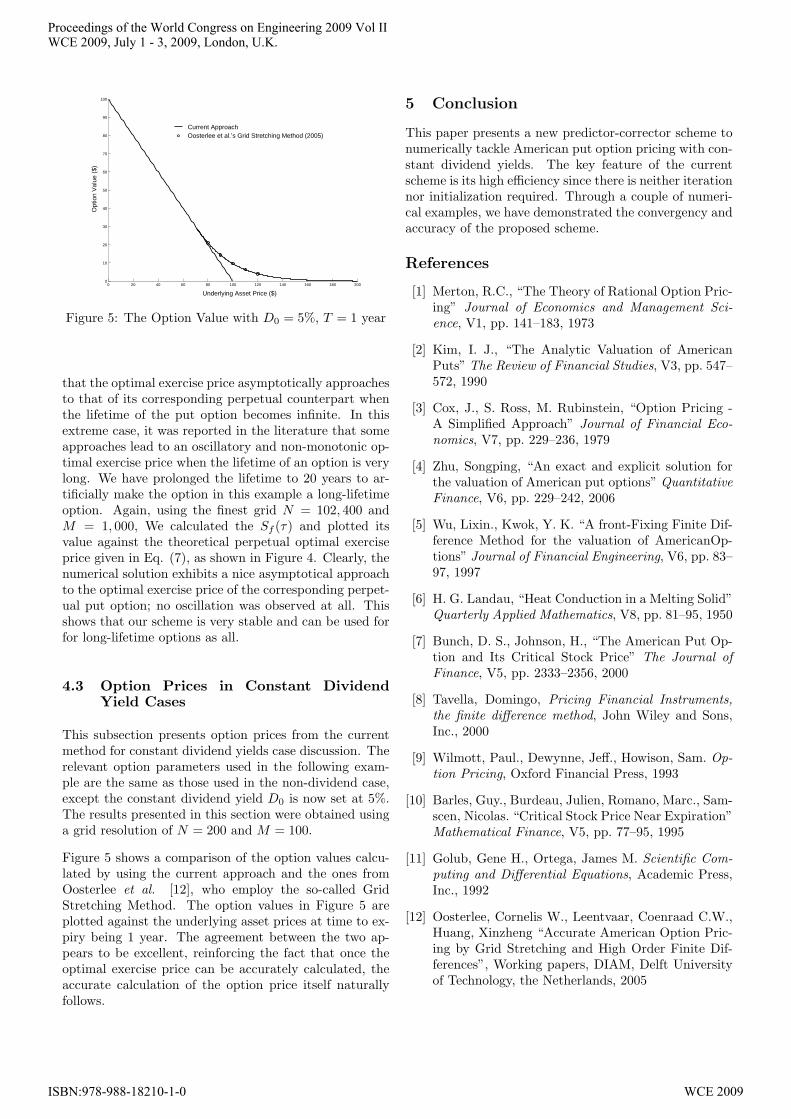
Figure 4: Optimal Exercise Prices with A Long Tenor

lead to a uniform order of convergence for the calculationof the optimal exercise prices.

4.2 Discussion on Accuracy

This subsection proves that the numerical solution of thelinearized PDE does converge to that of the original non-linear PDE system. We firstly compare our results withZhu’s semi-closed solution in the non-dividend case [4].If one can demonstrate that the converged solution ap-proaches Zhu’s solution, it is confident to say that the lin-earization process we took before the predictor-correctorscheme was applied. Figure 3 shows such a comparisonwith the optimal exercise boundaries being computed byusing the current scheme with N = 102, 400, M = 1, 000and Zhu’s solution [4]. As it can be seen from this figure,the two results agree with each other almost perfectly,especially when the time to expiry increases. A close ex-amination reveals that the current approach slightly un-derestimates the Sf values when the time is close to ex-piry. When the time to expiry increases from 0 to 1 year,the under-estimation gradually improves from a roughly2.16% at the time to expiry (T − t) being 0.0067 year,to 0.05% at the time to expiry being 1 year. Given thepresence of the well-known singularity at the expiry [10],which is not possible for any numerical scheme to dealwith, the performance of the proposed numerical schemeis certainly very satisfactory.

Another test that a good numerical scheme must pass is

Proceedings of the World Congress on Engineering 2009 Vol IIWCE 2009, July 1 - 3, 2009, London, U.K.

ISBN:978-988-18210-1-0 WCE 2009

0 20 40 60 80 100 120 140 160 180 2000

10

20

30

40

50

60

70

80

90

100

Underlying Asset Price ($)

Opt

ion

Val

ue (

$)

Current Approach o Oosterlee et al.’s Grid Stretching Method (2005)

Figure 5: The Option Value with D0 = 5%, T = 1 year

that the optimal exercise price asymptotically approachesto that of its corresponding perpetual counterpart whenthe lifetime of the put option becomes infinite. In thisextreme case, it was reported in the literature that someapproaches lead to an oscillatory and non-monotonic op-timal exercise price when the lifetime of an option is verylong. We have prolonged the lifetime to 20 years to ar-tificially make the option in this example a long-lifetimeoption. Again, using the finest grid N = 102, 400 andM = 1, 000, We calculated the Sf (τ) and plotted itsvalue against the theoretical perpetual optimal exerciseprice given in Eq. (7), as shown in Figure 4. Clearly, thenumerical solution exhibits a nice asymptotical approachto the optimal exercise price of the corresponding perpet-ual put option; no oscillation was observed at all. Thisshows that our scheme is very stable and can be used forfor long-lifetime options as all.

4.3 Option Prices in Constant DividendYield Cases

This subsection presents option prices from the currentmethod for constant dividend yields case discussion. Therelevant option parameters used in the following exam-ple are the same as those used in the non-dividend case,except the constant dividend yield D0 is now set at 5%.The results presented in this section were obtained usinga grid resolution of N = 200 and M = 100.

Figure 5 shows a comparison of the option values calcu-lated by using the current approach and the ones fromOosterlee et al. [12], who employ the so-called GridStretching Method. The option values in Figure 5 areplotted against the underlying asset prices at time to ex-piry being 1 year. The agreement between the two ap-pears to be excellent, reinforcing the fact that once theoptimal exercise price can be accurately calculated, theaccurate calculation of the option price itself naturallyfollows.

5 Conclusion

This paper presents a new predictor-corrector scheme tonumerically tackle American put option pricing with con-stant dividend yields. The key feature of the currentscheme is its high efficiency since there is neither iterationnor initialization required. Through a couple of numeri-cal examples, we have demonstrated the convergency andaccuracy of the proposed scheme.

References

[1] Merton, R.C., “The Theory of Rational Option Pric-ing” Journal of Economics and Management Sci-ence, V1, pp. 141–183, 1973

[2] Kim, I. J., “The Analytic Valuation of AmericanPuts” The Review of Financial Studies, V3, pp. 547–572, 1990

[3] Cox, J., S. Ross, M. Rubinstein, “Option Pricing -A Simplified Approach” Journal of Financial Eco-nomics, V7, pp. 229–236, 1979

[4] Zhu, Songping, “An exact and explicit solution forthe valuation of American put options” QuantitativeFinance, V6, pp. 229–242, 2006

[5] Wu, Lixin., Kwok, Y. K. “A front-Fixing Finite Dif-ference Method for the valuation of AmericanOp-tions” Journal of Financial Engineering, V6, pp. 83–97, 1997

[6] H. G. Landau, “Heat Conduction in a Melting Solid”Quarterly Applied Mathematics, V8, pp. 81–95, 1950

[7] Bunch, D. S., Johnson, H., “The American Put Op-tion and Its Critical Stock Price” The Journal ofFinance, V5, pp. 2333–2356, 2000

[8] Tavella, Domingo, Pricing Financial Instruments,the finite difference method, John Wiley and Sons,Inc., 2000

[9] Wilmott, Paul., Dewynne, Jeff., Howison, Sam. Op-tion Pricing, Oxford Financial Press, 1993

[10] Barles, Guy., Burdeau, Julien, Romano, Marc., Sam-scen, Nicolas. “Critical Stock Price Near Expiration”Mathematical Finance, V5, pp. 77–95, 1995

[11] Golub, Gene H., Ortega, James M. Scientific Com-puting and Differential Equations, Academic Press,Inc., 1992

[12] Oosterlee, Cornelis W., Leentvaar, Coenraad C.W.,Huang, Xinzheng “Accurate American Option Pric-ing by Grid Stretching and High Order Finite Dif-ferences”, Working papers, DIAM, Delft Universityof Technology, the Netherlands, 2005

Proceedings of the World Congress on Engineering 2009 Vol IIWCE 2009, July 1 - 3, 2009, London, U.K.

ISBN:978-988-18210-1-0 WCE 2009