
A highly metamorphic virus generator - The Team for Research in
26
402 Int. J. Multimedia Intelligence and Security, Vol. 1, No. 4, 2010 Copyright © 2010 Inderscience Enterprises Ltd. A highly metamorphic virus generator Priti Desai Symantec Corporation, 350 Ellis Street, Mountain View, California, USA E-mail: [email protected] Mark Stamp* Department of Computer Science, San Jose State University, One Washington Square, San Jose, California, USA E-mail: [email protected] *Corresponding author Abstract: Metamorphic viruses modify their code to produce viral copies that are syntactically different from their parents. The viral copies have the same functionality as the parent but typically have no common signature. This makes signature-based virus scanners ineffective for detecting metamorphic viruses. But machine learning tool such as Hidden Markov Models (HMMs) have proven effective at detecting metamorphic viruses. Previous research has shown that most metamorphic generators do not produce a significant degree of metamorphism. In this project, we develop a metamorphic engine that yields highly diverse morphed copies of a base virus. We show that our metamorphic engine easily defeats commercial virus scanners. We then show that, perhaps surprisingly, HMM-based detection is effective against our highly metamorphic viruses. We conclude with a discussion of possible improvements to our generator that might enable it to defeat statistical-based detection methods, such as those that rely on HMMs. Keywords: metamorphic virus; Hidden Markov Model; HMM; anti-virus. Reference to this paper should be made as follows: Desai, P. and Stamp, M. (2010) ‘A highly metamorphic virus generator’, Int. J. Multimedia Intelligence and Security, Vol. 1, No. 4, pp.402–427. Biographical notes: Priti Desai is currently a Software Engineer at Symantec and her main interests are in the area of information security. Prior to this, she obtained her MS in Computer Science from San Jose State University where she developed the metamorphic generator discussed in this paper. Mark Stamp has 20 years of experience in information security. He can neither confirm nor deny that he spent seven years as a cryptanalyst with the National Security Agency, but he can confirm that he worked for two years designing and developing a digital rights management product at a small Silicon Valley start-up company. He is currently an Associate Professor in the Department of Computer Science at San Jose State University where he teaches courses on information security. He has written numerous research papers and two textbooks, Information Security: Principles and Practice, 2nd ed., published by Wiley Interscience in 2011 and Applied Cryptanalysis: Breaking Ciphers in the Real World published by Wiley-IEEE Press in 2007.
Transcript of A highly metamorphic virus generator - The Team for Research in

402 Int. J. Multimedia Intelligence and Security, Vol. 1, No. 4, 2010
Copyright © 2010 Inderscience Enterprises Ltd.
A highly metamorphic virus generator
Priti Desai Symantec Corporation, 350 Ellis Street, Mountain View, California, USA E-mail: [email protected]
Mark Stamp* Department of Computer Science, San Jose State University, One Washington Square, San Jose, California, USA E-mail: [email protected] *Corresponding author Abstract: Metamorphic viruses modify their code to produce viral copies that are syntactically different from their parents. The viral copies have the same functionality as the parent but typically have no common signature. This makes signature-based virus scanners ineffective for detecting metamorphic viruses. But machine learning tool such as Hidden Markov Models (HMMs) have proven effective at detecting metamorphic viruses. Previous research has shown that most metamorphic generators do not produce a significant degree of metamorphism. In this project, we develop a metamorphic engine that yields highly diverse morphed copies of a base virus. We show that our metamorphic engine easily defeats commercial virus scanners. We then show that, perhaps surprisingly, HMM-based detection is effective against our highly metamorphic viruses. We conclude with a discussion of possible improvements to our generator that might enable it to defeat statistical-based detection methods, such as those that rely on HMMs.
Keywords: metamorphic virus; Hidden Markov Model; HMM; anti-virus.
Reference to this paper should be made as follows: Desai, P. and Stamp, M. (2010) ‘A highly metamorphic virus generator’, Int. J. Multimedia Intelligence and Security, Vol. 1, No. 4, pp.402–427.
Biographical notes: Priti Desai is currently a Software Engineer at Symantec and her main interests are in the area of information security. Prior to this, she obtained her MS in Computer Science from San Jose State University where she developed the metamorphic generator discussed in this paper.
Mark Stamp has 20 years of experience in information security. He can neither confirm nor deny that he spent seven years as a cryptanalyst with the National Security Agency, but he can confirm that he worked for two years designing and developing a digital rights management product at a small Silicon Valley start-up company. He is currently an Associate Professor in the Department of Computer Science at San Jose State University where he teaches courses on information security. He has written numerous research papers and two textbooks, Information Security: Principles and Practice, 2nd ed., published by Wiley Interscience in 2011 and Applied Cryptanalysis: Breaking Ciphers in the Real World published by Wiley-IEEE Press in 2007.

A highly metamorphic virus generator 403
1 Introduction
There are many antivirus defence mechanisms available today, but chief among these is signature detection. Metamorphic viruses, that is, viruses that change their ‘appearance’ while maintaining their functionality, represent a powerful technique for evading signature detection. A metamorphic ‘engine’ uses a variety of code morphing techniques to change the structure of the viral code without altering its function.
In Stamp and Wong (2006) and Attaluri et al. (2008), Hidden Markov Models (HMMs) are used to detect metamorphic viruses – including metamorphic viruses that evaded detection by commercial signature-based scanners. An HMM is a machine learning technique and HMMs have a lengthy history of success in applications such as speech recognition and protein modelling.
In this paper, our primary goal is to develop a metamorphic generator that produces the most highly metamorphic viruses yet seen. We then investigate whether the resulting metamorphic viruses can evade both signature detection and HMM-based detection. Our results for the HMM-based detection scheme are, perhaps, somewhat surprising.
This paper is organised as follows: Section 2 provides background information on computer viruses. Section 3 discusses common anti-virus technologies, while Section 4 contains information about the evolution of computer viruses. In Section 5, various code morphing techniques are briefly discussed. Section 6 covers a ‘similarity test’ that we use to measure the effectiveness of our code morphing, and Section 7 gives an abbreviated introduction to HMMs. Sections 8 and 9 detail the design, implementation, and experimental results for our metamorphic engine. Section 10 draws conclusions and discusses future work.
2 Computer virus
Aycock (2006) states a computer virus consists of three parts, as illustrated in Figure 1.
Figure 1 Pseudo code of a computer virus
def virus(): infect () if trigger () is true then payload ()
Figure 2 Pseudo code of infect module
def infect(): repeat k times: target = select_target() if no target then return infect_code (target)
The infect module, which is further illustrated in Figure 2, defines how a virus spreads, where the most common infection mechanism is to modify the host to contain copy of virus code. The trigger module is a test that is used to decide whether to deliver the

404 P. Desai and M. Stamp
payload or not, and the payload specifies the damage to be done by the virus. Note that the trigger and payload are optional.
3 Antivirus techniques
This section briefly discusses the two most popular virus detection techniques – signature detection and heuristic analysis. These techniques, which include code emulation, form the basis for virtually all current antivirus software.
3.1 Signature detection
A signature is a string of bits found in a virus (Stamp, 2005). An effective signature is a string of bits which is commonly found in a specific virus, but is not likely to be found in normal programmes. In general, it is possible to extract a reasonable signature from a given virus.
All known signatures are organised in a database. A signature-based virus detection tool searches the files on a system for a known signature. For example, a signature for the W32/Beast virus is as follows:
83EB 0274 EB0E 740A 81EB 0301 0000
A virus scanner searches files on the system for this signature. If this signature is present in any executable file, it is likely to be the beast virus.
3.2 Heuristic analysis
Heuristic analysis is useful in detecting new, unknown, or ‘disguised’ viruses. Heuristic analysis can be static or dynamic. Static heuristics analyse the file format and the code structure looking for characteristics of a virus body. Dynamic heuristics use code emulators designed to detect viral code while it is running inside the emulator.
The following are some of the suspicious characteristics that indicate a possible 32-bit windows virus (Szor, 2005):
• code execution starts in the last section
• virtual size is incorrect in PE header
• ‘gaps’ between sections
• suspicious code section name
• suspicious imports from Kernel32.dll, such as importing by ordinal as opposed to importing by name.
One shortcoming of heuristic analysis is that it can create many false positives.
4 Code evolution techniques
Virus writers know that signature-based detection (supplemented by heuristic analysis) forms the cornerstone of modern virus detection. Consequently, virus writers have

A highly metamorphic virus generator 405
developed many techniques designed to evade signature-based detection. The primary evasion strategies are discussed in this section (Daoud and Jebril, 2008).
4.1 Encryption
Encryption is the simplest way to hide the virus body, and thereby hide the signature. Encryption changes the appearance of a virus. An encrypted virus consists of a small decryption module (a decryptor) and the encrypted virus body. Generally, extremely simple (and cryptographically weak) encryption methods are used, such as the XOR of a fixed key byte (or word) with each byte (or word) of the virus body. If a different key is used for each infection, the encrypted virus bodies will look different, i.e., there will be no common signature. However, if the decryptor remains constant, signature detection is still possible – the virus scanner can simply look for a signature of the decryptor code.
4.2 Polymorphism
Polymorphic viruses begin with the concept of an encrypted virus, and push it one step further. In a polymorphic virus, the virus body is encrypted, and, in addition, the decryptor is morphed. By using different keys, there is no common signature in the body of the encrypted viruses, and by morphing the decryptor, there is no common signature in the decryptor itself. To detect polymorphic viruses, antivirus software often makes use of a code emulator, which emulates the decryption process. If the file is actually a polymorphic virus, it will eventually decrypt, at which point standard signature-based detection can be applied.
4.3 Metamorphism
Metamorphic viruses (or ‘body polymorphic’ viruses) take the idea of polymorphism to its limit. Whereas polymorphic viruses encrypt the virus and morph the decryptor, metamorphic viruses morph the entire virus code. The assumption is that the code is sufficiently morphed to disguise any possible signature and, consequently, there is no need to encrypt the viral code.
Metamorphic viruses use a variety of code morphing techniques including instruction reordering, data reordering, subroutine inlining, subroutine outlining, register renaming, code permutation, instruction substitution, and garbage code insertion. Figure 3 illustrates the concept behind a metamorphic generator.
Figure 3 Metamorphic virus generations (see online version for colours)

406 P. Desai and M. Stamp
Often a metamorphic virus ‘carries its own metamorphic engine’, that is, the metamorphic engine is embedded within the virus. During infection such a metamorphic virus uses this engine to create a morphed copy of itself, which must again include the metamorphic generator. However, other metamorphic generators are stand-alone software that, in some cases, can be used to morph any given code – viral or not.
General approaches to producing metamorphic viruses are discussed in VXHEAVENS (1999) and Borello and Me (2008).
We have implemented our metamorphic engine as a stand-alone tool. This tool can be used to morph any x86 assembly programme.
5 Code morphing techniques
Metamorphic engines use code morphing techniques to generate morphed copies of the original programme. Often, the morphed code is more difficult to read and understand than the original, so it is, in effect, obfuscated, but that is not the primary goal (Chouchane et al., 2007).
Code morphing can be used to generate a large number of distinct copies of a single parent file. This section describes some morphing techniques that can be applied to assembly code.
Code morphing techniques for assembly programmes can apply to the control flow, code, or data (Borello and Me, 2008). Control flow obfuscation involves reordering of instructions, typically through insertion of jumps, or calls. Code morphing can be done in many ways such as equivalent code substitution, subroutine permutation, dead code insertion, register renaming, and transposition. Figure 4 summarises some well-known metamorphic viruses and the code obfuscation techniques they employ.
Figure 4 Metamorphic viruses and code obfuscation techniques
5.1 Register renaming
Register renaming modifies register operands of an instruction without changing the instruction itself. RegSwap was one of the early metamorphic viruses to make heavy use of register renaming. Figure 5 shows two pieces of code from two different generations of RegSwap.
Note that the two generations of RegSwap have the same sequence of instructions with the only change being the registers used.

A highly metamorphic virus generator 407
Figure 5 Two different generations of RegSwap
5.2 Dead code insertion
If done with some care, inserting dead code or do-nothing instruction will not affect the execution of the original code. Dead code can consist of a single instruction or a block of instructions. Inserting dead code is perhaps the easiest way to obfuscate the signature of a programme.
Do-nothing instructions such as ‘move eax, eax’, ‘shl eax, 0’, ‘add ax, 0’, or ‘inc eax’ followed by ‘dec eax’ make the morphed programme look different. The Evol virus implemented dead code insertion by adding a block of dead code between core instructions as shown in Figure 6.
Figure 6 Dead code insertion in Evol virus

408 P. Desai and M. Stamp
The two blocks of instructions in Figure 6 look very different, but careful analysis will show that they yield the same result.
5.3 Subroutine permutation
This is a simple obfuscation technique in which the subroutines of a programme are reordered. A programme with n different subroutines can generate (n – 1)! different subroutine permutations, so a large number of variants can easily be produced. Subroutine permutation does not affect the functionality of a programme, since the order of subroutine is not critical to its execution. Figure 7 illustrates the concept of subroutine permutation.
Figure 7 Subroutine permutation
5.4 Equivalent code substitution
Equivalent code substitution is the replacement of an instruction with an equivalent instruction or an equivalent block of instructions. In assembly language, virtually any task can be achieved in many different ways. For example, ‘inc eax’ is equivalent to ‘add eax, 1’, ‘move eax, edx’ is equivalent to ‘push edx’ followed by ‘pop eax’, and so on. This makes code substitution a useful morphing technique. Figure 8 shows some examples of equivalent code substitution used by the Win32/MetaPhor virus (VXHEAVENS, 2002).

A highly metamorphic virus generator 409
Figure 8 Examples of instruction substitution in W32/MetaPhor
5.5 Transposition
Transposition or instruction permutation modifies the instruction execution order in a programme. This can be done only if no dependency exists among instructions. Consider two instructions, say, instruction 1 which is of the form ‘op1 R1, R2’ and instruction 2 which is of the form ‘op2 R3, R4’. These two instructions can be swapped provided the following conditions are satisfied:
1 R1 is not equal to R3
2 R1 is not equal to R4
3 R2 is not equal to R3.
For example, instructions ‘mov eax, edx’ and ‘add ecx, 5’ can be swapped since they satisfy the transpose criteria.
5.6 Changing control flow
Code reordering consists of inserting a conditional or unconditional branch instruction after a block of instructions. Blocks defined by such branching instructions can then be permuted to change the control flow.
Figure 9 Example of control flow modification

410 P. Desai and M. Stamp
Figure 9 illustrates the ‘spaghetti code’ that can easily be generated by this approach. Here, consecutive instructions are permutated and linked together by unconditional jumps. Note that the reordering of instructions does not modify the order in which they are executed, but it does break signatures that rely on the adjacency of certain sets of instructions. Given sufficiently small blocks of instructions, this approach alone could evade signature detection.
5.7 Subroutine inlining and outlining
Subroutine inlining is a technique in which a subroutine call is replaced with its code, as illustrated in Figure 10.
Figure 10 Subroutine inlining
… move eax, ebx add eax, 12h push eax mul ecx mov edx, eax …
… Call S1 Call S2 … S1: move eax, ebx add eax, 12h push eax ret S2: mul ecx mov edx, eax
ret
Code outlining is the inverse of code inlining – code outlining converts a block of code into a subroutine and replaces the block with a call to the subroutine. Figure 11 gives an example of code outlining.
Figure 11 Subroutine outlining
… move eax, ebx add eax, 12h push eax mul ecx mov edx, eax …
… move eax, ebx call S12 mov edx, eax …
S12: push eax add eax,
12h mul ecx ret

A highly metamorphic virus generator 411
6 Similarity test
Metamorphic engines produce morphed copies of a given input programme. An effective metamorphic engine will generate highly dissimilar copies. A ‘similarity test’ can be used to quantify the effectiveness of a metamorphic engine, that is, we can quantify similarity (and, therefore, difference) between two pieces of assembly code.
The similarity test we use here compares two assembly programmes and calculates the percentage of similarity between them as follows (Mishra, 2003):
1 Given two assembly files a.asm and b.asm, extract the opcode sequences from each file. Call these opcode sequences A and B, respectively.
2 Suppose that m and n are the number of opcodes in A and B, respectively.
3 The opcodes in A are numbered consecutively, 0 through m – 1, and similarly the opcodes in B are numbered 0 through n – 1.
4 The opcode sequences A and B are divided into overlapping subsequences of length three.
5 Each subsequence in A is compared with all subsequences in B. It is considered a match if the opcodes of a subsequence in A are same as the opcodes of a subsequence of B, where the opcode subsequences are considered the same provided they contain the same opcodes. That is, the order of the opcodes within a subsequence does not matter.
6 The total number of such matches is found. This total number of matches is divided by m to obtain the similarity of A to B. Call this similarity X.
7 Similarly, the similarity of B to A is computed. Let Y denote this similarity.
8 The average of X and Y will be used as our similarity index for the files a.asm and b.asm.
Figure 12 Similarity graph, (a) all matches (b) with threshold
(a) (b)
412 P. Desai and M. Stamp
A graph can be generated to help visualise the similarity of given assembly files – we simply mark a point in two-dimensional m × n space whenever a similarity match occurs. Figure 12(a) illustrated such a similarity graph. However, the resulting graph is somewhat ‘noisy’, so for subsequent graphs, we set a threshold of five consecutive similarity matches before plotting a point. The plot in Figure 12(a) with a threshold of five is illustrated in Figure 12(b).
Note that graphing the similarity of, say, a.asm with itself would result in a solid line on the main diagonal, with other sporadic matches off of the main diagonal. Also, if b.asm only differs from a.asm by shuffling blocks of code, we will tend to see many line segments parallel to the main diagonal. Some other types of morphing and/or obfuscation provide their own distinctive features in these graphs (Stamp and Wong, 2006).
7 Hidden Markov Model
HMMs are a machine learning technique. As the name implies, we assume that there is a Markov process involved in generating a given set of observation, but the precise details of the underlying Markov process are hidden. An HMM model can be generated, which represents the training data, where the training data consists of a sequence of observations from the hidden Markov process. One of the appealing features of HMMs is that it there are efficient algorithms to solve all of the fundamental HMM-related problems.
HMMs are used, for example, in speech recognition and protein modelling, and recently HMMs have been successfully used to detect metamorphic viruses (Stamp and Wong, 2006). An HMM can effectively model some aspects of the statistical information in a given family of metamorphic viruses. Given such a model, any file can be scored, and the score quantifies the likelihood that the given file belongs to the metamorphic virus family represented by the HMM model.
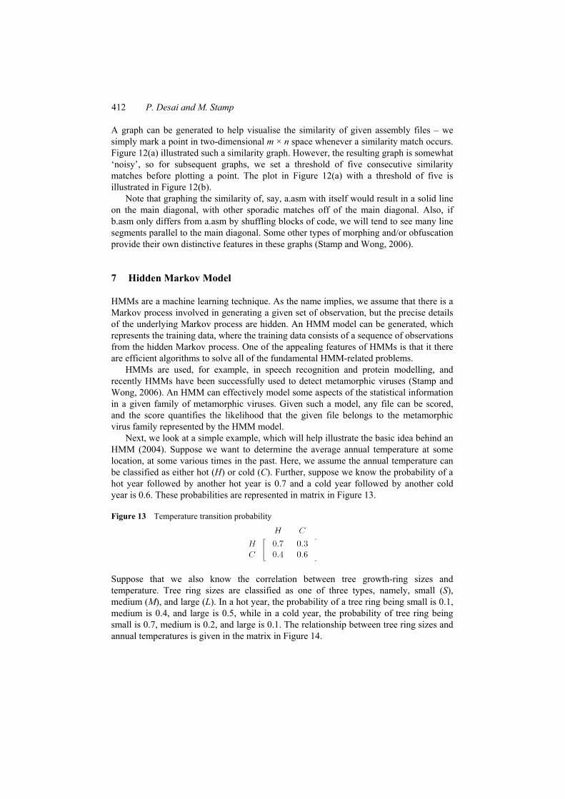
Next, we look at a simple example, which will help illustrate the basic idea behind an HMM (2004). Suppose we want to determine the average annual temperature at some location, at some various times in the past. Here, we assume the annual temperature can be classified as either hot (H) or cold (C). Further, suppose we know the probability of a hot year followed by another hot year is 0.7 and a cold year followed by another cold year is 0.6. These probabilities are represented in matrix in Figure 13.
Figure 13 Temperature transition probability
Suppose that we also know the correlation between tree growth-ring sizes and temperature. Tree ring sizes are classified as one of three types, namely, small (S), medium (M), and large (L). In a hot year, the probability of a tree ring being small is 0.1, medium is 0.4, and large is 0.5, while in a cold year, the probability of tree ring being small is 0.7, medium is 0.2, and large is 0.1. The relationship between tree ring sizes and annual temperatures is given in the matrix in Figure 14.

A highly metamorphic virus generator 413
Figure 14 Tree size probability
In this example, the annual temperatures are the ‘states’ of the (hidden) Markov process, while the tree ring sizes are the observations. The probability of the various tree ring sizes at each temperature represents the probability of the observation symbols in each state.
To summarise, the states (H and C) are hidden, since we cannot directly observe the temperature at some time in the past, and these hidden states are driven by a Markov process, as given by the matrix in Figure 13. In addition, we can observation tree ring sizes (S, M, and L) over a series of years. Apparently, there is a statistically relationship between the observations (tree ring size) and the hidden states (annual temperature). In this example, we would like to recover information about the hidden states from the observations.
Now suppose that we obtain the following sequence of observation symbols: (S, M, S, L). Note that this represents tree ring sizes for four consecutive years. We want to determine the most likely sequence of states (average annual temperature) for each of these four years, based on the given sequence of tree ring sizes.
Before we can solve this problem, we need some notation. The following notation is fairly standard with HMMs:
{ }0 1 1
mod
, , ,
T
T length of the observed sequenceN number of states in the elM number of distinct observation symbolsO observation sequence O O OA state transition probability matrixB observation probabilit
−
===
=
==
K
y distribution matrixinitial state distribution matrixπ =
In this example, the matrix A appears in Figure 14, and we have N = 2. The observation probability distribution matrix B, is the matrix in Figure 13 and we see that M = 3. That is, we have the following:
0.7 0.30.4 0.6
and0.1 0.4 0.50.7 0.2 0.1
A
B
⎡ ⎤= ⎢ ⎥⎣ ⎦
⎡ ⎤= ⎢ ⎥⎣ ⎦
The A and B matrix probabilities are related as illustrated in the Figure 15. The initial state distribution matrix, π represents the probability of being in a state
initially. Suppose that the initial state distribution matrix for this example is known to be
[0.6 0.4]π =

414 P. Desai and M. Stamp
The matrices A, B, and π define the HMM. Note that A, B, and π are row stochastic matrices, that is, each row is a probability distribution.
Figure 15 HMM model
Now we are ready to consider our given observation sequence, (S, M, S, L), which is of length T = 4. To determine the most probable state transitions for this sequence, we could use the following brute force approach:
1 Determine all of the NT possible state transitions.
2 Calculate the probability of the given observation sequence for each state transition obtained in Step 1. For example, to compute the probability of the state sequence HHCC, we have:
, , ,( ) * ( )* * ( )* * ( )* * ( )
(0.6)*(0.1)*(0.7)*(0.4)*(0.3)*(0.7)*(0.6)*(0.1)0.000212
H H H H H H C C C C CP HHCC b S a b M a b S a b Lπ=
==
3 The state sequence with highest probability is selected.
Figure 16 lists the probabilities of observing (S, M, S, L) for each of the 16 possible state sequences. We conclude that for the given sequence of observations, the most probable state sequence is CCCH. That is, given the observed tree ring sizes, the most likely scenario for the four-year period under consideration is that that there were three cold years followed by one hot year.
The real strength of the HMM approach is that we can derive an efficiently algorithm for determining this probability, as opposed to using an exponential brute-force approach.
In addition, there are efficient algorithms to ‘train’ the HMM model given a sequence of observations. That is, we can use an efficient iterative process to determine the model, A, B, and π, given a sequence of observations. The only free parameter that we need to specify in advance is N, the dimension of the A matrix. This is the sense that an HMM is a machine learning technique – it ‘learns’ from the observation sequence, with virtually no input required from the user.

A highly metamorphic virus generator 415
Figure 16 Probabilities of observing (S, M, S, L) for all possible state sequences
There is a third problem that can be solved using HMMs. If we are given a model and a sequence of observations, we can use the model to efficiently assign a probability to the observation sequence. This probability represents the likelihood that the given sequence was generated by the same (hidden) Markov process that the model represents. For computational reasons, it is necessary to use log odds instead of computing actual probabilities, so the closer the resulting ‘score’ is used to determine whether the observations match the model or not. With proper testing, a sensible threshold score can be determined.
7.1 HMM as virus detection tool
Using HMMs as a virus detection tool requires a sequence of observations that can be used as training data to generate a model. For training data, we follow (Stamp and Wong, 2006) and extract the opcodes from a ‘family’ of metamorphic viruses, where the family viruses all share the same functionality. We assume that we can obtain a number of such family viruses and we then disassemble each and extract the opcodes. The resulting sequences of opcodes are concatenated to yield our training data. The initial part of an observation sequence appears in Figure 17 with (part of) the resulting model given in Figure 18.
Once the model has been constructed, we can test it on family viruses that were not used to construct the model, as well as on ‘normal’ files. Using the resulting scores, we can set a threshold for scoring unknown files.
When given a file to test against the HMM model, we first disassemble the file and extract its sequence of opcodes. This sequence is then scored against the model that we previously constructed and the predetermined threshold is used to categorise the file as either a ‘family virus’ or ‘other’. We will present several examples of scoring results in Section 9, below.
For much more on HMMs, including pseudo-code for each of the three problems discussed here (see HMM, 2004).

416 P. Desai and M. Stamp
Figure 17 Training data, (a) unique symbols (b) observation sequence (see online version for colours)
(a) (b)
Figure 18 HMM model (see online version for colours)

A highly metamorphic virus generator 417
8 Implementation
8.1 Introduction
Our metamorphic generator is inspired, to an extent, by the Evol virus. Evol uses code morphing techniques such as dead code insertion, register/operands usage exchange, and equivalent instruction substitution. However, our approach includes more metamorphic techniques than Evol. The remainder of this section gives a fairly detailed explanation of our metamorphic engine.
Our implementation aimed to achieve the following goals:
• Generate morphed copies of a single input virus. These morphed copies should have minimum similarity with the base virus and among themselves, as measured by the similarity index discussed in Section 6.
• The morphed copies should have the same functionality as the base virus.
• A morphed copy should be as close (in terms of similarity) to ‘normal’ code as possible. For our examples of normal programmes, we rely on a set of cygwin utility files, which are each about the same size as the base virus. The reason we chose these ‘normal’ files is because they are probably doing somewhat similar low-level operations that we might expect from a virus.
• The metamorphic engine should work with any functioning assembly programme as input.
8.2 Code obfuscation techniques
8.2.1 Dead code insertion
Our dead code insertion consists of adding NOPs or other do-noting instructions. We also use dead code insertion to introduce opcodes that are not present or uncommon in the base virus.
Figure 19 Base virus opcodes and their frequency (see online version for colours)

418 P. Desai and M. Stamp
We first generate opcode statistics of the given base virus. The graph in Figure 19 lists the opcodes used in a particular base virus along with their relative frequencies.
The base virus in Figure 19 has 27 unique opcodes and six of them appear more than ten times. The most common opcodes are mov, push, add, call, cmp, and jz.
We then computed opcode frequencies for normal programmes. The graph in Figure 20 shows typical statistics.
Figure 20 Opcodes of normal file and their frequency (see online version for colours)
When the statistics of the normal file is compared with the base virus, we obtain the following list of opcodes that are unique to a normal file: and, int, fnstcw, or, fldcw, leave, jns, setnz, setz, jb, cld, jnb, shl, inc, fld, fstp, and repe.
These unique opcodes are included in our dead code insertion so as to make the morphed code look, in a statistical sense, somewhat more normal than the original virus. Figure 21 shows some examples of dead code instructions generated by our metamorphic generator for this example.
Figure 21 Arithmetic dead code instructions
1 add R, 0 2 sub R, 0 3 adc bx, 0 4 sbb bx, 0 5 inc R followed by dec R
The dead code instructions in Figure 21 are injected at randomly selected locations in the base virus.
We also introduced a simple unconditional jump NOP instruction. The jump NOP works by placing an unconditional jump to the next immediate instruction. An example of this variation is shown below.

A highly metamorphic virus generator 419
, [ int] 010235
010235 : , [ int]
Mov edx esi entryPojmp plplmov edx esi entryPo
+
+
8.2.1.1 Dead code sequences
In addition to inserting single instruction dead code, we also inserted dead code sequences. As above, the insertion location and the dead code sequences are selected randomly.
8.2.1.2 Transformations used in Evol
Along with dead code insertion, we introduced several Evol-inspired transformations (OpenRCE, 2002). The Evol virus substitutes a single instruction by surrounding it with dead code. Some of the specific Evol transformations we used are listed in Figure 22.
Figure 22 Evol transformations

420 P. Desai and M. Stamp
One disadvantage to these transformations is that we substitute a block of instructions for a single instruction. The ‘push’ and ‘pop’ bounding of each block is also distinctive. Excessive use of these transformations would increase the number of push and pop opcodes and could conceivably lead to an effective heuristic for detecting the code produced by our metamorphic engine (ISCAS, 2007). However, we used these transformations relatively sparingly.
8.2.2 Equivalent code substitution
Opcodes such as mov, push, add, call, cmp, and jz appear frequently in the base virus. To adjust the frequencies of these common opcodes, we used equivalent instruction substitution. In an equivalent instruction substitution, an instruction is replaced with another instruction or a block of instructions with the same functionality. For example substitutions for add are listed in Figure 23.
Figure 23 Substitutions for add
add R, imm 1 sub R, new_imm where new_imm = imm x(–1) 2 lea R, [R + imm] add R, 1 1 not R 2 neg R
8.2.3 Transpose
We also apply transposition to morph the code. Our transpose algorithm is outlined below:
1 read two instructions with two operands
2 generate a random number between 0 and 3
3 if the random number is 0 then perform transpose
4 to perform transpose: a read third instruction b if the third instruction is not any conditional jump instruction then:
• if to-operands of both instructions are not equal and to-operand of first instruction is not equal to from-operand of second instruction and from-operand of first instruction is not equal to to-operand of second instruction: 1 swap two instructions.
The above transpose algorithm applies only to instructions with register operands. We extended this algorithm to include instructions with memory operands. To achieve this extension, we added another condition. While comparing the operands in both the instructions, we had to make sure that none of the registers are used as memory pointers. For example, the following two instructions can be swapped:
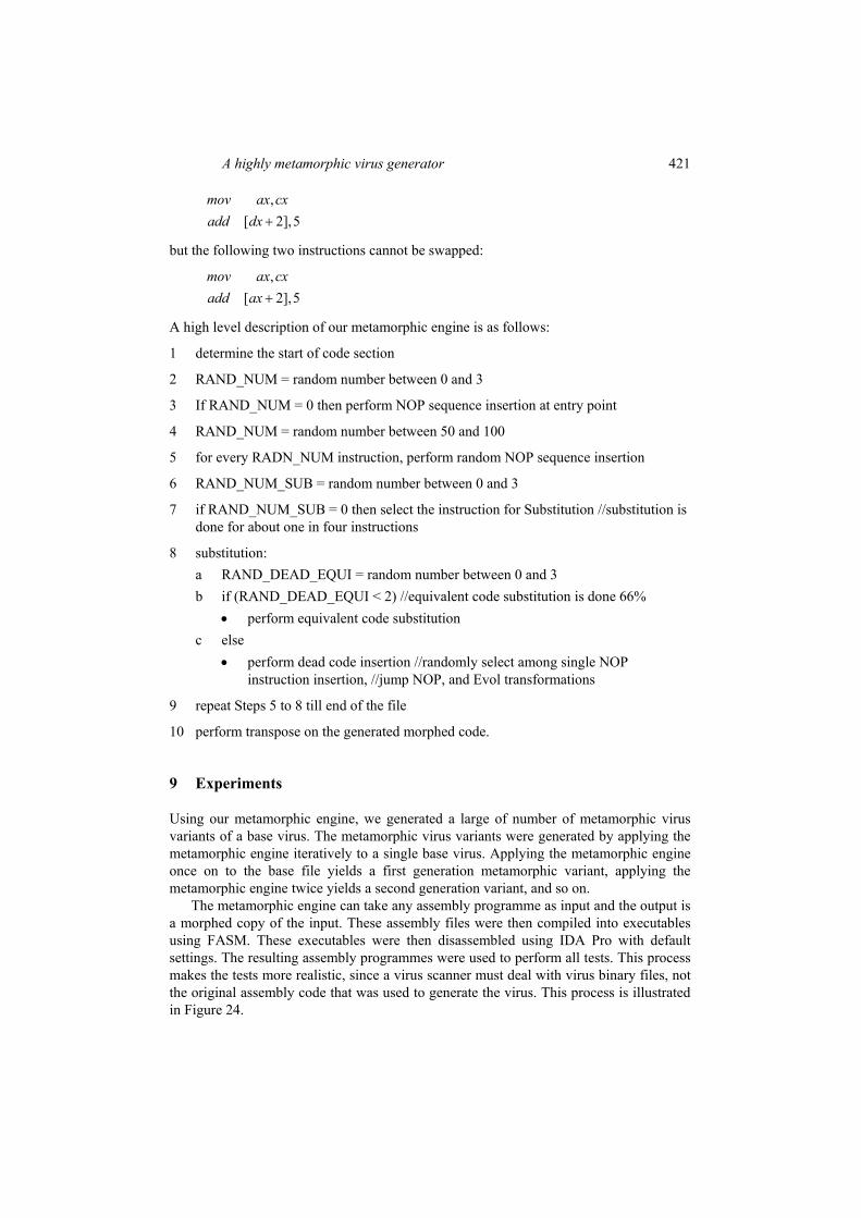
A highly metamorphic virus generator 421
,
[ 2],5mov ax cxadd dx +
but the following two instructions cannot be swapped:
,[ 2],5
mov ax cxadd ax +
A high level description of our metamorphic engine is as follows:
1 determine the start of code section
2 RAND_NUM = random number between 0 and 3
3 If RAND_NUM = 0 then perform NOP sequence insertion at entry point
4 RAND_NUM = random number between 50 and 100
5 for every RADN_NUM instruction, perform random NOP sequence insertion
6 RAND_NUM_SUB = random number between 0 and 3
7 if RAND_NUM_SUB = 0 then select the instruction for Substitution //substitution is done for about one in four instructions
8 substitution: a RAND_DEAD_EQUI = random number between 0 and 3 b if (RAND_DEAD_EQUI < 2) //equivalent code substitution is done 66%
• perform equivalent code substitution c else
• perform dead code insertion //randomly select among single NOP instruction insertion, //jump NOP, and Evol transformations
9 repeat Steps 5 to 8 till end of the file
10 perform transpose on the generated morphed code.
9 Experiments
Using our metamorphic engine, we generated a large of number of metamorphic virus variants of a base virus. The metamorphic virus variants were generated by applying the metamorphic engine iteratively to a single base virus. Applying the metamorphic engine once on to the base file yields a first generation metamorphic variant, applying the metamorphic engine twice yields a second generation variant, and so on.
The metamorphic engine can take any assembly programme as input and the output is a morphed copy of the input. These assembly files were then compiled into executables using FASM. These executables were then disassembled using IDA Pro with default settings. The resulting assembly programmes were used to perform all tests. This process makes the tests more realistic, since a virus scanner must deal with virus binary files, not the original assembly code that was used to generate the virus. This process is illustrated in Figure 24.
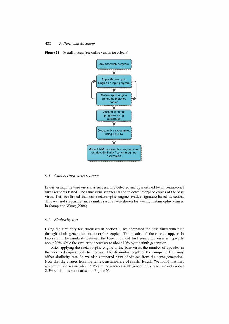
422 P. Desai and M. Stamp
Figure 24 Overall process (see online version for colours)
Any assembly program
Apply Metamorphic Engine on input program
Metamorphic engine generates Morphed
copies
Assemble output programs using
assembler
Disassemble executables using IDA-Pro
Model HMM on assembly programs and conduct Similarity Test on morphed
assemblies
9.1 Commercial virus scanner
In our testing, the base virus was successfully detected and quarantined by all commercial virus scanners tested. The same virus scanners failed to detect morphed copies of the base virus. This confirmed that our metamorphic engine evades signature-based detection. This was not surprising since similar results were shown for weakly metamorphic viruses in Stamp and Wong (2006).
9.2 Similarity test
Using the similarity test discussed in Section 6, we compared the base virus with first through ninth generation metamorphic copies. The results of these tests appear in Figure 25. The similarity between the base virus and first generation virus is typically about 70% while the similarity decreases to about 10% by the ninth generation.
After applying the metamorphic engine to the base virus, the number of opcodes in the morphed copies tends to increase. The dissimilar length of the compared files may affect similarity test. So we also compared pairs of viruses from the same generation. Note that the viruses from the same generation are of similar length. We found that first generation viruses are about 50% similar whereas ninth generation viruses are only about 2.5% similar, as summarised in Figure 26.

A highly metamorphic virus generator 423
Figure 25 Similarity results of the base virus v/s nine different generations (see online version for colours)
Figure 26 Similarity of two N generation viruses (see online version for colours)
In Stamp and Wong (2006), it was found that the next generation virus creation kit (NGVCK) produces the most highly metamorphic variants of any of the ‘hacker’ metamorphic engines tested. On average, NGVCK variants are about 10% similar (Stamp and Wong, 2006). Note that our ninth generation metamorphic variants are much more diverse than NGVCK viruses – the average similarity between our viruses is only about 2.5%, while the comparable number for NGVCK is about 10%. This shows that we achieved our goal of producing the most highly metamorphic virus variants yet seen.

424 P. Desai and M. Stamp
Next, we consider HMM-based detection, using our highly dissimilar ninth generation viruses. This would appear to provide a tremendous challenge for the HMM-based detection approach.
9.3 HMM-based detection
Next, we attempt to detect our morphed virus variants using the HMM-based detection methods from Stamp and Wong (2006).
9.3.1 A ninth generation virus model
We trained an HMM based on a set of 120 viruses, all of which were ninth generation metamorphic variants of a single base virus. The HMM model was developed using 90 of the viruses, with the 30 remaining viruses reserved for tested against the resulting model. This model used two hidden states. Stamp and Wong (2006) has shown that a larger number of hidden states does not significantly improve the model. Using the resulting model, scores for family viruses and normal files are given in Figure 27 and plotted in Figure 28.
Figure 27 Ninth generation HMM model
Ninth generation model with N =2
Family viruses Normal files G9_0 –3.1677 G9_15 –4.2650 N0 –14.4239 N15 –356.9657 G9_1 –3.164 G9_16 –3.1277 N1 –42.9527 N16 –34.4798 G9_2 –3.1269 G9_17 –3.1266 N2 –444.9695 N17 –11.7943 G9_3 –3.1419 G9_18 –3.1248 N3 –532.4239 N18 –406.5270 G9_4 –3.1596 G9_19 –3.1138 N4 –20.8160 N19 –406.5270 G9_5 –3.1692 G9_20 –3.1250 N5 –18.7624 N20 –507.2849 G9_6 –3.1419 G_21 –3.1486 N6 –20.8160 N21 –15.2849 G9_7 –3.1782 G9_22 –3.1517 N7 –17.2520 N22 –507.2849 G9_8 –3.1115 G9_23 –3.1661 N8 –27.8287 N23 –473.7664 G9_9 –3.1305 G9_24 –3.1420 N9 –19.0357 N24 –356.7943 G9_10 –3.1404 G9_25 –3.1743 N10 –406.5270 N25 –36.2016 G9_11 –3.1262 G9_26 –3.1522 N11 –37.8043 N26 –32.1237 G9_12 –3.1299 G9_27 –3.1638 N12 –25.4653 N27 –507.2849 G9_13 –3.1424 G9_28 –3.2038 N13 –23.9582 N28 –35.0315 G9_14 –3.1300 G9_29 –3.1714 N14 –25.2204 N29 –356.9657
Min score = –4.2650 Max score = –11.7943
Based on the results in Figure 27, we would like to set a threshold. Then any file scoring higher than this threshold is deemed a metamorphic virus variant of the type the model was trained to detect, and any file scoring lower is considered to not be such a virus. Using a threshold of, say, –0.6, we would have perfect detection, that is, the HMM would never make a mistake.

A highly metamorphic virus generator 425
Figure 28 Family viruses and normal files tested against ninth generation model (see online version for colours)
This result is surprising and clearly shows the strength of an HMM-based detection technique. Our ninth generation virus variants have virtually no similarity to each other, yet a properly trained HMM model is able to easily distinguish between these metamorphic viruses and normal files. Several more related experiments are discussed in Desai (2008).
10 Conclusions and future work
We developed a metamorphic engine that yields morphed copies of a given base assembly file. We showed that by using a known virus as our base file, and iterating this process over several generations, we can produce highly morphed and highly dissimilar virus files. These were among the main criteria suggested in Stamp and Wong (2006) as ways to defeat an HMM-based detection scheme. From this perspective, it appeared likely that these morphed viruses would successfully evade HMM-based detection.
Surprisingly, the HMM-based detector was still able to correctly classify viruses and normal files in every case tested. This shows that even with high metamorphism and virtually no similarity between the morphed viruses, an HMM is able to identify a common pattern in the morphed viruses. In short, the HMM has proved itself extremely robust and very difficult to defeat.
Perhaps, one area for improvement over our approach lies with dead code insertion and its effect on the file size. The size of the base virus we selected was 1.5 KB. Applying our metamorphic engine tends to increase the file size, and applying the engine over several generations increases the original file size significantly. The increase is size as a function of the number of iterations is illustrated in Figure 29.
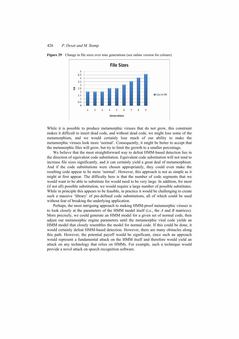
426 P. Desai and M. Stamp
Figure 29 Change in file sizes over nine generations (see online version for colours)
While it is possible to produce metamorphic viruses that do not grow, this constraint makes it difficult to insert dead code, and without dead code, we might lose some of the metamorphism, and we would certainly lose much of our ability to make the metamorphic viruses look more ‘normal’. Consequently, it might be better to accept that the metamorphic files will grow, but try to limit the growth to a smaller percentage.
We believe that the most straightforward way to defeat HMM-based detection lies in the direction of equivalent code substitution. Equivalent code substitution will not tend to increase file sizes significantly, and it can certainly yield a great deal of metamorphism. And if the code substitutions were chosen appropriately, they could even make the resulting code appear to be more ‘normal’. However, this approach is not as simple as it might at first appear. The difficulty here is that the number of code segments that we would want to be able to substitute for would need to be very large. In addition, for most (if not all) possible substitution, we would require a large number of possible substitutes. While in principle this appears to be feasible, in practice it would be challenging to create such a massive ‘library’ of pre-defined code substitutions, all of which could be used without fear of breaking the underlying application.
Perhaps, the most intriguing approach to making HMM-proof metamorphic viruses is to look closely at the parameters of the HMM model itself (i.e., the A and B matrices). More precisely, we could generate an HMM model for a given set of normal code, then adjust our metamorphic engine parameters until the metamorphic viral code yields an HMM model that closely resembles the model for normal code. If this could be done, it would certainly defeat HMM-based detection. However, there are many obstacles along this path. However, the potential payoff would be significant, since such an approach would represent a fundamental attack on the HMM itself and therefore would yield an attack on any technology that relies on HMMs. For example, such a technique would provide a novel attack on speech recognition software.

A highly metamorphic virus generator 427
References Attaluri, S., McGhee, S. and Stamp, M. (2008) ‘Profile hidden Markov models and metamorphic
virus detection’, Journal in Computer Virology, Vol. 5, No. 2, pp.151–169. Aycock, J. (2006) Computer Viruses and Malware, Springer. Borello, J. and Me, L. (2008) ‘Code obfuscation techniques for metamorphic viruses’, Journal in
Computer Virology, Vol. 4, No. 3, pp.211–220. Chouchane, M., Lakhotia, A., Mathur, R. and Walenstein, A. (2007) ‘The design space of
metamorphic malware’, Paper presented at the Proceedings of the 2nd International Conference on Information Warfare, 8–9 March, California, USA.
Daoud, E. and Jebril, I. (2008) ‘Computer virus strategies and detection methods’, Int. J. Open Problems Compt. Math., Vol. 1, No. 2, pp.29–36.
Desai, P. (2008) ‘Towards an undetectable computer virus’, Masters report, San Jose State University, USA.
HMM (2004) A Revealing Introduction to Hidden Markov Models, available at http://www.cs.sjsu.edu/faculty/stamp/RUA/HMM.pdf (accessed on 23 February 2008).
ISCAS (2007) Are Metamorphic Viruses Really Invincible?, available at http://www.iscas2007.org/~arun/papers/invincible-complete.pdf (accessed on 3 April 2008).
Mishra, P. (2003) ‘A taxonomy of software uniqueness transformations’, Masters report, San Jose State University, USA.
OpenRCE (2006) ‘The viral Darwinism of W32.Evol: an in-depth analysis of a metamorphic engine’, available at http://www.antilife.org/files/Evol.pdf (accessed on 23 February 2008).
Stamp, M. (2005) Information Security: Principles and Practice, Wiley. Stamp, M. and Wong, W. (2006) ‘Hunting for metamorphic engines’, Journal in Computer
Virology, Vol. 2, No. 3, pp.211–229. Szor, P. (2005) The Art of Computer Virus Defense and Research, Symantec Press. VXHEAVENS (1999) Theme: Metamorphism, available at
http://www.vx.netlux.org/lib/static/vdat/ep metam2.htm (accessed on 3 March 2008). VXHEAVENS (2002) How I Made MetaPHOR and What I’ve Learnt, available at
http://vx.netlux.org/lib/vmd01.html (accessed on 5 March 2008).

![Hunting for metamorphic engines - Ptolemy Project...Hunting for metamorphic engines 213 Fig. 1 Shapes of a metamorphic virus [24] n! different viruses.W32/Ghost has ten subroutines,](https://static.fdocuments.us/doc/165x107/5f990ab0f1bb5023eb347191/hunting-for-metamorphic-engines-ptolemy-project-hunting-for-metamorphic-engines.jpg)


![Chi-Squared Distance and Metamorphic Virus Detection · A virus is often de ned as malware that relies on passive propagation, whereas a worm uses active means [21]. That is, a worm](https://static.fdocuments.us/doc/165x107/5f03de4a7e708231d40b29c7/chi-squared-distance-and-metamorphic-virus-a-virus-is-often-de-ned-as-malware-that.jpg)