m

NASA Contractor Report 201674

/is f,,.... <_5°_:;9/

A Higher-Order Bending Theory forLaminated Composite and SandwichBeams

Geoffrey M. Cook

George Washington UniversityJoint Institute for Advancement of Flight Sciences

Hampton, Virginia

Cooperative Agreement NCC1-208

March 1997

National Aeronautics and

Space Administration

Langley Research Center

Hampton, Virginia 23681-000i

https://ntrs.nasa.gov/search.jsp?R=19970015285 2018-05-21T13:36:39+00:00Z

Abstract

A higher-order bending theory is derived for laminated composite and sandwich beams.

The recent { 1,2}-order theory is extended to include higher-order axial effects without

introducing additional kinematic variables. This is accomplished by assuming a special

form for the axial and transverse displacement expansions. An independent expansion is

also assumed for the transverse normal stress, improving the transverse strain and stress

predictive capability of the theory. Appropriate shear correction factors based on energy

considerations are used to adjust the shear stiffness, thereby improving the transverse

displacement response. A set of transverse normal correction factors is introduced,

leading to significant improvements in the transverse normal strain and stress for

laminated composite and sandwich beams. A closed-form solution to the cylindrical

bending problem is derived, demonstrating excellent correlation to the corresponding exact

elasticity solutions for a wide range of beam aspect ratios and commonly used material

systems. Accurate shear stresses for a wide range of laminates, including the challenging

unsymmetric composite and sandwich laminates, are obtained using an original corrected

integration scheme. For application of the theory to a wider range of problems, guidelines

for finite element approximations are presented.

Table of Contents

Abstract ................................................................................................................................ i

List of Figures ...................................................................................................................... iv

List of Tables ....................................................................................................................... iv

Nomenclature ....................................................................................................................... v

1. Introduction ...................................................................................................................... 1

2. Mathematical Formulation ................................................................................................ 6

2.1 Higher-Order Theory for Laminated Beams ............................................................ 7

2.1.1 Kinematic Displacement Assumptions .......................................................... 8

2.1.2 Reduced Stress-Strain Relations .................................................................... 12.

2.1.3 Strain-Displacement Relations .................................................................... 12

2.1.4 Variational Principle ................................................................................... 17

2.1.5 Equilibrium Equations and Boundary Conditions .......................................... 19

2.1.6 Beam Constitutive Relations ....................................................................... 20

2.1.7 Equilibrium Equations in Terms of Displacements ....................................... 20

2.2 Reduction of Present Theory to Lower-Order Theories ........................................ 22

3. Adjustments to Theory ................................................................................................... 23

3.1 Shear Correction Factors ...................................................................................... 23

3.2 Transverse Correction Factors .............................................................................. 25

3.3 Integrated Interlaminar Shear Stress ...................................................................... 28

4. Cylindrical Bending Problem ........................................................................................... 34

4.1 Closed-Form Solution ........................................................................................... 34

4.2 Material Properties ............................................................................................... 36

4.3 Test Case Definition ............... :............................................................................. 37

4.4 Correction Factors ................................................................................................ 38

4.5 Results .................................................................................................................. 39

4.5.1 Homogeneous Beams .................................................................................. 41

4.5.2 Laminated Composite Beams ............................................. _................ _....... 45

4.5.3 Sandwich Beams .......................................................................................... 52

5. Guidelines for Finite Element Approximations ................................................................ 63

6. Conclusions and Recommendations ................................................................................. 66

REFERENCES .................................................................................................................... 68

Appendix A: Transverse Normal Strain Coefficients ........................................................... 71

Appendix B: Stress Resultants and Prescribed Tractions ...................................................... 73

Appendix C: Stiffness Coefficients for Beam Constitutive Matrix ....................................... 74

Appendix D: Derivation of Constitutive Relations .............................................................. 76

.°.

111

Figure 2.1

Figure 3.1

Figure 3.2

Figure 3.3

Figure 3.4

Figure 4.1

Figure 4.2

Figure 4.3

Figure 4.4

Figure 4.5

Figure 4.6

Figure 4.7

Figure 4.8

Figure 4.9

Figure 4.10

Figure 4.11

Figure 4.12

Figure 4.13

Figure 4.14

Figure 4.15

Figure 4.16

Figure 4.17

Figure 4.18

Figure 4.19

Figure 4.20

Figure 4.21

Figure 5.1

List of Figures

Sign Convention for Beam .............................................................................. 7

Transverse Correction for a Sandwich Beam ...................... . .................... i.... 28

Comparison of Shear Stress and Strain for an Unsymmetric Laminate ........ 29

Integration Errors Caused by Stretching of the Midplane ............................ 30

Error Function and Lamination Notation ..................................................... 32

Cylindrical Bending Problem ........................................................................ 34

Locations for Displacement, Strain, and Stress Computations .................... 40

Case A: Aluminum, L/2h = 100 .................................................................... 42

Case A: Aluminum, L/2h = 10 ...................................................................... 43

Case A: Aluminum, L/2h = 4 ........................................................................ 44

Case B: Gr/Ep Symmetric Laminate, L/2h = 100 ......................................... 46

Case B: Gr/Ep Symmetric Laminate, L/2h = 10 ........................................... 47

Case B: Gr/Ep Symmetric Laminate, L/2h = 4 .................................. , .......... 48

Case C: Gr/Ep Unsymmetric Laminate, L/2h = 100 .................................... 49

Case C: Gr/Ep Unsymmetric Laminate, L/2h = 10 ...................................... 50

Case C: Gr/Ep Unsymmetric Laminate, L/2h = 4 ........................................ 51

Sandwich Composite Beam .......................................................................... 52

Case D: Gr/Ep-PVC Symmetric Sandwich, L/2h = 100 ............................... 54

Case D: Gr/Ep-PVC Symmetric Sandwich, L/2h = 10 ................................. 55

Case D: Gr/Ep-PVC Symmetric Sandwich, L/2h = 4 ................................... 56

Case E: Gr/Ep-Ti Symmetric Sandwich, L/2h = 100 .................................... 57

Case E: Gr/Ep-Ti Symmetric Sandwich, L/2h = 10 ........................ .............. 58

Case E: Gr/Ep-Ti Symmetric Sandwich, L/2h = 4 ........................................ 59

Case F: Gr/Ep-PVC Unsymmetric Sandwich, L/2h = 100 ........................... 60

Case F: Gr/Ep-PVC Unsymmetric Sandwich, L/2h = 10 ............................. 61

Case F: Gr/Ep-PVC Unsymmetric Sandwich, L/2h = 4 ............................... 62

Finite Element Model of a Tapered Beam .................................................... 65

List of Tables

Table 4.1

Table 4.2

Table 4.3

Table 4.4

Material Properties .......................................................................................... 37

Definition of Test Cases and Corresponding Ply Layup ................................ 38

{3,2} Theory Correction Factors .................................................................... 39

{ 1,2} Theory Correction Factors .................................................................... 39

iv

A

Aij

b

Bij

C_ k)

Dij

Fk

G

Gij

2h

hk, hk_l

k

(k)

kzo, kzl

L

M

Mx, Mz, MH

Mio, M_.

N

Nx, Nz, NH

xo, N'x

Pi, ri, Pi, Ri

q+, q-

Qx

Qio, Qm

S+,S"

s}jtk

Txo, TxL, Tzo,

TzL

Nomenclature

cross-sectional area of beam

membrane beam rigidities

beam width

membrane-bending coupling beam rigidities

elastic stiffness coefficients for k th ply

bending beam rigidities

Young's moduli

Heaviside unit function for k th ply

shear rigidity

shear moduli

beam thickness

distances from midplane to bottom and top surfaces k th of ply

sheax correction factor

ply index for laminate

transverse correction factors

beam span

number of 0 ° plies in laminate

axial, transverse, and higher-order bending moment resultants

prescribed end moment resultants

number of plies in laminate

axial, transverse, and higher-order membrane force resultants

prescribed end force resultants

constants for transverse normal strain thickness distributions

normal pressure loads on the top and bottom surfaces of beam

transverse shear force resultant

prescribed end shear force resultants

top and bottom surfaces of beam

elastic compliance coefficients for k th ply

thickness of k th ply

arbitrary stress components prescribed at ends of beam

[% ],U

Ux, Uz

UO_ Ub U2, U3

Ushear

W_ W b W 2

(X

8

F--,xx

_zz

Ex0_ EzO _E H

?

3rx_

3tx_O

KxO_ ]_zO_ KH

Vij

0

O'xx

(_zz

(_zn

"_xz

_k

_!k)1

stress and strain transformation matrices

midplane displacement along x-axis

axial and transverse displacement components

coefficients for axial displacement expansion

shear strain energy per unit length

transverse displacement components

tracer for shear stress error correction

orientation of principle material axis within each ply

variational operator

axial strain

transverse normal strain

axial, transverse, and higher-order strain measures

through the thickness distribution functions

shear angle

transverse shear strain

shear strain measure

axial, transverse, and higher-order curvatures

Poisson ratios

rotation of normal about y-axis

axial stress

transverse normal stress

coefficients for transverse normal stress expansion

transverse shear stress

shear stress error function for k th ply

transverse normal strain thickness distributions for k th ply

dimensionsless thickness coordinate

vi

1. Introduction

The high performance aircraft and spacecraft currently being considered for the next

generation of aerospace vehicles require the use of strong yet lightweight materials.

Laminated composites, such as graphite fiber reinforced epoxy, are commonly used for

spacecraft and aircraft where weight is critical. While composite laminates provide higher

stiffness, strength, and reduce weight over conventional metallic structures, sandwich

structures can further reduce the structural weight and improve thermal performance

without sacrificing stiffness and strength. A sandwich structure typically consists of two

laminated composite or metallic face sheets with a core of foam, metallic honeycomb, or

other lightweight material. The face sheets provide axial stiffness while the core acts as a

shear web to carry the transverse shear load. Core materials are typically lighter and

several orders of magnitude more compliant than the face sheet materials. This presents

an analytical challenge with respect to the prediction of strain and stress distributions

through the thickness. The knowledge of accurate, detailed strains and stresses is critical

to the design of lightweight aerospace structures. Without accurate strain and stress

predictions, higher factors of safety are often used, thereby increasing the weight and cost

while reducing performance.

Numerous bending theories to analyze the response of beam, plate, and shell structures

have been proposed. Many of the significant developments in elastic theory are

summarized in review papers by Reissner (1985), Reddy (1989), and Noor and Burton

(1989). The following discussion reviews the most pertinent developments in beam

theory, and also makes comparisons to similar plate and shell theories.

Classical Bernoulli-Euler beam theory is the earliest and simplest approximation used

for analysis of homogeneous beams. It dates back to 1705 and precedes the theory of

elasticity by over 100 years (Love, 1952). In the classical bending theory of beams, the

beam cross section is assumed to be much smaller than the length of the beam and the

displacements are small compared to the thickness of the beam. The transverse normal

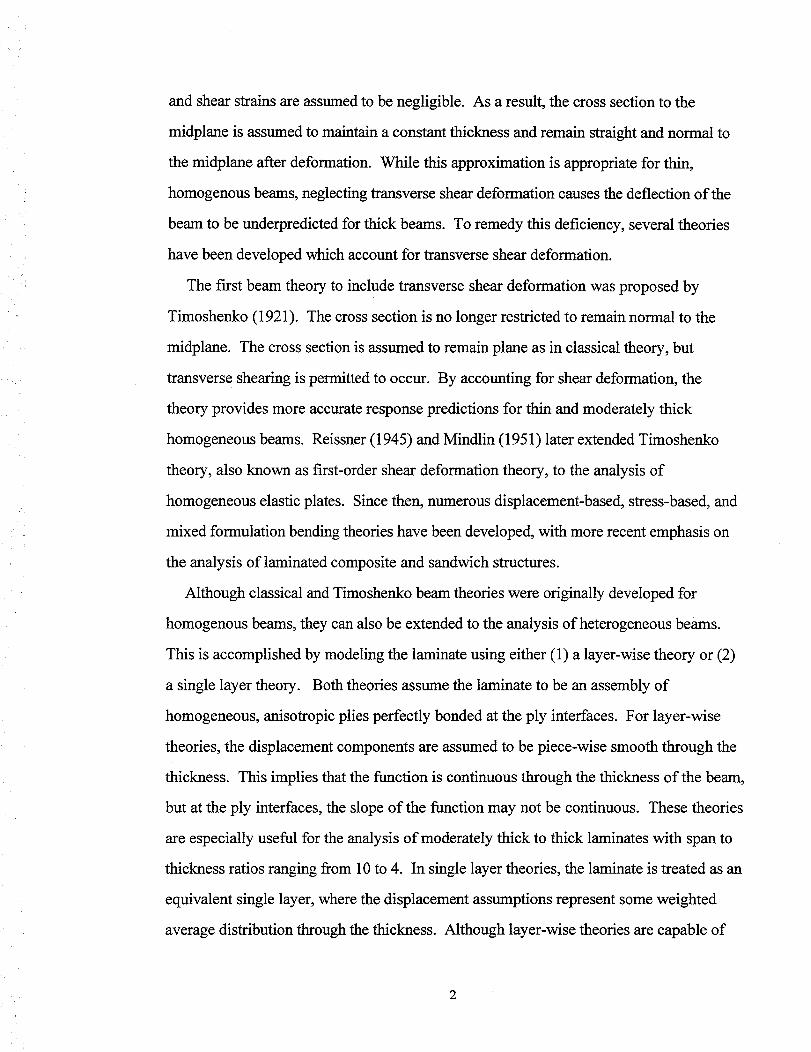
andshearstrainsareassumedto benegligible. As aresult,thecrosssectionto the

midplaneis assumedto maintainaconstantthicknessandremainstraightandnormal to

themidplaneafterdeformation.While this approximationis appropriatefor thin,

homogenousbeams,neglectingtransversesheardeformationcausesthedeflectionof the

beamto beunderpredictedfor thick beams.To remedythis deficiency,severaltheories

havebeendevelopedwhichaccountfor transversesheardeformation.

Thefirst beamtheoryto includetransversesheardeformationwasproposedby

Timoshenko(1921). Thecrosssectionis no longerrestrictedto remainnormalto the

midplane. Thecrosssectionis assumedto remainplaneasin classicaltheory,but

transverse shearingispermittedto occur. By accountingfor sheardeformation,the

theoryprovidesmoreaccurateresponsepredictionsfor thin andmoderatelythick

homogeneousbeams.Reissner(1945)andMindlin (1951)laterextendedTimoshenko

theory,alsoknown asfirst-ordersheardeformationtheory,to the analysisof

homogeneouselasticplates. Sincethen,numerousdisplacement-based,stress-based,and

mixedformulationbendingtheorieshavebeendeveloped,with morerecentemphasison

theanalysisof laminatedcompositeandsandwichstructures.

AlthoughclassicalandTimoshenkobeamtheorieswereoriginallydevelopedfor

homogenousbeams,theycanalsobeextendedto theanalysisof heterogeneousbeams.

This is accomplishedby modelingthelaminateusingeither(1) a layer-wisetheoryor (2)

asinglelayertheory. Boththeoriesassumethe laminateto beanassemblyof

homogeneous,anisotropicpliesperfectlybondedatthe ply interfaces.For layer-wise

theories,the displacementcomponentsareassumedto bepiece-wisesmooththroughthe

thickness.This impliesthatthefimction is continuousthroughthethicknessof the beam,

but at theply interfaces,theslopeof the functionmaynot becontinuous.Thesetheories

areespeciallyusefulfor theanalysisof moderatelythick to thick laminateswith spanto

thicknessratiosrangingfrom 10to 4. In singlelayertheories,thelaminateis treatedasan

equivalentsinglelayer,wherethedisplacementassumptionsrepresentsomeweighted

averagedistributionthroughthethickness.Although layer-wisetheoriesarecapableof

accuratemodelingof laminatedcompositesandsandwiches,thenumberof independent

variablesis directly proportionalto thenumberof plies in the laminate. Solutions to

these equations can become computationally expensive and intractable as the number of

layers in the laminate increases (Reddy and Liu,1987). The single layer theories are found

to be the most computationally efficient and will provide the background for the present

higher-order theory.

For single layer, displacement-based theories, the displacement approximations are

assumed to take on a particular polynomial form through the laminate thickness. Each

term in the expansion adds an additional power of the thickness coordinate, while the

expansion coefficients are functions of the x coordinate only. These approximations are

the basis for the development of the strain and stress quantities, and hence will govern the

complexity and accuracy of the theory. The axial displacements are expanded with a

polynomial of degree, m, while the transverse displacement may be of a different degree,

n. Thus, the notation {m,n} may be used to distinguish between the different order single

layer theories (Tessler and Saether, 1991).

One of the most commonly used approximations for single layer displacement-based

theories is { 1,0}(or first-order) shear deformation theory, i.e., having a linear axial

displacement and a constant transverse displacement. With the advent of advanced

composite materials, there has been a great deal of work in the development of plate •

theories which extend the Timoshenko beam theory and Reissner-Mindlin plate theory to

the analysis of laminated, heterogeneous structures. Stavsky (1959) is apparently the

first to develop such a theory, and improvements upon this theory have been made by

Yang, et al. (1966) and Whitney and Pagano (1970). Even with modifications to the

theory, the detailed stress distributions show little improvement over the classical theory

for moderately thick heterogeneous beams. Although the transverse shear stresses are

included in these theories, the transverse normal stresses are neglected. Both transverse

shear and transverse normal stresses become significant for moderately thick to thick

laminated composite and sandwich beams. They often contribute to delaminations of the

•

plies and subsequent structural failure. Thick composites and sandwiches generally

exhibit nonlinear displacement and strain distributions through the thickness which cannot

be predicted using linear displacement assumptions. Because of the inadequacies of the

first-order shear deformation theories, higher-order theories have been developed which

attempt to predict more accurately the response of heterogeneous structures.

Higher-order theories in this context refer to the class of theories, for either beams,

plates, or shells, in which the polynomial expansions of the displacement field are of

higher order than { 1,0} approximations. While the { 1,0} Timoshenko beam theory

includes transverse shear deformation, the transverse normal strains are still assumed

negligible. Essenburg (1975) proposed a { 1,2}-order beam theory which includes

transverse normal effects, and a similar plate theory has been proposed by Whitney and

Sun (1974). Lo, et al. (1977) developed a {3,2} laminated plate theory which produces

adequate predictions for inplane displacement and stress distributions. The theory has a

higher degree of complexity having eleven kinematic variables, and its predictive

capability for the transverse normal and shear stresses is rather poor.

As a compromise between accuracy and computational efficiency, Reddy (1984)

developed a {3,0}-order theory. By taking a special form for the inplane displacement

components, the theory contains the same number of kinematic variables as the first-

order shear deformation theory. This special displacement form also results in the

parabolic distribution of the shear strain through the thickness. The shear stresses satisfy

the traction-free boundary conditions on the surfaces of the plate, an important physical

condition which previous theories did not enforce. Phan and Reddy (1985) investigated

solutions to the aforementioned theory, showing improvements over classical theory.

Tessler and coworkers (1991-1995) developed a { 1,2 }-order theory for beam, plate,

and shell analyses. The theory assumes a special form for the transverse displacement to

obtain the 'average', parabolic shear strain distribution and shear traction free surface

conditions. The theory is novel in that the transverse strains are not directly derived from

the strain-displacement relations. The transverse normal and shear strains are assumed as

4

independentpolynomialexpansions.Theyarerequiredto beleastsquarescompatible,

throughthelaminatethickness,to thestrainsobtaineddirectly from the strain-

displacementrelations.Theresultingthicknessdistributionsfor thetransversestresses

andstrainsshowadequatecorrelationwith resultsgivenby elasticitytheory,an

improvementoverprevioushigher-ordertheories. Tessler(1993a)improvedthetheory

further for applicationto compositesby introducingan independentpolynomial

assumptionfor thetransversenormalstressin placeof thetransversenormalstrain. The

improvedtheoryresultsin a moreaccuraterepresentationof transversenormalstresses

andstrains,andis furthersubstantiatedby solutionsgivenby Schleicher(1994). The

{ 1,2} theoryretainsthesimplicity of thefirst-ordersheardeformationtheoryasfar as

the engineeringboundaryconditionsareconcerned.Furthermore,thetheorygivesriseto

finite elementformulationsthatarecompatiblewith thefirst-ordersheardeformation

elements.

Applicationof the { 1,2} theorygenerallyresultsin excellentpredictionsfor thin and

moderatelythick homogeneousandlaminatedbeams,but thetheoryhassomedeficiencies

in modelingtheresponseof sandwichbeams.Thelinearaxialdisplacementassumption

cannotmodelthenonlinearthicknessdistributionsof theaxialdisplacementandstrain. In

thick laminates,thisgenerallyresultsin underestimationof theaxial stress,typically the

largeststresswhich governsthedesignof the structure.Theotherdeficiencyis the

transversenormalstressviolation of tractionconditionson thetop andbottomsurfaces

of sandwichbeams.

Themain objectiveof this reportis to expanduponTessler's{1,2} theoryby

proposingahigher-ordertheoryof order{3,2} which includesnonlinearaxialeffects. The

theoryis expectedto modelaccuratelythenonlinearaxialdisplacementandstrainthrough

thethicknessof thebeam,resultingin amoreaccurateaxial stressprediction. A special

form for thecubicaxial displacementfield is usedsuchthatnoadditionalkinematic

variablesareintroducedinto thetheory. This enablesthepresenthigher-ordertheoryto

retainthe simplicity of the { 1,2} theorywhile improving predictionsof the axial response

5

of thebeam. Thetransversenormalstressandtransverseshearstresspredictive

capabilitywill alsobe improvedfor sandwichbeams.

In Section2, themathematicalformulationof ahigher-ordertheoryis presented.The

{3,2}-order displacementfield is assumed.Thesedisplacementapproximationsaccount

for the nonlinearvariationsof stressandstrainquantitiestypically presentin thick

compositeandsandwichstructures.As in the {1,2}-order theory,a specialform of the

quadratictransversedisplacementis assumed.An independentexpansionisalsoassumed

for thetransversenormalstress,asin Tessler(1993a).However,theshearstrainis

computeddirectly from thestrain-displacementrelations. Becauseof thespecialform for

theaxial displacementassumption,thetraction-freeshearstressboundaryconditionsare

satisfiedexactly. Theprincipleof virtual work is usedto derivetheequilibriumequations

andboundaryequationsfor thetheory. Thehierarchicalform of the {3,2}-order

displacementapproximationspermitsa straightforwardreductionto lower-orderbeam

theoriesof TesslerandTimoshenko.

In Section3, transverseshearandtransversenormalcorrectionfactorsaredetermined

from theenergyandtractionequilibriumconsiderations.Furthermore,accuratepiece-

wisesmoothshearstressesaredeterminedby integratingthetwo-dimensionalequilibrium

equationof elasticitytheory. A correctionprocedureis alsodevelopedto improvethe

accuracyof thisapproachfor unsymmetricandsandwichlaminates.

In Section4, ananalyticsolutionto thecylindricalbendingproblemispresented.

Numericalresultsarepresentedfor commonlyusedaerospacematerialsystems.

Comparisonsaremadeto the {1,2} theoryandthree-dimensionalelasticitysolutions. In

Section5, guidelinesfor fmite elementformulationandimplementationbasedon the {3,2}

theoryarepresented.Finally, Section6 presentsconclusionsandrecommendationsfor

futurework.

6

2. Mathematical Formulation

This section discusses the derivation of a higher-order bending theory for

heterogeneous beams. A displacement field of order {3,2} is assumed and the strains,

stresses, equilibrium equations, and boundary conditions are derived.

2.1 Higher-Order Theory for Laminated Beams

Consider a straight, linearly elastic beam laminated with N orthotropic plies subject to

the loading shown in Figure 2.1. The beam has a span L and a rectangular cross-section of

thickness 2h and width b. The orthotropic plies are stacked from the bottom face (z = -h)

such that the material properties, in general, are functions of the z coordinate. The

loadings q÷ and q- are stresses applied normal to the top and bottom faces of the beam

and may vary in the x coordinate. Ti0 and TiE ( i = x,z) are arbitrary stress components

prescribed at the ends of the beam.

Z,U Z+

_X,U X

Z

l-bq

Figure 2.1 Sign Convention for Beam

2.1.1 Kinematic Displacement Assumptions

The first step in developing a displacement-based theory is to introduce kinematic

assumptions for the displacements. These assumptions are made by first choosing a

polynomial form for the displacement components. For thick laminated composite and

sandwich beams, the displacement components are piece-wise smooth and nonlinear

through the thickness. This contrasts with the predominantly linear displacement

distributions for thin beams. To capture these higher-order deformation effects, a cubic

polynomial is assumed for the axial displacement u x and a quadratic distribution is

assumed for the transverse displacement u z , i.e.

Ux(K , Z) = UO (X)"_ Ul(X)_ "-I- U2(X ) _2 ..1_ U3(X ) _3

u (x,z) =w(x)+w,(x); +w:(x) (;2 +c)(2.1)

_ z [-1,1] is the dimensionless thickness coordinate such that _ = 0 defmeswhere _ - _

the midplane of the beam. The four u i coefficients in the axial displacement expression

are independent unknowns to be determined. The w i coefficients in the transverse

displacement are kinematic variables identical to those defined by Tessler (1991). The

constant C is included in the transverse displacement equation to allow w(x) to represent

a weighted average transverse displacement.

Three conventional kinematic variables are introduced and defined, as in Reissner

(1945), as weighted average quantities through the thickness, such that

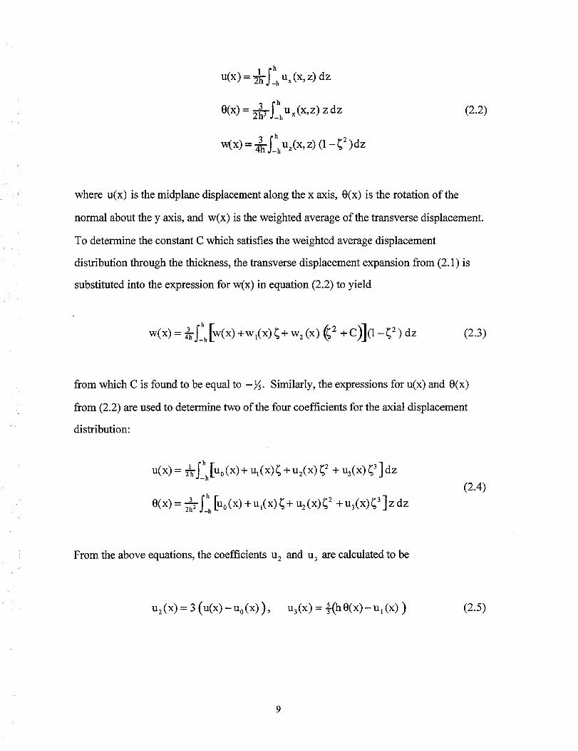
l h

u(x) = 7ri'Lh Ux(x, z) dz

3 trh

O(x) = 2-_J_hU_(X,Z) z dz

=

(2.2)

where u(x) is the midplane displacement along the x axis, 0(x) is the rotation of the

normal about the y axis, and w(x) is the weighted average of the transverse displacement.

To determine the constant C which satisfies the weighted average displacement

distribution through the thickness, the transverse displacement expansion from (2.1) is

substituted into the expression for w(x) in equation (2.2) to yield

3 hW(X) ----"_'_'f_h [W(X)q-Wl(X) _-I-W 2 (X)(_2 + C)](1 __z)dz (2.3)

from which C is found to be equal to -1/5. Similarly, the expressions for u(x) and 0(x)

from (2.2) are used to determine two of the four coefficients for the axial displacement

distribution:

1 h

U(X)= '_"_S_h [no (X)-[- Ul(X)_ -l" U2(X) _ 2 -I- U3(X) _3 ]dz

3 h

O(x)=_f_ [Uo(X)+u,(x);+ u_(x);_+u_(x)_]zdz(2.4)

From the above equations, the coefficients u 2 and u 3 are calculated to be

u:(x)=3(u(x)-uo(x)), u_(x)=÷(hO(x)-u,(x)) (2.5)

Theremainingcoefficientsaredeterminedby usingtheconditionthattheshearstressat

thetop andbottomfacesof thebeammustvanish,i.e. Zxz(X,z=+h)= 0. Becauseof the

directrelationshipbetweenstressandstrainin beamtheory, Zxz= C55_'x_,theshear

strainsat thetop andbottomfacesmustalsovanish:

r.(x, z=_+h)=O (2.6)

Using the strain-displacement relation for the transverse shear strain, Yxz = Ux,z + U_.x,

and equation (2.5) yields

(x,z) =6 (u(x) - u 0 (x)) z

W(X)-Jr. Ul (X) "1" WI(X)_Z ..} h2, h

/+ +w (x

(2.7)

where a comma.(,) denotes partial differentiation. After enforcing the two boundary

conditions from (2.6), the coefficients u o and u, are found to be

h wl(x), x h (25 0(x)+ 5 w(x) x + 4 w2(x), x )Uo(X) U(X)+ Ul (X) _-

6 ' 20(2.8)

Substitution of the coefficients u o, u,, u 2 , u 3, and the constant C into equation (2.1)

yields the final form of the displacement components:

Ux(X,Z) = u+ h;0-+(3 ;2_ 1 ) hw,,× -h; (_.;2_ _y

(2.9)

10 •

with theshearangle3' definedas

_(x) = _ [0(x)+ w x(X)]+W2,x(X) (2.1o)

The kinematic variables u, 0, w, Wl, and w 2 are functions of the x coordinate only.

Note that although the displacement assumptions in (2.1) contain seven independent

variables, the resulting displacements given in (2.9) are in terms of only five kinematic

variables, which are identical to those given in { 1,2}-order theory proposed by Tessler

(1991). The terms u(x), 0(x), and w(x) are the conventional Reissner variables defined

as weighted averages in equation (2.2). The higher-order terms for the transverse

displacement, w_ (x) and w 2(x), account for the extension of the beam through the

thickness.

The quadratic transverse displacement component u z is identical to that of Tessler

(1991). The cubic axial displacement u x has an hierarchical form such that if the higher-

order terms w_, x and "_ are eliminated, the displacement field is reduced to the {1,2}-

order theory with a linear axial displacement distribution. The further reduction of this

theory to lower-order theories will be discussed in Section 2.2.

The displacements given in (2.9) are the two-dimensional form of the { 3,2}-order plate

displacement field proposed by Tessler (1993b). Tessler did not formulate a {3,2 }-order

theory but proposed the use of these displacements for a hierarchical recovery of the

{ 1,2} results using {3,2}-order displacement, strain, and stress approximations. This

concept will be discussed in Section 6 as a future application of this theory.

11

2.1.2 Reduced Stress-Strain Relations

Two sets of reduced constitutive relations have been developed for a beam with

arbitrary material orientations: one for plane strain and the other for plane stress. For the

development of the theory, the following notation will be utilized so that the theory is

independent of the two-dimensional approximation employed:

_iij (k) =

(_jo,) for plane strain

_jo,) for plane stress

(2.11)

with the stress-strain relations expressed in the more general form

xxl o0 c_j_ [.y_j_

(2.12)

A complete derivation of the constitutive relations can be found in Appendix D.

2.1.3 Strain-Displacement Relations

Two methods are used to determine the strain-displacement relations for the beam.

The axial strain exx and transverse shear strain gxz are found in the usual fashion from the

strain-displacement relations of elasticity theory. The derivation of the transverse normal

strain departs from the conventional method. The transverse normal strain e= is found

by assuming a cubic stress field through the thickness for the transverse normal stress

_=, solving for the coefficients, and using the constitutive relations to obtain e=. The

strain-displacement expressions are summarized here along with the of the derivation of

the transverse normal strain.

12

The axial strain is obtained from the strain-displacement relations of linear elasticity,

i.e.,

e,x = U,,x "- _xO +K:,o _ +¢H _2 +_:u _3 (2.13)

where the strain measures and curvature variables, that are functions of the x coordinate,

and the thickness distributions are defmed as

[_x0 , _H]= [U,x, hWl,×x]

[ x0, +(Wxx+0x)+W:xx] (2.14)

The transverse shear strain is obtained from the linear strain-displacement relations of

elasticity with the additional inclusion of a shear correction factor k:

where

_x7 =krx_=k(Uxz+U_x)=k_,_0*x_ (2.15)

[7xzO, _xz]= [0 +W,x, _'(1- _2)] (2.16)

The shear correction factor is introduced here in anticipation of correction of the shear

stiffness of the beam. The calculation of the shear correction factor is addressed in

Section 3.

The transverse normal strain e= is not determined directly from the strain-

displacement relations. The strain-displacement relations give rise to _= which is

13

continuous through the thickness, resulting in a discontinuous or= through the thickness

for heterogeneous beams. Analytically, the opposite is true: or,, is always continuous

through the thickness and e= is discontinuous. For most cases, _Yzzis closely

approximated by a cubic polynomial. As in Tessler (1993), the transverse normal stress

is assumed to have a cubic expansion through the thickness:

_= = _ Cyz. _n (2.17)n=0

which leaves four coefficients cyz, to be determined. Two of the coefficients are found

using the equilibrium equation of elasticity theory, i.e.,

Zx_.x+ cY,,.z = 0 (2.18)

Since the transverse shear stress satisfies traction-free boundary conditions on the top

and bottom surfaces of the beam, i.e. "_xz(X,+h) = 0, the derivatives of the shear stress

"Cxz,x at the top and bottom faces must vanish. To satisfy the equilibrium equation, the

derivatives of the transverse normal stress must also vanish on the top and bottom

surfaces:

O=,z (x,+h) = 0 (2.19)

These boundary conditions reduce the transverse stress approximation to the form

where

(Yzz = CYz0 -I- (Yzl (_5 (2.20)

14

q_, = (___3/3) (2.21)

The remaining two coefficients are found by forcing the e (k) strain field to be least-

squares compatible with the "corrected" strain derived from the strain-displacement

relation:

h _(k) _ u¢orr)_dzminimize /_h(GZ z,z / (2.22)

with the "corrected" linear strain-displacement relation from elasticity theory given as

u_,_r_= k_oe_o +2kzlKzO I_1 (2.23)

where kz0 and kzl are transverse correction factors. A method for obtaining these

factors is presented in Section 3. The transverse strain measure and curvature in equation

(2.23) are defined as

[Ez0,Kz0]=[Wl /h, w2/h 2] (2.24)

At this point, G(zk) must be obtained from the constitutive relations, equation (2.12),

and is found to be

"'33 K.vzz "-'13 (2.25)

The difference between the strains defined in equations (2.25) and (2.23) is expressed as

15

COIT

A = E(k)_ Uz.z

(Yz0 +(Yzl¢5 --_'(k)_x0_'13 +Kx0_)I +EH¢2 +KH*3)

_'(k)33

- (k_o ezO +2 kz, _:zO *,)

(2.26)

Minimizing _ A2 dz with respect to the undetermined coefficients, O'zO and cyzl , results in

the two equations:

Z 0 = A,o_o Adz = 0 ,h

Z 1 = A,(yz, Adz = 0h

(2.27)

To simplify the equations for Z 0 and Z 1, they are expressed in terms of p and r

constants

Zo = exO Px + EzO P2 + EH P3 +KxO P4 +KzO P5 +K_H P6 +O'zO P7 +(Yzl Ps = 0

Z 1 = Exor 1 +EzO r2 +EHr3 +Kxo ra +Kzo r5 +K H r6 + OzOr7 +Crz_rs =0

(2.28)

where the Pi and r i constants are defined in Appendix A. Equations (2.28) are solved

simultaneously for oz0 and ¢Yz_with the results substituted into equation (2.20).

Equation (2.25) is then simplified to yield the final expression for the transverse normal

strain

e(k) kzoe_oV(2 k) +EHIg_ k) +Kx0_F4 +kzlKzol]l_ k) +KH/II(6 k) (2.29)zz = ExO_I_ k) + , (k)

where the thickness distributions _}k) are defined in Appendix A.

COlT

In contrast to the linear distribution of Uaz , equation (2.23), e_z_(k_has the capability of

being discontinuous at the ply interfaces and is piece-wise cubic through the thickness.

16

This form will significantly improvethetransversestrainandstressdistributionsthrough

thethicknessof thebeam.

2.1.4 Variational Principle

The principle of virtual work is used to derive the equilibrium equations and boundary

conditions for the beam. These equations can then be solved to obtain the five kinematic

displacement variables which satisfy the natural boundary conditions. Neglecting body

forces, the two-dimensional variational statement is written as

- Is-' 6+ 5u_(x,h) )dxdy + Is-6- 5Uz(X,-h) )dxdy

+ jA[Txo 81x(O,z) + T_oSu_(O,z ) IdA

- f_[ Tx,_SUx(L,7.)+ T_ SUz(L,z) ]_A= 0

(2.30)

where 8 is the variational operator. A is the cross-sectional area of the beam and S+ and

S- denote the top and bottom surfaces of the beam, which, respectively, are subject to the

normal pressure loads q÷ and q-. The first term is the volume integral representing the

virtual work done by the stresses. The surface integrals denote the virtual work done by

the external surface tractions.

The strain-displacement relations and the displacement assumptions are substituted

into equation (2.30) to express the virtual work principle in terms of the strains and

kinematic variables. After integrating through the thickness and grouping terms associated

with each virtual displacement, the variational statement may be written in terms of force

and moment resultants as

17

_oL [N_8_o + NzS_O + NH8 _ + MxS_O + M_Sr, t_ + MI_SK: H + QxSYx_o

-b(q+-q-_w-b(q + + q-)5 wl - b@(q+ - q-)5 w2 ]dx

"[" N-'-'xO _u(0) -.[.- M"xO _0(0)-[-- M"l 0 _w 1,x(0 ).at.- M"2 0 {_ {._ [0(0) -at - W,x(0)]--}- W2,x(0 ) }

+_xo_w(O)+_,oSw_(O)+_o_w_(O)

--N'xL 8u(L)-MxL 8_L)-M,L 8 wl,x(L)-M2L 8 {_- [0(L) + W.x(L)]+ W2.x(C)}

--Q'xL_SW(L)--F,L_SW,(L)--F2LSW2(L)- 0

(2.31)

The beam stress resultants N, M, and Q along with the prescribed end force and moment

resultants N, M, and Q are defined in Appendix B.

Since the strains and curvatures within the remaining integral are in terms of derivatives

of the kinematic displacement variables, the stress resultants and virtual displacements are

integrated by parts to yield

I}[(Nxx>U+(Qx-_,x-#M_x)5O+(#V_xx-Qxx-V,>w

+(Nz/h+hNH,×x- _2)8wl + (Mz/h2 +MH,xx - "}"_"l)_iW2 _lX

+[_xo-Nx(0)]Sn(0)+ [_'xo-Mx(0)]50(0)+ [_,o- hNH(0)]Sw,,(0)

+[_o-_ (o)]_{_1o(o)+wx(O)]+w_x(O)}+_xo- Qx(O)]Sw(O)+ [_,o-hN_x(O)]_wi(O)+ [-020-M_x(o)]Sw2(O)

-[_xL-Nx(I0]Su(L)- [_',L-Mx(I_)]50(C)-[_IL- hNH(C)]SW,x(I0

- ['Q"xL- Qx (L)]8 w(L)- [Q'IL- h Nmx(L )]8 w,(L)- [Q': L-- M..x (L)]Sw2(L) = 0

(2.32)

where g, and g2 are defined as

q_(x)= b [q+(x)- q-(x)], _'2(x)= b [q+(x)+ q-(x)] (2.33)

18

2.1.5 Equilibrium Equations and Boundary, Conditions

Equilibrium equations and boundary conditions are obtained from the principle of

virtual work, equation (2.32). The expressions associated with the arbitrary kinematic

variations must vanish independently, resulting in the following equilibrium equations:

(Su):

(8wl):

(Sw):

(80):

(5w2):

NX,X : 0

Nz/h + hNH,xx- q'2 = 0

4S--MH,xxQx,x - _i : 0

5Qx-Mx,x-zrMa,x = 0

Mz/h2 + MH, xx- }ql = 0

(2.34)

where the higher-order transverse equilibrium equations are associated with the 8w i and

5 wz variations.

Similarly, the boundary conditions are determined by requiring that each term outside

of the integral vanish independently. This is accomplished by either prescribing tractions

or displacements at the ends of the beam, such that

@x=O: @x=L:

Nx0 =Nx(0 ) or 8u(0):0 Nxu =Nx(L ) or

Mx0 = Mx(0 ) or 50(0)=0 MxL= Mx(L ) or

M,o=hNH(0) or 8W,,x(0)=0 M,L=hNn(L) or

Mzo=MH(0) or 65'(0)=0 M2L=Mrt(L) or

Qx0: Qx(0) or 8w(0) = 0 QxL= Qx(L) or

Qlo=hNn,x(O) or 8w,(O)=O Q1L=hNn,x(L) or

Qzo=Mn,x(0) or 8w2(0)=0 QzL=Mn,x(L) or

8u(L) = 0

80(L)=O

_iWl,x(L) = 0

_5'y(L) = 0

8w(L) = 0

5wt(L) = 0

8w2(L ) = 0

(2.35)

19

2.1.6 Beam Constitutive Relations

The stress resultants which are defmed in Appendix B, equation (B 1), are expanded

using the constitutive relations of equation (2.12) and the expressions for the strains:

equations (2.13), (2.15), and (2.29). The terms are grouped according to their associated

quantity and expressed in terms of the beam constitutive matrix:

1Nx

Nzi

NH Ii

' Mx[ =

Mz

MH

•Qx

All kzoA12 A;3 BIt kz_B12 B13 0 ExO

2kzoAlz k_oA22 kzoA23 k_oB21 k_ok_iB22 k_oB23 0 EzO

AI3 kzoA23 A33 B31 kzlB32 B33 0 1_ n

B11 kzoB2] BSl Dll kz]D12 913 0 KxO2

k_lB12 kzlkzoB22 kzlB32 kz1D12 k_lD22 k_]D23 0 1¢_o

B13 kzoB23 B33 D13 kzlD23 D33 0 "112H

0 0 0 0 0 0 k2G YxzO

(2.36)

where Aij, Bij, Dij, and G are the membrane, membrane-bending coupling, bending, and

shear rigidities. These coefficients are defined in Appendix C. To complete the theory,

the shear correction factor, k, and the transverse correction factors, kzo and kzl, need to be

determined for each material system investigated. The procedure for determining these

factors is discussed in Section 3, and their numerical values are presented in Section 4.

2.1.7 Equilibrium Equations in Terms of Displacements

To solve the beam equilibrium equations given in (2.34), the equations must be

expressed in terms of the five basic kinematic variables. To accomplish this, the strain

measures and curvatures must be expressed in terms of the kinematic variables of the

theory, i.e.,

20

" Ex 0

EzO

EH

, Kx0

Kz0

K H

3%0 J

0

0

= 0

0

0

0

0 0 0 0

i 0 0 0h

_2h-&-r 0 0 0

0 0 7_ 0

0 0 0

0 "a'_x-'7r "r_

0 _- 1 0ox

U

Wl

W

0

W2

(2.37)

Substituting the stress resultants from equation (2.36) and the strain measures and

curvatures from (2.37) into equations (2.34), the equilibrium equations in terms of the

kinematic variables are given as

(8 u):k_oAx2 kzl B12

AllU×'xx + h Wl'x + hA_3W1'xxx + B_10'xx + _ w2," +

B13 [+(0,xx + W,xxx)+ W2,xxx ] =0

(2.38)

(Sw_): h {A13Uxxx "st- kz°A23 kzlB32h Wl"xx + hA33wl'4x + B31 0'xxx + h 2

1 {kz0Al2U x +B33 [+ (0,xxx "l" W,4x )"_" w 2,4 x ] _"+ g ,

k_oA22

h

hkzoA23Wl,xx + k_oB210,x +k_ok zl B22

h 2 w2 +

kzo B23 [}{,0.x + W,x,)+ Wz,,x]}- _i'2 =0

W2,xx "t'-

mW 1 +

(2,39)

(aw):kzoB23 kz1D23

+ {B,3U,xxx + --"-"-_Wx,xx + hB33wl,4x + Da30,xxx+ TWz,xx -I-

D33_45--(0,xxx-l-W,4x)-l-w2,4x]}-k2 G (0,x--}-W,xx)- _i'1 = 0

(2.40)

21

(80): kz°B2' w kzID12BllU,xx't- _ 1,x -t-hB31Wl,xxx + Dl10,xx+ -----h-r_W2,x +

• kz° B23 w,0 W,,x)+W_xxx]+_{_,Uxx+_ _,x+_,_ ,xx+h

kzlD23hB33Wl,xxx + D13 0,x x + _W2, x -1-

D33 [_'(0,xx +W,xxx)+W2,xxx]_- k2G (0+Wx)=0

(2.41)

(8w2): kz° B23 w kzlD23Bl3U,xxx+ _ 1,xx+ hB33Wl, nx + D130,xxx + _W2,xx+

kzlkzoB2 2D 33 [5 (0'xxx q" W'4x )t- Wz'4x ] -t- {kzIB'2U'x + h Wl+

kzlkz0D22

kzlhB32Wl,xx + kzlD12 0,x + h 2 w2 +

kzl_ [_(0x+Wxx)+W_xx]}-÷_,=o

(2.42)

where w,4 x = W,xx×x-

Equations (2.38) - (2.42), subject to the boundary conditions given in (2.35), can now

be solved simultaneously to determine the five kinematic variables and subsequent

displacement, strain, and stress distributions in the beam.

2.2 Reduction of Present Theory. to Lower-Order Theories

The hierarchical structure of the present {3,2 }order theorypermits a straightforward

reduction to several lower-order theories. By eliminating the higher-order displacement

terms Wl,x(X ) and T(x) from equation (2.9), the displacement field reduces to the {1,2}

form given by Tessler (1991):

22

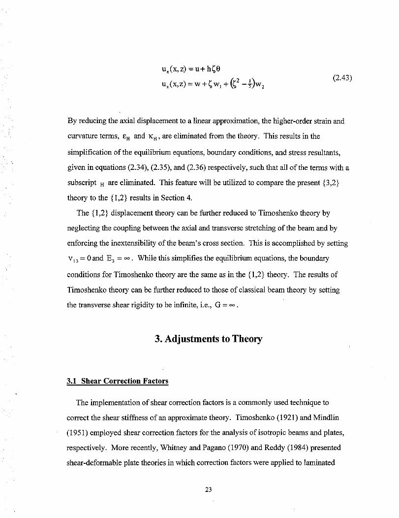
Ux(X, z) = u+ h_O

Uz(X,Z)=w+ (2.43)

By reducing the axial displacement to a linear approximation, the higher-order strain and

curvature terms, eH and rcH, are eliminated from the theory. This results in the

simplification of the equilibrium equations, boundary conditions, and stress resultants,

given in equations (2.34), (2.35), and (2.36) respectively, such that all of the terms with a

subscript rt are eliminated. This feature will be utilized to compare the present {3,2}

theory to the { 1,2} results in Section 4.

The { 1,2} displacement theory can be further reduced to Timoshenko theory by

neglecting the coupling between the axial and transverse stretching of the beam and by

enforcing the inextensibility of the beam's cross section. This is accomplished by setting

v 13= 0 and E 3 = oo. While this simplifies the equilibrium equations, the boundary

conditions for Timoshenko theory are the same as in the {1,2} theory. The results of

Timoshenko theory can be further reduced to those of classical beam theory by setting

the transverse shear rigidity to be infinite, i.e., G = oo.

3. Adjustments to Theory

3.1 Shear Correction Factors

The implementation of shear correction factors is a commonly used technique to

correct the shear stiffness of an approximate theory. Timoshenko (1921) and Mindlin

(1951) employed shear correction factors for the analysis of isotropic beams and plates,

respectively. More recently, Whitney and Pagano (1970) and Reddy (1984) presented

shear-deformable plate theories in which correction factors were applied to laminated

23

plate analysis. The aforementioned theories are based on kinematic approximations

which tend to underestimate shear deformation, which results in an underestimation of the

transverse displacement. The shear correction factors compensate, in a gross sense, for

these deficiencies and bring the transverse displacement results closer to those expected

from exact elasticity theory.

The shear correction factor concept is introduced in the present {3,2}-order theory to

improve the response of laminated composite and sandwich beams. For the case of a

homogenous beam, a shear correction factor is not needed due to the higher-order

displacement approximations. The resulting parabolic shear stress field matches closely

that obtained from elasticity theory. For laminated beams of arbitrary material layup, the

shear distribution is only piece-wise smooth through the thickness. This implies that

adjustment of the shear stiffness may be necessary and can be achieved with an

appropriate value of a shear correction factor.

To determine the shear correction factor within the present theory, a straightforward

energy matching method is employed. The approach is to match the transverse shear

energy of the present theory with that of elasticity theory for a particular "benchmark"

problem. Since it is reasonable to expect that in the thin limit, an approximate theory

should produce correct shear stiffness, the matching is performed for very thin beams

(L/2h = 1000). The cylindrical bending problem, for which an exact elasticity solution is

available, serves as our "benchmark" problem (see Section 4). Vlachoutsis (1992) and

others have shown that, for all practical purposes, these correction factors are

independent of the loading and boundary conditions. The correction is therefore

considered a function of the material system used in the analysis. This implies that once

the correction factor is determined for a particular material system, it may be applied to

any other analysis using that same system. Hence, it is sufficient to determine the shear

correction factors from the cylindrical bending problem and the factors may be applied to

other problems without loss of generality.

24

Factoringtheshearcorrectionfactorfrom the {3,2} theoryshearenergyexpression

andequatingit to theexactshearenergyyields:

U exact = _ lTune°rrected (3.1)shear k 2 "-" shear

where -,rTshear_°°r_ect_is the uncorrected shear strain energy of the present theory. Both

UUncorrected and ITexactso "--shearare computed numerically. The parameter k is computed directly by

computing the ratio of the shear strain energies. Note that the transverse correction

factors kz0 and kzl are also set to unity when calculating the shear correction factor as

these factors are still unknown parameters.

It is noted that for laminated beams, the corresponding shear correction factors are

dependent on the material properties and layup of the plies. For each material system, a

new shear correction factor must be computed. In Section 4.4, shear correction factors are

computed for several material systems and layups.

3.2 Transverse Correction Factors

Similar to the manner by which shear correction factors improve the gross transverse

displacement response, the transverse correction factors are used to improve the

thickness stretch response. Mindlin and Medick (1958) showed that with each thickness

stretch mode, i.e. constant and linear, corresponding correction factors can be specified to

improve the transverse normal response of plates. Tessler (1995) used transverse

correction factors for problems pertaining to the vibration of elastic plates. These factors

were used to rectify the neglect of inertial effects in the transverse normal equations.

While previous theories utilized correction factors to improve the dynamic response of

plates, the present theory will extend the application of transverse normal correction

factors to the static analysis of laminated beams. It was noted earlier that the {3,2}-order

25

theorywithout theuseof transversecorrectionfactorscanyield

following transversenormalstressboundaryconditions

_,. (x,+h)= q+, fL.,(x,-h) = q-

up to 50% error for the

(3.2)

These transverse normal stress boundary conditions are not explicitly enforced in the

present theory. Because of this, the transverse stress distributions may deviate from the

exact solution. For sandwiches with large variations in the elastic moduli through the

thickness, these errors become even more pronounced. This error is illustrated in Figure

3.1 for a sandwich beam in cylindrical bending in which the core properties are more than

three orders of magnitude softer than the face sheets. The uncorrected curve (i.e., without

the use of transverse corrections) shows the large error in the transverse normal stress on

the top surface.

Similar to the shear correction factors, the transverse correction factors are dependent

on the material system, so a set of values for kz0 and kzl must be found for each layup.

To calculate the transverse correction factors, it is convenient to introduce an alternate

form for the beam constitutive relations, equation (2.36), relating the force and moment

resultants to the corresponding strain measures and curvatures, i.e.

where

[E0] =

-All A12 A13 Bll B12 BI3-

A12 A22 A23 B21 B2z B23

A13 A23 A33 B31 B32 B33

Bll B21 B31 D11 D12 D13

B12 B22 B32 D12 D22 D23

B13 B23 B33 D13 D23 D33

, [kz]=

-1 0 0 0 0 O

0 kzo 0 0 0 0

0 0 1 0 0 0

0 0 0 1 0 0

0 0 0 0 k_l 0

0 0 0 0 0 1

(3.3)

26

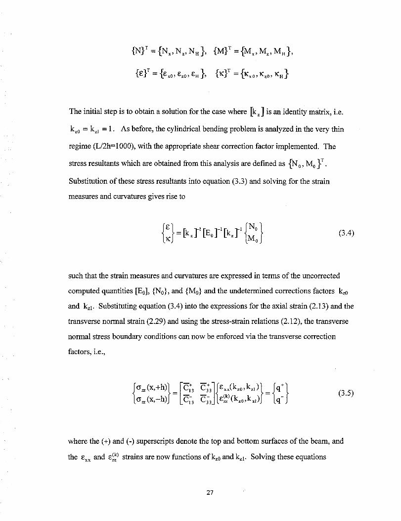
{N}T= {Nx,Nz,NR},

{eY: {_xo,_o,_ },

The initial step is to obtain a solution for the ease where [k z ] is an identity matrix, i.e.

kz0 = kzl = 1. As before, the cylindrical bending problem is analyzed in the very thin

regime (L/2h=1000), with the appropriate shear correction factor implemented. The

stress resultants which are obtained from this analysis are defined as {No, M 0 }T.

Substitution of these stress resultants into equation (3.3) and solving for the strain

measures and curvatures gives rise to

0 (3.4)

such that the strain measures and curvatures are expressed in terms of the uncorrected

computed quantities [E0], {No}, and {M0} and the undetermined corrections factors kz0

and kzl. Substituting equation (3.4) into the expressions for the axial strain (2.13) and the

transverse normal strain (2.29) and using the stress-strain relations (2.12), the transverse

normal stress boundary conditions can now be enforced via the transverse correction

factors, i.e.,

Fc--;,o=(x,-h)J=L_; e';d[e_'(kz0,k,,)J={_:} (3.5)

where the (+) and (-) superscripts denote the top and bottom surfaces of the beam, and

the exx and e_) strains are now functions ofkz0 and kzl. Solving these equations

27

simultaneously for kz0 and kzl results in the numerical values for the correction factors

that fulfill correct traction boundary conditions. By satisfying equation (3.5), the

distribution of the transverse normal stress through the thickness closely follows that of

elasticity theory, with correct traction conditions enforced on the surfaces. Figure 3.1

illustrates this improvement for a sandwich beam in cylindrical bending subject to the

normal tractions: q÷ = 1.0, q" = 0.0 (refer to Section 4, Case D, L/2h = 100 for a detailed

description of the problem).

This procedure is followed such that a set of correction factors is produced for each

material system investigated. A table of transverse correction factors for the material

systems examined in this report can be found in Section 4.4.

0.5

0

-0.5

-1-0.4

iI " "" I" " "tl " " "1 "" " _'" "

_Exact ! i _- ! ,"..... Corrected ! i/;,'i i /i

----Uncorrected| _tj i.'!.......i........i........T........i.........i_:i.......i:_.........i.......

...............i' '.........!.........!.......................,.................,.........,...........,.........,. ,........................." "'' " ..i .i..,i..,iii'"I i i i,,,i ii./i.-i i i i i i i...i_.._i" i...i...

0 0.4 0.8 1.2 1.6

_zz

Figure 3.1 Transverse Correction for a Sandwich Beam

3.3 Integrated Interlaminar Shear Stress

The present theory approximates the transverse shear strain qtxz, equation (2.15), as a

continuous parabolic function through the thickness. This allows accurate modeling of

shear strain and stress through the thickness for homogeneous beams. While the parabolic

strain satisfies the traction-free boundary conditions, the actual shear strain distribution in

8 :

laminated beams is often discontinuous at the ply interfaces. The parabolic

approximation for the shear strain yields erroneous shear stress, as demonstrated in

Figure 3.2 for an unsymmetric cross-ply graphite/epoxy laminate (refer to Section 4, Case

C, L/2h = 100 ). Here, the shear stress for the present higher-order theory (HOT) is

obtained directly from Hooke's law using equation (2.12), resulting in a discontinuous

shear stress distribution. For the exact solution, the opposite is true, i.e., the shear stress

is continuous at the ply interfaces while the shear strain is discontinuous.

0.5

1 1"_- " " ! .... I .... ! .... ! .... I .... I ....",,,,," .: ; :. , ,

k ._. .: .-" _ i--Exact |

\ i "'-_ i i I..... "°TI

.....t i""Ji.............. i..........._i'-

..........i..........i..........._.......:,....[ _L/......

: - . , • : :{ : : • : : :

" i _" i i i.-" .: _. : - :.-" : • : : : :..............: : .- o,." : :

.- - ..,,,, ! - • :

: "":" " " ",, ,i

0 10 20 30 40 50 60 70

0

-0.5

-1

0.5

[j 0

-0.5

--'-,,_ I " " " ! " " " I " "" I " " "! " " - ! " " +

".--•. i i i " "\ .-" --i • ; I--E_a_tl\ " -"",. " " I..... HOTI\i i "._- i ' .- :'

i i"',:'. ° °i i i i _•: .: • _ •i ! ": i ',

_ i .'_.- :- • j, •

. . , .!," .:.......... . ........... -......... ._,_...,L .x........... !.....................

i i __" i i i

4 10"s 8 10"s 0.00012

I_XZ "YXZ

Figure 3.2 Comparison of Shear Stress and Strain for an Unsymmetric Laminate

To improve the transverse shear stress and strain predictions, the two-dimensional

equilibrium equation of elasticity theory

(k) + (k) = 0(_xx,x "lTxz, z (3.6)

is integrated to recover the transverse shear stress. The axial normal stress is

differentiated, then integrated piece-wise through the thickness, such that the resulting

shear stress takes the form

29

1:(_) = _ fz cr(k ) dz (3.7),Lh-- xx, x

The shear strain is then obtained directly from Hooke's law:

_/(k) __ (k) /'_(k)xz qTxz "5 5 (3.8)

The above integration scheme is a well-established approach which generally produces

adequate results (refer to Whitney (1972) and Reddy (1984)). However, for

unsymmetric and sandwich laminates, the integration approach by itself yields rather

inaccurate shear stresses. For such laminates, the integrated shear stresses do not satisfy

the top boundary condition even though the shear stress on the bottom surface is

explicitly set to zero for integration. The comparison of the integrated shear stress to that

of the exact solution leads to the conclusion that error is accumulated as a result of the

shear stress integration through the 0 ° plies. The axial stretching of the midplane, a

characteristic of unsymmetric laminates and soft-core sandwiches, introduces an error in

these plies. The "integrated" curve in Figure 3.3 represents the integrated shear stress

according to equation (3.7). The results are for the same material system as in Figure 3.2.

1- ! - _ . ! : - . ! -

i i _ I Exact

Ik Error Function [ _ _..... Integrated

"_" _ " _'1 " !-- - - Corrected0.5 " ! i ; ;

i i ! _',. i: ; I :

! n:................. •_....B ............ _............ ..%..._.................. 1 ................

i i t:: ,Eo5 ..................i., .............i i ;:--"! .................

0 20 40 60 80 100

_xz

Figure 3.3 Integration Errors Caused by Stretching of the Midplane

3O

For the unsymmetric and sandwich laminates examined, the integration errors are

distributed linearly through the 0 ° plies, while in the 90 ° plies and the core material the

error is constant. To correct for these errors, an automated procedure is developed in

which the total error at the top of the beam is divided into equal increments based on the

number of 0 ° plies. The error is subtracted from the integrated stress curve as linear

functions through the 0 ° plies, and as a constant function through the 90 ° plies, as

depicted in the "Error Function" curve in Figure 3.3. Using this modified integration

scheme, the corrected shear stresses are computed as

con- (k) error (3.9)"l;xz = "_xz -- %xz

where _(k) is the integrated shear stress obtained using equation (3.7) and the error"Lxz

function is expressed analytically as

N

qyxe_°r = _ Fk(Z ) _k(Z) (3.10)

k=l

where N is the total number of plies in the laminate and F k is expressed in terms of

Heaviside functions as

Fk(Z ) = H(z - hk__,") - H(z - h k ) (3.11)

The shear stress error function within the ply is defined as

'_+or ( Z--hk-1"_k (Z) = _k-I + (Z ....

M _hk-- hk_ 1 (3.12)

where "Ok_1 is the value of the error function at the bottom ply interface, and is initially set

to zero ( % = 0 ) at the bottom surface of the laminate. %+or is the magnitude of the error

31

at the top surface of the beam, M is equal to the number of 0 ° plies in the laminate,

and _ is a tracer which takes the form

1, [3=0 °o_= 0, [3=90 ° or core(3.13)

where [3 is the rotation angle of the ply, as per Figure 2.2. The thickness of the ply is

defined as t k = h k - hk_ x, where h k is the distance from the midplane to the top surface

of the ply and hk_ 1 is the distance from the midplane to the bottom surface of the ply.

The variables used in equation (3.12) are depicted in Figure 3.4 for an unsymmetric

composite beam with the lamination sequence [0/90/0/90]T.

Z

[3= 913

[_ =0 °

13=9ff

I_=0 °

6"'-- %,o_ zNII

dP_-l

J/

d

II

/Jf

%

h N

hN- i

h I

]N=4'M=_ ho

th

h

x

Figure 3.4 Error Function and Lamination Notation

As a result of this correction, the traction free boundary conditions are satisfied on the

top and bottom surfaces, and the through the thickness distributions are in close

agreement with the elasticity solution, as evident by the "corrected" curve in Figure 3.3.

32

Although not shown, the corrected shear strain is computed using equation (3.8), and

excellent correlation to the exact solution is achieved. The shear stress distributions for

the cases investigated in this report are in close agreement with corresponding elasticity

solutions (refer to Section 4.5 for additional examples). Note that due to limitations in the

exact solution, Burton and Noor (1994), only cross-ply laminates were considered for the

cases investigated in this report. The present theory is capable of handling arbitrary

angle-ply orientations, but the effect of these orientations on the integration scheme has

not been investigated.

With the exception of the homogeneous case, equation (3.9) will be used for the

recovery of the transverse shear stress for the results presented in Section 4. It should be

noted that the modified stresses may not exactly satisfy the original beam equilibrium

equations. Since the modified shear stresses yield significant improvements for thick

laminates and sandwich beams, this constraint is relaxed in order to achieve a more

meaningful recovery of the transverse shear quantities.

33

4. Cylindrical Bending Problem

4.1 Closed-Form Solution

To assess the capability of the {3,2}-order theory, a closed-form solution to the

cylindrical bending problem is formulated and compared to the corresponding exact

elasticity Solution. Cylindrical bending is a special case of plate bending in which a sine

load is applied to the top surface of the plate, as shown in Figure 4.1. The depth of the

plate is infinite in the y-direction and the ends of the plate at y = 0 and y = oo are

constrained by smooth, rigid planes such that a state of plane strain is achieved in the x-z

plane. The plate is simply supported at the ends x = 0 and x = L such that the resulting

deformation is uniformly cylindrical in shape. Because each cross section in the x-z plane

deforms identically, a beam theory in a state of plane strain may be used to determine

solutions which are identical to those obtained from plate theory.

x

Figure 4.1 Cylindrical Bending Problem

Pagano (1969) first published elasticity solutions for unidirectional (0 °) and bi-

directional (00-90 °) composite laminates in cylindrical bending. Burton and Noor (1994)

developed three-dimensional elasticity solutions for laminated and sandwich rectangular

plates. As a special case, the Burton-Noor formulation yields an exact solution for the

cylindrical bending problem. The exact Burton-Noor solutions are used for comparison in

the present study.

34

For thecylindricalbendingproblem,the loadingson thetopandbottomsurfacesof theplatearedefinedas

q+(x) = qosin(nx / L )

q-(x)=O(4.1)

where qo is the amplitude of the loading. For the solutions presented here, a unit

amplitude will be considered. To solve the equilibrium equations derived for the present

theory, equations (2.39) - (2.43), the kinematic displacement variables are assumed to

have the form

u = U cos(rex/L),

w=W sin(gx/L),

0=o cos(nx/L)

w, = W1sin(gx/L), w 2 =W 2 sin(gx/L)(4.2)

The nature of these assumptions is such that the boundary conditions at the ends of the

beam, equation (2.36), are all satisfied and take the form

@x=0: @x=L:

_x0= Nx(0)

Mx0 = Mx(O)

MIo = NH(0)

M2o = M S (0)

5w(O) =o

8w 1(0)= 0

8 w2(O)= 0

N'xL= Nx(L)

M'×L = M x (L)

M-'IL= N H(L)

'M'2L_- Mu(L )

5w(L)= 0

8w,(L) = 0

6w2(L)=O

(4.3)

Using the displacement assumptions in (4.2), the equilibrium equations are simplified

such that the trigonometric functions factor out in each equation, leaving only the

35

amplitudesU, O, W, W1,andW2,asunknowns. Once the displacement amplitudes are

determined, the kinematic variables are completely defined, giving rise to the strain

measures and curvatures. The strains, stresses, and displacements are then calculated and

plotted through the thickness for comparison to the elasticity solution.

4.2 Material Properties

An extended range of commonly used aerospace material systems will be investigated.

These include a homogeneous case, such as aluminum, fiber reinforced graphite / epoxy

composites for symmetric and unsymmetric bi-directional laminates, and sandwich beams

composed of stiff graphite/epoxy face sheets with soft core materials. Two core materials

are used for the sandwich cases: isotropic polyvinyl chloride foam, the most commonly

used core material (Zenkert,1995), and titanium honeycomb, which can be modeled as an

equivalent orthotropic material. Titanium honeycomb sandwiches are currently being

considered by NASA for use on the High Speed Civil Transport (HSCT). The material

properties are summarized in Table 4.1.

36 •

Aluminum (AI):

Graphite / Epox_(Gr/Ep)

Polyvinyl Chlorid_(PVC):

Titanium Honeycomb(Ti)

E= 10.8 Msi, v = 0.33, G =4.06 Msi

E, = 22.9 Msi, v Lv = 0.32,

E-r= 1.39 Msi V-rv = 0.49,

G,T = 0.86 Msi,

G_ = 0.468 Msi

E = 15.08 ksi, V = 0.3, G = 5.80 ksi

E 1 = 62.36 psi, V13 = 5.6x10 "5, G13 = 75.1x103psi,

E2 = 41.27 psi, V23 = 3.7x10 "5, G23 = 56.7x103

psi,

E3 = 345x103 V_2 = 1.23, G_2 = 1140 psi;psi,

L = Longitudinal Direction (fiber), T = Transverse

1,2, & 3 = principle material directions

Table 4.1 Material Properties

4.3 Test Case Definition

Six test cases are investigated using the material systems given in Table 4.2. While

isotropic materials have identical material properties regardless of the orientation in the

coordinate frame, orthotropic materials, like graphite/epoxy, are commonly oriented in

various directions in the x-y plane to achieve the desired stiffness characteristics. The

layup colunm in Table 4.2 gives the order of lamination, beginning with the bottom ply at

z - -h, and the angular orientation of the longitudinal fiber direction for the Gr/Ep plies

with respect to the x axis. The S subscript denotes symmetry with respect to the

midplane of the beam. For unsymmetric laminates, the total layup must be given and is

denoted by the T subscript. The unsymmetric cases will test the coupling effect between

the stretching and bending modes of the beam. Because of the theoretical restrictions on

37

the exact elasticity cylindrical bending solution, only bi-directional 0 ° and 90 ° orientations

are used in the analysis.

Case Material Layup

A"

B:

C:

D:

E:

F:

A1

Gr/Ep

Gr/Ep

Gr/Ep - PVC

Gr/Ep - Ti

Gr/Ep - PVC

Homogeneous

[ 02/902/02/902 ]s

[ 04/904104/904 IT

[ 04/902/04/902/04/ PVC Core ]s

[ 04/902/04/902/04/ Ti Core ]s

[04/902/04/902/04/ PVC Core/904/02/904/02/904 ]r

Table 4.2 Definition of Test Cases and Corresponding Ply Layup

The ply thickness, tk, for each graphite/epoxy lamina is set equal to 0.00625 in. This

is a reasonable assumption for the actual thickness used in the manufacturing of

composite laminates. The total thickness of the beam for the isotropic Case A and the

sandwich Cases D, E, and F is 1.0 inch. The cores for the sandwich cases comprise 80%

of the total thickness of the beam. For the composite laminate, Cases B and C, the total

thickness is equal to 0.1 inch. The length of the beam will be varied to achieve the desired

span to thickness ratio.

4.4 Correction Factors

The analytic solutions of the {3,2} theory rely on the use of appropriate shear and

transverse correction factors. Following the procedure in Section 3, the correction factors

are calculated for very thin beams (span to thickness ratio L/2h = 1000) and are

summarized in Table 4.3.

38

Case k 2 kzo kzl

A 1 .C 1 .C 1.0

B 0.9105E 1.C 0.96494

C 0.76187 1.21668 1.01975

D 0.30666 1.24326 1.59569

E 0.85883 1.14298 1.26431

F

Table 4.3

0.33811 1.24914 1.59787

{3,2} Theory Correction Factors

Note that the unsymmetric Cases, C and F, require a significant amount of shear

correction as compared to the symmetric cases. This is because non-symmetry causes a

coupling effect between the stretching and bending modes of the beam, resulting in a

significant stretching of the midplane.

To afford a numerical comparison to the { 1,2}-order theory, the corresponding

correction factors for that theory are also computed and summarized in Table 4.4.

Case k 2 kzo kzl

A 1.0 1.0 1.0

B 0.9779_ 1.0 1.0

C 0.7326_ 1.0 1.0

D

E

F

Table 4.4

0.37301 1.24326 1.76405

1.04737 1.14298 1.39621

0.4121_ 1.24326 1.76405

{1,2} Theory Correction Factors

4.5 Results

Six test cases are investigated over a full range of span to thickness ratios. For each

case defined in Table 4.2, thin, moderately thick, and very thick beams with the span to

thickness ratios L/2h = { 100, 10, 4 } are analyzed. A unit beam width is assumed. The

displacement, stress, and strain distributions through the thickness of the beam are

39

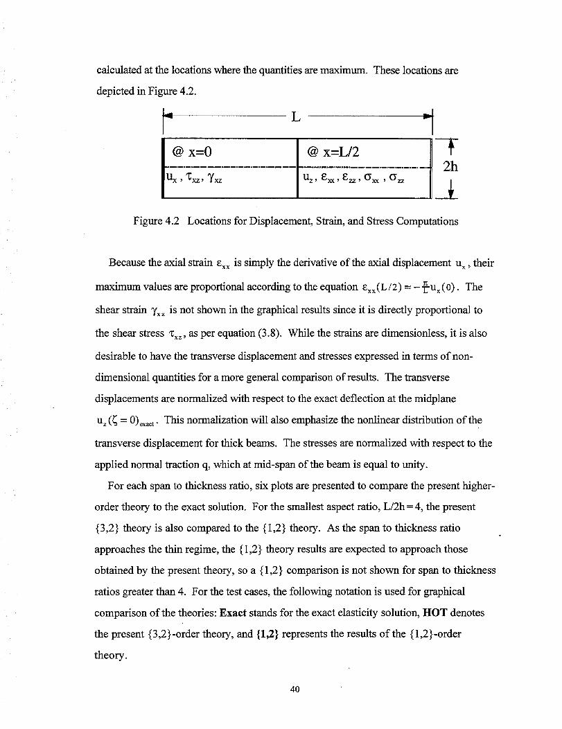
calculated at the locations where the quantities are maximum.

depicted in Figure 4.2.

-I L

@ x=0 @ x=L/2

These locations are

w

• °m°m°m°mm ................. m,m_ n.mOMIm°_._°N° ........ _°m°m .....

Ux, _xz, 7xz Uz, Exx, Ezz, O'xx , O'zz

Figure 4.2 Locations for Displacement, Strain, and Stress Computations

Because the axial strain exx is simply the derivative of the axial displacement Ux, their

maximum values are proportional according to the equation exx(L/2) = -_-u x (0). The

shear strain Yxz is not shown in the graphical results since it is directly proportional to

the shear stress "Cxz, as per equation (3.8). While the strains are dimensionless, it is also

desirable to have the transverse displacement and stresses expressed in terms of non-

dimensional quantities for a more general comparison of results. The transverse

displacements are normalized with respect to the exact deflection at the midplane

u z(_ = 0)exact. This normalization will also emphasize the nonlinear distribution of the

transverse displacement for thick beams. The stresses are normalized with respect to the

applied normal traction q, which at mid-span of the beam is equal to unity.

For each span to thickness ratio, six plots are presented to compare the present higher-

order theory to the exact solution. For the smallest aspect ratio, L/2h = 4, the present

{3,2} theory is also compared to the {1,2.} theory. As the span to thickness ratio

approaches the thin regime, the {1,2} theory results are expected to approach those

obtained by the present theory, so a {1,2} comparison is not shown for span to thickness

ratios greater than 4. For the test cases, the following notation is used for graphical

comparison of the theories: Exact stands for the exact elasticity solution, HOT denotes

the present {3,2}-order theory, and {1,2} represents the results of the { 1,2}-order

theory.

40

4.5.1 Homogeneous Beams

Case A assesses the accuracy of the theory for analysis of homogeneous materials.

As demonstrated in Figures 4.3 - 4.5, the displacements, strains, and stresses, for both the

{3,2} and { 1,2} theories, produce excellent correlation with exact elasticity solutions.

This is accomplished without the use of shear or transverse correction factors. Notice

that as the span to thickness ratio decreases, the transverse deflection takes on a parabolic

distribution through the thickness. For very thick beams (L/2h = 4), this deflection varies

up to 3% of the nominal midplane deflection. The axial displacement, strain, and stress,

as well as the transverse strain all take on linear distributions through the thickness

regardless of the span to thickness ratio. At this point, the present {3,2} displacement

theory does not provide any benefit over the { 1,2 } theory, but the results shown here are

presented to demonstrate the accuracy of these theories for commonly used homogeneous

materials.

The results in Figures 4.3 - 4.5 are expected since the exact normal strain and shear

strain distributions are closely approximated by linear and parabolic distributions,

respectively. These distributions are easily captured with only a linear axial displacement

assumption and a quadratic transverse displacement. Note that both {3,2} and { 1,2}

theories have a unique advantage over previous higher-order shear deformation theories:

they satisfy the traction-free boundary conditions without the need to integrate the

equilibrium equations of elasticity. Many of the higher-order deformation theories do not

satisfy the traction-free boundary conditions and cannot produce accurate shear stress

results without integrating the equilibrium equations of elasticity theory. Though not

shown, results of similar accuracy can be obtained for homogeneous orthotropic beams

without the use of correction factors, i.e., k 2 = kz0 = kzl = 1.0.

41

_;t,

00[ = qz/'-I 'tunu.rtunlv :V osg;:D E'_ oang!_I

b/zxz

09 Ot_ 0£ O_ 0 t

................ j • , ,

............. ":................ !"............... I ................ I...............

.... i.__,i .... i ....

l.-

_'0"

o

S'O

b / ZZ.o

8'0 9"0 t,'O g'O

...... I , , . I ' • • I • • '

iiiiiiii!iiiiiiiiiiiiiiiiiiiiiiiiiiiiiii!iiiiiiiiii, , ....... I I I r I I I t

9"0-

9'0

b/xx£)

0cOl. 8" cOt t_ cOL tw

• ., i,. ,i,,. i ,., i..,i .,, i .......

.........i..........!.........i.........i.........i.......i.................:)l. g-

t-

9'0-

o

9"0

=3

EO00"O tO00'O 0 LO00"O" _000"0-

' _1 .... I .... I .... I .... I ' '

......_..............._...............•..............._................_.......J

,,i .... i,,_i .... i .... _

9"0"

o

9'0

I.

XX_ _ X 1I_-

9000"0 8000"0 0 £000"0"

' ' I .... I ' ' I ' ' t ' ' I ' ' i '

........ •_'......... _.......... _.......... ' ......... _......... 4.......... _.........

9000"0-t-

9"0"

o

9"0

'_(o)_n / _n

_O't tO't

.... i .... i''''l ....

........ ":.......... t .......... _,................... } ......... ,.t'-......... _ .........

........t.........i..........i..............................°...................1 t t

I, . .I

* . * * I .... I' ,,* I**l, * t l l I t , , * I l l , i I ....

66"0 86"0

.... 1 .... I .... i .... l."

9"0"

o

9"0

0.5

0

-0.5

-10.98

.... I .... U ........ I .... I .... I''''l''''

•" : = : • .

! i m ExactI: i :i i ..... HOT I

........ i .......... ':-......... _....... _.......... _.......... _......... ..'.........

....i....i........i........i....0.99 1 1.01 1.02

U z / UZ(0)Exac t

0.5

0

-0.5

-1-6 10 "8

' ' l • • .I , , I • ' :I • , l , , :l • , #O p ,

.........i...........i.........._.........'........._.........._...........i.........

-3 10 "_ 0 3 10 "s 6 10+

-_U x , Exx

0.5

-0.5

-1

............i.............i..............i.............._ .............L............

....i....i ,,,-2 10"_ 0 2 10"s

_ZZ

0.5

0

-0.5

I ...!...!...!..._....... j ......

. . . i i i

-1-80 -60 -40 -20 0 20 40 60 80

Oxx / q

0.5

-0.5

-1

......... , , , . , ,

0 0.2 0.4 0.6 0.8

Ozz / q

0.5

0

-0.5

-1

0

..............i"i.............i...........................................

1 2 3 4 5

Zxz / q

Figure 4.4 Case A: Aluminum, L/2h = 10

43

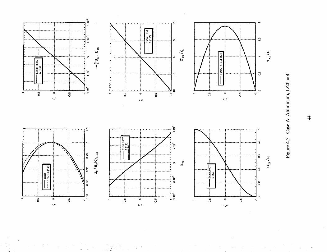
'90

° ° ° " i ...... ' " ' ' ° '

U_

%

.... i .... i .... i .... 'o

o o

O0

T<

I

..... | .... | ........ _..

..................i7 °................]..................

o o,

.... I .... ! .... i ....

• ! ! i

...

.... , , , , .... i , . i

d ?

b

.. o

o

%

d _o

0

u2.o

o

tO 0 _0.

cod

o

o

II

OO

4.5.2 Laminated Composite Beams

Figures 4.6 - 4.8 depict through the thickness distributions of displacements, strains,

and stresses for very thin (L/2h = 100), moderately thick (L/2h = 10), and very thick (L/2h

--4) symmetrically laminated composite beams. The material system is that identified in

Table 4.2 as Case B. Similar distributions for an unsymmetric laminate, Case C in Table

4.2, are shown in Figures 4.9 - 4.11.

Figure 4.6 depicts displacement, strain, and stress results for a symmetrically

laminated, thin beam. The {3,2} results are in excellent agreement with the exact

solutions. While the transverse normal stress varies slightly from the exact curve through

the thickness, the midplane stress and surface tractions are all accurately recovered. In

Figure 4.7, the thickness distributions for the moderately thick case remain in close

agreement with the elasticity solution. Figure 4.8 compares the results of the { 1,2},

{3,2}, and exact solutions in the very thick regime. At the midplane, the transverse

displacement is within 1% of the exact solution for both approximations, whereas at the

top surface the difference is about 6%. The {3,2} cubic approximation of the axial strain,

exx, produces accurate maximum values at the top and bottom surfaces, whereas the

{ 1,2} linear distribution underestimates these maximum values. This results a 20%

underestimation for axx when the { 1,2}-order theory is used. This discrepancy is

especially significant when designing a laminate according to the maximum stress criterion.

For the case of an unsymmetric laminate, the midplane exhibits straining due to the

axial and transverse strains and the coupling between the two stretching modes. In Figure

4.9, a tensile ex× and a compressive e,z are observed at the midplane. In Figures 4.9 and

4.10, close agreement is shown for the through the thickness distributions, with the

exception of the transverse normal stress _zz- The midplane stretching results in a _=

thickness variation that is not captured by the higher-order theory. In Figure 4.11, the

{3,2} theory shows improvements over the {1,2} theory for very thick beams, although

the polynomial distributions are unable to capture the piece-wise smooth, exact solution.

45

1 .... I .... I .... I ....

o.s ..............................!..........

i._ 0

-0.5

-1 .... I .... I .... I ....

0.98 0.90

-- Exact & HOT Ii

+......... I .......... :-......... ,{.........

.... J .... I . ,i I I ill l

1.01 1.02

u z / Uz(0)Ex=t

0.5

0

-0.5

-1-0,0_4

....+....+....+....i....+....+....!" "--Exact&HOT i ! !I I + + +

......... +-......... " ........ +......... .+-......... i......... -+.......... ++.........

-0.0002 0 0.0002 0.0004

---_U ExxL X _

1 .\ ..... i...._......... i....i....+....

o.s........_.. ............ i........._.'+.........J.........

_ 0-0.5 ......... _"......... '_ .......... :"........ _ ,1" ......... { .......... :" ......... { ........., ....i....i....J.....°0.0002 -0.0001 0 0.0001 0.0002

_zz

1

...... I ' ' ' I ' ' ' I ' " '_,. ' ' '

o.s i-- Ex_ _.o"," i i +

o!!!!!!,++iiii+iiiiiiiiiiii-0.5

.+.../i=fl ii...... i..,-1.2 10 + -8 103 -4 103 0 4 103 8 103 1.2 104

Oxx / q

0.5

0

-0,5

........ ' I ' .....

.... i i ,''...............+'--_aml +

.........i++................++................++................++..............., , , i , , , | , , . | . , , i , , ,

0 0.2 0.4 0.6 0.8

0.5

0

-0.5

-1

...... j ............

0 10 20 30 40 50

(Yzz/ q 'rxz / q

Figure 4.6 Case B: Gr/Ep Symmetric Laminate, L/2h = 100

46 +

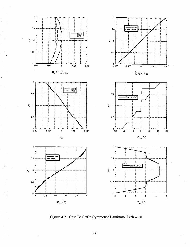
0.5

0

-0.5

-10.98

.... i iI .... ! ' " "!!'._i i i i'"' .............. ' ....

iI

III

I

_ Exact I"'"'"°I I

i|

:Jie

: : J :

i i e i

.... i .... i_'.. ,, .... , .... , .... ! ....

0.99 1 1.01 1.02

u z / Uz(0)Ex_:t

0.5

0

-0.5

-1-4 10 "6

....i....i....i....i....i....i....ii/-iLE_ctI _ i "'/t

iiiililili,i i i i........i.......t......... i.......... " ....... i.......... i.......... _.......... i.......... _.........

-2 10"e 0 2 10 "e 4 10"_

-"CUx, Exx

0.5

-0.5

-1-2 10 "e

............ e. ......... _.......... _......... _........ i ......... _.......... _.........

............i..... 1-1 10 "_ 0 1 10"_ 2 10 "_

_ZZ

0.5

0

-0.5

-1-12_

............ _ ............. _............. i ............ .i............

I Exact & HOT _ i iI I_ i i

iiiiiiiiiiiiiiiiiiiiiiiiiiiiiiiiiiiiiiiiiii.i i !

-80 -40 0 40 80 120

_xx/q

0.5

0

-0.5

........ ' I ' ' ' t ' ' '

i i .

.............._= HorE_II........../[..........................

./! i i i_i ... i. ,,

0 0.2 0.4 0.6 0.8

0.5

0

-0.5

' • l .... I .... i ........

-- Exact & HOT i i

.............. 4 ................ _............... _.............. _...............

0 1 2 3 4 5

6zz/q Xxz/q

Figure 4.7 Case B: Gr/Ep Symmetric Laminate, L/2h = 10

47

' "% _ _, 1::_._ _ • •

_.oo._: : • : 4

: : • f :

i i • :, :

os 7/._

............................ T ............. , ..............................

i# •

o ........................¢...

• ##J#

i." /-0.8 .............. /.t......... •....

4R i •

/-I . I . Im . • t I , , . I , , , ' , . ,

0.96 0.98 1 1.02 1.04 1.06

,f. ........_................,.........-- Exact I

..... HOT |

----{1,2} I............... 4................. :-..............

U z / Uz(O)Exac t

1...... !'"! ...... , . .. , ._6t ,,w-_.

: i : : i i --

: i ,,_ Exact i :" 0:

05 ..... HOT |..........!.......

i i :_ i: i i • : : :

_ o: : : # :!,_t' : :

-o.6 .." i , _ ! ! i.........I..........F ;'_.........._.........',,.........._............'........

i • i i i ! i

-1 ' i,,,

-8 10 .7 -4 10 .7 0 4 10 .7 8 10 .7

/t

--CUx ' _xx

1 / .... i .... r_=,_ , .... = ....

i i i _. i

I-...... | ..... HOT I ..........i...........i.../h,......i.._........

o ............7.............i .............i......... i.............i............

: :- : !: a: : : :

-0.5 ............. ..-........... _, ....... _.............. _............. !............i _ : : :i i . _i i i

1 10 .7 2 10.7 3 10 "7 4 10 .7

_-'ZZ

1i i i i i i i....,....,....,....,....,....,,_,,,,

_ o

........i-:i- ........................., ,,,_, ....!....i........i....i....

-20 -10 0 10 20

Ox×/q

1

............ I ' ' i

..... : s "

-- Exact _ • "0.5

- .... HOT & {1,2}• , - i . i "

ii;iiii.._" i i i-0.5 ........ • .- ............... .;................ _................ ;..............

-1 .. , ,... , . • . i ,, , i , ,,0 0.2 0.4 0.6 0.8

0.5

0

-0.5

''i .... ! .... i ....

................... :" .................... "i....... ..t ....... _...................

_--_o_ 1.......-...............!it', •.....1_ ............".,,It..........

" _ i i: '

.................. i .................... _....... ', ....... _...................

0.5 1 1.5 2

_zz / q Zxz / q

Figure 4.8 Case B: Gr/Ep Symmetric Laminate, L/2h = 4

48

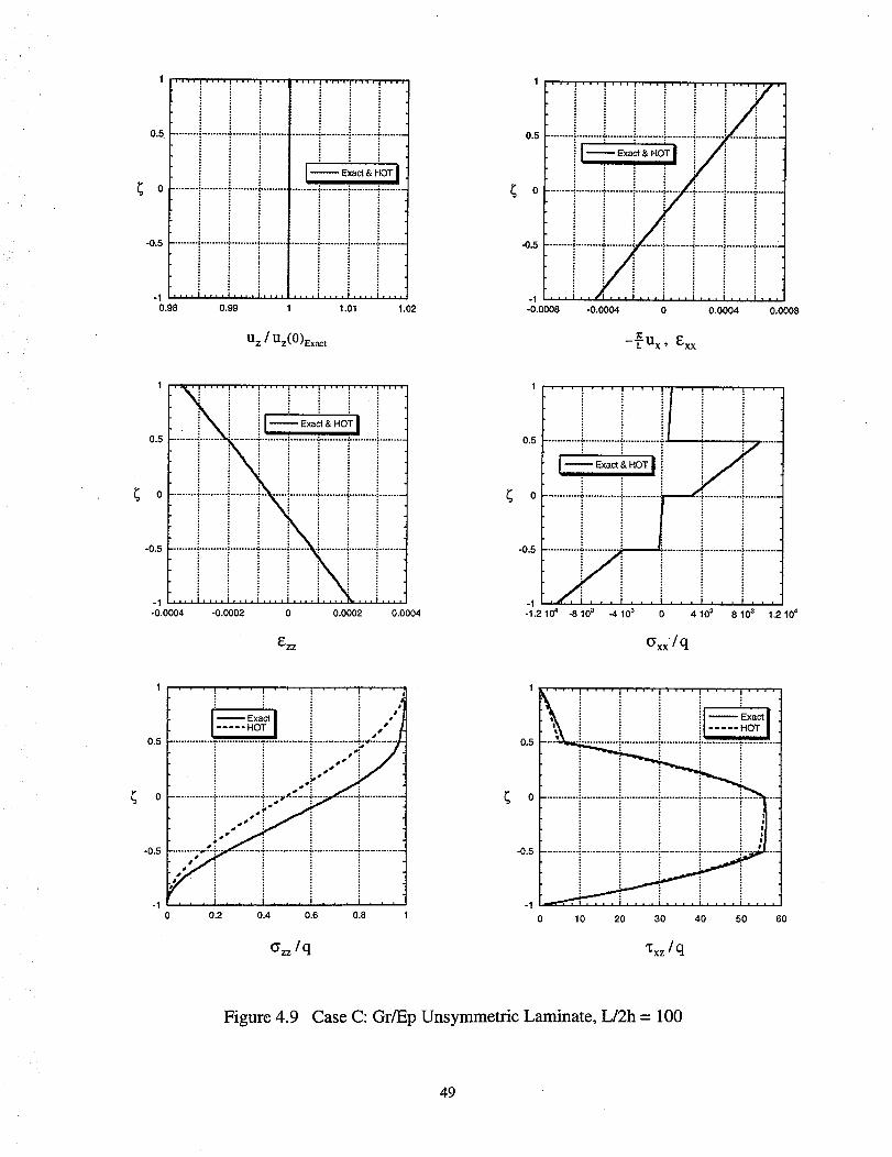
0

-0.5 ......... a......... +......... _.........

._ .... I .... I .... I ....

0.98 0.99

0.5. "............................:.................._.........._........._ ........

l-- =ct,.oTI

......... ¢.......... I..........}........

1.01 1.02

uz / Uz(O)E_a_t

0.5

0

-0,5

-1-0.0008 -0.0004 0 0.0004 0.0008

---_U ExxL x ?

0.5

0

-0.5

I , 'I .... I .... I .... I .... I' ''' I'''' I ....

: i i J i !, ! _ i • i

........_.........._..........4 ......._...........".,........._...........",..........

-I

-0.0004 -0.0002 0 0.0002 0.0004

E'ZZ

-0.5

1..................o._ .........................] ............!] i

I

0 ............ i ............. ' ............. _'

i

-1.2 10 4 -8 10 3 -4 10 a

............].............i............,, ,i . , , i , ,,

4 10 a 8 10 a 1.2 10 4

Oxxl q

I ...... !'''I ......

-- Exact I i "

..... HOT I i : s"l : : •

0.5 ................-..............._ ................-...............-.._..........

: : : ws S :

: : .._s

0 ..............._................$'-'-'=,_-"----'_ .............$...............

: o • . :

-0.5 ": : : :S ° ,

-1 , , , I _ , , I , , , I , , • ' . . •

0 0.2 0.4 0.6 0.8

II_" '' "I_ .... I .... I .... I .... I ....

i i i iI-_ i i i il--Ex,ctl

'1_ i i i :1 ..... HOT I

o.s I-'"_ :"o ............_.............!.............!.............i............._..........

_ _ _ _ ,

-0.5__.............i............._.............i............._............."----'....

0 10 20 30 40 50 60

_z/q "_xz/q

Figure 4.9 Case C: Gr/Ep Unsymmetric Laminate, L/2h = 100

49

0.5

0

-0.5

-10.98

i i • ' " ' '! i :'. : : : :

.... H

......... I ......... o ......... ,¢............... 4 .......... } ......... + ........

.... i .... I .... i ,I .... I .... 1 .... I,,it

0.99 1 1.01 1.02

U z / UZ(0)Ex_c t

0.5

0

-0.5

-1-8 10"e

' " ' I ' ' ' I ' ' " I * • . I ............ • • i • • . i . .Jj,."

i _ i i ,': : : _ .." : _ :

........i.........._.........-..=.........!........._.........i ........i............. HOT : :

........ _.......... i ......... :7 ...... _.......... _......... _.......... _.........

...i ..

-4 10"e 0 4 10"e 8 10"e

---nU ExxL X _

1 .,,_ ,,. ......... . ......b" I''" I I I .... ! '1''..,'.. : _ :

• _R,,,,i": i --Exact|

......_.. w": "o_.io.,.........i..........i......_..........i.........i.........i.........i........i ! :, ! !

_ : • : : : :(_ 0 ........ _.......... _......... _.....a. , ......... " ......... : .......... :........

: : : • : _

i i i ..", i i i_ _ _ _ : : :

-0.5

, ....i i ....-4 10 "e -2 10 "6 0 2 10"5 4 10"_

_ZZ

0.5

0

-0.5

-1

1 " ' ' I ' • • I ' ' ' ! • ' I ' • • I ' ' '

'i ii.............s............._,.............i , _ .....

: _ i

E_ctI iS

I';'"_°_ .......

........................' .............i--------------i--------.....-121 -80 -40 0 40 80 120

Oxx/ q

1 • • • , • , , i , • • i • . , i , .. , _

i i i i ._: : : : •: : : : •

: : : : •

o.s I -- E,,._I i .-_

I-....H°TI i.-"__ _ ." _ ...............

......... .':.."............. -................................ :,...............

-0.5 _ i"•° " i! _ii

-1 , , , I , , , I , , , I , , , I , =

0.2 0.4 0.6 0.8

0.5

0

-0.5

-1

.'"'I .... I ........ I .... I ....

• _ i i i _ Exact_ _ ..... HOT

1 2 3 4 5

Ozz / q 'CxzIq

Figure 4.10 Case C: Gr/Ep Unsymmetric Laminate, L/2h = 10

50

0.5

0

-0.5

-1 ., .i, /0.96 0.98

'' 'I ' ' _' ''_ ......_ ! I_=I i: ,• \ i I ..... HOTI _; /

_........_...:.........._.:.'..:!...!..._./....../...._...............

............... | _, :,

a:

........../_.._/...............................,i/.

//

1,02 1.04 1.06

u z / Uz(O)Exa_t

0.5

0

-0.5

-1

.I.6 10"e

: . _a i........i.l=_:l.....i.............x_,.........

........]..........i........._iiiiiil.i..........t.........

-8 10 .7 0 8 10 .7 1.6 10"6

---_Ux , Exx

1

0.5

_ o

-0.5

-1"4 10 .7 "2 10 .7 0 2 10 .7 4 10 "7

_'--"ZZ

i i........L.ii i i"f°_......_b_li _ '__ .....

-20 -10 0 10 20

Ox_/ q

1 , ..... , , .......

_ Exact I } o °* _7_

............ HOT & {1 2} | ......... :"................ :.--*_-----,.i-qo.s ' : :' ' i :7 /t

: : : _w 'p :

_ L.o •...............i................i-----_,,--'-----i............. .:...............

i o-_ i i

-0.5 "f " ' "

i p :

-1 , . , I , , , I , , , T . , , I , . ,

0.2 0.4 0.6 0.8

0.5

0

-0.5

i ' ' ' I .... I .... I ........

................._- _ ....

0 0,5 1 1.5 2 2.5

_z / q %z/ q

Figure 4.11 Case C: Gr/Ep Unsymmetric Laminate, L/2h = 4

51

4.5.3 Sandwich Beams

Cases D, E, and F address the analysis of symmetric and unsymmetric sandwich

composite beams. Sandwich beams present a unique challenge to the theory owing to the

drastic change in the material properties through the thickness. The face sheets of a

sandwich are stiff in the axial direction to carry the axial stress while the core material

may be considerably less stiff. This is possible because the magnitude of the transverse

shear load is usually much less than the axial load. As a result, the core can be made of a

lightweight, compliant material, reducing the weight of the structure. Typical thickness

dimensions for the components of a sandwich beam are illustrated in Figure 4.12

I Face Sheets

Z

!!!e llllllrlrllllllltlllllllll lllllrlllllllllllllllllllllllllltll

m 0.1

0.4

X

0.4

Figure 4.12 Sandwich Composite Beam

Figure 4.13 shows the results for Case D in the thin regime. Note how the axial stress

(Yxx is carried by the Gr/Ep face sheets on the top and bottom faces of the beam while the

transverse shear stress "Cxzis almost exclusively carried by the PVC core. For the thin

sandwich, the {3,2}-order theory almost exactly matches the exact elasticity solution,

while for the thicker case, shown in Figure 4.14, the limitations in the theory are more

evident. The transverse displacement prediction is about 2% in error. The stresses and

strain on the top and bottom faces, where these quantities are usually the largest, are

accurately predicted by the theory. For the thick regime, Figure 4.15, the transverse

displacement is overestimated by both the {3,2} and { 1,2} theories, with errors ranging

from 12% to 37%. Notice that the linear approximation for the axial displacement in the

{ 1,2} theory underestimates the axial strain, resulting in a significant underestimation of

52

the axial stress. The {3,2}-order theory captures _xx at the top and bottom surfaces

adequately, while the same stress for the { 1,2} theory is 85% in error. The quality of

these results suggests that the span to thickness ratio of L/2h = 4 may constitute a

practical limit of application of this theory for sandwich beams.

In Case E, the sandwich core is made of titanium honeycomb. Because of the

orthotropic stiffness properties of the honeycomb, the axial stiffness is very low

compared to the relatively high transverse stiffness. The sandwich core acts as a shear

web, resisting the transverse stresses only. The titanium honeycomb serves as an efficient

core material, providing a large transverse stiffness with a minimal weight penalty. Figures

4.16 through 4.18 depict the results for the sandwich beam with a titanium honeycomb

core. Note that the nonlinear axial effects are present until the beam approaches the thick

regime (L/2h = 4). Comparing these results to those for the PVC core shows that the axial

displacement and strain are already nonlinear at L/2h = 10. The axial quantities become

increasingly nonlinear as the differences between the transverse stiffness through the

thickness of the laminate increase. This is evident with the larger discrepancy between

the {3,2} and {1,2} results for the sandwich beam with a PVC core. As a result, the

higher-order terms in the {3,2} theory do not provide as much benefit over the { 1,2}

theory for Case E with a titanium honeycomb core.

In Case F, an unsymmetric sandwich beam with a PVC core is analyzed. This

particular sandwich presents the greatest challenge to the beam theory because of the

axial-bending coupling and the low stiffness of the PVC core. Figures 4.19 through 4.21

depict accurate correlations with the exact solution. In Figure 4.21, the benefits of the

higher-order axial displacement over the linear axial displacement are evident. While the

deflection preducted by the {3,2} theory differs from the exact solution by about 8%, the

{1,2} theory prediction is in error by 22%. The axial strain exhibits a highly nonlinear

distribution through the thickness, with the boundary conditions accurately modeled with

the {3,2} theory. Although not particularly evident from Figure 4.21, the axial

compressive stress for the { 1,2} theory is underestimated on the bottom surface by 83%.

53

0.5 ......... :......... --"............................. +.......... =......... _ ........

--Exa= J!I ..... .o'r li

-0.5 ......... _......... -:-......... ':.........

-I .... i .... r.... t....

0.98 0.99

.... i,,,,I,,,,i,,,

1.Ol 1.o2

uz / Uz(O)ex_ct

0.5

0

-0.5

-1-o.ooo4

l '' "I........... I''''I .... i .... I''''I .... I''''

F . i i i i i )

-0.0002 0 0.0002 0.0004

_'-"ZZ

0.5

0

-0.5

-1-o.ooo8

...........,...,...,......._.jt

........-.'.........i..........i.........+..........:......."...................-_

........ _"......... _....... ['......... _.......... _......... _ ......... i.........

. i , ,,

-0.0004 0 0.0004 0.0008

/'C--L-Ux, Exx

1'*'l'''l'''l'''l'''l--''l'''t'''l'''l_'''

0.5 ....... .-....... :........ }....... i.............. :....... ":........ _....... + ......

0 .............................................................................

-0.5 .............................................. : ....................... _ ......

. ! : ! '!

-16000 -8000 8000 16000

(_xx/ q

0.5

0

-0,5

.... , .... ! ' , . [ ' . .

i i ,,

-- Exact II [

.............. _ ..... HOT I ......... t ....... 7_3' ............ ;

: : : =,s :

i i _,-" ii i ,._.° !

i ..'" i i i

, , , I . , , I . . • I . . , I . . l

0 0.2 0.4 0.6 0.8

1 "''_1 ....

) )0.5..................+.........+.........+..........._.........t..................

I__1 )

-0.5 .......................................................... -7 ..................

-1 ._i ....0 10 20 30 40

6zz / q "Cxz/ q

Figure 4.13 Case D: Gr/Ep-PVC Symmetric Sandwich, L/2h = 100

54

0.5

0

-0.5

-10.98

.... | .... |.,, |, .,. |*,,, i||,, ,i, ,,, 1,,, i: : : : : : :

++)+++++: i ! : ,: : :

......... :......... ,.:......... :.......... ?......p..:. ......... :......... .:.........: : : : I: : : : I: : : : #i i : : + : :: : i i a i : ;: : : : • :: ' : : I: : : I : :

......... ; .................. * .......... :..i-.....; .......... ; ......... .p. ........• . . • + . .

I! i i l, i : ': I: : :, : I-- ExactI: / ..... I Ii i i i I i ..... HOT

......... i..----4..':- ......... _.......... +._........ .+.......... +.......... $ ........

i i. i i !, i

i i i il ! i i: ! l P i i: : : :1 : : :: : : :1 : : :

.... I,., I .... I,iI_ll,_+=l,,,tl .... I,.. I

1 1,02 1.04 1,06

u_ / Uz(O)E_ =

0,5

0

-0.5

-1-1.5 10"s

1 ,.. i, o. i . ,, i + ,, i .,. i, ,_|

.........+.........'+':::[...... ._.........+...........,...................j I : : : . :+ P, i -- E_a Ii i ". ! X i i I ..... HOTIi l '%. : :

i i i i _ ",: : ! i _ 0: :

......... _......... <.......... ;......... .:. ........ <........ +=+.......... _.........: : : : : •

i i i i i,-"

-7.5 10+ 0 7.5 10_ 1.5 10 "s

-_U x , Exx

0.5

0

-0.5

1 .... i ' ""_ ' i .... I .... i .... I .... I .... t

• i "%+ + i + i ]i i l l l : +i i i + + i ]

.......... _............ !........... ,:........... ,............. +........... ?.._:....; ; : : : :s

l "''''H°T I + + Z." + _+ + + ;, "i +

l i l ,'" l :l l i .° l i i

: : ,,: i i i

.......... l ........... i----.r'----_ ......... :............ _.......... ÷ ..........

i i: i i i i.... i.... iiiill '-1

-2 10 .s 0 2 10"s 4 10"s

E, zz

i "= • io+ ............................-...........................-...................

I--L-Exactl..... HOT I

0 ......... :-......... ._.......... _.................... + + {

-0._ ............................. i .................... " .............................

., . ...-_. :_, ._..., .... , .... ,...-400 -200 0 200 400

axx I q

I--_I i i J,",

]..... ++! _+o.s ..................-.............. - ............. : ............i i i ,-i

: :a +'¢ :0

: +, : : :

! o" i i i1_ : : :

-0.5 .......... --_- ............. - ............... - ............... - ...............

/a .

-1 . . . I . . . I , . . I , , , 1 . , ,

0 0.2 0,4 0.6 0.8

1

0.5

_ o

.... I + ''':'''TI.t'''l .... I .... I ....

_ _ ___ii i i.....lr.......................... _............... i iI :

g

+ i......liI :

I

-o.s ................................................................. ,_._........I :I :i :

-'t '" i ! .... !.:.: ............. i ....I 2 3

(_+ / q "Cxz/ q

Figure 4.14 Case D: Gr/Ep-PVC Symmetric Sandwich, L/2h = 10

55

.... I .... I I • i_l i i i i , _ .... I , I , . I}l I I

I--Exactl / _ =_ _ _t

I----'HOTI/i "i ! 7I-''_''_1/i !i i i

°_ ........................'/i7 ................'........:_...........li/

: J ; ; f :

o ................................_..:........i...........i.........! _.........i' l i: i

I

I-I i I .... l .... I .... I .I. I I I , i i t

0.8 1 1.2 1.4

u z / Uz(O)E,_ct

0.5

0

-0.5

-1-2 10"s

T\i ...._...._....!.i ....

....r-%!=ii:.......i i/._,Lf........

.........i:...... .........i........i_i i i i

......._i ....i........i.......0 2 10"s 4 10"s 10 "5

0.5

0

-0.5

.... J .... J .... I I • • JI * , I ....

i _ ;, i !i o"'_' Exact

_' I i i: il ..... .o'r............_.........._ ..........fl---_,,_.,

............_.........___._ ............._............

: : | _ : a :: : I: •! i , ! :o" i.... ......

-1 10 "s 0 1 10 "s

-'_U x , Exx

{ 1,2} (3,2

.0.5 ..............................................................................

..... HOT I-- --{_,2} I

I

.o.,..........................................................i.........i........-1 _'''

-160 -80 0 80 160

Ezz Oxx / q

0.5

-0.5

' ' ' 1 ' ' * I ' • * I ' ' ' I ' "_ '

i ! i _..I_ t::xactl i i " " "J..... ,oT[ l--,L_.:.......-

......../--":"_ li...............r"/3:_ ...........

i i ,.9""

_._ .............

......2_?._ ......_ ............• ,': i i i

0 0.2 0.4 0.6 0.8

-0.5 ...........................

_..fP-_-1 -" . i

1

._ i _ * ""_1

0.5 ..................................I................_..........................

I I ..... HOTI

o...................................i..-........J..--...!':L!........Ii

........ o:: .......................................

,i i\_..- .........

2

o= / q Xxz/ q

Figure 4.15 Case D: Gr/Ep-PVC Symmetric Sandwich, L/2h = 4

56

0.5

0

-0.5

-1 .... i .... i .... i ....0.98 0.99

.... i,,, ,i .... i .... i .... i .... i .... i ....

.... I,,,,'l,,,,I,,,,

1.01 1.02

u z / Uz(O)_ t

0.5

0

-0.5

-1-0.0008

........ ,................. i i '

........ •_-......... _.......... :,........ " ......... _......... ._.......... i .........

-0.0004 0 0.0004 0.0008

-'EUx, Exx

' "_"'i ....J....i................

i ! _i I--Ex_O'HOTIo._........-.........i.................. i.........i .........i.........

o............................................!.........!.........i i i i i i '

-1 I I I I I Ir,,,l_=_

-0.0004 -0.0002 0 0.0002 0.0004

0

_"ZZ

1 ''' I'" '1' ''l''' I'' ' I,' ''f ' ''1 ' ' '1'' ",_'''

:. ; ; ;or

0._ ...................... _ .........................................................

0 ..............................................................................

-0.6 ..............................................................................

-1 '''_" ' '1 ' '' I''' I '' '_i ' "i '''i '' ' I'' '1 '' '

- 16000 °8000 0 8000 16000

Oxx / q

0.5

-0.5

Exact" _ i__

...............i"..... "----'

================================......... ,_.." ............. _................ i ................ ::...............

i i • i . , , i , , , i , , , 1 , , ,

0 0.2 0.4 0.6 0.8

0.5

0

-0.5

-1

..................i.........i.........i.........._.........i........

5 10 15 20 25 30 35 40

(_zz / q ':x_ / q

Figure 4.16 Case E: Gr/Ep-Ti Symmetric Sandwich, L/2h = 100

57

1 .... ! .... ! .... ! .... ! ,,IL.._. I .... I .... i ....

i i ! it '

: : : : #: : : : • :: : : : l :

i : : = : : :: : _ : a : : :

0.5 : : : ! ' _ !

I-- Exact I : : : :

.....HOTIi il; i, : : m i |" _ i

: : : l!ii= : i i

0 ........ T ......... :......... ":"........... , ....... : ......... .':"..................: ! i .e _ : :: : : :1 ."

i i i _:: _ _ i' : : :: : : :, _ _

-0.5 ........ -i-......... i .......... _............ _.......... .i...................

: : : f :

i i i ,: i: : : l:

-I .... I .... I .... 1, .,l,,,,l,,,,l ....

0.98 0.99 1 1.01 1.02

u:_/ u:_(O)_ t

0.5

0

-0.5

-1-8 life

• ' ,I.,, I,,,I,,,I, ,|1,,,I.,, I,

: : : : : ,' ! i

: : : ! • : :: : : : • : _ !

! )I.....

. ).iii:i iil.iii.l.i.:..il......... _.......... b-- _...$ ......... i .......... _.......... i .......... ; ........

-4 10"s 0 4 10"e 8 10 "e

--_U x , E:xx

....... I''''I .... I .... I .... l .... I''''

: : : : : I'i i: : : : : /: : : : ; ! : :

I :: : : I : I :

: : : I : I : :

o.5 ........._......... i.......... )......... _......... """ ":'"......... :.........

I__ ,oo 1 ,..... HOT I

0 ............................................................................

:d

l

*0.5 e:......... _ .................... "......... ."T....... "t'.. ...... ? ......... ! .........

1 : : I' : :

-1 .... i .... i .... i .... i .....-4 10"_ -2 10"_ 0 2 10"e 4 10"_

E'ZZ

I .... I .... I .... ! .... )2'''1 .... I .... I_''

• ' ; f i

0.5 ......... _......... v ......... _ .................. ¢.......... _ ......... _.........

I--E_aHOT I

_.5 ......... _ ........................................ =.............................

.1,,_,, .... , .... _ .... , .... _ .... i .... i ....

-2_ -100 0 100 200

_xx/q

0.5

0

-0.5

...... I • ' ' I ' ' ' I ' ' 'd

: : : J[

. . ';... i i _

I..... I i = " "............... ¢ ................ 4- ............... _ ............. ¢--._- ..........

! _ i J"

............... i................

...............................,..............., , , I , • * I • , , I , , * I , , *

0.2 0.4 0,6 0.8

0.5

0

-0.5

" "'_1 ....

........ :........... ;.........:".........)......... T......... i..................

) )

II

i ! i i i i •*_rrll

0 1 2 3 4

Ozz / q q:x_/ q

Figure 4.17 Case E: Gr/Ep-Ti Symmetric Sandwich, L/2h = 10

58

0.5

0

-0.5

-10.9q

0.5

0

-0.5

• .._ . .._..._ ...._,../

..............................................................0.98 1 1.02 1.04 1.06

u z / u_(0)E,_t

1 ..... I ...... I .... I .... I .... I .... I ....

i i i i i_ii i i i i i _i: : : : : . o# :

........_.........".........._........_.........._........._;_I .........ExactI i ! ! i

..... HOT |i _ i_'_

.....!7:;?_!i........_ .........i.........

........-.:".........!---S_-...........................i.........: : a • : : | :

i i,'Zi i i i i

.... i .... i .............. i ....-1-1 10"6 0 1 10 "6 2 10"_ 3 10"8

_ZZ

i '"i''''' ''i

o,........_....................i....._,.,-4,. _i;;_i_'_...............i........i i i ,1..) _ I_,ct I

........ i .......... i ......... ; ...... !._-ff-....... .i ..... " .... HOT ..o _ ' _l'i. _ l--_'_li i i, i" i i :: : ' ! t : :! i /.' i • i i i

-0.5 ......... i.............. i---.--,-._ ........ l.... __-.--_-. ......... i........... ._"........

-1 ' ,a ..... q II , ,, , , , , ,,

-1.8 10 "6 -9 10 .7 0 9 10 -7 1.8 10 "6

-_U ExxL X _

{],21 {3,2}

1 .... i .... i .... i .... !,;,,,, .... , , ,_, , ,_,..,,w_.

..... HOT I

-"{f I_ 0 ........................................ ' .......................................

-0.5 ....................................... | .......................................

"; ; -i

-1 .,,,.,,_ I , .,, . I .... I ,,.,"i .... i .... i .... i ....

-40 -20 0 20 40

O_× / q

1 [ ............ | , , ,

i _.

i o# •

.......... _'_Exact

o,f......._--,--.OT,,,_,,........i_'i'i i _'° i

0

i _- i i: • : : |

i ,,"° _ i ii," _ i i

#. : , ,

-0.5 ...... T;,'--t ............ t ............... _................ ." ..............•" ! i i i

• = i l i• : . . :

0 0.2 0.4 0.6 0.8

" - . ' '-'-,_ ' ..... I ..... I .....

: i

0.5 .............. : ................ .'-............... "."................ :- ...... ....[

I,_a_ct i ;

--"{_'_}liH°T[...............................i"I

I-0.5 .............................................. "........................ _....

i

-1 --, , ,-,_2,,,_, • ..............

0 0.3 0.6 0.9 1.2 1.5

0 ..............

0_ / q "_xz/ q

Figure 4.18 Case E: Gr/Ep-Ti Symmetric Sandwich, L/2h = 4

59

-0.5 ......... =......... ":"......... ¢..........

-1 .... I .... i_..,I ....0.98 0.99

o._........................................................i........._........i -- E=_,Iil ..... .oT I

........ _.......... }......... g,........

.... I,.=t|ttl=w=ll=

1.01 1.02

u z / Uz(O)E=,.t

0.5

0

-0.5

-1-0.002

.... |,o,,i .... i,,,.i .... i .... i .... i ,J_,,

,-- ao,HoTIi/.......................................,.........::......... _.......

........ _.......... i ......... .i........ i ......... 4....L...i .......... i.........

....i....i..... !....-0.001 0 0.001 0.002 .

-£U ExxL X _

1 • '_1 ......... i .........

0 --

-0.5 .................... ------4 ........................... _........................

-1 ......... i tl

-0.001 -0.0005 0 0.0005

_"zz

1I .... I .... I .... I .... !l''''l .... I .... f'''

[ t I I

0.5 ........ i .......... _......... -.'.................. :.......... .:.......... :........

t--E,a_,,,,oTI_ 0 .............................................................................

-0.5 ...................................... •.......................................

-1 .... ; .... i .... , .... t ........

-40000 -20000 0 20000 40000

axx/q

0.5

-0.5

......... 0 , , , , ,

i ##,

i so .

..................1-- E== I.....-..........i I ..... .orl i /._.."

• i _ _"

i .fi i i

_;/¢ ...................

i i i ] i i i ...... I , , •

0 0.2 0.4 0.6 0.8

1 ........ ! .... I "'_,._._.... _.... I .... J....

: i! ,

0.5 ................................................. :'........._------a..........

'--'Exact i

I..... .or I

-0"°......................................i....................i..............._ ,:

i i :-1 '_ ....

O 10 20 30 40

(_zz / q _;= / q

Figure 4.19 Case F: Gr/Ep-PVC Unsymmetric Sandwich, L/2h = 100

60

0.5

0

-0.5

+ .... ! .... !' ' '+,'!, .... ! .... ,_.....+ + ,, + : ,,:

• : ) : _ f+--Exactl_.. : ' ' '

..... HOT | / i _ ¢ ii • : + .+ a :

............ T ............ _ ........... , ............. ._------t- .................: : : I: : : I: : : #

: + + , :: : : • +: : : I :+" : : I :

! : : : I :

: : i i+ :: : : :1

i i i i:: : : :I

" i + : :, :..............:............+..............++............._............+............

i i i ; i

-I .... I...Ioi .... I .... I .... I I I I I

0.98 0.99 1 1.01 1.02 1,03 1.04

uz /Uz(O)E_t

I " '_:_'i ............l....J....l

I':'''H? TI++ + ;-'+o .......... i........... i........... +........... ++........ ._........... ,_...........

_ _ - : :

: : ,t : : :

: : o: : : :

: : • : : : :

-0.5 : : • : : : :

: :, : : i !: :1 : : : :

: :1 : .+ : :._ ....i...._iiili ,,

-2 10"s 0 2 10+s 4 10.5

_"ZZ

0.5

0

-0.5

-1-31o + -21o "s -1 lO "s

.... I .... I ' ' • • I .... I .... '+ •

iii : + , E• : :# : :

............+.............:+.............,+..........+................_............: ! =:: : • : •

+ : t: : :t

: i _'+ : :

............f .............+.............÷......... ..,.............._............

'-- Exact I t_t :I ..... HOT!

............ <............. ,¢............. .:........... t.;............. _.......... ...: #:

oo °

, , , , I , , I , , , , I , , , ,

0 1 10"s 2 10"s 3 10"5

-_U x , Exx

1 ' ' ' " " ' ' ' ' : " ' ' I ' ' ' I-:-

0,5 ..................................................... i ........................

I--Ex l..... HOT I

0 ...... < ................ -C-.............................. _ ................ < ......

-0.5 ...... -:-............... ._.......................................................+:

-1 , I .-,-'_ !"_"_J=" , , , , , I ,

,.400 -200 O 200 400

Ox_ / q

0.5

0

-0.5

............ I ' ' '

: O"

i o0 -

| -; : ## -...............:... -- E:_=t.....-...........i ..... HOTI i ]I.+.'" .: . . : s°: "

i i i .'" i

: o : : :

.........._"""..............i...............-'................_...............@_' .

. . I . . . I . . . I . . . I . . .

0 0.2 0.4 0.6 0.8

1 ..,+.,.. ! .... f .... I .... I .... I .... I .... I ....

I0.5 .......................................................... -'----'r' ...........

..... HOT I

-0.5 ............................................................... "_i............

i

._ ,,. i _ !.... ":., :-,+7,_,, ,

I 2 8 4

o= / q +xz/ q

Figure 4.20 Case F: Gr/Ep-PVC Unsymmetric Sandwich, L/2h = 10

61 •

0,5

0

-0,5

-10.g

_.P......... ' ..... "r ....... '"........... 1,.• . : : f' . .

[ ..... HOT| i/ } ' i i V

:l--c,_ I / i :' _ i ,'.........i..........F"/ii:;T .........i:t ........

i /F/ii.'i........i.....................--.....:........._.........i.........i.........LL..i......: ._.;, a : _ s

! ! i s i i :f :

......... C........ } ......... .l...l......) ......... + ........ _ .......... >........

i i i , i i m: : : 0 : : I

I I : I : : I:

i i :, : : : :: : i, i i '

.... I, ,,I .... I.,,_1,,,,I,,,,

1.1 1.2 1.3

u z / Uz(O)E=ct

0.5

0

-0.5

-1-1 10 "s

• °[_' _' i ii' ' ' ..... =-

i

-5 10¢ 0 5 10 "_ 10 "s

-'C'Ux, Exx

I .... I'" 'I_II ' ' " " I .... I .... I .... I .... I ....

i .i

....... ";.......... i'......... ".-......... :.......... : ......... _ ---..°---i .........os --Exact I i i " i

..... HOTI i i/TX i-'_I i iz/-i i

o.........f.........i.........i........._ .........i.........

.........":"..........i'"'7"T ....... i.........T.........i..........i .........

.... i....-2 10"s 0 2 10 "s 4 10"5 6 10"s

IC-,ZZ

1 ..... I ..... 1 ..... I_''''

d i,.'T"l.=.

0.5 ............ :............. ,......................... -:-.............. .-............

-- Exact I

..... HOT l----{1,2} I

0 ..............................................................................

• ,,,,".,.,--':,:,___,,_..i.....-180 -120 -60 0 60 120 180

Ox_/q

0.5

0

-0.5

......... i.....................:iS...............".............:i--_................................

_,, /...• / ...+"7i _: _:.., sl ! ! i

'.-<_.'. i . . . i . . . , ... , . . .0 0.2 0.4 0.6 0.8

0.5

0

-0.5

_ l .... I .... I .... I .... I .... I ....

I

--Exa_l' . . - .... HOT m

.....i............L........................ "_" _'; : -- " " {1,2] ! ........

_., i-......................i...............................................

i ' , _i : .i - -'3:-% •

0 1 2 3

_=/q x=/q

Figure 4.21 Case F: Gr/Ep-PVC Unsymmetric Sandwich, L/2h = 4

62

5. Guidelines for Finite Element Approximations

To enable the use of the present {3,2} theory on a wider range of applications, finite

element approximations of the theory need to be undertaken. Tessler (1991) developed a

computationally attractive two-node beam finite element based on the { 1,2}-order theory.

This element has the same number of degrees of freedom (dof) as a comparable

Timoshenko beam element, yet is capable of recovering higher-order displacement and

stress distributions through the thickness. While Timoshenko theory only accounts for

transverse shear deformation, the { 1,2}-theory element captures both the transverse shear

and transverse normal deformations without any additional computational cost. The

higher-order displacements w_ and w 2 are statically condensed out at the element

equilibrium level, leaving only u, 0, and w as kinematic degrees of freedom. Thus, the

resulting element has only 6 dof, 3 dof for each node.

It is noted that thick composite and sandwich structures usually exhibit nonlinear axial

displacement, strain, and stress distributions. For such structures, application of finite

elements derived from the {1,2} theory may result in somewhat inadequate predictions.

Instead, finite elements based upon the {3,2} theory can be used to model regions where

the beam is particularly thick. This will allow the higher-order stress effects to be

accurately modeled while keeping the simplicity of the beam element. Also, the basic

kinematic variables u, 0, and w in the {3,2} theory are have the same physical meaning

as in the { 1,2} theory, ensuring proper compatibility between the elements.

Examining the highest order derivatives of the kinematic variables in the variational

statement (2.31), necessary continuity requirements for the kinematic variables can be

established (Hughes, 1987). While the shape functions within the finite element are

always required to be continuous, the shape functions at the element interfaces, i.e. nodes,

must satisfy minimum continuity requirements. For the kinematic variables which appear

as first derivatives in the variational statement, i.e. U x and 0.x, the shape functions must

63

beCOcontinuous,meaningtheymustbecontinuousattheelementnodes.Forkinematic

variableswhich appearassecondderivativesin thevariationalstatement,

i.e.W,xx, W_,xx,andW2,xx, the shapefunctionsmustbeC1continuous. This implies that

both thefunction itself andits first derivativemustbecontinuous.To accomplishthis,

degreesof freedomat eachnodemustbeassociatedwith thevariables:

u, O, w, wl, and w 2

W,x, Wl, x ,and W2, x

The {1,2} theory enables the w_ andw 2 higher-order variables to be condensed out at

the equilibrium equation level, thus defining w_ and w 2 in terms ofu and 0, respectively.

Since only u, 0, and w need to be computed at each node, this allows for a simple, two-

node, 6 dofelement. A two-node element based on the present {3,2} theory will have 16

dof, 8 dof at each node, and the number of degrees of freedom cannot be reduced.

Considering a relatively large number of dof for a {3,2}-order beam finite element, a

global-local computational strategy can be invoked. For example, the { 1,2} beam

elements would be sufficient to model the majority of beams, whereas the {3,2} elements

would be used locally in thick regions of a beam where nonlinear effects are present. An

example of this global-local modeling strategy would be a tapered laminated beam where

the thickness increases linearly along the span. Figure 5.1 demonstrates the modeling of

such a beam using both {1,2} and {3,2} elements.

It is noted that, as in the {3,2} analytic theory, the transverse shear and transverse

normal correction factors are inherently present in the element stiffness matrix. Since the

correction factors are only dependent on the material system, one set of factors is needed

for the material layup used in the analysis. As previously discussed, the cylindrical

bending problem provides a convenient means of computing the correction factors. The

associated calculations are easily automated and computationally very efficient.

64

_._Compatible Element Interface

_.._......... I' .... [ ! !

l.......... "i _ i _ !I ', I _ _ i i

I z i ', : i i _ i

r ' , [ T J - -I i i I;......... _ I : ; J I

......... ,,L.... i ; i I

{1,2 } Beam Elements {3,2 } Beam Elements

- • 3 dof per node • 8 dof per node

Figure 5.1 Finite Element Model of a Tapered Beam

65

6. Conclusions and Recommendations

A higher-order bending theory for laminated composite and sandwich beams has been

successfully developed. Using a special cubic distribution for the axial displacement, the

{ 1,2} theory has been extended to include higher-order axial effects without introducing

additional kinematic variables. A special quadratic form of the transverse displacement is

assumed such that the traction-free shear stress boundary conditions on the surface of the

beam are satisfied. An independent expansion is also assumed for the transverse normal

stress, notably improving the transverse strain and stress predictive capability of the

theory. Appropriate shear correction factors have been used to adjust the shear stiffness

based on energy considerations, thereby improving the transverse displacement response.

A unique implementation of transverse correction factors has led to significant

improvements in the transverse stretch response for laminated composite and sandwich

beams. Accurate shear stresses for a wide range of laminates, including the challenging

unsymmetric laminates and sandwich composites, have been obtained using an original

integration scheme, which corrects for errors introduced due stretching of the midplane.

A closed-form solution to the cylindrical bending problem has been derived,

demonstrating excellent correlation to elasticity solutions for a wide range of beam aspect

ratios and commonly used material systems. Results show that the axial response for

thick sandwich beams has been improved over the {1,2} theory. To enable the use of the

present {3,2} theory on a wider range of applications, guidelines for finite element

approximations have been presented.

There are several possibilities for future work based on this theory. First, a

straightforward extension of the present theory to plate theory should be possible,

thereby enabling the analysis of laminated composite and sandwich plates. Second, a

finite element formulation could be implemented to assess the accuracy of {3,2}-order

beam elements. Although the kinematics of the {3,2} theory would require more nodal

degrees of freedom than traditional finite elements, the higher-order beam elements may

66

provideimprovedaccuracypreviouslyattainedonly by complexthree-dimensionalfinite

elements.

Sincetheanalyticaltheoryandcorrespondingfiniteelementapproximationaremore

complexthanthethoseof the {1,2} theory,it maybepossibleto employamoreefficient

computationalstrategywhile retainingtheaccuracyofthe {3,2} theory. Onepossibility

would beto determinethefive kinematicvariablesfrom the { 1,2} theoryandthen

substitutethesevariablesinto the {3,2} equationsto obtaindisplacement,strain,and

stressdistributions.Sincethekinematicvariableshavethesamemeaningin eachtheory,

thesevariablesshouldbecomparablein magnitude.This concept has been proposed by

Tessler (1993b) with promising results for thick laminates, demonstrating significant

improvement in the predictive capability of the {1,2} theory using the {3,2}-order

recovery.

Acknowledgments

"The author would like to thank foremost Dr. Alexander Tessler of the Computational

Structures Branch, NASA Langley Research Center, for his direction and guidance during

this research. His expertise and patience are greatly appreciated. Also deserving of

recognition are: Dr. W. S. Burton, Center for Computational Structures Technology,

University of Virginia, for providing sandwich material properties and the code for the

elasticity solutions presented herein, Dr. A. R. Johnson, Army Research Laboratory, for

his mathematical insight and suggestions, Dr. R. H. Tolson and the GWU/JIAFS

personnel for their assistance, and the Computational Structures Branch at NASA

Langley for supporting this research.

67

References

Burton, W. S., and Noor, A. K., 1994, "Three-Dimensional Solutions for

Thermomechanical Stresses in Sandwich Panels and Shells," Journal of Engineering

Mechanics, Vol. 120, No. 10, pp. 2044-2071.

Essenburg, F., 1975, "On the Significance of the Inclusion of the Effect of Transverse

Normal Strain in Problems Involving Beams With Surface Constraints," Journal of

Applied Mechanics, Vol. 42, pp. 127-132.

Hughes, T. J. R.,1987, The Finite Element Method Linear Static and Dynamic Finite

Element Analysis, Prentice-Hall, Englewood Cliffs, NJ.

Lo, K.H., Christensen, R. M., and Wu, E. M., 1977, "A Higher-Order Theory of Plate

Deformation: Part 1. Homogeneous Plates; Part 2. Laminated Plates," ASME Journal of

Applied Mechanics, Vol. 44, pp. 663-676.

Love, A. E. H., 1952, A Treatise on the Mathematical Theory of Elasticity, 4 th ed.,

Cambridge University Press, Cambridge, England.

Mindlin, R. D., 1951, "Influence of Rotary Inertia and Shear on Flexural Motions of

Isotropic, Elastic Plates," Journal of Applied Mechanics, Vol. 18, No. 1, pp. 31-38.

Mindlin, R. D., and Medick, M. A., 1958, "Extensional Vibrations of Elastic Plates,"

ONR Project NR-064-388, Technical Report No. 28.

Noor, A. K., and Burton, W. S., 1989, "Assessment of Shear Deformable Theories for

Multilayered Composite Plates," Applied Mechanics Review, Vol. 42, pp. 1-12.

Pagano, N. J., 1969, "Exact Solutions for Composite Laminates in Cylindrical

Bending," Journal of Composite Materials, Vol. 3, pp. 398-411.

Phan, N. D., and Reddy, J. N., 1985, "Analysis of Laminated Composite Plates Using

a Higher-Order Shear Deformation Theory," International Journal for Numerical Methods

in Engineering, Vol. 21, pp. 2201-2219.

Reddy, J. N., 1984, "A Simple Higher-Order Theory for Laminated Composite

Plates," Journal of Applied Mechanics, Vol. 51, pp. 745-752.

Reddy, J. N., 1989, "On Refined Computational Models of Composite Laminates,"

International Journal for Numerical Methods in Engineering, Vol. 27, pp. 361-382.

68

Reddy,J.N., andLiu, C. F., 1987, "A Higher-Order Theory for Geometrically

Nonlinear Analysis of Composite Laminates," NASA Contractor Report 4056.

Reissner, E., 1945, "The Effect of Transverse Shear Deformation on the Bending of

Elastic Plates," Journal of Applied Mechanics, Vol. 12, No. 2, pp. A-69-77.

Reissner, E., 1985, "Reflections on the Theory of Elastic Plates," Applied Mechanics

Review, Vol. 38, No. 11.

Schleicher, C. C., 1994, "Transverse Stress Effects for Laminated Composite Beams in

Bending," Master's Report, Old Dominion University.

Stavsky, Y., 1959, "On the Theory of Heterogeneous Anisotropic Plates," Doctor's

Report, M.I.T. Cambridge, Mass.

Tessler, A., 1991, "A Two-Node Beam Element Including Transverse Shear and

Transverse Normal Deformations," International Journal for Numerical Methods in

Engineering, 32, pp. 1027-1039.

Tessler, A., 1993a, "An Improved Plate Theory of {1,2} Order for Thick Composite

Laminates," International Journal of Solids and Structures, Vol. 30, No. 7, pp. 981-1000.

Tessler, A., 1993b, "Strain and Stress Computations in Thick Laminated Plates using

Hierarchical Higher-Order Kinematics," Proceedings &the Second U.S. National Congress

on Computational Mechanics, Washington, D.C., August 16-18.

Tessler, A., 1995, "Vibration of Thick Laminated Composite Plates," Journal of Sound

and Vibration, Vol. 179, pp. 475-498.

Tessler, A., and Saether, E., 1991, "A Computationally Viable Higher-Order Theory

for Laminated Composite Plates," International Journal for Numerical Methods in

Engineering, Vol. 31, pp. 1069-1086.

Timoshenko, S. P., 1921, "On the Correction for Shear of the Differential Equation of

Transverse Vibrations of Prismatic Bars," Philosophical Magazine, Vol. 41, pp. 744-746.

Timoshenko, S. P., 1934, Theory of Elasticity, First Edition, McGraw-Hill, pp. 32-42.

Whitney, J. M., 1972, "Stress Analysis of Thick Laminated Composite and Sandwich

Plates," Journal of Composite Materials, Vol. 6, pp. 426-440.

Whitney, J. M., 1973, "Shear Correction Factors for Orthotropic Laminates Under

Static Load," Journal of Applied Mechanics, Vol. 40, pp. 302-304.

69

Whitney,J.M., andPagano,N. J., 1970,"ShearDeformationin HeterogeneousAnisotropicPlates,"Journal of Applied Mechanics, pp. 1031-1036.

Whitney, J. M., and Sun, C. T., 1974, "A Refined Theory for Laminated Anisotropic,

Cylindrical Shells," Journal of Applied Mechanics, Vol. 41, No. 2, pp. 471-476.

Vlachoutsis, S., 1992, "Shear Correction Factors for Plates and Shells," International

Journal for Numerical Methods in Engineering, Vol. 33, pp. 1537-1552.

Yang, P. C., Norris, C. H., and Stavsky, Y., 1966, "Elastic Wave Propagation in

Heterogeneous Plates," International Journal of Solids and Structures, Vol. 2, pp. 665-684.

Zenkert, D., 1995, An Introduction to Sandwich Construction, Engineering Materials

Advisory Services, Ltd., pp. 22-24.

70

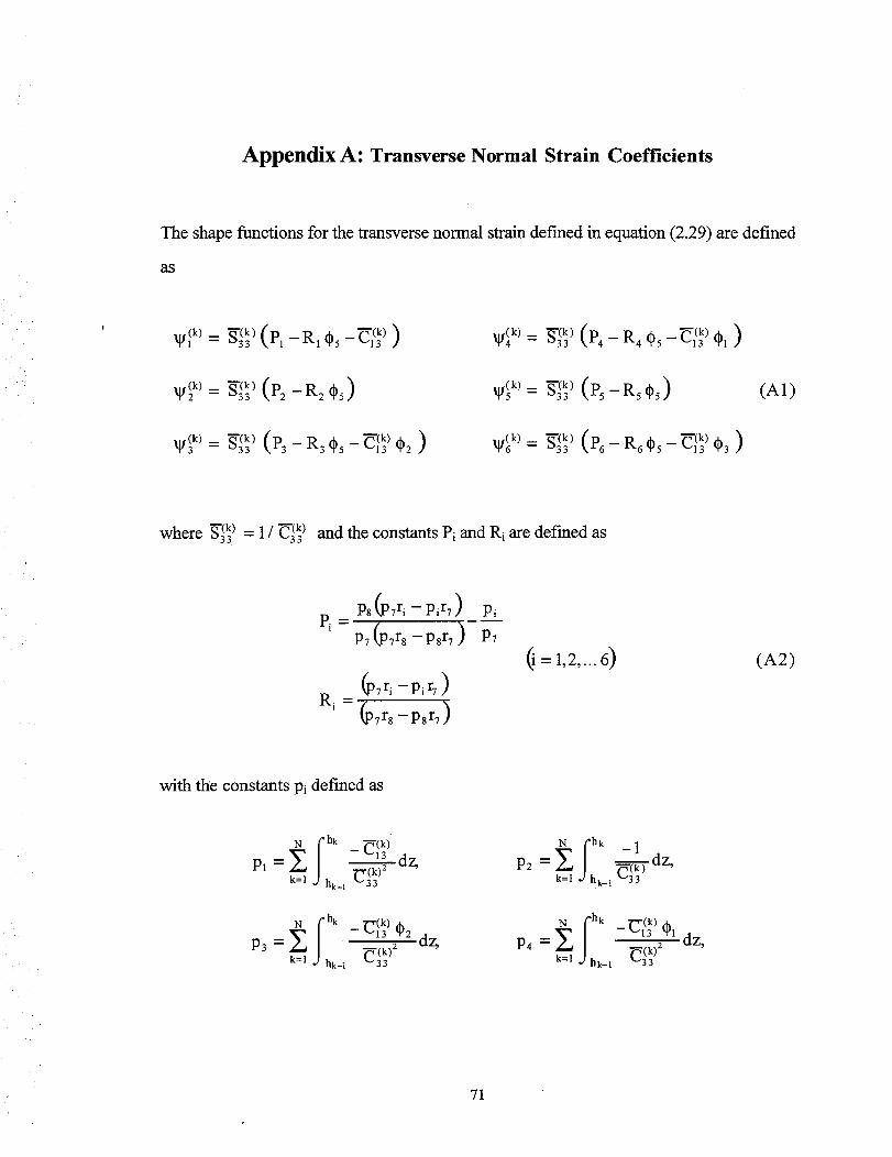
Appendix A: Transverse Normal Strain Coefficients

The shape functions for the transverse normal strain def'med in equation (2.29) are defined

as

•_k) .._ _'(k)o33 (P3 - R3 _5 _ _'(k)_13 _2 ) ll)._k, = "_'(k,.33 (P6- R6¢5 __'(k'_13 *3 )

where _'(k) = 1 / P'(k) and the constants Pi and Ri are defmed as_33 "'33

P8 (Pvri - Pir7) Pi

Pi = p7 (P7r8 _psr7 )-77

(p7ri --Pit7 )

Ri=(p7rs-psr7)

{_ = 1,2,... 6) (A2)

with the constants Pi defined as

N fhk __-(k)"-_13 dz,

Pl = _.(--_)=k= 1 hk -1 3 3

P3 =k=l hk-i _'(k)2"33 dz,

N flk -1P2 = _ _(_) dz,k=l k-I _33

fl ,,P4 = Z U(k) 2

k=l k-I 33

dz,

71

N fll -2_1_'(k)2P5 = _ dz,

k=l -1 33

P7 = Z dz,

k=l -1 33

and the ri constants are

N fh_ _'(k) 05rl = _ - "-'13 dz,

k=l Jhk_l _3(k3 )2

Z _13r 3 = _.(k)2

k=l -I "'33

r5 = _ - 2¢, O, dz,_'(k) 2

k=l k-1 33

r 7 = _ dz,

k=l k-1 33

dz,

£ fl I -- _11 k) *3P6 = _.(k)2 dz,k=l -1 "33

Ps = _ U(k)---"7"dzk=l -l 3 3

r2 = Z dz,k=l k-I

N I hk __i_(k) ¢1 ¢5Z "'13

r4 = Jhk _(k)2 dz,k=l -I 33

(k _W(k)_ 05

Jh Y3 dz,r 6 = Fr(k)2k=l k-I "33

k=l -1 33

_dz

(A3)

(A3)

72

Appendix B: Stress Resultants and Prescribed Tractions

Beam Stress Resultants:

N

Nx: bE + )dzk=l

N

N_ : b k_o 2 fhh2_,(er=llt_ k) )dzk=l

N

N H : b 2 Jhh_ (¢;(k)*2 + O',-V_ k) )dzk-1 _K--XX

k=l

N

M x = b Y_ j-dh__,(er(kx) ¢1 -]- t_zz _¢f(4 k) )dzk =1

N

M z = b k_, '_ _l__, (O_/1/; k) )dzk=l

N

MH = b Z I_'k (rCk)*3 + I_zzl_/(6k) )dzk-1 \--xx

k =1

N

Qx = b 2 _k: I,x"-(k)q_x_)dzxzk=l -1

(B1)

Prescribed Stress Resultants at Ends of Beam (@ x= 0 & x=L ) "

N N

_'xO = b Z I_h__,(Txo)dz gxL = b Z Ih__, (TxL)dZk=l k=l

N

M---xO: b 2 j'2_k_,(Txo z)dzk=l

N

Mxg : b 2 J'h"2_,(TxuZ)dzk =1

N N

M',o: bh 2 j-£h2_,(Txo,2)dz M-"1L= bh 2 Ihh__l (TxL ¢2 )dzk=l k--I

N N

M2o = b 2 j-2h__,(Txo qb3 )dz M'ZL : b 2 J'h_2_,(TxL 03 )dzk=l k =1

N N

_xO = b Z J'h_, ( Tz° )dz _-xU = b Z Ihh2, ( T_L)dzk=l - k =1 -

N N

Q,o : b Z J'2h__ 1 ( Tz0 ; )dz QIL = b Z Ihh2_,(T_L _ )dzk=l k=l

N Nhk

_%o= b Z Ihk_Tz0 (_2-- _) dz _2L = b Z Ihh2 T_L (_2-,J()dzk=l k =1

(B2)

73

Appendix C: Stiffness Coefficients for Beam Constitutive Matrix

A O.Stiffness Coefficients:

N

All = b_._k=l

N

A12 = b_k=l

N

A13 = b_k=l

N

A22= b_k =1

N

A23 = b _k=l

N

A33 = b'_k=l

C_ + 2 _3 _ + _33 _1/1 Z-!

_k (_'(k)m(k) _'(k) m(k)m(kl'_A_,k_l_13 "t'2 + _33 T1 "1"2 ]_

.f2k (_"(k, _"(k)_21l.f_k ) 4- _'(k) v_k , 4- _"(k).llf(k,_l.f_k))dzk-I _'Vll I_2 4-v13 v13 v33 el

_(k). (k)2_hk (C33 _/2 ) dZ

hk-1

f.h_ ¢¢_ ),_ ,,,_ ) "_ ) ""_),,,_) )dzk__k 13 "t'2"t'2 4- _33 %'2 "t"3

f_hkk-! _ll(_"(k)"t'2I'_2 4- 2 Ul(k' I_2 V_ k) 4- _"(k)v_k)2_33 )dz

(C1)

B O.Stiffness Coefficients:

N

Bll = b'_k=l

N

B12 = b_k=l

N

B13 = b"_k=l

N

B21 = b_k=l

N

.f__, (_kl)*l 4- C"_'¢, _g(1 k) 4- _'_k) _l.f_k) 4- _'_)l_k)v_k))dz

_(k). (k). (k) _.3_(C33 t_2 Ws }u_

74

N

B23 = b_k=l

N

B31 = b_k=l

N

B32 = b Zk=l

N

B33 = b_k=l

I_:__(_'_)qb3 _/t_k) + C'_) V_k)///_k)) dz

I_:_, (_k)¢,qb2 + _-_)_,_k) + _'_)_2_k) + _'_k) _k)_k))d z

rV,k) V,k)l,t,k)l,, k))aZ (C2)k-I t"13 *2 _k) + "'33 5"3 5"5

Ihkk, (U[kl) *2 03 q- U_k3 ) _3/l]_ k) q" U[k3 ) I[])2/11_ k) -1- U_ k) /[J_k)_/J_ k))dz

D O•Stiffness Coefficients."

N

Dll = b___,k=l

N

D12 = b_k=l

N

D13 = b_k--1

N

D22 = by_,k =I

N

D23 = b_k=l

N

D33 = b_k=l

k )_21 + 2 _13 "t'11JI/4 "[" v33 I.[J 4 Z

k-I

'k _"_"(k) _lj _k) _'(k ) ill(k) ,if (k) "_r_ 7k-1 _13 _1 "1" "'33 5°'4 "t"5 ,]_

Ih2 (_'(k) _'(k)d _ iif(k)_l__'(k)/J_ v(6k) _l_ _-r(k) l,t(k)_,t(k))dzell 0103 "t- _13 "f3 "f4 _13 "°r'l "-'33 "1"4 w6-i

_(k) (k)_

hk-I

k /'_'(k)_ lit(k) _'(k)llf(k)ilt(k)"_t.l, 7 (C3)k_l_13 _"3_1"5 -1- _33 "t"5 "t"6 ,]"_

;k (_'(k)ilf(k)2 ")_"(k)d_ _(k) _'(k)llf(k)2 )d1_11 "r3 + + z_13 "t"3 "'33 "1"6k-1

G Stiffness Coefficient:

N

G= b____I_k (_'(k)2)k-, _,_55 _x_ dzk=l

(C4)

75

./:.:'Appendix D: Derivation of Constitutive Relations

The stress-strain relations for a two-dimensional stress state are developed for plane

strain and plane stress in the x-z plane (refer to coordinate system in Figure 2.1). Both

constitutive relations are derived from the general three-dimensional state of stress and

strain for an orthotropic ply. The constitutive relations for the k th ply of a laminated

orthotropic solid are defined as

• E1 (k)

E 2

E3

723 [' =

.712Jm

-$1_ $12 $13 0 0

812 $22 $23 0 0

$13 $23 $33 0 0

0 0 0 $44 0

0 0 0 0 $55

0 0 0 0 0

0 (k)

0

0

0

0

866 m

f

!(_1 (k)

i

02

(Y3

' ,.G23 f

"_13 /

,'_12Jm

(D1)

which in condensed form are

{_m_k) = [Smlk){(_m_ k)

where the (k) superscript implies that the quantity is a function of the k th ply; [Sm] is

the conventional orthotropic compliance matrix, and the m subscript identifies the lamina

axes in the material coordinate system. The vectors { (_m } and {Em } contain stresses and

strains defined in the material reference frame.

The orthotropic plies of a laminated composite or sandwich may be of arbitrary

orientation in the x-y plane of the beam. Since the constitutive relations are given with

respect to the material coordinate system, the properties must be transformed into the

beam coordinate system. The following matrices define the stress and strain

transformations:

76

with

c2 s2 0 0 0 2cs

s2 c2 0 0 0 -2cs

0 0 1 0 0 0

0 0 0 c-s 0

0 0 0 s c 0

-cs cs 0 0 0 c2-s _

c = cos _i , s = sin13

c 2 s_ 0 0 0 cs

s2 c2 0 0 0 - cs

0 0 1 0 0 0

0 0 0 c-s 0

0 0 0 s c 0

-2cs 2cs 0 0 0 C2--S 2

(D2)

where 13 denotes the angle between the principal material direction of the ply and the x

coordinate, as depicted in Figure D. 1.

Y

2

3, z

Figure D. 1 Beam and Material Coordinate Frames

The stress and strain quantities for the material reference frame are expressed in terms

of the global (x-y coordinate) stresses and strains using the transformation matrices

defined in (D2):

{(_m _k)--[T(j.] {(_g i k) , {1_m}(k)= [Tg ] _g } k) (D3)

where the g subscript identifies quantities defined in the global coordinate system. The

equations (D3) are substituted into (D1) to yield

77

Pre multiplication of both sides of the equation by the inverse of the strain transformation

matrix results in the form

with the transformed compliance matrix defmed as

_ g]k): [TE]-I[Sm]k)[T_] (D6)

Expressing equation (D5) in expanded form yields the transformed three-dimensional

strain-stress relations in terms of global quantities:

"Ex

_y [

Ez

_/yz

_xz

_:xyJ

(k)-Sll 812 813 0 0 816"

912 822 823 0 0 826

813 823 833 0 0 836

0 0 0 844 845 0

0 0 0 S4s Sss 0

816 826 836 0 0 866

k) "Ox (k)

O'y

O" z

',Cy_F

'gxz ]

g 'gXyJg

(D7)

Although the same notation is used, the Sij coefficients shown in (D7) are not the same as

those in (D1). The coefficients from equation (D7) are derived from the transformed

compliance matrix defined in (D6) and are not expanded individually for this discussion.

78 k,

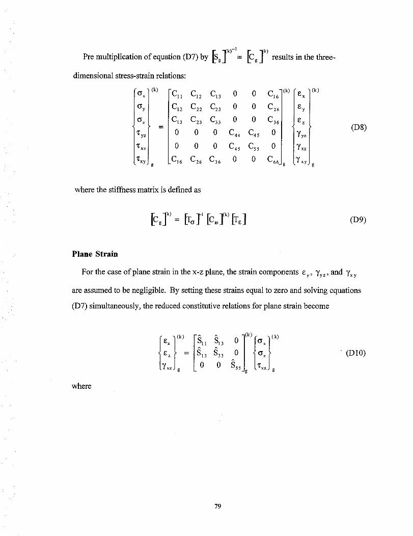
Pre multiplication of equation (D7) by [Sg ] k_-l=

dimensional stress-strain relations:

"¢_x (k)

Gy

(_z

_yz

_xz

_xy g

Cg ]k) results in the three-

[-CI1 C12 C13 0 0 C16

C12 C22 C23 0 0 C26

C13 C23 C33 0 0 C36

0 0 0 C44 C45 0

0 0 0 C45 C55 0

C16 C26 C36 0 0 C66 -

"Ex (k)

Ey

Ez

Yyz

7xz /

g )'xyJg

(D8)

where the stiffness matrix is defined as

7._k) ]-1 ](k)LX_,gj _-- [Z(_ [C m [rE] (09)

Plane Strain

For the case of plane strain in the x-z plane, the strain components ey, Yyz, and '_xy

are assumed to be negligible. By setting these strains equal to zero and solving equations

(D7) simultaneously, the reduced constitutive relations for plane strain become

where

= [s03 OzYx_ g 0 $55g a:xz g

(D10)

79

Sll "- 2S12 816826 - 8162 822 - Sll S262 -S122 S66 + Sll S22 S66

822866 - 8262

513 = 816S23S26- $262 $13 -S16 S22 S36"1-$12S26S364"$13S22S66-$12S23S66

933 _--

822866 - 8262

2S23 826S36 -822833- $22 8362 - 8232 866 q- 833822966

$22S66 - $262

(D11)

The plane strain constitutive relations can be inverted to yield the stress-strain relations:

where

/3 33o_xz _ 0 (_55_ _'xz g

$33 C13- "S_3

{_33 = _11_33_ _13 2 , _--- 95"x'7

(D12)

(D13)

Plane Stress

For a state of plane stress in the x-z plane, the stress components (_y, 'l_yz, and _xy in

equation (D8) are set equal to zero. Solving the equations in terms of the stress

components associated with x and z yields the two-dimensional constitutive relations for

plane stress:

80

where

Cll _

0 C,,Jg

2C12 C16 C26 - C162 C22 - C 11C262 - C122 C 66 --{--C 11C22 C66

C22C66 -- C262

(D14)

C13 --

_33 --

C16 C23 C26 - C262 C13 - C16 C22 C36 -Jr- C12 C26 C36 -I-- C13 C22 C66 - C12 C23C66

C22C66 - C262

2 C2s C26 C36 - C262 C33 - C22 C362 - C232 C66 -1.- C33 C22 C66

C22C66 -- C262

(D15)

i_55 = C55 -_C44

1 -_

REPORT DOCUMENTATION PAGE Form ApprovedOMB No. 0704-0188

Public reporting burden for this collection of information is estimated to average 1 hour per response, including the time for reviewing instructions, searching existing data sources,

gathering and maintaining the data needed, and completing and reviewing the collection of information. Send comments regarding this burden estimate or any other aspect of this

collection of information, including suggestions for reducing this burden, to Washington Headquarters Services. Directorate for Information Operations and Reports. 1215 Jefferson Davis

Highway, Suite 1204, Arlington, VA 22202-4302. and to the Office of Management and Budget, Paperwork Reduction Project (0704-0188), Washington, DC 20503.

1. AGENCY USE ONLY (Leave blank) 2. REPORT DATE 3. REPORTTYPE AND DATES COVERED

March 1997 Contractor Report4. TITLE AND SUBTITLE 5. FUNDING NUMBERS

A Higher-Order Bending Theory for Laminated Composite and Sandwich NCC1-208Beams 537-06-21-09

6. AUTHOR(S)

Geoffrey M. Cook

7. PERFORMING ORGANIZATION NAME(S) AND ADDRESS(ES)

George Washington UniversityJoint Institute for Advancement of Flight SciencesHampton, VA 23681-0001

:9. SPONSORING/ MONITORINGAGENCYNAME(S)ANDADDRESS(ES)

National Aeronautics and Space AdministrationLangley Research CenterHampton, VA 23681-0001

8. PERFORMING ORGANIZATIONREPORT NUMBER

10. SPONSORING/MONITORINGAGENCY REPORT NUMBER

NASA CR-201674

11. SUPPLEMENTARY NOTES

Langley Technical Monitor: Alex Tessler

12a. DISTRIBUTION/AVAILABILITY STATEMENT

Unclassified-Unlimited

Subject Category 39

12b. DISTRIBUTION CODE

13. ABSTRACT (Maximum 200 words)

A higher-order bending theory is derived for laminated composite and sandwich beams. This is accomplishedby assuming a special form for the axial and transverse displacement expansions. An independent expansion isalso assumed for the transverse normal stress. Appropriate shear correction factors based on energy

considerations are used to adjust the shear stiffness. A set of transverse normal correction factors is introduced,leading to significant improvements in the transverse normal strain and stress for laminated composite and

sandwich beams. A closed-form solution to the cylindrical elasticity solutions for a wide range of beam aspectratios and commonly used material systems. Accurate shear stresses for a wide range of laminates, includingthe challenging unsymmetric composite and sandwich laminates, are obtained using an original correctedintegration scheme. For application of the theory to a wider range of problems, guidelines for finite element

approximations are presented.

14. SUBJECTTERMS

Beam Theory; Laminated Beams; Sandwich Beams; Correction Factors;Cylindrical Bending; Interlaminar Stresses; Finite Elements; Virtual Work

17. SECURITY CLASSIFICATION

OF REPORT

Unclassified

18. SECURITY CLASSIFICATIONOF THIS PAGE

Unclassified

NSN 7540-01-280-5500

19. SECURITY CLASSIFICATIONOF ABSTRACT

Unclassified

15. NUMBER OF PAGES

88

16. PRICE CODE

A05

20. LIMITATION OF ABSTRACT

Unlimited

Standard Form 298 (Rev. 2-89)Prescribed by ANSI Std. Z39-18

298-1(_