A High Power Interior Permanent Magnet Alternator for ...
176
A High Power Interior Permanent Magnet Alternator for Automotive Applications Chong-Zhi Liaw March 15, 2013
Transcript of A High Power Interior Permanent Magnet Alternator for ...

A High Power Interior Permanent Magnet Alternator
for Automotive Applications
Chong-Zhi Liaw
March 15, 2013

Contents
Table of Contents . . . . . . . . . . . . . . . . . . . . . . . . . . . . . . . . . . . iii
List of Figures . . . . . . . . . . . . . . . . . . . . . . . . . . . . . . . . . . . . . vi
List of Tables . . . . . . . . . . . . . . . . . . . . . . . . . . . . . . . . . . . . . xii
Abstract . . . . . . . . . . . . . . . . . . . . . . . . . . . . . . . . . . . . . . . . xiii
Statement of Originality . . . . . . . . . . . . . . . . . . . . . . . . . . . . . . . xiv
Acknowledgements . . . . . . . . . . . . . . . . . . . . . . . . . . . . . . . . . . xv
Nomenclature . . . . . . . . . . . . . . . . . . . . . . . . . . . . . . . . . . . . . xvi
Abbreviations . . . . . . . . . . . . . . . . . . . . . . . . . . . . . . . . . . . . . xix
1 Introduction and Background 1
1.1 Introduction to Alternators . . . . . . . . . . . . . . . . . . . . . . . . . . 1
1.2 Trends in Power Consumption . . . . . . . . . . . . . . . . . . . . . . . . . 3
1.3 High Power Alternators . . . . . . . . . . . . . . . . . . . . . . . . . . . . . 5
1.3.1 High Power Alternator Requirements . . . . . . . . . . . . . . . . . 5
1.3.2 42V Powernet Specification . . . . . . . . . . . . . . . . . . . . . . 5
1.3.3 Load Dump Transients . . . . . . . . . . . . . . . . . . . . . . . . . 7
1.3.4 Machine Types . . . . . . . . . . . . . . . . . . . . . . . . . . . . . 7
1.3.5 Field Weakening . . . . . . . . . . . . . . . . . . . . . . . . . . . . 9
1.3.6 Power Conversion . . . . . . . . . . . . . . . . . . . . . . . . . . . . 10
1.3.7 Inverterless Alternator Concept . . . . . . . . . . . . . . . . . . . . 13
1.3.8 Recent Developments in 42 V Power Electronics and Related Work 14
1.3.9 Literature Review on Automotive Alternator Developments . . . . . 15
1.3.10 Original Contributions . . . . . . . . . . . . . . . . . . . . . . . . . 17
1.3.11 Thesis Layout . . . . . . . . . . . . . . . . . . . . . . . . . . . . . . 18
2 Interior PM Alternator Characteristics 20
2.1 Introduction to Permanent Magnet Machines . . . . . . . . . . . . . . . . . 20
iii
2.1.1 Interior PM Machine d-q Model . . . . . . . . . . . . . . . . . . . . 22
2.1.2 Generation in Interior PM Machines . . . . . . . . . . . . . . . . . 24
2.2 Uncontrolled Generation . . . . . . . . . . . . . . . . . . . . . . . . . . . . 24
2.2.1 Steady-State Model . . . . . . . . . . . . . . . . . . . . . . . . . . . 26
2.2.2 Dynamic Model . . . . . . . . . . . . . . . . . . . . . . . . . . . . . 29
2.3 Voltage-Current Loci in Uncontrolled Generation . . . . . . . . . . . . . . 29
2.3.1 Saliency Ratio . . . . . . . . . . . . . . . . . . . . . . . . . . . . . . 31
2.3.2 Stator Resistance . . . . . . . . . . . . . . . . . . . . . . . . . . . . 32
2.3.3 Magnetic Saturation . . . . . . . . . . . . . . . . . . . . . . . . . . 36
2.4 Stator Current Hysteresis . . . . . . . . . . . . . . . . . . . . . . . . . . . 36
2.4.1 Hysteresis explained using VI Loci . . . . . . . . . . . . . . . . . . 38
2.5 Experimental Investigation . . . . . . . . . . . . . . . . . . . . . . . . . . . 40
2.5.1 Test Machine Parameters and Construction . . . . . . . . . . . . . 41
2.5.2 Experimental Setup . . . . . . . . . . . . . . . . . . . . . . . . . . . 42
2.5.3 Short-Circuit Test . . . . . . . . . . . . . . . . . . . . . . . . . . . . 45
2.5.4 Three-Phase Resistive Load Test . . . . . . . . . . . . . . . . . . . 47
2.5.5 Generation into a Rectifier and Resistive Load . . . . . . . . . . . . 49
2.5.6 Generation into a Rectifier and Voltage Source Load . . . . . . . . 53
2.6 Summary of Findings . . . . . . . . . . . . . . . . . . . . . . . . . . . . . . 57
3 Switched-Mode Rectifier Control 61
3.1 Introduction to Switched Mode Rectification . . . . . . . . . . . . . . . . . 61
3.2 SMR Operation . . . . . . . . . . . . . . . . . . . . . . . . . . . . . . . . . 63
3.3 SMR Modelling . . . . . . . . . . . . . . . . . . . . . . . . . . . . . . . . . 65
3.4 Experimental Setup . . . . . . . . . . . . . . . . . . . . . . . . . . . . . . . 69
3.5 Open-Loop System Response . . . . . . . . . . . . . . . . . . . . . . . . . 72
3.5.1 Voltage and Current Waveforms . . . . . . . . . . . . . . . . . . . . 72
3.5.2 Steady-State Output Current Response . . . . . . . . . . . . . . . . 73
3.5.3 Output Power and Efficiency . . . . . . . . . . . . . . . . . . . . . . 74
3.5.4 Dynamic Duty-Cycle Response . . . . . . . . . . . . . . . . . . . . 79
3.6 Controller Design and Implementation . . . . . . . . . . . . . . . . . . . . 82
3.6.1 Limits of Stability . . . . . . . . . . . . . . . . . . . . . . . . . . . 83
3.6.2 Simulation . . . . . . . . . . . . . . . . . . . . . . . . . . . . . . . . 87
3.7 Closed-Loop System Response . . . . . . . . . . . . . . . . . . . . . . . . . 88
3.7.1 Steady-State Voltage Regulation . . . . . . . . . . . . . . . . . . . . 88
iv

3.7.2 Transient Voltage Regulation . . . . . . . . . . . . . . . . . . . . . 89
3.8 Summary of Findings . . . . . . . . . . . . . . . . . . . . . . . . . . . . . . 91
4 Idle-Speed Power Improvement 93
4.1 Introduction . . . . . . . . . . . . . . . . . . . . . . . . . . . . . . . . . . . 93
4.2 Power Converters . . . . . . . . . . . . . . . . . . . . . . . . . . . . . . . . 95
4.2.1 Single-Switch SMR and Inverter Low-Speed Performance . . . . . . 95
4.2.2 Proposed Semi-Bridge SMR Modulation Scheme . . . . . . . . . . . 96
4.3 Simulation Studies . . . . . . . . . . . . . . . . . . . . . . . . . . . . . . . 98
4.3.1 Inverter Control versus Conventional SMR Control . . . . . . . . . 99
4.3.2 SMR Modulation Strategy . . . . . . . . . . . . . . . . . . . . . . . 103
4.3.3 Optimal Operating Regions . . . . . . . . . . . . . . . . . . . . . . 107
4.4 Experimental Setup . . . . . . . . . . . . . . . . . . . . . . . . . . . . . . . 109
4.5 Experimental Results . . . . . . . . . . . . . . . . . . . . . . . . . . . . . . 112
4.6 Summary of Findings . . . . . . . . . . . . . . . . . . . . . . . . . . . . . . 114
5 Conclusions 116
5.1 Background . . . . . . . . . . . . . . . . . . . . . . . . . . . . . . . . . . . 116
5.2 Original Contributions . . . . . . . . . . . . . . . . . . . . . . . . . . . . . 117
5.3 Interior PM Machine Generation Characteristics . . . . . . . . . . . . . . . 118
5.4 Switched-Mode Rectifier Control . . . . . . . . . . . . . . . . . . . . . . . 120
5.5 Summary . . . . . . . . . . . . . . . . . . . . . . . . . . . . . . . . . . . . 124
5.5.1 Further Work . . . . . . . . . . . . . . . . . . . . . . . . . . . . . . 125
Bibliography 131
Appendices 132
A Publications 132
B Programs 166
B.1 Matlab and Simulink Code . . . . . . . . . . . . . . . . . . . . . . . . . . . 166
B.2 Microcontroller Code . . . . . . . . . . . . . . . . . . . . . . . . . . . . . . 172
B.2.1 Closed-Loop Control . . . . . . . . . . . . . . . . . . . . . . . . . . 172
B.2.2 Low-Speed Power Improvement . . . . . . . . . . . . . . . . . . . . 179
v

List of Figures
1.1 Power generation, storage and usage in an automotive electrical system . . 1
1.2 Simplified diagram of a conventional Lundell alternator . . . . . . . . . . . 2
1.3 Graph of historical and projected electrical demand in cars . . . . . . . . . 4
1.4 High power alternator specification, showing power and efficiency require-
ments . . . . . . . . . . . . . . . . . . . . . . . . . . . . . . . . . . . . . . 6
1.5 Operating voltage limits for the 42V Powernet specification . . . . . . . . . 7
1.6 Comparison of power vs. speed curves achieved by various types of electri-
cal machines . . . . . . . . . . . . . . . . . . . . . . . . . . . . . . . . . . . 8
1.7 Machine parameters under field-weakening operation . . . . . . . . . . . . 10
1.8 AC machines operating with various power converter circuits . . . . . . . . 12
1.9 Output power obtained from a Lundell alternator using different power
converter configurations . . . . . . . . . . . . . . . . . . . . . . . . . . . . 12
1.10 Interior PM alternator with inverter and inverterless circuit configurations 13
2.1 Cross-sections of a surface PM and an interior PM machine . . . . . . . . . 21
2.2 Equivalent circuit model for a surface PM machine . . . . . . . . . . . . . 22
2.3 Interior PM machine rotor indicating synchronous d-q frame axes and pha-
sor diagram of currents and voltages during operation . . . . . . . . . . . . 22
2.4 Equivalent circuits for an interior PM machine in the d-axis and the q-axis 23
2.5 Equivalent circuits for uncontrolled generation . . . . . . . . . . . . . . . . 24
2.6 Phasor diagram for an interior PM machine operating into a resistive load 26
2.7 D and q-axis inductance curves for varying levels of magnetic saturation, βn 28
2.8 Single-phase equivalent circuit of an electrical machine modelled as a volt-
age source with series impedance while operating into a resistive load . . . 30
2.9 Voltage-current loci for DC, surface PM and interior PM machines . . . . . 30
vi

2.10 Normalised voltage-current loci for various saliency ratios ξ, neglecting the
effects of stator resistance and saturation. . . . . . . . . . . . . . . . . . . 32
2.11 Voltage overshoot versus saliency ratio ξ, neglecting the effects of stator
resistance and saturation . . . . . . . . . . . . . . . . . . . . . . . . . . . . 33
2.12 Ideal voltage-current loci at various speeds ωen for saliency ratio ξ = 6,
Rph = 0 pu . . . . . . . . . . . . . . . . . . . . . . . . . . . . . . . . . . . 33
2.13 Normalised voltage-current loci for various values of normalised stator re-
sistance Rn, with ξ = 6 . . . . . . . . . . . . . . . . . . . . . . . . . . . . . 34
2.14 Normalised voltage-current loci at various speeds ωen, with Rn = 0.42 pu
at base speed . . . . . . . . . . . . . . . . . . . . . . . . . . . . . . . . . . 35
2.15 Open-circuit voltage and maximum voltage vs. machine speed for various
values of stator resistance Rn, with ξ = 6 . . . . . . . . . . . . . . . . . . . 35
2.16 Voltage overshoot versus Rn for various values of saliency ratio ξ, showing
the locations of the two test machines based on their unsaturated saliency
ratio and normalised stator resistance at 1,500 rpm . . . . . . . . . . . . . 36
2.17 Normalised voltage-current loci for various values of saturation parameter
βn, with Rn = 0 and ξ = 6 . . . . . . . . . . . . . . . . . . . . . . . . . . . 37
2.18 Typical stator current vs. speed characteristic of an interior PM machine
exhibiting hysteresis . . . . . . . . . . . . . . . . . . . . . . . . . . . . . . 37
2.19 The relationship between the VI loci and the stator current vs. speed
characteristic of an interior PM machine exhibiting hysteresis . . . . . . . . 39
2.20 Hysteresis versus DC link voltage for various values of Rn, with ξ = 6 . . . 40
2.21 Rotor cross-sections for the multiple-barrier and axially-laminated machines 41
2.22 Multiple-barrier rotor with rare-earth magnets . . . . . . . . . . . . . . . . 41
2.23 Measured d-axis and q-axis inductance saturation curves for the multiple-
barrier and axially-laminated machines . . . . . . . . . . . . . . . . . . . . 43
2.24 Dynamometer rig test setup for testing the interior PM alternator . . . . . 44
2.25 Variable gearbox for the dynamometer rig . . . . . . . . . . . . . . . . . . 44
2.26 Short-circuit phase current and torque vs. speed for the multiple-barrier
machine . . . . . . . . . . . . . . . . . . . . . . . . . . . . . . . . . . . . . 45
2.27 Short-circuit phase current and torque vs. speed for the axially-laminated
machine . . . . . . . . . . . . . . . . . . . . . . . . . . . . . . . . . . . . . 46
2.28 Voltage-current loci for the multiple-barrier machine, operating at 1,500 rpm
with a three-phase resistive load, showing the effect of non-idealities . . . . 48
vii
2.29 Voltage-current loci for the axially-laminated machine, operating at 1,500 rpm
with a three-phase resistive load, showing the effect of non-idealities . . . . 48
2.30 AC VI and VP loci for the multiple-barrier machine at various speeds . . . 49
2.31 DC VI and VP loci for the multiple-barrier machine at various speeds . . . 50
2.32 AC VI and VP loci for the axially-laminated machine at various speeds . . 51
2.33 DC VI and VP loci for the axially-laminated machine at various speeds . . 52
2.34 Predicted rectified open-circuit and maximum voltage vs. machine speed . 53
2.35 Model predictions and measured hysteresis band as a function of the DC
link voltage for the axially-laminated machine . . . . . . . . . . . . . . . . 54
2.36 Model predictions and measured hysteresis band as a function of the DC
link voltage for the multiple-barrier machine . . . . . . . . . . . . . . . . . 55
2.37 Calculated and measured UCG stator current characteristic with speed for
the multiple-barrier machine operating into a 110V DC voltage source . . . 56
2.38 Calculated and measured UCG stator current characteristic with speed for
the axially-laminated machine operating into a 40V DC voltage source . . 57
2.39 Enlarged view of the hysteresis band shown in Fig. 2.32 . . . . . . . . . . . 58
2.40 Measured vs. simulated stator current and voltage waveforms in UCG for
the multiple-barrier machine . . . . . . . . . . . . . . . . . . . . . . . . . . 59
3.1 AC machines operating with various power converter circuits . . . . . . . . 62
3.2 Interior PM alternator operating with an SMR into a DC voltage source load 63
3.3 The effect of switched-mode rectifier operation on the alternator stator line
voltage waveform and effective DC link voltage seen by the alternator . . . 64
3.4 Comparison of the operation of an uncontrolled rectifier and a switched-
mode rectifier . . . . . . . . . . . . . . . . . . . . . . . . . . . . . . . . . . 64
3.5 Duty-cycle control of alternator output current with the alternator operat-
ing as a constant current source at high speeds . . . . . . . . . . . . . . . . 65
3.6 Calculated scaling effect of duty-cycle on interior PM alternator VI locus . 66
3.7 Calculated scaling effect of duty-cycle on alternator input and output current 66
3.8 Contour plot of calculated DC output current vs. duty-cycle and alternator
speed for a 200 V DC link voltage. . . . . . . . . . . . . . . . . . . . . . . 67
3.9 Contour plot of calculated machine efficiency (%) vs. duty-cycle and alter-
nator speed for a 200 V DC link voltage. . . . . . . . . . . . . . . . . . . . 68
3.10 Three-phase inverter used as a switched-mode rectifier . . . . . . . . . . . 69
3.11 Experimental configuration for open-loop SMR testing . . . . . . . . . . . 70
viii
3.12 d-axis and q-axis inductance saturation curves for the interior PM alterna-
tor with 135 V stator obtained by scaling the 415 V stator measurements . 71
3.13 135 V alternator short-circuit current and torque vs. speed . . . . . . . . . 72
3.14 Calculated alternator DC VI and VP loci at various speeds, with experi-
mental points for 1,800 and 3,000 rpm . . . . . . . . . . . . . . . . . . . . 73
3.15 Measured waveforms illustrating the effect of 50% duty-cycle SMR switch-
ing on the stator voltage and current . . . . . . . . . . . . . . . . . . . . . 74
3.16 DC input and output currents vs. duty-cycle at various speeds, with a
200 V DC link voltage . . . . . . . . . . . . . . . . . . . . . . . . . . . . . 75
3.17 Measured SMR DC input and DC output current versus duty-cycle from
the alternator operating at 6,000 rpm plotted against ideal curves . . . . . 75
3.18 Measured alternator open-circuit and short-circuit iron and mechanical
losses with speed . . . . . . . . . . . . . . . . . . . . . . . . . . . . . . . . 77
3.19 Alternator efficiency vs. DC output power for various alternator speeds,
showing steady-state model predictions neglecting iron loss and measured
results . . . . . . . . . . . . . . . . . . . . . . . . . . . . . . . . . . . . . . 77
3.20 Alternator efficiency vs. DC output power for various alternator speeds,
showing steady-state model predictions incorporating iron loss . . . . . . . 78
3.21 Alternator maximum generating output power, input torque, duty-cycle
and efficiency vs. speed, showing steady-state model predictions and mea-
sured results, for a 200 V DC link voltage . . . . . . . . . . . . . . . . . . 79
3.22 Calculated DC output current vs. duty cycle at 1,800 rpm for various DC
link voltages, with measured current for a 50 V DC link. . . . . . . . . . . 80
3.23 Duty-cycle command with a frequency of 200 Hz and corresponding alter-
nator output current waveform (averaged signals shown) . . . . . . . . . . 81
3.24 Measured open-loop frequency response and fitted curves for the alternator
and SMR at 1,800 rpm with a 50 V DC link voltage . . . . . . . . . . . . . 81
3.25 Calculated and measured dynamic response of the DC output current to
step changes in switching duty-cycle at 1,800 rpm . . . . . . . . . . . . . . 83
3.26 System diagram of the closed-loop system with a proportional controller . 83
3.27 Linear control law for the controller, for various values of proportional gain,
Kp . . . . . . . . . . . . . . . . . . . . . . . . . . . . . . . . . . . . . . . . 84
3.28 Calculated open-loop frequency response of the interior PM alternator and
SMR, showing gain and phase margins . . . . . . . . . . . . . . . . . . . . 85
ix

3.29 Calculated discrete root locus plot of the open-loop system with a sampling
period of 284 µs . . . . . . . . . . . . . . . . . . . . . . . . . . . . . . . . . 86
3.30 Enlarged view showing root loci for various values of sampling time Ts,
with values of proportional gain shown at various points on the locus for
sampling time Ts = 284 µs . . . . . . . . . . . . . . . . . . . . . . . . . . . 86
3.31 Measured duty-cycle and DC link voltage during 50 V regulation at 1,500 rpm,
at load currents of 5.5, 18.4 and 27.2 A . . . . . . . . . . . . . . . . . . . . 88
3.32 Measured duty-cycle and DC link voltage during 100 V regulation at 1,500 rpm,
with a 6.0 Ω load . . . . . . . . . . . . . . . . . . . . . . . . . . . . . . . . 89
3.33 Closed-loop voltage regulation vs. load current at 1,500 rpm, for DC link
voltages of 50, 100, 150 and 200 V . . . . . . . . . . . . . . . . . . . . . . . 90
3.34 Experimental configuration for closed-loop load dump tests . . . . . . . . . 90
3.35 Simulated and measured duty-cycle and DC link voltage waveforms show-
ing the load-dump response of the closed-loop system operating at 1,800 rpm
with a 100 V DC link . . . . . . . . . . . . . . . . . . . . . . . . . . . . . . 91
4.1 Output power versus speed characteristics for an example Lundell and in-
terior PM alternator using different power electronics topologies . . . . . . 94
4.2 Comparison of SMR and inverter operation: the SMR acts as a resistive
load with fixed unity power factor while the inverter produces a controllable
power-factor allowing it to extract more power at low speeds . . . . . . . . 97
4.3 Three-phase parallel resistance and capacitance per phase used to produce
the ”inverter” maximum output power characteristics . . . . . . . . . . . . 98
4.4 Diagram illustrating modulation scheme intervals in relation to phase cur-
rent and effective voltage . . . . . . . . . . . . . . . . . . . . . . . . . . . . 99
4.5 Relationship between phase currents, phase effective voltage and gate drive
signals for the new modulation scheme . . . . . . . . . . . . . . . . . . . . 100
4.6 Calculated d-q current plane operating trajectories for the SMR and the
inverter with or without a voltage limit, operating at 1800 rpm with a DC
link voltage of 200 V . . . . . . . . . . . . . . . . . . . . . . . . . . . . . . 101
4.7 Calculated output power versus phase current for the SMR and the inverter
with and without voltage limit . . . . . . . . . . . . . . . . . . . . . . . . . 101
4.8 Calculated phase voltage versus phase current for the SMR and the inverter
with and without voltage limit . . . . . . . . . . . . . . . . . . . . . . . . . 102
x
4.9 Calculated power factor versus phase current for the SMR and the inverter
with and without voltage limit . . . . . . . . . . . . . . . . . . . . . . . . . 102
4.10 Contour plot of calculated rms phase current versus modulation parameters
δ and ε at 1,800 rpm, showing operating points of interest . . . . . . . . . 104
4.11 Contour plot of calculated average output power (kW) versus modulation
parameters δ and ε at 1,800 rpm . . . . . . . . . . . . . . . . . . . . . . . . 105
4.12 Conventional SMR ’load-matching’ operation at point C (δ = 0, ε = 180) 106
4.13 Short-circuit operation at point A (δ = 180, ε = 0) . . . . . . . . . . . . 106
4.14 Maximum phase current obtained at point D (δ = 105, ε = 5) . . . . . . 107
4.15 Maximum power obtained at point E (δ = 60, ε = 0) . . . . . . . . . . . 107
4.16 Maximum power obtained with rated current at point F (δ = 45, ε = 5) . 108
4.17 Scatter plot of calculated feasible d-q currents available using the proposed
SMR modulation scheme at 1,800 rpm, with key operating points indicated 109
4.18 Scatter plot of calculated output power versus phase current at 1,800 rpm
with key operating points indicated . . . . . . . . . . . . . . . . . . . . . . 110
4.19 Experimental configuration for low-speed power improvement testing . . . 110
4.20 Measured phase current and effective voltage for 1,800 rpm generation into
a 200 V load while operating in load-matching at point C (δ = 0, ε = 180)112
4.21 Measured phase current (upper trace) and effective voltage (inverted gate
drive signal) (lower trace) for 1,800 rpm generation into a 200 V load while
operating at point F (δ = 45, ε = 5) . . . . . . . . . . . . . . . . . . . . . 113
4.22 Operation at point F, as in Fig. 4.21, except with voltage levels of Vδ =
40 V and Vφ = 160 V . . . . . . . . . . . . . . . . . . . . . . . . . . . . . . 114
5.1 Output power versus speed characteristics for the interior PM alternator
compared against high power alternator power specifications . . . . . . . . 125
xi

List of Tables
1.1 Existing high-power alternator research categorised by machine and type
of power electronics . . . . . . . . . . . . . . . . . . . . . . . . . . . . . . . 17
2.1 Measured test machines parameters . . . . . . . . . . . . . . . . . . . . . . 42
3.1 Interior PM alternator parameters with 415 V and 135 V stators . . . . . . 71
xii

Abstract
This thesis examines the operation of a 6 kW interior permanent magnet machine as
a generator and its use in conjunction with a switched-mode rectifier as a controllable
current source. The interior permanent magnet machine was designed for optimum field-
weakening performance which allows it to achieve a wide constant-power speed range.
This configuration has possible applications in power generation, e.g. as an alternator in
automotive electrical systems and in renewable energy systems such as small-scale wind
turbines.
The thesis starts from a study of the behaviour of the interior PM machine while
generating into a three-phase resistive load and also through a rectifier into a voltage
source load. Steady-state and dynamic d-q models are developed which describe the ma-
chine generation characteristics. The concept of the VI locus is introduced which provides
insights into the generating performance of interior PM machines. In particular, the phe-
nomenon of hysteresis in the current versus speed characteristic of highly salient interior
PM machines is explained using the VI locus and for the first time is experimentally
demonstrated.
The steady-state and transient response of the 6 kW interior PM machine while op-
erating with a switched-mode rectifier is modeled and experimentally measured, forming
the basis for the design of a closed-loop controller to regulate the output voltage. The
experimental performance and stability of the closed-loop system is examined and eval-
uated. Further improvements to the output power of the system at low speed using a
switched-mode rectifier modulation scheme are investigated and a 66% improvement in
output power from 2.8 kW to 4.7 kW is experimentally demonstrated.
xiii

Statement of Originality
I, Chong-Zhi Liaw certify that this work contains no material which has been accepted for
the award of any other degree or diploma in any university or other tertiary institution
and, to the best of my knowledge and belief, contains no material previously published
or written by another person, except where due reference has been made in the text.
I give consent to this copy of my thesis when deposited in the University Library, being
made available for loan and photocopying, subject to the provisions of the Copyright Act
1968.
I also give permission for the digital version of my thesis to be made available on
the web, via the University’s digital research repository, the Library catalogue and also
through web search engines, unless permission has been granted by the University to
restrict access for a period of time.
Signed:
Date:
xiv

Acknowledgements
I would like to offer my deepest gratitude to my supervisor, Associate Prof. Wen L. Soong
for his invaluable guidance, patience and support throughout the course of my research,
as well as to my co-supervisor Associate Prof. Nesimi Ertugrul for his valued feedback
and advice.
I would also like to thank the staff of the University of Adelaide Electrical Engineering
Workshop for their assistance with my laboratory work as well as my fellow colleagues
with whom I have had the pleasure of collaborating, in particular Dr. David Whaley and
Dr. Vlatka Zivotic-Kukolj.
I would like to thank my family for their faith in me and lastly my wife, June for her
endless support and encouragement.
This thesis was supported by Australian Research Council Discovery Grant DP0342874.
xv

Nomenclature
βn normalised magnetic saturation parameter
δ the angle between the back-emf E and the output voltage Vo of an electrical machine
ωe electrical frequency
Ψm magnet flux linkage
ξ saliency ratio of an interior PM machine
C DC link capacitance
d PWM duty-cycle
E induced back-EMF of an electrical machine
Gm gain margin of a transfer function
Id d-axis current
id time-varying d-axis current
If field current in an alternator winding
Iq q-axis current
iq time-varying q-axis current
IIN DC current before the SMR switch
ILOAD current delivered to a load
IOUT DC current after the SMR switch
Iqn normalised q-axis current
xvi

ISW DC current flowing through the SMR switch to ground
Kp proportional gain of a closed-loop controller
Ld d-axis inductance
Lq q-axis inductance
Ldn normalised d-axis inductance
Lqno normalised unsaturated q-axis inductance
Lqn normalised q-axis inductance
RL load resistance
Rn normalised resistance
RS stator resistance
RT total resistance
Rph stator resistance of an electrical machine
T reaction torque of an electrical machine
Ts sampling time of a closed-loop controller
Vd d-axis voltage
vd time-varying d-axis voltage
Vo open-circuit voltage of an electrical machine
Vo output voltage
Vq q-axis voltage
vq time-varying q-axis voltage
Vs line voltage of an electrical machine
VDC DC link voltage
VEFF effective voltage seen at the terminals of an electrical machine
xvii

Vmax maximum voltage obtained on a voltage-current locus
Xd d-axis reactance
Xq q-axis reactance
ZS source impedance
xviii

Abbreviations
AC Alternating Current
CPSR Constant Power Speed Ratio
DC Direct Current
FET Field Effect Transistor
LCD Liquid Crystal Display
PWM Pulse-Width Modulation
SAE Society of Automotive Engineers
SLI Starting, Lighting and Ignition
SMR Switched-Mode Rectifier
UCG Uncontrolled Generation
VI Voltage-Current
xix

Chapter 1
Introduction and Background
1.1 Introduction to Alternators
An alternator is a device that converts mechanical energy to alternating electrical current.
The term normally refers to the small Alternating Current (AC) generators found in
automotive vehicles, where mechanical energy is supplied by a combustion engine. In
these vehicles, the alternator is usually coupled via a belt system to the engine drive
shaft and generates electricity both to charge the battery of the vehicle and to supply
electrical loads, most importantly for engine Starting, Lighting and Ignition (SLI) but
also including air-conditioning, heating, pumps, wiper motors and various other on-board
systems (see Fig. 1.1) [1].
Battery Electrical LoadsRecti!erAlternator
Starter
Motor
Fuel
Pump
Compressor On-Board
Electronics
Figure 1.1: Power generation, storage and usage in an automotive electrical system
The alternator was first developed in the 19th century by pioneers such as Michael
Faraday and Nikola Tesla. The first large-scale introduction of alternators in cars was
1

CHAPTER 1. INTRODUCTION AND BACKGROUND
to replace the Direct Current (DC) generators previously used for powering the vehicle
electrical system. While various improvements to the alternator have since been made, its
basic design remains unchanged. The most commonly used modern alternator topology
is known as the Lundell alternator (see Fig. 1.2), which is a three-phase, wound-field
synchronous machine of a simple claw-pole rotor design with an integrated rectifier and
regulator. The steel claw-pole design of the Lundell alternator is mechanically robust and
can be cheaply manufactured. A reasonable amount of maintenance is required, usually
due to wear of brushes and slip rings. The Lundell alternator produces 1-2 kW of output
power and achieves approximately 50% efficiency from shaft to output [1].
Stator RectifierClaw-Pole
Rotor
Figure 1.2: Simplified diagram of a conventional Lundell alternator
As with other AC generators, alternators work via the principle of electromagnetic
induction. Mechanical power input to the alternator causes the rotor to turn relative to
the stator. As the magnetic field of the rotor cuts across the stationary windings of the
stator, an alternating voltage is induced. In the Lundell alternator, a field current, If is
fed via slip rings and brushes to the rotor to produce its magnetic field.
The induced AC output voltage of the alternator is proportional to both the strength
of the rotor magnetic field and the alternator speed. By changing the value of field current,
the magnitude of the output voltage, Vs can be controlled. This is shown in (1.1), where
the alternator speed is represented in terms of its electrical angular frequency, ωe. The
alternator three-phase output voltage is converted by an integrated bridge rectifier to DC,
which is required by the electrical loads in a car.
Vs ∝ ωeif (1.1)
2

CHAPTER 1. INTRODUCTION AND BACKGROUND
The output voltage of the alternator is kept constant by the integrated regulator which
monitors the output voltage and adjusts the current in the field winding to increase
or decrease the magnetic field of the rotor and thus control the output voltage (1.1).
The presence of the car battery as a load also helps to absorb any voltage ripples or
disturbances such as load changes caused by other electrical devices in the car being
turned on or off.
An alternator is faced with the task of providing sufficient output power to supply the
electrical accessory loads over the entire operating speed range of the car engine. This
typically ranges from an idle speed of 600 rpm to a top speed of 6,000 rpm and since the
alternator output power is generally proportional to speed, producing sufficient power at
low speeds is particularly challenging. Alternators are therefore commonly run with a
belt ratio of 3:1 to obtain a higher rotational speed of 1,800 rpm at engine idle.
The surplus power generated by the alternator is used to maintain the battery charge
level. This is important because when the engine is not running, any active devices must
draw their power from the battery alone, e.g. the starter motor used to crank the engine.
A typical consumer vehicle has a 12 V lead-acid battery and the alternator output is
slightly higher at 14 V in order to provide a suitable charging voltage. The battery
generally has a capacity of around 80 Ah and may be called upon to supply currents as
large as 200 A for engine cranking.
Ideally, an alternator should maximise output power and efficiency while minimising
the cost of manufacture and maintenance. Mounted near the engine of a vehicle, the
alternator is exposed to constant vibration and high temperatures, thereby reducing its
performance and lifetime.
1.2 Trends in Power Consumption
The demand for electrical power in vehicles has been steadily rising, as shown in Fig. 1.3.
With the conventional Lundell alternator limited to 1-2 kW of output power, newer vehi-
cles are already approaching the limits of the Lundell alternator’s capability. The graph
of Fig. 1.3 was published in 2000 and shows the projected electrical power demand in cars
up to 2005.
The increase in power demand has largely been driven by the plethora of new features
being introduced into vehicles to provide increased performance, safety and comfort. Some
of these applications, such as active suspension and electromechanical valve timing, re-
3
CHAPTER 1. INTRODUCTION AND BACKGROUND
Figure 1.3: Graph of historical and projected electrical demand in cars [2], and breakdownof electrical demand in generic luxury vehicles in 1996 and 2005 [3]
quire large currents in order to achieve the desired mechanical effect. Active suspension
involves using actuators to actively control the suspension system of a vehicle in order
to enhance the smoothness of travel or even adjust the grip of the vehicle on the road
surface. Electromechanical valve timing describes the replacement of the mechanical cam
shafts used to control engine valves by electrical actuators, allowing the valve timing to
be fully and dynamically controlled in order to optimise fuel efficiency and engine power
in varying conditions.
A further contributing factor to increased electrical power demand is the gradual
replacement of engine-driven devices such as water pumps, air-conditioning compressors
and power-steering pumps with electrical alternatives. This relieves the mechanical load
on the engine and reduces maintenance needed by moving parts such as belts and drive
clutches. This change also results in greater fuel efficiency, particularly for devices which
see intermittent use, e.g. an air-conditioning compressor.
Apart from improvements to the basic functionality of the vehicle, various auxiliary
on-board systems are also becoming increasingly popular and affordable, such as satellite
navigation, video entertainment systems and even small inverters to power mains-voltage
appliances such as laptop computers. These ever-increasing demands to be placed on
the next generation of automotive electrical systems highlight the need for a high-power
successor to the Lundell alternator.
4
A NOTE: These figures/tables/images have been removed to comply with copyright regulations. It is included in the print copy of the thesis held by the University of Adelaide Library.
CHAPTER 1. INTRODUCTION AND BACKGROUND
1.3 High Power Alternators
1.3.1 High Power Alternator Requirements
In the mid to late 1990s, the Massachusetts Institute of Technology (MIT)/Industry
Consortium on Advanced Automotive Electrical/Electronic Components and Systems [4]
provided several recommendations in an effort to formulate and standardise solutions for
addressing the high power demands of future vehicles. The main points can be summarised
as follows:
• More power - output power ranging from 4 kW at engine idle speed (600 rpm) to
6 kW at top speed (6,000 rpm), corresponding approximately to a constant power
speed range of 10:1
• Better efficiency - a requirement of 75% system efficiency at 75% load at 1,500 rpm
engine speed (4,500 rpm alternator speed assuming a 3:1 pulley ratio)
• Higher and better regulated output voltage - strict voltage limits around a 42 V
output voltage as specified by the 42V Powernet specification
The requirements for output power and efficiency are considerably higher than those
achieved by a conventional Lundell alternator and are illustrated in Fig. 1.4. A useful met-
ric relevant to this output power requirement is the constant power speed range (CPSR)
of a machine, which is the range of operating speed over which a machine is capable of
producing rated power. If the rated speed is defined as the speed at which rated power and
torque are produced, the CPSR is expressed as the ratio of the maximum speed at which
rated power is obtainable to the rated speed. The high power alternator specification is
approximately equivalent to a CPSR ratio of 10:1.
1.3.2 42V Powernet Specification
The shift from the existing 14 V electrical system voltage to a 42 V system, as rec-
ommended by the Consortium, represents a significant development in the automotive
industry. The preceding shift from 7 V to 14 V did not entail such an extensive change to
the electrical system because the only electrical loads present at the time were for start-
ing, lighting and ignition, whereas electrical devices are now pervasive in modern vehicles.
The main reason for this move is to improve the efficiency of the electrical system - the
three-fold increase in system voltage allows a three-fold reduction of the current required
5

CHAPTER 1. INTRODUCTION AND BACKGROUND
0 2 4 6 8 10 12 14 16 180
2
4
6
Alternator Speed [krpm]
Out
put P
ower
[kW
]
High Power Specification
Lundell Alternator
75% efficiency at 75% load at 4,500 rpm
Figure 1.4: High power alternator specification, showing power and efficiency require-ments
to deliver the equivalent power to car loads. This results in a nine-fold reduction in copper
losses alone, which is especially important at the higher levels of output power specified.
Originally an initiative of Mercedes Benz and the Massachussets Institute of Technol-
ogy, the next-generation automotive electrical system based on a 42 V system voltage
is formalised in the Society of Automotive Engineers (SAE) 42V Powernet specification.
The operating voltage of 42 V was originally chosen because it was the highest possible
multiple of 14 V which satisfied the internationally established safe peak voltage limit of
60 V while allowing a reasonable voltage margin for transients. By offering reduced I2R
transmission losses, the higher operating voltage also allows the use of lighter wiring and
insulation. The resulting weight reduction also translates to savings in fuel.
The 42 V specification enforces strict voltage regulation (see Fig. 1.5), reducing the
need for device over-rating and thus leading to cost savings at the component level. The
overall savings can be significant - it is estimated that the cost of an automotive electrical
system exceeds that of the engine and transmission combined and that the electrical
wiring harness typically makes up more than 35 kg of a vehicle’s weight [5].
Some issues remain to be addressed in the adoption of the 42 V standard. One of
these is the increased risk of arcing at the high levels of voltage involved and another
is the problem of jump-starting [6]. Dual 12 V and 42 V rail systems have also been
investigated in order to ensure compatibility with existing 12 V lighting and accessories
while the industry transitions to the new standard [7].
6

CHAPTER 1. INTRODUCTION AND BACKGROUND
0 21 30 42 50 58 Low voltage limit for loads related to safety
Lower operating limit for all other loads
Nominal engine running voltage
Maximum steady-state overvoltage (including ripple)
Maximum transient overvoltage (load dump)
Figure 1.5: Operating voltage limits for the 42V Powernet specification
1.3.3 Load Dump Transients
Although the integrated regulator of an alternator monitors its output voltage, the car’s
electrical system may still experience large disturbances in certain extreme situations,
such as when the connection to the battery is lost while the alternator is running. With-
out the battery to absorb the generated power, the alternator voltage climbs sharply. The
regulator employs field current control to regulate the output voltage and thus cannot re-
spond instantaneously - the inductance of the field winding prevents the field current from
changing quickly. This condition is known as a load dump and the associated transient
voltage peak can be as large as 80 V and last for hundreds of milliseconds [8, 9].
In order to cope with the voltage transient, electrical components throughout the car
must be over-rated to withstand voltages much higher than the operating voltage. As
more higher power devices are incorporated into vehicles, the cost of the necessary device
over-rating grows. The introduction of more sophisticated and sensitive electronics also
means that the power quality of the car’s electrical supply becomes increasingly important
in a next-generation vehicle.
1.3.4 Machine Types
Research into viable high power automotive alternators has turned to various types of elec-
trical machines, including other wound-field synchronous machines, induction machines
(IM), switched reluctance machines, surface permanent magnet (SPM) and interior per-
manent magnet (IPM) machines. The performance achieved in early studies with these
machines is summarised in Fig. 1.6, with the curve for the conventional Lundell alternator
shown for reference.
While it would be possible to scale an existing 14 V wound-field Lundell alternator for
7

CHAPTER 1. INTRODUCTION AND BACKGROUND
0 2 4 6 8 10 12 14 16 180
1
2
3
4
5
6
7
High Power Specification
Lundell 14V
IM 42V [8]
IM 42V [7]
SPM 42V [10]
IPM Machine [1]
Alternator Speed [krpm]
Out
put P
ower
[kW
]
Figure 1.6: Comparison of power vs. speed curves achieved by various types of electricalmachines
42 V output by tripling the number of winding turns in the stator, this would not change
its output power.
The asynchronous or induction machine is very widely used in industrial applications
and has the benefit of being robust and relatively inexpensive. Work on induction ma-
chines as automotive alternators has achieved maximum output powers of around 4 kW,
however this power tends to fall off at engine speeds beyond 4 krpm [10, 11, 12] (see
Fig. 1.6).
The switched and variable reluctance machines are attractive because of their sim-
ple construction and high efficiency. Their inert rotors without windings or magnets are
inexpensive and robust, making them suitable for operation at high speed and in high tem-
perature conditions [13]. However, they do suffer from significant torque ripple, vibration
and noise.
Permanent magnet (PM) machines have also attracted significant interest in alternator
applications. As the rotor magnetic field is provided by magnets instead of field windings,
PM machines offer high efficiency and power density which allow for a more compact
design.
8

CHAPTER 1. INTRODUCTION AND BACKGROUND
Although improvements in manufacturing have helped reduce the cost of permanent
magnets, it is worth noting that in recent years, the price of rare-earth magnet materials
has risen by over an order of magnitude. This has been due to reduced supply and tighter
export limitations imposed by China since 2005, which at the time supplied more than
90% of the global rare-earth metal demand. While there has been a ramping up of rare-
earth production in other countries as well as increased pressure on China to loosen export
controls, this situation remains an economic concern for permanent magnet applications.
1.3.5 Field Weakening
As shown in Fig. 1.6, one of the main challenges faced has been that of meeting the output
power requirement specification - the output power of the machine must be maintained
above the specification line for all engine speeds from 600 rpm to 6,000 rpm (see Fig. 1.4),
i.e. the machine must deliver rated voltage and current over that operating speed range.
The back-emf of electrical machines is proportional to the product of the speed and
the flux in the machine. In machines where the flux is relatively constant, such as surface
PM machines, it is difficult to operate above rated speed without exceeding the rated
output voltage. This could be solved by employing a DC-to-DC converter to maintain a
constant output voltage. However, at top speed the power electronic components in the
converter would be required to withstand both rated current (150 A, for 6 kW at 42 V)
and the considerable machine back-emf of several hundred volts. This approach therefore
involves increased power electronics cost and complexity.
Another method to maintain rated voltage is to reduce the flux in the machine, as
for example in the Lundell alternator, where this is accomplished by reducing the field
current and thus the magnetic field of the rotor (see (1.1)). Figure 1.7 shows how if
at above rated speed the alternator terminal voltage and armature current are kept at
rated values and the field current is decreased inversely proportionally to the speed, the
torque likewise decreases with 1/ωe. The output power, being the product of torque and
speed, thus remains constant. Operating at above rated speeds in this fashion is known
as field-weakening and makes it theoretically possible to achieve a very high Constant
Power Speed Ratio (CPSR).
A study by Schiferl and Lipo showed that interior PM machines offer the best field-
weakening performance of any AC synchronous machine and thus have the potential to
achieve a wide CPSR [14]. This study also described the optimal field-weakening condition
for interior PM machines (1.2), where the magnet flux-linkage Ψm is equal to the d-axis
9

CHAPTER 1. INTRODUCTION AND BACKGROUND
0 0.5 1 1.5 2 2.5 30
0.5
1
1.5o
utp
ut
torq
ue
0 0.5 1 1.5 2 2.5 30
0.5
1
1.5
ou
tpu
t p
ow
er
0 0.5 1 1.5 2 2.5 30
0.5
1
1.5
inp
ut
vo
lta
ge
0 0.5 1 1.5 2 2.5 30
0.5
1
1.5
sta
tor
cu
rre
nt
0 0.5 1 1.5 2 2.5 30
0.5
1
1.5
mo
tor
flu
x
speed [pu]
rated speed
Figure 1.7: Machine parameters under field-weakening operation
stator inductance Ld multiplied by the rated stator current Io.
Ψm = LdIo (1.2)
1.3.6 Power Conversion
The three-phase AC output of an alternator must be converted to a DC current suitable
for charging the battery of a vehicle. Several circuit configurations which are capable of
achieving this are shown in Fig. 1.8.
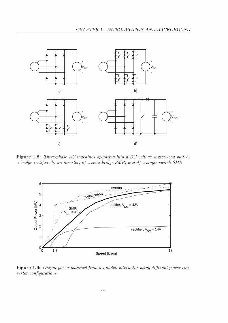
The simplest means of producing a DC output is the three-phase bridge rectifier (see
10
CHAPTER 1. INTRODUCTION AND BACKGROUND
Fig. 1.8.a) and this is the configuration commonly used in conventional automotive alter-
nators. If the DC link voltage of the rectifier is increased by a factor of three from 14 V
to 42 V then this would increase the output power at high speeds by a factor of three as
shown in Fig. 1.9. It would however also increase the speed at which generation starts by
a factor of three and reduce the idle speed output power to zero.
The configuration which delivers the most power at any speed from an alternator
is an inverter (see Fig. 1.8.b). An inverter has two independently controlled switches
per phase-leg which can be used to modify the phase and amplitude of the current and
voltage waveforms in order to extract maximum power from the machine. This provides
maximum power transfer but at the cost of additional power electronics switches and a
more complex control system.
Semi-bridge (see Fig. 1.8.c) and single-switch (see Fig. 1.8.d) Switched-Mode Recti-
fiers (SMRs) represent intermediate steps between the inverter and the bridge rectifier.
Previous work by Perreault has investigated the use of a Lundell alternator with a semi-
bridge switched-mode rectifier in place of a bridge rectifier [9]. By modulating the SMR
switches with a Pulse-Width Modulation (PWM) signal of controllable duty, the effective
load voltage seen by the alternator could be manipulated in order to obtain power at all
speeds. Later work by Rivas examined a phase advance SMR modulation scheme which
could improve Lundell alternator output power at idle speed [15].
The various power converter topologies will be discussed in more detail in later chapters
but the output power obtained from a Lundell alternator with each configuration is shown
in Fig. 1.9 for the purpose of comparison.
11
CHAPTER 1. INTRODUCTION AND BACKGROUND
VDC
+
-
VDC
+
-
a) b)
VDC
+
-
VDC
+
-
c) d)
Figure 1.8: Three-phase AC machines operating into a DC voltage source load via: a)a bridge rectifier, b) an inverter, c) a semi-bridge SMR, and d) a single-switch SMR
0 1.8 180
1
2
3
4
5
6
Speed [krpm]
Out
put P
ower
[kW
]
rectifier, VDC
= 14V
rectifier, VDC
= 42V SMR
VDC
= 42V
inverter
specification
Figure 1.9: Output power obtained from a Lundell alternator using different power con-verter configurations
12
CHAPTER 1. INTRODUCTION AND BACKGROUND
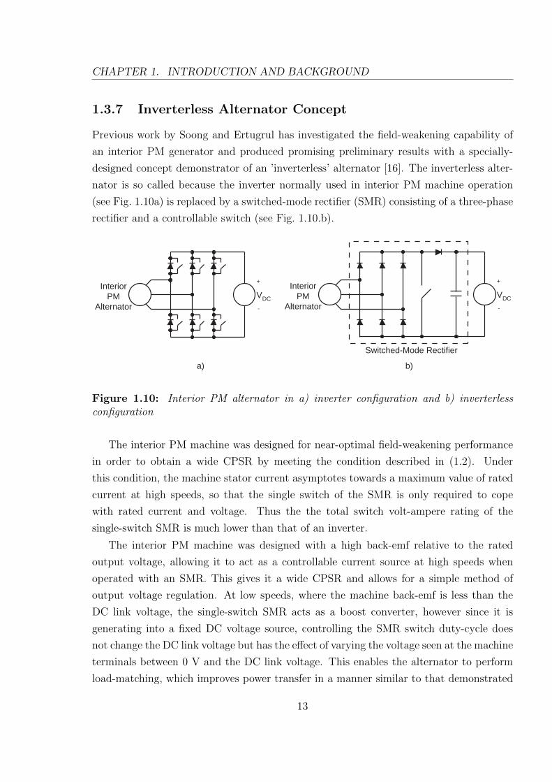
1.3.7 Inverterless Alternator Concept
Previous work by Soong and Ertugrul has investigated the field-weakening capability of
an interior PM generator and produced promising preliminary results with a specially-
designed concept demonstrator of an ’inverterless’ alternator [16]. The inverterless alter-
nator is so called because the inverter normally used in interior PM machine operation
(see Fig. 1.10a) is replaced by a switched-mode rectifier (SMR) consisting of a three-phase
rectifier and a controllable switch (see Fig. 1.10.b).
InteriorPM
Alternator
Switched-Mode Rectifier
VDC
+
-
InteriorPM
AlternatorVDC
+
-
a) b)
Figure 1.10: Interior PM alternator in a) inverter configuration and b) inverterlessconfiguration
The interior PM machine was designed for near-optimal field-weakening performance
in order to obtain a wide CPSR by meeting the condition described in (1.2). Under
this condition, the machine stator current asymptotes towards a maximum value of rated
current at high speeds, so that the single switch of the SMR is only required to cope
with rated current and voltage. Thus the the total switch volt-ampere rating of the
single-switch SMR is much lower than that of an inverter.
The interior PM machine was designed with a high back-emf relative to the rated
output voltage, allowing it to act as a controllable current source at high speeds when
operated with an SMR. This gives it a wide CPSR and allows for a simple method of
output voltage regulation. At low speeds, where the machine back-emf is less than the
DC link voltage, the single-switch SMR acts as a boost converter, however since it is
generating into a fixed DC voltage source, controlling the SMR switch duty-cycle does
not change the DC link voltage but has the effect of varying the voltage seen at the machine
terminals between 0 V and the DC link voltage. This enables the alternator to perform
load-matching, which improves power transfer in a manner similar to that demonstrated
13

CHAPTER 1. INTRODUCTION AND BACKGROUND
by Perreault in his work with a Lundell alternator [9]. Although this configuration uses
two less switches and one more diode than the semi-bridge rectifier in Perreault’s study,
the effect of the switching is similar, since Perreault used a single control signal for all
three SMR switches.
The inverterless interior PM alternator offers a wide CPSR, obtained using fewer
switches and simpler control as compared to an inverter. As position sensors are not
necessary and lower switch VA ratings are allowed, the cost of this configuration is further
reduced. Preliminary studies with the interior PM machine using a variable three-phase
resistive load to simulate load-matching performance showed promising results, achieving
more than 6 kW of power at 4 krpm (see Fig. 1.6) [16].
1.3.8 Recent Developments in 42 V Power Electronics and Re-
lated Work
The majority of the work in this thesis (2003-7) was carried out at a time of significant
interest in the 42 V automotive electrical system specification. However, as of 2012, there
has been only limited commercial adoption of this standard and some in the industry are
of the opinion that 42 V is no longer on the horizon [17].
In part, this has been due to vehicle and component manufacturers weighing the
long-term benefits of a higher system voltage against the immediate cost and time re-
quired to redevelop the extensive and well-established 14 V infrastructure. With heavy
economic pressure in many countries, vehicle makers may be more inclined to reduce
commercial risk by investing in projects which result in an immediate, obvious benefit
to consumers. Some of this focus has gone into the development of hybrid and electric
vehicles, for which there is a growing market in the face of increasing petroleum prices.
The integrated starter/alternator, which has been one of the major applications of a 42 V
electrical bus and intended to improve fuel economy, is already employed in several cur-
rent hybrid-electric vehicles; for instance, the Hybrid Synergy Drive in the Toyota Prius,
which operates with a 200 V battery pack and uses an inverter to raise the voltage to
650 V DC to drive the electric motor [18].
Other reasons given for the difficulty in adopting the 42 V standard include problems
with the lack of standardisation of 42 V connectors, safety issues with test and repair of
42 V systems in the field and reduced reliability of 42 V components. The latter is due
to the larger arcs and subsequent contact erosion occurring in switches and relays under
the higher voltage which thus requires a redesign of these components to improve their
14

CHAPTER 1. INTRODUCTION AND BACKGROUND
reliability [19].
Such issues are not insurmountable given sufficient incentive, however this must be
accomplished “within realistic R&D budgets that reflect the economics of our times”
[20]. On the one side, we have hybrid-electric vehicles such as Toyota’s Prius, which have
already moved ahead with a higher voltage bus and battery to cater for increased power
demand, while using a DC/DC converter to charge a separate 12 V battery and power
existing 14 V accessories. On the other side, some of the electrical issues to be addressed
by the 42 V standard such as growing wiring losses and weight have been somewhat
mitigated by manufacturers using techniques such as wire multiplexing, and some of the
features previously requiring more power such as electrical power steering can now operate
properly under 14 V as a result of ongoing development [17].
Considering the many benefits of a higher voltage architecture, some see the move to a
higher standard voltage as only being put off for a time by advances in other areas. Whilst
any prediction regarding the fate of the 42 V standard would be speculation, the standard
does continue to act as a common focus for research efforts, with many of the outcomes
being potentially scalable and applicable regardless of the standard the industry eventually
adopts. A brief look at recent publications reveals continuing and varied research [21,
22, 23, 24, 25, 26] into 42 V alternators and associated power converters, which will be
discussed in the following section.
1.3.9 Literature Review on Automotive Alternator Developments
In this subsection a brief outline is provided of the range of existing research conducted
with the aim towards developing alternator technology with suitable output power, effi-
ciency and cost-effectiveness for 42 V automotive applications. Specifically, the scope of
this thesis in relation to the existing research is summarised in Table 1.1, in terms of the
type of machine and power electronics used.
• Henry et al. [11] implemented a prototype belt-driven induction machine starter-
generator for 42 V systems, utilising an inverter. This system was capable of pro-
ducing an output power of approximately 4 kW, however at higher speeds this was
reduced, e.g. to 2 kW at 4,000 rpm. The overall efficiency of the alternator and the
power electronics was between 73% and 79%.
• Naidu et al. [10] constructed a surface PM alternator with a single SCR bridge
rectifier being used to regulate the output voltage, producing 3.4 kW of output
15

CHAPTER 1. INTRODUCTION AND BACKGROUND
power up to 6,500 rpm, with 71% full-load efficiency at that speed.
• Carrichi et al. [27] constructed a 3 kW surface PM starter-alternator using Litz
wire winding to reduce winding losses and thus improve efficiency at higher speeds.
An inverter was used as the power converter and a full-load efficiency of 96% was
achieved at 3,000 rpm.
• Liang et al. [28] employed six-step inverter control with a Lundell alternator and
obtained a 43% increase in output power at idle speed.
• Lovelace et al. [29] found that the major factor in the cost of the alternator and
power electronics was in fact the cost of the inverter. This highlights a benefit of
employing a switched-mode rectifier as opposed to the more complex and costly
inverter.
• Perreault et al. [9] investigated the application of half-bridge SMR control to a
Lundell alternator in order to extract more power through load-matching. Load-
matching allowed the output power of the alternator to increase linearly from 1 kW
at an idle speed of 1,800 rpm to approximately 4 kW at 6,000 rpm whereas with a
conventional diode rectifier the output power would be limited to 1.5 kW.
• Rivas et al. [15] introduced a phase advance SMR modulation scheme to increase
the output power of a Lundell alternator power at idle speed. This scheme was
implemented with a half-bridge SMR and produced a 15% increase in output power
at idle speed.
In the time since the work in this thesis was carried out, there have been further
related studies, as follows:
• Shrud et al. [21] developed an analytical model and simulated the performance of a
42 V Lundell alternator and rectifier system.
• Stoia et al. [22] investigated the design parameters of a 42 V Lundell alternator for
use with an integrated single-switch SMR.
• Mudannayake et al. [23] investigated the performance of a 42 V integrated starter/al-
ternator (ISA) based on a 5.5 kW induction machine, implementing stator voltage
control with an inverter to extract more output power at high speeds and regulate
output voltage.
16
CHAPTER 1. INTRODUCTION AND BACKGROUND
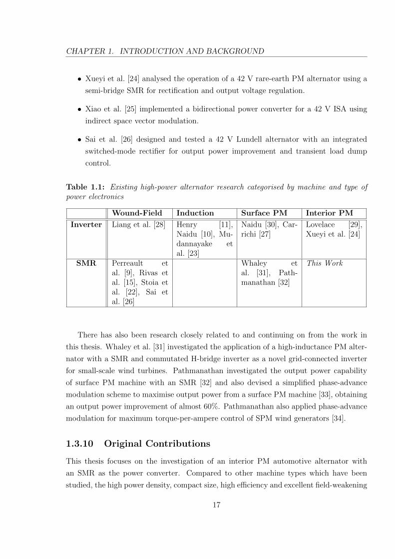
• Xueyi et al. [24] analysed the operation of a 42 V rare-earth PM alternator using a
semi-bridge SMR for rectification and output voltage regulation.
• Xiao et al. [25] implemented a bidirectional power converter for a 42 V ISA using
indirect space vector modulation.
• Sai et al. [26] designed and tested a 42 V Lundell alternator with an integrated
switched-mode rectifier for output power improvement and transient load dump
control.
Table 1.1: Existing high-power alternator research categorised by machine and type ofpower electronics
Wound-Field Induction Surface PM Interior PM
Inverter Liang et al. [28] Henry [11],Naidu [10], Mu-dannayake etal. [23]
Naidu [30], Car-richi [27]
Lovelace [29],Xueyi et al. [24]
SMR Perreault etal. [9], Rivas etal. [15], Stoia etal. [22], Sai etal. [26]
Whaley etal. [31], Path-manathan [32]
This Work
There has also been research closely related to and continuing on from the work in
this thesis. Whaley et al. [31] investigated the application of a high-inductance PM alter-
nator with a SMR and commutated H-bridge inverter as a novel grid-connected inverter
for small-scale wind turbines. Pathmanathan investigated the output power capability
of surface PM machine with an SMR [32] and also devised a simplified phase-advance
modulation scheme to maximise output power from a surface PM machine [33], obtaining
an output power improvement of almost 60%. Pathmanathan also applied phase-advance
modulation for maximum torque-per-ampere control of SPM wind generators [34].
1.3.10 Original Contributions
This thesis focuses on the investigation of an interior PM automotive alternator with
an SMR as the power converter. Compared to other machine types which have been
studied, the high power density, compact size, high efficiency and excellent field-weakening
17

CHAPTER 1. INTRODUCTION AND BACKGROUND
performance of the interior PM machine makes it a promising candidate for development
as a next-generation, high power automotive alternator with a wide CPSR.
The key contributions of this work are summarised as follows:
• Analysis of the generation characteristics of the interior PM machine when operating
into a resistive/voltage source load, including the development of steady-state and
dynamic models capable of predicting the machine output.
• Introduction of the VI locus as a tool in the steady-state modelling of electrical
machines and its application to modelling the effects of saliency, magnetic saturation
and stator resistance on interior PM alternators and in particular the hysteresis in
the output current.
• Experimental validation of the developed models, including output current hys-
teresis in an interior PM machine, which has not previously been experimentally
demonstrated.
• Investigation and modelling of SMR-based control of the interior PM machine
output and experimental demonstration of alternator output power maximisation
through load-matching. Demonstration of closed-loop voltage regulation and tran-
sient suppression using the SMR.
• Dynamic modelling of a phase-advance modulation scheme to improve the output
power of the interior PM alternator at idle speed. Implementation and testing of
the phase-advance modulation scheme on a microcontroller.
1.3.11 Thesis Layout
This thesis is divided into several chapters which examine different aspects of the interior
PM machine relevant to this application:
• Chapter 2 covers the fundamental theory governing the generation characteristics
of PM machines and discusses several interesting aspects particular to interior PM
machines, such as saliency and voltage overshoot.
• Chapter 3 investigates the behaviour of the interior PM machine when a SMR is
employed to control the output power. A simple closed-loop controller is examined
to evaluate the performance of the alternator as a regulated voltage source.
18

CHAPTER 1. INTRODUCTION AND BACKGROUND
• Chapter 4 investigates the use of a phase advance SMR modulation technique to
improve the output power of the alternator at idle speed, thereby allowing it to
meet the 42V high power alternator output power specification.
• Chapter 5 summarises the key findings and original contributions of this work and
outlines areas of potential for further investigation.
19
Chapter 2
Interior PM Alternator
Characteristics
This chapter examines the operating principles of the interior permanent magnet machine
in its function as an alternator. The behaviour of the interior PM machine during gener-
ation operation is analysed, in particular the case of generation into a DC voltage source
load.
The concept of the Voltage-Current (VI) locus is introduced to illustrate the behaviour
of the interior PM machine in this operating mode, with attention to the phenomenon
of stator current hysteresis. Theoretical models are developed for both steady-state and
dynamic situations in order to predict the currents and voltages present in the interior
PM machine, taking into account the effects of saliency, DC link voltage and non-idealities
such as magnetic saturation and stator resistance. Lastly, experimental results from two
different test machines are presented and compared against theoretical predictions.
2.1 Introduction to Permanent Magnet Machines
A brushless permanent magnet machine is a form of synchronous AC machine in which
the magnetising flux of the rotor is supplied by permanent magnets rather than a field
winding. They are generally divided into surface PM and interior PM machines, the latter
being distinguished by having magnets embedded inside the rotor, rather than mounted
on the rotor surface (see Fig. 2.1).
Some of the general advantages of brushless PM machines over other machine types
are their high efficiency and power density and therefore attractiveness in applications
20

CHAPTER 2. INTERIOR PM ALTERNATOR CHARACTERISTICS
Surface PM Interior PM
Figure 2.1: Cross-sections of a surface PM and an interior PM machine
requiring compact size. Since the flux is provided by permanent magnets, machine ex-
citation losses are eliminated. On the other hand, PM machines are susceptible to de-
magnetisation if the magnetic field generated by the stator winding currents become too
high. This can be prevented by avoiding excessive stator currents during operation.
One of the main reasons for using an interior PM machine as an alternator in this
study is its good field-weakening performance. This gives the interior PM machine an
advantage over the surface PM machine as it is then easier to achieve a high CPSR - one
of the requirements implicit in the high power alternator specification. Additionally, the
interior PM machine torque has contributions from both magnet and reluctance torque,
allowing a higher torque density.
A surface PM machine can be modelled as the machine back-emf voltage, E in series
with the synchronous inductance, Ls and resistance, Rs (see Fig. 2.2). Ls is the inductance
of the path taken by magnetic flux within the machine due to the stator current, which in
the case of the surface PM machine can be considered to be constant for all rotor angles,
as the magnets mounted on the rotor surface have a permeability close to that of air. The
synchronous inductance is relatively small due to the large electromagnetic airgap.
In an interior PM machine, however, the path taken by the flux is complicated by the
presence of the magnets embedded in the rotor. The characteristics of the interior PM
machine are accordingly more complex and are described in this chapter as the d-q model
of the interior PM machine is examined.
21

CHAPTER 2. INTERIOR PM ALTERNATOR CHARACTERISTICS
V E
I LSRS
Figure 2.2: Equivalent circuit model for a surface PM machine
d-axis
q-axis ω LdId
Id
Iq
I
ω LqIq
E = ωψm
θ γ
d-axis
q-axis
VIRs
Figure 2.3: Interior PM machine rotor indicating synchronous d-q frame axes and pha-sor diagram of currents and voltages during operation (the effect of stator resistance isneglected)
2.1.1 Interior PM Machine d-q Model
The synchronous d-q model defines flux flowing in two orthogonal axes in the rotor frame
of reference - the direct or d-axis and the quadrature or q-axis, as indicated in Fig. 2.3.
The q-axis flux follows a path through the solid body of the rotor which in most cases
is made of steel, whereas the d-axis flux path passes through the magnets in the rotor.
The magnet flux linkage, Ψm lies in the positive d-axis and thus the induced back-emf,
E = ωeΨm appears in the positive q-axis.
The steady-state phase equations for the d and q-axis voltages Vd and Vq of the d-q
model can be derived from the phasor diagram of Fig. 2.3.
Vq = RsIq + ωeLdId + ωΨm (2.1)
22

CHAPTER 2. INTERIOR PM ALTERNATOR CHARACTERISTICS
Vd = RsId − ωeLqIq (2.2)
Output torque, T =3
2p (ΨmIq − (Lq − Ld)IdIq)
where p = number of pole-pairs(2.3)
In contrast with the surface PM machine, the inductance in the d- and q-axes differ.
The magnetic permeability of the magnets is close to that of air and thus the effective
air-gap in the d-axis is larger than in the q-axis. As a result, the q-axis inductance, Lq is
higher than the d-axis inductance, Ld.
The ratio of the q-axis inductance to the d-axis inductance is known as the saliency
ratio ξ = Lq/Ld and is an important parameter which determines the field-weakening
performance and torque characteristics of the machine. The saliency in the rotor causes
a reluctance torque proportional to (Lq − Ld) to be produced, in a similar fashion to
a synchronous reluctance machine. This reluctance torque is in addition to the magnet
alignment torque, together comprising the total output torque in interior PM machines,
from (2.3).
As the stator current flowing in an interior PM machine is increased, the magnetic flux
flowing through the stator and rotor iron increases and at some point begins to saturate.
Saturation can reduce both the d and q-axis inductances at higher operating currents.
This reduction is less evident in the d-axis due to the larger effective airgap.
Vq
Iq RS
ωLdId ωψm
Lq
q-axis circuitd-axis circuit
Vd
Id RS
ωLqIq
Ld
Figure 2.4: Equivalent circuits for an interior PM machine in the d-axis and the q-axis
The d- and q-axis equivalent circuits for an interior PM machine corresponding to
23
CHAPTER 2. INTERIOR PM ALTERNATOR CHARACTERISTICS
(2.1) and (2.2) are given in Fig. 2.4, where the controlled voltage sources represent the
interaction between the d-axis and q-axis circuits.
2.1.2 Generation in Interior PM Machines
Although interior PM machines have recently experienced increased popularity in motor-
ing applications because of their efficiency and compact size, their use as generators has
been limited. This is partly because unlike the wound-field Lundell alternator, there is
no direct control of the magnetic flux being provided by the magnets in a PM machine
and therefore in order to control the voltage or current output of an interior PM machine
and maximise its power transfer to a load, additional power electronics is needed.
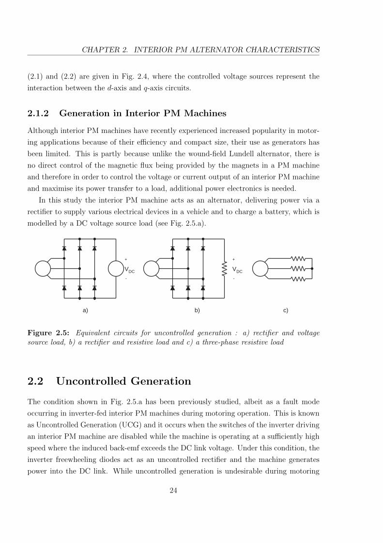
In this study the interior PM machine acts as an alternator, delivering power via a
rectifier to supply various electrical devices in a vehicle and to charge a battery, which is
modelled by a DC voltage source load (see Fig. 2.5.a).
VDC
+
-
b) c)
VDC
+
-
a)
Figure 2.5: Equivalent circuits for uncontrolled generation : a) rectifier and voltagesource load, b) a rectifier and resistive load and c) a three-phase resistive load
2.2 Uncontrolled Generation
The condition shown in Fig. 2.5.a has been previously studied, albeit as a fault mode
occurring in inverter-fed interior PM machines during motoring operation. This is known
as Uncontrolled Generation (UCG) and it occurs when the switches of the inverter driving
an interior PM machine are disabled while the machine is operating at a sufficiently high
speed where the induced back-emf exceeds the DC link voltage. Under this condition, the
inverter freewheeling diodes act as an uncontrolled rectifier and the machine generates
power into the DC link. While uncontrolled generation is undesirable during motoring
24

CHAPTER 2. INTERIOR PM ALTERNATOR CHARACTERISTICS
operation, it can be seen from Fig. 2.5.a that this is essentially the same configuration as
when an interior PM alternator provides power to a DC voltage source load such as a car
battery.
The fault currents generated during UCG operation can be undesirably large in mo-
toring applications and hence an early investigation by Adnanes concerned the calculation
of these fault current magnitudes in PM machines [35]. In the case of Adnanes’ study,
the fault currents involved were large because of the low inductance and hence high short-
circuit current of the interior PM machines investigated.
In order to theoretically model the fault currents in UCG, the voltage source load
of Fig. 2.5.a can be simplified to an equivalent resistance, giving a rectifier and resistive
load (see Fig. 2.5.b). This can be further simplified using the findings of Caliskan [36],
who analysed three-phase rectifiers with a constant voltage load and an ac-side reactance,
which in the case of UCG is the machine inductance. Caliskan’s study offered a simplified
analysis based on the assumptions that:
• the machine phase currents are balanced, sinusoidal and free of harmonics during
operation;
• the rectifier forces the phase currents to be strictly in phase with the phase voltages
(viewed from the generator convention).
Caliskan showed that almost all of the real power is transmitted to the voltage source
load in the fundamental of the phase current waveform. Provided the above assumptions
are valid, the rectifier and voltage source load can be approximated by a three-phase
resistive load (see Fig. 2.5.c).
While the first assumption is generally valid over most of the speeds of interest for the
machines used in this study, it may not hold at very low machine speeds where the phase
currents tend to become non-sinusoidal. The second assumption is a known property of
waveforms in a rectifier.
Further investigations into UCG included a more detailed theoretical analysis and
steady-state modeling of UCG in interior PM machines by Jahns [37], which takes into
account magnetic saturation but assumes zero stator resistance. This model also predicts
a hysteresis effect for high saliency machines. A study into fault modes of PM machines
by Welchko [38] also introduced a time-stepping dynamic d-q model which takes into
consideration various transient effects.
25

CHAPTER 2. INTERIOR PM ALTERNATOR CHARACTERISTICS
2.2.1 Steady-State Model
jI qX q
jI qX q
jIXq
jId X
d
jId X
q
Iq
I d
Vco
sδ
δ
Isinδ
I
V = Vo+IR
S
Vo = IR
LV
o
Eo
d-axis
q-a
xis
V
IRS
Figure 2.6: Phasor diagram for an interior PM machine operating into a resistive load
The currents and voltages in an interior PM machine operating in UCG can be rep-
resented by the phasor diagram in Fig. 2.6, which corresponds to equations (2.1) and
(2.2).
The standard method for analysing salient-pole synchronous generators starts from
knowledge of the magnitudes of the output voltage V and the output current I, as well as
the phase difference between V and I. From these, the magnitude of the induced voltage
E0 and the rotor angle δ between E0 and V can be determined from equation 2.4.
δ = 6 (V + jIXq), hence E0 = V cos δ + IdXd
where the d-axis current component Id = I sin δ(2.4)
26
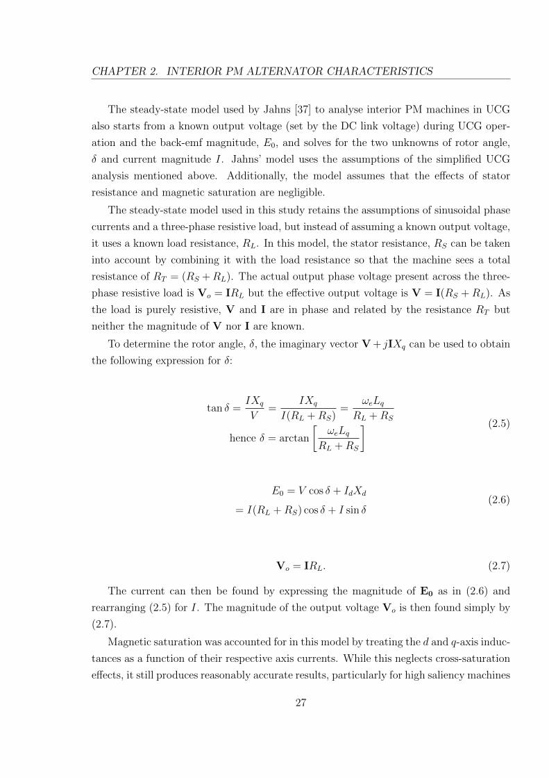
CHAPTER 2. INTERIOR PM ALTERNATOR CHARACTERISTICS
The steady-state model used by Jahns [37] to analyse interior PM machines in UCG
also starts from a known output voltage (set by the DC link voltage) during UCG oper-
ation and the back-emf magnitude, E0, and solves for the two unknowns of rotor angle,
δ and current magnitude I. Jahns’ model uses the assumptions of the simplified UCG
analysis mentioned above. Additionally, the model assumes that the effects of stator
resistance and magnetic saturation are negligible.
The steady-state model used in this study retains the assumptions of sinusoidal phase
currents and a three-phase resistive load, but instead of assuming a known output voltage,
it uses a known load resistance, RL. In this model, the stator resistance, RS can be taken
into account by combining it with the load resistance so that the machine sees a total
resistance of RT = (RS +RL). The actual output phase voltage present across the three-
phase resistive load is Vo = IRL but the effective output voltage is V = I(RS +RL). As
the load is purely resistive, V and I are in phase and related by the resistance RT but
neither the magnitude of V nor I are known.
To determine the rotor angle, δ, the imaginary vector V + jIXq can be used to obtain
the following expression for δ:
tan δ =IXq
V=
IXq
I(RL +RS)=
ωeLqRL +RS
hence δ = arctan
[ωeLq
RL +RS
] (2.5)
E0 = V cos δ + IdXd
= I(RL +RS) cos δ + I sin δ(2.6)
Vo = IRL. (2.7)
The current can then be found by expressing the magnitude of E0 as in (2.6) and
rearranging (2.5) for I. The magnitude of the output voltage Vo is then found simply by
(2.7).
Magnetic saturation was accounted for in this model by treating the d and q-axis induc-
tances as a function of their respective axis currents. While this neglects cross-saturation
effects, it still produces reasonably accurate results, particularly for high saliency machines
27

CHAPTER 2. INTERIOR PM ALTERNATOR CHARACTERISTICS
such as those considered in this study. The functions Ld(Id) and Lq(Iq) are obtained from
experimental inductance measurements of the machines used in this study. A spline curve
fit to the data was used to provide values to the simulation, which iterates until the values
of inductance converge.
An approximate normalised non-linear parametric model of magnetic saturation was
developed by Jahns [37] based on experimental data, and this will be used in later sections
to examine the effect of saturation without being machine specific. This model is described
by (2.8), where Lqno is the unsaturated value of Lqn when Iqn is zero, and βn determines
the degree to which Lqn is affected by saturation as illustrated in Fig. 2.7. This model
assumes that the value of Ldn is constant with respect to Idn and thus unaffected by
saturation.
Lqn = Ldn +(Lqno − Ldn)
[1 + (βnIqn)2]1/2(2.8)
0 0.2 0.4 0.6 0.8 10
0.5
1
1.5
Current [pu]
Inducta
nce [pu]
βn = 0
1
3
57
9
Lq
Ld
Figure 2.7: D and q-axis inductances as a function of current, for various levels ofmagnetic saturation parameter βn from Jahns’ model of magnetic saturation [37], forξ = 6
28

CHAPTER 2. INTERIOR PM ALTERNATOR CHARACTERISTICS
2.2.2 Dynamic Model
The dynamic model used in this study was a Simulink time-stepping simulation based on
the model developed by Welchko [38]. The following are the dynamic d-q equations for
the interior PM machine upon which the model is based, including the effects of stator
resistance and magnetic saturation:
vq = RSiq + L′qdiqdt
+ ωeLdid + ωeΨm (2.9)
vd = RSid + L′ddiddt− ωeLqiq (2.10)
where L′q = Lq +δLqδiq
iq and L′d = Ld +δLdδid
id
The advantage of the dynamic model is that it can predict transient as well as steady-
state effects in the system, however the simulations are more time-consuming. Magnetic
saturation is taken into account in this model by using a piecewise inverse exponential
curve fit to the measured inductance curves.
2.3 Voltage-Current Loci in Uncontrolled Generation
It has been shown that the voltage source load in UCG can be approximated as a three-
phase resistive load [36]. Measuring the machine output voltage and current over a range
of different resistive load values produces a voltage-current or VI locus. This is a useful
tool which, to the author’s knowledge, has not previously been used to visualise the
behaviour of interior PM machines. It will be applied here to illustrate various aspects of
the machines in this study.
A number of electrical machines can be modelled as a voltage source with some series
impedance, ZS (see Fig. 2.8). For instance, a DC generator can be modelled by a DC
voltage source and series resistance. When the output is considered over a range of values
of resistive load, this circuit behaves as a voltage divider and the VI locus is thus a straight
line between the machine’s open-circuit voltage at infinite load resistance and its short-
circuit current at zero load resistance (see Fig. 2.9). A non-salient surface PM machine
can be similarly modelled as an AC voltage source and series inductance L. An equation
can be written for the output voltage and current (2.11) which is in the form of an ellipse
29
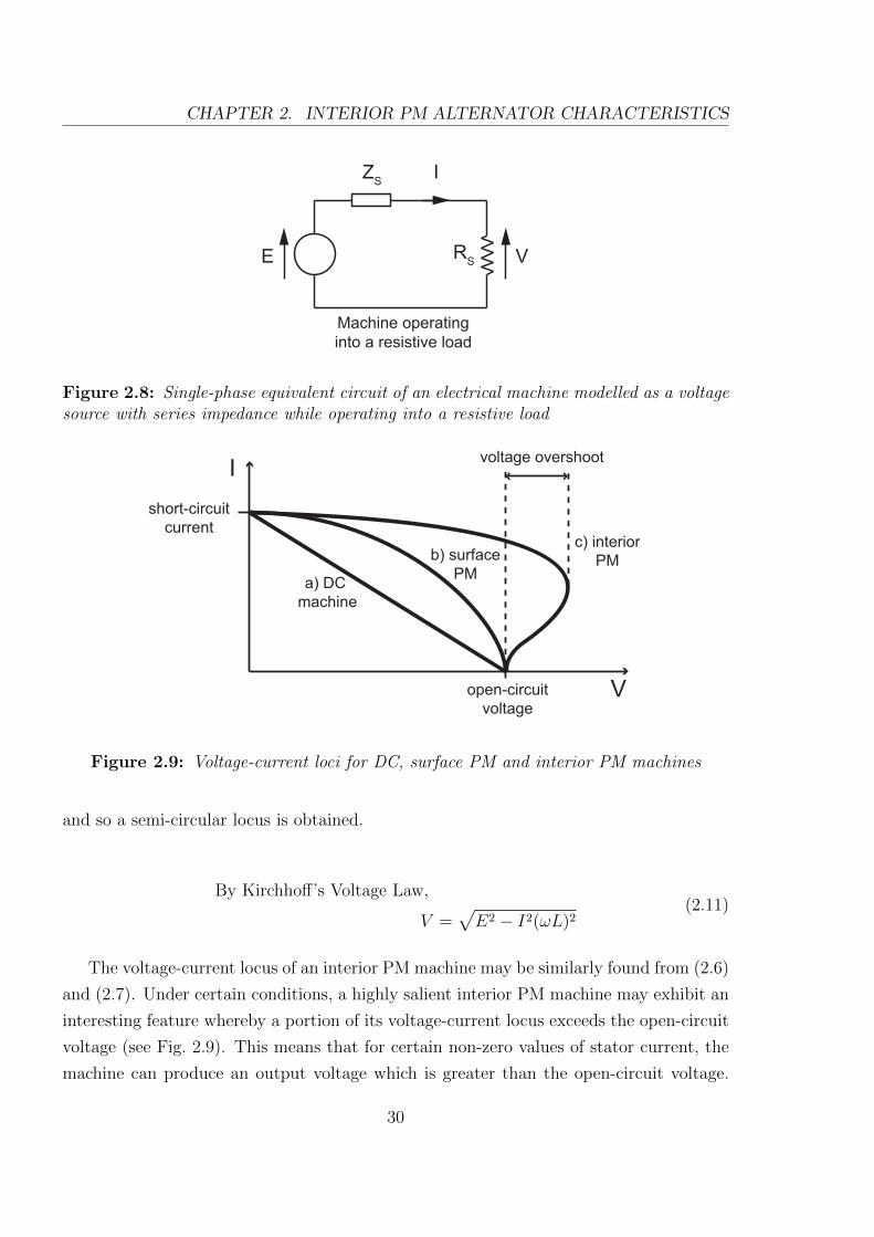
CHAPTER 2. INTERIOR PM ALTERNATOR CHARACTERISTICS
E VRS
ZS
I
Machine operating
into a resistive load
Figure 2.8: Single-phase equivalent circuit of an electrical machine modelled as a voltagesource with series impedance while operating into a resistive load
short-circuit
current
open-circuit
voltage
a) DC
machine
b) surface
PM
c) interior
PM
voltage overshootI
V
Figure 2.9: Voltage-current loci for DC, surface PM and interior PM machines
and so a semi-circular locus is obtained.
By Kirchhoff’s Voltage Law,
V =√E2 − I2(ωL)2
(2.11)
The voltage-current locus of an interior PM machine may be similarly found from (2.6)
and (2.7). Under certain conditions, a highly salient interior PM machine may exhibit an
interesting feature whereby a portion of its voltage-current locus exceeds the open-circuit
voltage (see Fig. 2.9). This means that for certain non-zero values of stator current, the
machine can produce an output voltage which is greater than the open-circuit voltage.
30

CHAPTER 2. INTERIOR PM ALTERNATOR CHARACTERISTICS
This unusual effect has been termed ’voltage overshoot’ and its magnitude is governed by
the machine’s saliency ratio.
Consider the interior PM machine operating at a certain electrical frequency ωe. The d-
q equations can be normalised using the base units defined in (2.12) to (2.14). Normalising
(2.1) and (2.2) produces (2.15) and (2.16) and from these it can be clearly seen that the
parameters affecting the shape of the voltage-current locus are the saliency ratio ξ and
the normalised stator resistance Rn, which is a function of the stator resistance Rs, the
d-axis inductance Ld and electrical frequency ωe. This normalises the VI locus to a unity
value for both open-circuit voltage and (high-speed) short-circuit current.
Vbase = ωeΨm (2.12)
Ibase = Ψm/Ld (2.13)
Rbase = Vbase/Ibase = ωeLd (2.14)
Vqn = 1 + Idn +RnIqn (2.15)
Vdn = −ξIqn +RnIdn (2.16)
where Rn =Rs
ωeLd(2.17)
2.3.1 Saliency Ratio
In the ideal case where the stator resistance Rs is neglected, the Rn terms in (2.15) and
(2.16) disappear. The only factor determining the shape of the VI locus is then the
saliency ratio, ξ of the interior PM machine. As illustrated in Fig. 2.10, a saliency ratio of
ξ = 1 would mean that the rotor is non-salient and the VI locus would be semi-circular,
exhibiting no overshoot. Voltage overshoot only occurs for interior PM machines with
ξ ≥ 2 and the amount of overshoot increases almost linearly with increasing saliency ratio
(see Fig. 2.11).
It was chosen to define voltage overshoot as the difference between the maximum
voltage Vmax on the VI locus and the machine open-circuit voltage Vo, expressed as a
percentage of Vo, i.e. overshoot% = (Vmax − Vo)/Vo × 100%.
With the Rn term eliminated, the shape of the normalised VI locus does not change
31
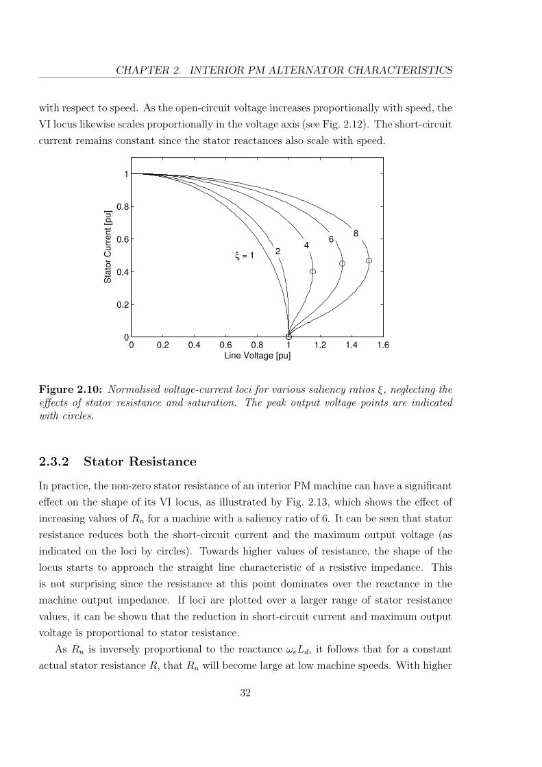
CHAPTER 2. INTERIOR PM ALTERNATOR CHARACTERISTICS
with respect to speed. As the open-circuit voltage increases proportionally with speed, the
VI locus likewise scales proportionally in the voltage axis (see Fig. 2.12). The short-circuit
current remains constant since the stator reactances also scale with speed.
0 0.2 0.4 0.6 0.8 1 1.2 1.4 1.60
0.2
0.4
0.6
0.8
1
Sta
tor
Curr
ent [p
u]
Line Voltage [pu]
8 6
42ξ = 1
Figure 2.10: Normalised voltage-current loci for various saliency ratios ξ, neglecting theeffects of stator resistance and saturation. The peak output voltage points are indicatedwith circles.
2.3.2 Stator Resistance
In practice, the non-zero stator resistance of an interior PM machine can have a significant
effect on the shape of its VI locus, as illustrated by Fig. 2.13, which shows the effect of
increasing values of Rn for a machine with a saliency ratio of 6. It can be seen that stator
resistance reduces both the short-circuit current and the maximum output voltage (as
indicated on the loci by circles). Towards higher values of resistance, the shape of the
locus starts to approach the straight line characteristic of a resistive impedance. This
is not surprising since the resistance at this point dominates over the reactance in the
machine output impedance. If loci are plotted over a larger range of stator resistance
values, it can be shown that the reduction in short-circuit current and maximum output
voltage is proportional to stator resistance.
As Rn is inversely proportional to the reactance ωeLd, it follows that for a constant
actual stator resistance R, that Rn will become large at low machine speeds. With higher
32

CHAPTER 2. INTERIOR PM ALTERNATOR CHARACTERISTICS
1 2 3 4 5 6 7 80
10
20
30
40
50
60
Saliency Ratio ξ
Vol
tage
Ove
rsho
ot [%
]
Figure 2.11: Voltage overshoot versus saliency ratio ξ, neglecting the effects of statorresistance and saturation
0 0.2 0.4 0.6 0.8 1 1.2 1.40
0.2
0.4
0.6
0.8
1
Sta
tor
Curr
ent [p
u]
Line Voltage [pu]
0.2 0.4 0.6 0.8 ωen
= 1.0 pu
Figure 2.12: Ideal voltage-current loci at various speeds ωen for saliency ratio ξ = 6,Rph = 0 pu
speeds, the effect of stator resistance becomes relatively small compared to the increasing
machine reactances. The resulting transition in the shape of the non-ideal VI locus with
33
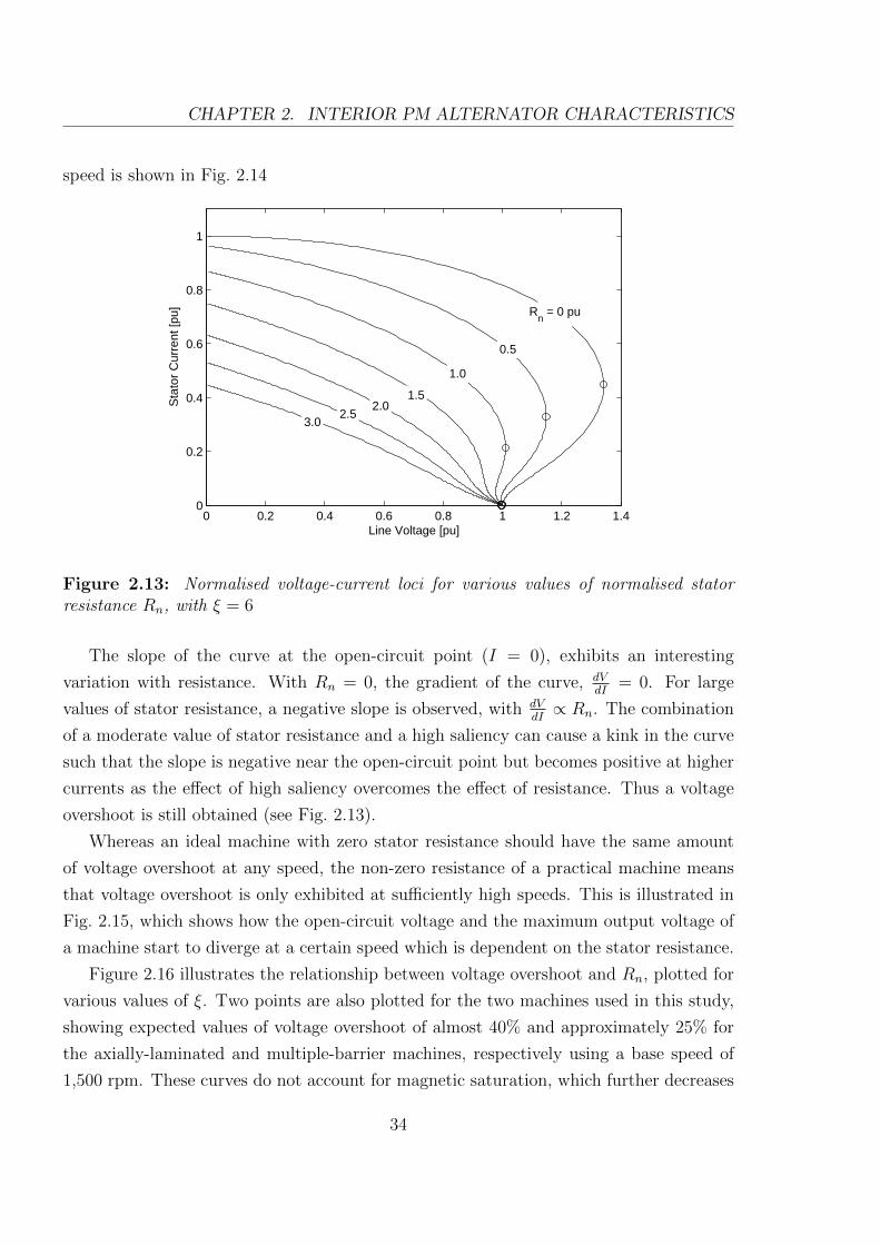
CHAPTER 2. INTERIOR PM ALTERNATOR CHARACTERISTICS
speed is shown in Fig. 2.14
0 0.2 0.4 0.6 0.8 1 1.2 1.40
0.2
0.4
0.6
0.8
1
Sta
tor
Cur
rent
[pu]
Line Voltage [pu]
Rn = 0 pu
0.5
1.0
1.52.0
2.53.0
Figure 2.13: Normalised voltage-current loci for various values of normalised statorresistance Rn, with ξ = 6
The slope of the curve at the open-circuit point (I = 0), exhibits an interesting
variation with resistance. With Rn = 0, the gradient of the curve, dVdI
= 0. For large
values of stator resistance, a negative slope is observed, with dVdI∝ Rn. The combination
of a moderate value of stator resistance and a high saliency can cause a kink in the curve
such that the slope is negative near the open-circuit point but becomes positive at higher
currents as the effect of high saliency overcomes the effect of resistance. Thus a voltage
overshoot is still obtained (see Fig. 2.13).
Whereas an ideal machine with zero stator resistance should have the same amount
of voltage overshoot at any speed, the non-zero resistance of a practical machine means
that voltage overshoot is only exhibited at sufficiently high speeds. This is illustrated in
Fig. 2.15, which shows how the open-circuit voltage and the maximum output voltage of
a machine start to diverge at a certain speed which is dependent on the stator resistance.
Figure 2.16 illustrates the relationship between voltage overshoot and Rn, plotted for
various values of ξ. Two points are also plotted for the two machines used in this study,
showing expected values of voltage overshoot of almost 40% and approximately 25% for
the axially-laminated and multiple-barrier machines, respectively using a base speed of
1,500 rpm. These curves do not account for magnetic saturation, which further decreases
34

CHAPTER 2. INTERIOR PM ALTERNATOR CHARACTERISTICS
0 0.2 0.4 0.6 0.8 1 1.2 1.40
0.2
0.4
0.6
0.8
1
Sta
tor
Curr
ent [p
u]
Line Voltage [pu]
0.2
0.40.6
0.8 ω
en = 1.0 pu
Figure 2.14: Normalised voltage-current loci at various speeds ωen, with Rn = 0.42 puat base speed
0 0.1 0.2 0.3 0.4 0.5 0.6 0.7 0.8 0.9 10
0.2
0.4
0.6
0.8
1
Machine Speed [pu]
Lin
e V
oltage [pu]
Open−Circuit VoltageMaximum Voltage
R n = 0 pu
0.2 0.40.6
0.8
Figure 2.15: Open-circuit voltage and maximum voltage vs. machine speed for variousvalues of stator resistance Rn, with ξ = 6
the voltage overshoot.
35

CHAPTER 2. INTERIOR PM ALTERNATOR CHARACTERISTICS
0 0.2 0.4 0.6 0.8 1 1.2 1.4 1.60
10
20
30
40
50
Rn
Overs
hoot [%
]
ξ = 8
7
6
5
4
3
Axially−Laminated Machine
Multiple−Barrier Machine
Figure 2.16: Voltage overshoot versus Rn for various values of saliency ratio ξ, show-ing the locations of the two test machines based on their unsaturated saliency ratio andnormalised stator resistance at 1,500 rpm
2.3.3 Magnetic Saturation
Magnetic saturation effectively reduces the saliency ratio at high stator (q-axis) currents.
As illustrated in Fig. 2.7, the reduction in the saliency is greater and occurs over a wider
current range for high values of the saturation model parameter βn. Shown in Fig. 2.17
are a range of loci for a machine with an unsaturated saliency ratio of 6 and zero stator
resistance, as βn is increased. Saturation can cause a considerable reduction in voltage
overshoot in much the same way that reducing saliency does.
The voltage overshoot that can be observed in the VI loci of highly salient interior
PM machines produces an interesting hysteretic phenomenon in their stator current vs.
speed characteristic, which is discussed in the next section.
2.4 Stator Current Hysteresis
Hysteresis in the stator current versus speed characteristic of interior PM machines during
uncontrolled generation was first discussed by Jahns [37], who modelled uncontrolled
generation from the viewpoint of motoring operation, starting with knowledge of the DC
link voltage supplied by an inverter and the machine back-emf magnitude. Jahns noted
36

CHAPTER 2. INTERIOR PM ALTERNATOR CHARACTERISTICS
0 0.2 0.4 0.6 0.8 1 1.2 1.40
0.2
0.4
0.6
0.8
1
Sta
tor
Curr
ent [p
u]
Line Voltage [pu]
βn = 8
4
2
1 0
Figure 2.17: Normalised voltage-current loci for various values of saturation parameterβn, with Rn = 0 and ξ = 6
that it was possible for an interior PM machine operating in uncontrolled generation to
continue generating current into the DC link even below the threshold speed at which
generation starts, i.e. the speed at which the rectified machine back-emf is equal to the
DC link voltage. This counter-intuitive behaviour is illustrated in a plot of stator current
vs. speed (see Fig. 2.18).
Sta
tor C
urre
nt
Machine Speed
Hysteresis Width
Figure 2.18: Typical stator current vs. speed characteristic of an interior PM machineexhibiting hysteresis
Jahns found that hysteresis was only present for saliency ratios of greater than 2 and
37

CHAPTER 2. INTERIOR PM ALTERNATOR CHARACTERISTICS
that the width of the hysteresis band was proportional to saliency and was reduced by
magnetic saturation.
In this section, VI loci will be used to explain how a hysteretic curve arises in the
stator current vs. speed characteristic of an interior PM machine. The VI locus is a simple
graphical representation of the current-voltage characteristics of the interior PM machine
with a resistive load and allows the correlation between hysteresis, voltage overshoot and
the saliency ratio to be clearly illustrated.
2.4.1 Hysteresis explained using VI Loci
Figure 2.19 shows how the voltage overshoot in the VI locus of the interior PM machine
causes hysteresis in the UCG stator current.
Consider a highly salient interior PM machine which exhibits voltage overshoot be-
ing connected via a three-phase uncontrolled rectifier to a DC voltage source and then
accelerated from standstill.
The graph on the left shows the VI locus of the machine at increasing speeds from ω1
to ω4. The graph on the right shows the stator current which the machine generates as
the speed is increased.
As the machine accelerates from standstill, it will only start to generate current into
the DC link at a certain minimum speed - this is the speed at which the open-circuit
back-emf exceeds the DC link voltage (referred to the AC side). The DC link voltage is
represented on the graph as a vertical line. The possible operating points of this system
are found where the VI locus of the machine and the DC link voltage intersect. These
points are labelled on the VI loci and likewise the corresponding stator currents produced
are labelled on the right-hand graph. At a low speed ω1, for instance, the back-emf is
lower than the DC link voltage and the diodes of the rectifier are reverse-biased. The
system operates at (A) and the output current is zero. The output voltage is the machine
open-circuit back-emf.
Generation only occurs at the higher speed of ω3, where the machine open-circuit
voltage becomes greater than the DC link voltage. The diodes become forward-biased
and current starts to flow (B). Note that the machine VI locus intersects the DC link
line at two points - at (B) where there is zero current and at (C) where there is non-
zero current. Operating point (B) is unstable, as once current starts to flow the system
immediately shifts up along the VI locus to operate at (C).
As the speed increases to ω4, the operating point moves to (D), producing slightly
38
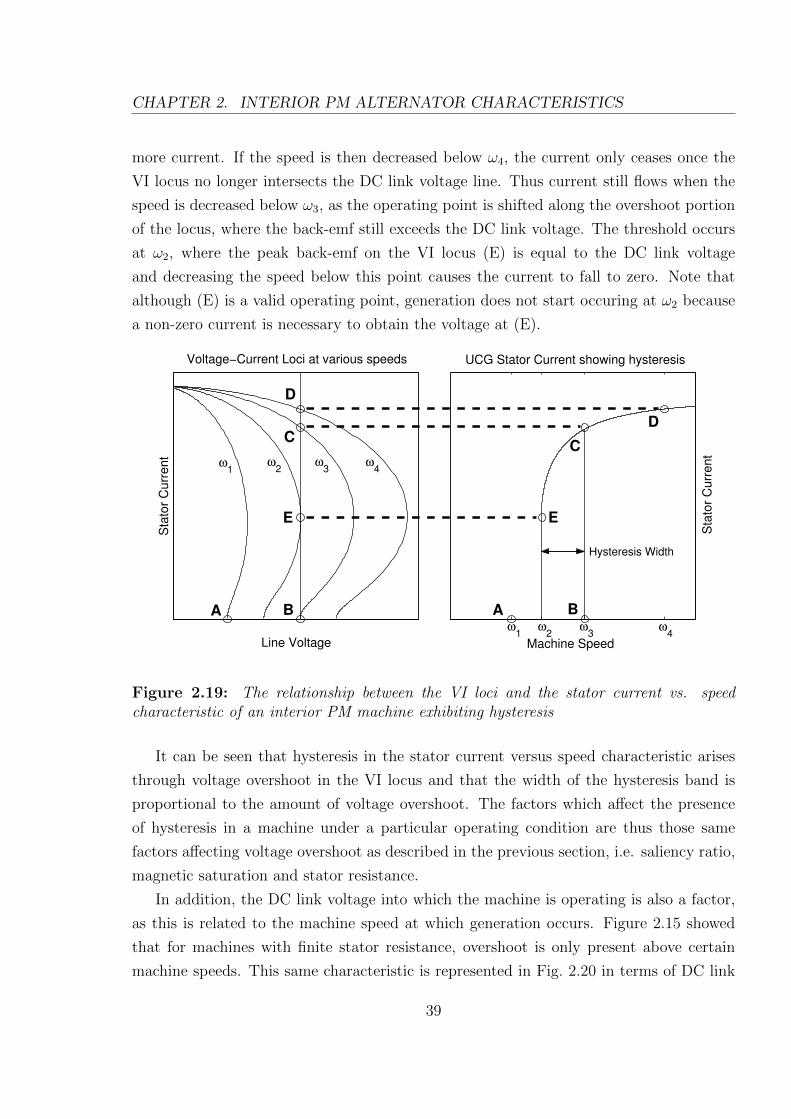
CHAPTER 2. INTERIOR PM ALTERNATOR CHARACTERISTICS
more current. If the speed is then decreased below ω4, the current only ceases once the
VI locus no longer intersects the DC link voltage line. Thus current still flows when the
speed is decreased below ω3, as the operating point is shifted along the overshoot portion
of the locus, where the back-emf still exceeds the DC link voltage. The threshold occurs
at ω2, where the peak back-emf on the VI locus (E) is equal to the DC link voltage
and decreasing the speed below this point causes the current to fall to zero. Note that
although (E) is a valid operating point, generation does not start occuring at ω2 because
a non-zero current is necessary to obtain the voltage at (E).
Sta
tor
Curr
ent
Line Voltage
Voltage−Current Loci at various speeds
Machine Speed
Sta
tor
Curr
ent
UCG Stator Current showing hysteresis
ω1 ω
2 ω
3 ω
4
A B
D
C
E
A B
C
D
E
Hysteresis Width
ω1 ω
2 ω
3 ω
4
Figure 2.19: The relationship between the VI loci and the stator current vs. speedcharacteristic of an interior PM machine exhibiting hysteresis
It can be seen that hysteresis in the stator current versus speed characteristic arises
through voltage overshoot in the VI locus and that the width of the hysteresis band is
proportional to the amount of voltage overshoot. The factors which affect the presence
of hysteresis in a machine under a particular operating condition are thus those same
factors affecting voltage overshoot as described in the previous section, i.e. saliency ratio,
magnetic saturation and stator resistance.
In addition, the DC link voltage into which the machine is operating is also a factor,
as this is related to the machine speed at which generation occurs. Figure 2.15 showed
that for machines with finite stator resistance, overshoot is only present above certain
machine speeds. This same characteristic is represented in Fig. 2.20 in terms of DC link
39

CHAPTER 2. INTERIOR PM ALTERNATOR CHARACTERISTICS
voltage, which is proportional to the speed at which conduction first occurs, where a DC
link voltage of 1 pu represents the rectified value of the machine back-emf at rated speed.
0 0.2 0.4 0.6 0.8 10
5
10
15
20
25
30
35
DC Link Voltage [pu]
Hys
tere
sis
[%]
Rn = 0 pu
0.1
0.2
0.30.4
Figure 2.20: Hysteresis versus DC link voltage for various values of Rn, with ξ = 6
2.5 Experimental Investigation
In this section, experimental results from two interior permanent magnet machines are ex-
amined in order to investigate their behaviour under UCG operation. The tests described
in the following subsections were carried out in order to achieve the following objectives:
• To test the validity of the steady-state and dynamic models used during the study
and their accuracy in predicting the output of an interior PM machine operating in
UCG;
• To experimentally demonstrate hysteresis in UCG, which had previously been pre-
dicted but not demonstrated;
• To test the validity of the approximations and assumptions made in the present as
well as earlier models of UCG operation, specifically the approximation of a rectifier
and voltage source load as a three-phase resistive load.
40
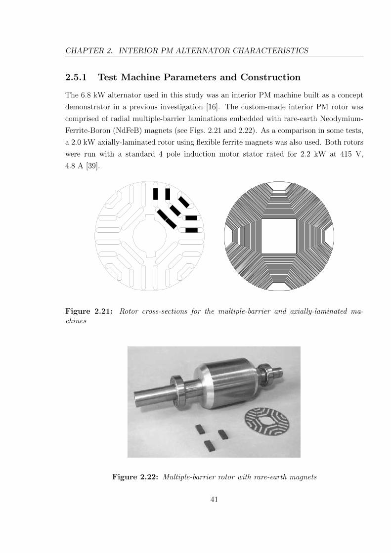
CHAPTER 2. INTERIOR PM ALTERNATOR CHARACTERISTICS
2.5.1 Test Machine Parameters and Construction
The 6.8 kW alternator used in this study was an interior PM machine built as a concept
demonstrator in a previous investigation [16]. The custom-made interior PM rotor was
comprised of radial multiple-barrier laminations embedded with rare-earth Neodymium-
Ferrite-Boron (NdFeB) magnets (see Figs. 2.21 and 2.22). As a comparison in some tests,
a 2.0 kW axially-laminated rotor using flexible ferrite magnets was also used. Both rotors
were run with a standard 4 pole induction motor stator rated for 2.2 kW at 415 V,
4.8 A [39].
Figure 2.21: Rotor cross-sections for the multiple-barrier and axially-laminated ma-chines
Figure 2.22: Multiple-barrier rotor with rare-earth magnets
41
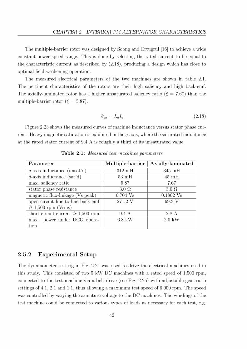
CHAPTER 2. INTERIOR PM ALTERNATOR CHARACTERISTICS
The multiple-barrier rotor was designed by Soong and Ertugrul [16] to achieve a wide
constant-power speed range. This is done by selecting the rated current to be equal to
the characteristic current as described by (2.18), producing a design which has close to
optimal field weakening operation.
The measured electrical parameters of the two machines are shown in table 2.1.
The pertinent characteristics of the rotors are their high saliency and high back-emf.
The axially-laminated rotor has a higher unsaturated saliency ratio (ξ = 7.67) than the
multiple-barrier rotor (ξ = 5.87).
Ψm = LdId (2.18)
Figure 2.23 shows the measured curves of machine inductance versus stator phase cur-
rent. Heavy magnetic saturation is exhibited in the q-axis, where the saturated inductance
at the rated stator current of 9.4 A is roughly a third of its unsaturated value.
Table 2.1: Measured test machines parameters
Parameter Multiple-barrier Axially-laminated
q-axis inductance (unsat’d) 312 mH 345 mHd-axis inductance (sat’d) 53 mH 45 mHmax. saliency ratio 5.87 7.67stator phase resistance 3.0 Ω 3.0 Ωmagnetic flux-linkage (Vs peak) 0.704 Vs 0.1802 Vsopen-circuit line-to-line back-emf@ 1,500 rpm (Vrms)
271.2 V 69.3 V
short-circuit current @ 1,500 rpm 9.4 A 2.8 Amax. power under UCG opera-tion
6.8 kW 2.0 kW
2.5.2 Experimental Setup
The dynamometer test rig in Fig. 2.24 was used to drive the electrical machines used in
this study. This consisted of two 5 kW DC machines with a rated speed of 1,500 rpm,
connected to the test machine via a belt drive (see Fig. 2.25) with adjustable gear ratio
settings of 4:1, 2:1 and 1:1, thus allowing a maximum test speed of 6,000 rpm. The speed
was controlled by varying the armature voltage to the DC machines. The windings of the
test machine could be connected to various types of loads as necessary for each test, e.g.
42

CHAPTER 2. INTERIOR PM ALTERNATOR CHARACTERISTICS
0 2 4 6 8 100
50
100
150
200
250
300
350
Phase Current (Arms)
Ind
ucta
nce
(m
H)
q−axis
d−axis
Multiple−barrier rotorAxially−laminated rotor
Figure 2.23: Measured d-axis and q-axis inductance saturation curves for the multiple-barrier and axially-laminated machines
a three-phase resistive load, a rectifier and resistive load or a rectifier and voltage source
load.
The DC voltage source load simulator depicted in Fig. 2.24 employed a series diode
to prevent damage to the laboratory power supply and a parallel resistive load in order
to absorb the power generated by the test machine. The value of this load resistance was
chosen to be able to absorb the maximum expected load current.
43

CHAPTER 2. INTERIOR PM ALTERNATOR CHARACTERISTICS
VDC
+
-
three-phase rectifier and
DC voltage source load simulator
three-phase
resistive load
rectifier and
resistive load
interior PM
machine
Vline
Iphase
IDC
IDC
Gear
Box
Variable
DC
Supply
2 × 5kW
DC
machines
VDC
+
-
Figure 2.24: Dynamometer rig test setup for testing the interior PM alternator
Figure 2.25: Variable gearbox for the dynamometer rig
44
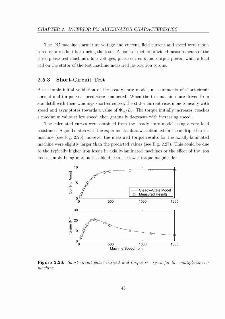
CHAPTER 2. INTERIOR PM ALTERNATOR CHARACTERISTICS
The DC machine’s armature voltage and current, field current and speed were moni-
tored on a readout box during the tests. A bank of meters provided measurements of the
three-phase test machine’s line voltages, phase currents and output power, while a load
cell on the stator of the test machine measured its reaction torque.
2.5.3 Short-Circuit Test
As a simple initial validation of the steady-state model, measurements of short-circuit
current and torque vs. speed were conducted. When the test machines are driven from
standstill with their windings short-circuited, the stator current rises monotonically with
speed and asymptotes towards a value of Ψm/Ld. The torque initially increases, reaches
a maximum value at low speed, then gradually decreases with increasing speed.
The calculated curves were obtained from the steady-state model using a zero load
resistance. A good match with the experimental data was obtained for the multiple-barrier
machine (see Fig. 2.26), however the measured torque results for the axially-laminated
machine were slightly larger than the predicted values (see Fig. 2.27). This could be due
to the typically higher iron losses in axially-laminated machines or the effect of the iron
losses simply being more noticeable due to the lower torque magnitude.
0 500 1000 15000
5
10
Curr
ent [A
rms]
0 500 1000 15000
10
20
30
Machine Speed [rpm]
Torq
ue [N
m]
Steady−State ModelMeasured Results
Figure 2.26: Short-circuit phase current and torque vs. speed for the multiple-barriermachine
45

CHAPTER 2. INTERIOR PM ALTERNATOR CHARACTERISTICS
0 500 1000 15000
1
2
3
Sta
tor
Curr
ent [A
rms]
Steady−State ModelMeasured Results
0 500 1000 15000
1
2
3
Machine Speed [rpm]
Torq
ue [N
m]
Figure 2.27: Short-circuit phase current and torque vs. speed for the axially-laminatedmachine
46

CHAPTER 2. INTERIOR PM ALTERNATOR CHARACTERISTICS
2.5.4 Three-Phase Resistive Load Test
A three-phase resistive load is the load upon which the steady-state model of UCG is
directly based and also the simplest load to analyse. Hence, the results are most likely to
match the model predictions.
The test machines were run at 1,500 rpm into a three-phase resistive load and the stator
currents and line voltages were measured for various values of load resistance in order to
obtain VI loci. Figure 2.28 shows the measured and predicted results for the multiple-
barrier machine. The ideal model prediction shown does not take into account stator
resistance or magnetic saturation and exhibits approximately 30% voltage overshoot. The
effect of stator resistance alone reduces the predicted overshoot from 30% to 22%, whereas
the effect of magnetic saturation alone reduces the predicted overshoot from 30% to
14%, hence playing a larger part in reducing the overshoot than stator resistance for this
machine at this speed. The combination of these two effects act to reduce the predicted
overshoot from 30% to a mere 7%.
For the axially-laminated machine, the maximum q-axis current obtainable at 1,500 rpm
regardless of the value of load resistance is approximately 0.5 A. Referring to Fig. 2.23,
this current is still in the unsaturated region of Lq so the machine does not experience
magnetic saturation, which can therefore be neglected. Although the decrease in current
due to stator resistance is much more noticeable than in the multiple-barrier machine,
the reduction of the predicted overshoot from 56% of the open-circuit voltage to 50% is
less dramatic (see Fig. 2.29).
The measured VI loci from both interior PM machines are closely matched by the
steady-state model predictions, indicating that the model is reasonably accurate.
47
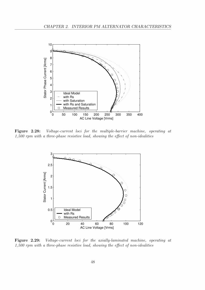
CHAPTER 2. INTERIOR PM ALTERNATOR CHARACTERISTICS
0 50 100 150 200 250 300 350 4000
1
2
3
4
5
6
7
8
9
10S
tato
r P
hase C
urr
ent [A
rms]
AC Line Voltage [Vrms]
Ideal Modelwith Rswith Saturationwith Rs and SaturationMeasured Results
Figure 2.28: Voltage-current loci for the multiple-barrier machine, operating at1,500 rpm with a three-phase resistive load, showing the effect of non-idealities
0 20 40 60 80 100 1200
0.5
1
1.5
2
2.5
3
Sta
tor
Curr
ent [A
rms]
AC Line Voltage [Vrms]
Ideal Modelwith RsMeasured Results
Figure 2.29: Voltage-current loci for the axially-laminated machine, operating at1,500 rpm with a three-phase resistive load, showing the effect of non-idealities
48

CHAPTER 2. INTERIOR PM ALTERNATOR CHARACTERISTICS
2.5.5 Generation into a Rectifier and Resistive Load
In this test, both machines were run at speeds of 1,800, 3,000 and 6,000 rpm into a
three-phase rectifier and resistive load (see Fig. 2.5b) and current, voltage and power
measurements were taken. AC measurements were taken at the machine windings and
DC measurements were taken across the resistive load. These measurements allow an
observation of how the AC VI loci translate to DC output, which reflects on the validity
of simplifying a rectifier and resistive load as a three-phase resistive load in the steady-
state model of UCG.
The theoretical loci at the output of the rectifier were obtained by scaling the the AC
predictions by the theoretical ratio of the rectified DC to rms AC values. These ratios
are 1.355 for current and 1.283 for voltage.
0 100 200 300 400 5000
2
4
6
8
10
Sta
tor
Curr
ent [A
rms]
AC Line Voltage [Vrms]
AC (Multiple−Barrier)
1800rpm
3000rpm
6000rpm
0 100 200 300 400 5000
2
4
6
AC Line Voltage [Vrms]
AC
Outp
ut P
ow
er
[kW
]
1800rpm
3000rpm
6000rpm
Figure 2.30: AC VI and VP loci for the multiple-barrier machine at various speeds,showing calculated curves (lines) and measured results (circles)
Figure 2.30 shows the measured voltage-current and voltage-power loci together with
the steady-state model predictions for the multiple-barrier machine. The AC results match
well with the predictions although the current obtained is slightly smaller than predicted.
There is however a significant discrepancy in the corresponding DC output curves (see
Fig. 2.31) at lower values of current corresponding to the voltage overshoot region. The
measured overshoot for the multiple-barrier machine at 1500 rpm is thus reduced tenfold,
from 10% in the AC curves to about 1% in the DC curves.
49

CHAPTER 2. INTERIOR PM ALTERNATOR CHARACTERISTICS
0 100 200 300 400 500 6000
5
10
15
DC Output Voltage [V]
DC
Outp
ut C
urr
ent [A
]
DC (Multiple−Barrier)
1800rpm
3000rpm
6000rpm
0 100 200 300 400 500 6000
2
4
6
DC Output Voltage [V]
DC
Outp
ut P
ow
er
[kW
]
1800rpm
3000rpm
6000rpm
Figure 2.31: DC VI and VP loci for the multiple-barrier machine at various speeds,showing calculated curves (lines) and measured results (circles)
The multiple-barrier machine results show that at higher speeds the stator current
becomes nearly constant with respect to line voltage and the output power is almost
linearly related to output voltage. They also show that at rated line voltage (415 V) the
machine is capable of producing around 6 kW of output power at 6,000 rpm.
The results for the axially-laminated machine (see Figs. 2.32 and 2.33) exhibit the
same trends as those found with the multiple-barrier machine. The measured AC curves
show a good correspondence with the steady-state model predictions, whereas once again
significant discrepancy is noted in the DC curves, which show a lower than predicted
maximum voltage on the overshoot portion of the loci.
One feature which occurs in both the multiple-barrier machine and the axially-laminated
machine is the unusual shape of the measured DC curve towards lower currents - the open-
circuit voltage appears higher than predicted and as the current increases from zero, the
voltage at first decreases before starting to rise as the operating point enters the voltage
overshoot region.
The decreased maximum overshoot voltage in the axially-laminated machine means
that it will stop generating at a higher speed than predicted, causing a reduction of
overshoot in the DC loci from 39% to 23%, which corresponds to a reduction factor of 1.7
which is consistent for both the 750 rpm and 1,500 rpm curves. As this significant voltage
50

CHAPTER 2. INTERIOR PM ALTERNATOR CHARACTERISTICS
overshoot reduction in both machines was not observed in the AC side loci, it may be due
to the discontinuous current waveforms present in this region.
0 20 40 60 80 1000
1
2
3
Sta
tor
Cu
rre
nt
[Arm
s]
AC Line Voltage [Vrms]
AC (Ax−Lam)
750rpm 1500rpm
0 20 40 60 80 1000
0.1
0.2
0.3
AC Line Voltage [Vrms]
AC
Ou
tpu
t P
ow
er
[kW
]
750rpm
1500rpm
Figure 2.32: AC VI and VP loci for the axially-laminated machine at various speeds,showing calculated curves (lines) and measured results (circles)
51

CHAPTER 2. INTERIOR PM ALTERNATOR CHARACTERISTICS
0 20 40 60 80 100 1200
1
2
3
4
DC Output Voltage [V]
DC
Ou
tpu
t C
urr
en
t [A
]
DC (Ax−Lam)
750rpm 1500rpm
0 20 40 60 80 100 1200
0.1
0.2
0.3
DC Output Voltage [V]
DC
Ou
tpu
t P
ow
er
[kW
]
750rpm
1500rpm
Figure 2.33: DC VI and VP loci for the axially-laminated machine at various speeds,showing calculated curves (lines) and measured results (circles)
52
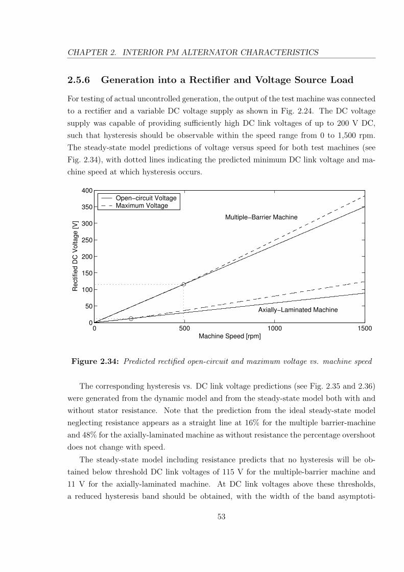
CHAPTER 2. INTERIOR PM ALTERNATOR CHARACTERISTICS
2.5.6 Generation into a Rectifier and Voltage Source Load
For testing of actual uncontrolled generation, the output of the test machine was connected
to a rectifier and a variable DC voltage supply as shown in Fig. 2.24. The DC voltage
supply was capable of providing sufficiently high DC link voltages of up to 200 V DC,
such that hysteresis should be observable within the speed range from 0 to 1,500 rpm.
The steady-state model predictions of voltage versus speed for both test machines (see
Fig. 2.34), with dotted lines indicating the predicted minimum DC link voltage and ma-
chine speed at which hysteresis occurs.
0 500 1000 15000
50
100
150
200
250
300
350
400
Rectified D
C V
oltage [V
]
Machine Speed [rpm]
Multiple−Barrier Machine
Axially−Laminated Machine
Open−circuit VoltageMaximum Voltage
Figure 2.34: Predicted rectified open-circuit and maximum voltage vs. machine speed
The corresponding hysteresis vs. DC link voltage predictions (see Fig. 2.35 and 2.36)
were generated from the dynamic model and from the steady-state model both with and
without stator resistance. Note that the prediction from the ideal steady-state model
neglecting resistance appears as a straight line at 16% for the multiple barrier-machine
and 48% for the axially-laminated machine as without resistance the percentage overshoot
does not change with speed.
The steady-state model including resistance predicts that no hysteresis will be ob-
tained below threshold DC link voltages of 115 V for the multiple-barrier machine and
11 V for the axially-laminated machine. At DC link voltages above these thresholds,
a reduced hysteresis band should be obtained, with the width of the band asymptoti-
53

CHAPTER 2. INTERIOR PM ALTERNATOR CHARACTERISTICS
cally approaching the ideal hysteresis width value as the DC link voltage increases. The
dynamic model prediction (which includes resistance) lies roughly mid-way between the
steady-state model predictions with and without resistance.
The actual hysteresis measured for the axially-laminated machine is significantly smaller
than that predicted by the steady-state model. If the overshoot reduction factor of 1.7
observed earlier in the measured VI loci is incorporated into the steady-state prediction,
it can be seen that the measured points are more consistent with the resultant adjusted
curve. Experimental points were only taken up to a DC link voltage of 80 V, due to the
axially-laminated machine’s maximum test speed of 1,500 rpm.
Figure 2.36 shows that the hysteresis predictions of the steady-state model with re-
sistance and the dynamic model predictions were comparable for the multiple-barrier
machine. No hysteresis was observed experimentally with the multiple-barrier machine,
even with measurements being taken up to 250 V. Taking into account the tenfold de-
crease previously observed in the measured voltage overshoot between the AC and DC
curves, the expected hysteresis is only approximately 1%. This corresponds to a speed
range of 15 rpm at this test speed, which may have been too small to detect with the
experimental setup used.
0 50 100 1500
10
20
30
40
50
60
% H
yste
resis
DC Link Voltage [V]
Steady−state Model (no Rs)Steady−state Model (with Rs)Adjusted Steady−state ModelDynamic ModelMeasured Results
Figure 2.35: Model predictions and measured hysteresis band as a function of the DClink voltage for the axially-laminated machine
54

CHAPTER 2. INTERIOR PM ALTERNATOR CHARACTERISTICS
0 50 100 150 200 250 3000
2
4
6
8
10
12
14
16
18
20
% H
yste
resis
DC Link Voltage [V]
Steady−state Model (no Rs)Steady−state Model (with Rs)Adjusted Steady−state ModelDynamic ModelMeasured Results
Figure 2.36: Model predictions and measured hysteresis band as a function of the DClink voltage for the multiple-barrier machine
Figures 2.37 and 2.38 show examples of measured stator current versus speed charac-
teristics from which the hysteresis data points in Figures 2.36 and 2.35 were obtained, for
the multiple-barrier rotor and the axially-laminated rotor respectively.
The stator current was recorded as the machine speed was increased slowly from
standstill up to 1,500 rpm and then decreased until generation ceased. Figure 2.38 shows
the axially-laminated machine operating into a DC link voltage of 40 V. The upper half of
the figure shows calculated VI loci for the machine at increasing speeds, with the DC link
voltage (referred to the machine AC side) indicated as a solid vertical line. The lower half
shows a plot of measured stator current versus speed, overlaid with calculated curves from
the dynamic model and from the steady-state models both with and without resistance.
The axially-laminated machine exhibited a measured hysteresis band of approximately
15%, which is significantly smaller than the steady-state prediction of 25%, but close to
the dynamic model prediction of 18%.
Figure 2.37 shows the multiple-barrier machine operating into a DC link voltage of
110 V, where no hysteresis was observed. The reason for this is evident in the VI loci
which indicate that generation begins at around 480 rpm, where the open-circuit back-emf
crosses the DC link voltage line. At this speed there is almost no overshoot in the VI
55

CHAPTER 2. INTERIOR PM ALTERNATOR CHARACTERISTICS
locus and hence no observable hysteresis.
While all three models could accurately predict the speed at which generation starts,
it can be seen that the steady-state model prediction incorporating resistance generally
shows the best match with the measured results, particularly at higher speeds. In com-
parison, the dynamic model tends to slightly overestimate the current throughout the
curve but provides a more accurate prediction of the speeds at which generation begins
and ends. This can be more clearly seen in Fig. 2.32, which shows an enlarged view of
the speed range over which hysteresis occurs. The steady-state model neglecting resis-
tance overestimates both the stator current magnitude and the hysteresis considerably, as
shown in the case of the 110 V DC link voltage where it incorrectly predicts the presence
of hysteresis where there is none (see Fig. 2.36).
0 50 100 150 200 250 3000
2
4
6
8
10
100 300 500700 900 1100 1300 1500
Sta
tor
Curr
ent [A
rms]
Stator Line Voltage [Vrms]
0 500 1000 15000
2
4
6
8
10
Sta
tor
Curr
ent [A
rms]
Machine Speed [rpm]
Steady−state model (no Rs)Steady−state model (with Rs)Dynamic modelMeasured Results
DC Link Voltage
Figure 2.37: Calculated and measured UCG stator current characteristic with speed forthe multiple-barrier machine operating into a 110V DC voltage source
Several oscilloscope screenshots of the stator current and voltage waveforms are shown
in Fig. 2.40, taken from the multiple-barrier machine operating into a rectifier and voltage
source load of 110 V. At rated speed (1,500 rpm) where the back-emf voltage is much
higher than the DC link voltage, the stator current is sinusoidal while the stator line
56

CHAPTER 2. INTERIOR PM ALTERNATOR CHARACTERISTICS
0 20 40 60 80 1000
1
2
3
100
300500 700 900 1100 1300
1500S
tato
r C
urr
en
t [A
rms]
Stator Line Voltage [Vrms]
0 500 1000 15000
1
2
3
Sta
tor
Cu
rre
nt
[Arm
s]
Machine Speed [rpm]
Steady−state model (no Rs)Steady−state model (with Rs)Dynamic modelMeasured Results
DC Link Voltage
Figure 2.38: Calculated and measured UCG stator current characteristic with speed forthe axially-laminated machine operating into a 40V DC voltage source
voltage resembles the normal six-step waveform from an inverter, ranging from 110 V to
-110 V.
As the speed is reduced to 504 rpm, the machine back-emf becomes comparable to
the DC link voltage, the current waveform becomes non-sinusoidal and the line voltage
waveform transitions start to become smoother (note the change in the scaling of the
current axis). This trend continues down to a low speed close to the generation threshold
(482 rpm), where the current starts to resemble a six-step waveform and the voltage is
more sinusoidal.
The waveform shapes are accurately predicted by the dynamic model, although there
is some discrepancy in the magnitude of the current at 504 rpm.
2.6 Summary of Findings
The work in this chapter has produced findings which represent new contributions in the
area of interior PM machines, which can be used as a high power alternator in vehicles:
57
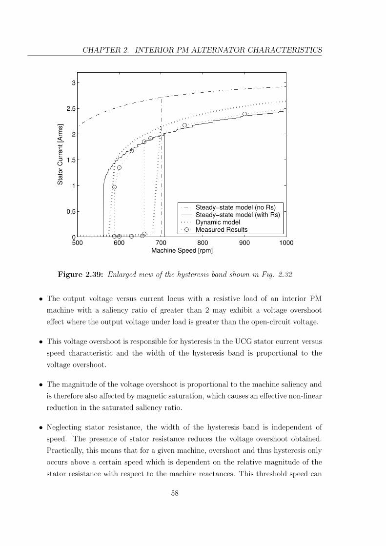
CHAPTER 2. INTERIOR PM ALTERNATOR CHARACTERISTICS
500 600 700 800 900 10000
0.5
1
1.5
2
2.5
3
Sta
tor
Cu
rre
nt
[Arm
s]
Machine Speed [rpm]
Steady−state model (no Rs)Steady−state model (with Rs)Dynamic modelMeasured Results
Figure 2.39: Enlarged view of the hysteresis band shown in Fig. 2.32
• The output voltage versus current locus with a resistive load of an interior PM
machine with a saliency ratio of greater than 2 may exhibit a voltage overshoot
effect where the output voltage under load is greater than the open-circuit voltage.
• This voltage overshoot is responsible for hysteresis in the UCG stator current versus
speed characteristic and the width of the hysteresis band is proportional to the
voltage overshoot.
• The magnitude of the voltage overshoot is proportional to the machine saliency and
is therefore also affected by magnetic saturation, which causes an effective non-linear
reduction in the saturated saliency ratio.
• Neglecting stator resistance, the width of the hysteresis band is independent of
speed. The presence of stator resistance reduces the voltage overshoot obtained.
Practically, this means that for a given machine, overshoot and thus hysteresis only
occurs above a certain speed which is dependent on the relative magnitude of the
stator resistance with respect to the machine reactances. This threshold speed can
58
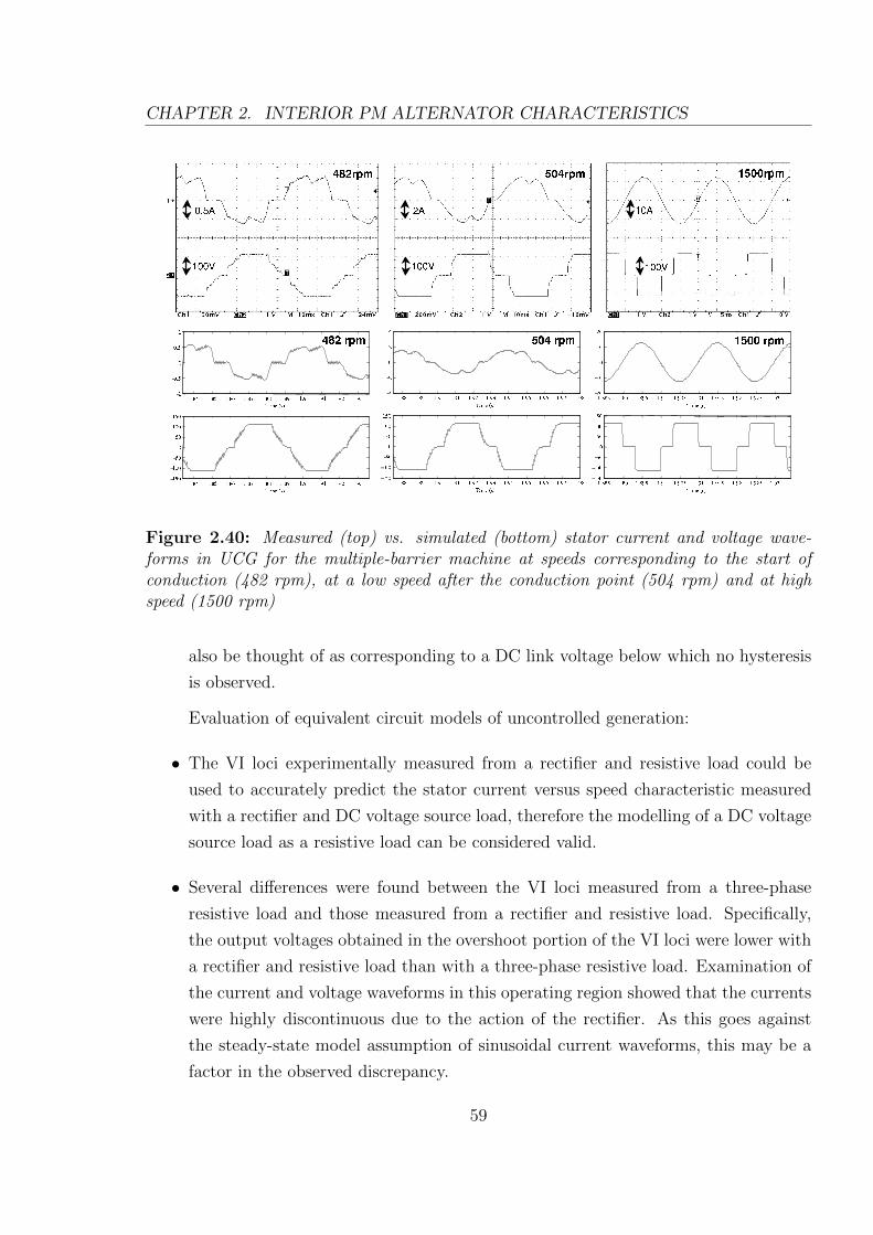
CHAPTER 2. INTERIOR PM ALTERNATOR CHARACTERISTICS
Figure 2.40: Measured (top) vs. simulated (bottom) stator current and voltage wave-forms in UCG for the multiple-barrier machine at speeds corresponding to the start ofconduction (482 rpm), at a low speed after the conduction point (504 rpm) and at highspeed (1500 rpm)
also be thought of as corresponding to a DC link voltage below which no hysteresis
is observed.
Evaluation of equivalent circuit models of uncontrolled generation:
• The VI loci experimentally measured from a rectifier and resistive load could be
used to accurately predict the stator current versus speed characteristic measured
with a rectifier and DC voltage source load, therefore the modelling of a DC voltage
source load as a resistive load can be considered valid.
• Several differences were found between the VI loci measured from a three-phase
resistive load and those measured from a rectifier and resistive load. Specifically,
the output voltages obtained in the overshoot portion of the VI loci were lower with
a rectifier and resistive load than with a three-phase resistive load. Examination of
the current and voltage waveforms in this operating region showed that the currents
were highly discontinuous due to the action of the rectifier. As this goes against
the steady-state model assumption of sinusoidal current waveforms, this may be a
factor in the observed discrepancy.
59

CHAPTER 2. INTERIOR PM ALTERNATOR CHARACTERISTICS
• The simulation results were experimentally validated using two high-saliency interior
PM machines. An extensive comparison of the simulation and test results were
performed including short-circuit, three-phase resistive load, rectifier and resistive
load, and rectifier and voltage source load.
• The predicted stator current hysteresis was demonstrated in one of the test ma-
chines.
60
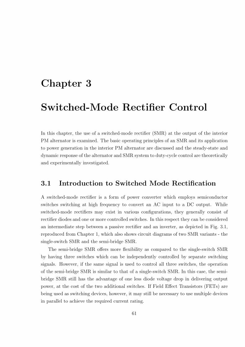
Chapter 3
Switched-Mode Rectifier Control
In this chapter, the use of a switched-mode rectifier (SMR) at the output of the interior
PM alternator is examined. The basic operating principles of an SMR and its application
to power generation in the interior PM alternator are discussed and the steady-state and
dynamic response of the alternator and SMR system to duty-cycle control are theoretically
and experimentally investigated.
3.1 Introduction to Switched Mode Rectification
A switched-mode rectifier is a form of power converter which employs semiconductor
switches switching at high frequency to convert an AC input to a DC output. While
switched-mode rectifiers may exist in various configurations, they generally consist of
rectifier diodes and one or more controlled switches. In this respect they can be considered
an intermediate step between a passive rectifier and an inverter, as depicted in Fig. 3.1,
reproduced from Chapter 1, which also shows circuit diagrams of two SMR variants - the
single-switch SMR and the semi-bridge SMR.
The semi-bridge SMR offers more flexibility as compared to the single-switch SMR
by having three switches which can be independently controlled by separate switching
signals. However, if the same signal is used to control all three switches, the operation
of the semi-bridge SMR is similar to that of a single-switch SMR. In this case, the semi-
bridge SMR still has the advantage of one less diode voltage drop in delivering output
power, at the cost of the two additional switches. If Field Effect Transistors (FETs) are
being used as switching devices, however, it may still be necessary to use multiple devices
in parallel to achieve the required current rating.
61

CHAPTER 3. SWITCHED-MODE RECTIFIER CONTROL
VDC
+
-
VDC
+
-
a) b)
VDC
+
-
VDC
+
-
c) d)
Figure 3.1: Three-phase AC machines operating into a voltage source load via: a) abridge rectifier, b) an inverter, c) a semi-bridge SMR, and d) a single-switch SMR
The use of a switched-mode rectifier at the output of the interior PM alternator in
this study was investigated as a means to accomplish two objectives - to maximise output
power at any alternator speed when operating into a constant voltage source and to
perform output voltage regulation, particularly to reduce output voltage transients under
load dump conditions.
Both SMR configurations were used in this study - the semi-bridge rectifier is examined
in Chapter 4 for the improvement of low speed output power, but for the purpose of
investigating the basic characteristics of switched-mode rectifier operation, a single-switch
SMR is considered. Similar work with a single-switch SMR was previously undertaken
by Perreault, who investigated the load-matching performance of an SMR to maximise
power transfer from a Lundell alternator [9]. This study demonstrated the ability of the
SMR to improve alternator power output at high speeds, as well as to suppress voltage
transients.
62

CHAPTER 3. SWITCHED-MODE RECTIFIER CONTROL
VDC
+
-
V dEFF
+
-
Figure 3.2: Interior PM alternator operating with an SMR into a DC voltage sourceload
3.2 SMR Operation
Figure 3.2 shows the interior PM alternator operating into a DC voltage source load with
a single-switch SMR. A pulse width modulated (PWM) control signal is used to turn the
SMR switch on and off at high frequency. With the switch turned on, the alternator
windings are short-circuited and current increases in the machine windings. When the
switch is off, the current flows through the diode into the DC link. With a sufficiently
large alternator winding inductance, the machine sees only the time-averaged effect of the
switching. This serves two purposes, depending on the operating speed of the alternator.
At low speeds where the rectified alternator back-emf is less than the DC link voltage,
no generation will occur if the switch is off. However, during SMR switching, the buildup
of current in the machine winding inductances while the switch is closed allows a portion
of current to pass through to the DC link after the switch opens, even against the higher
voltage. In this manner, the SMR acts similarly to a boost rectifier, effectively increasing
the machine output voltage but reducing its effective output current. This effect can
also be viewed as a reduction in the effective DC link voltage seen by the alternator (see
Fig. 3.3). Thus, if a voltage VDC is present at the DC link, applying a PWM control
signal of duty-cycle d will lower the effective DC link voltage VEFF seen by the alternator,
according to (3.1).
VEFF = (1− d)VDC (3.1)
Note that although the effective DC link voltage decreases with increasing SMR duty-
cycle, so does the proportion of current actually delivered to the DC link as shown in
63
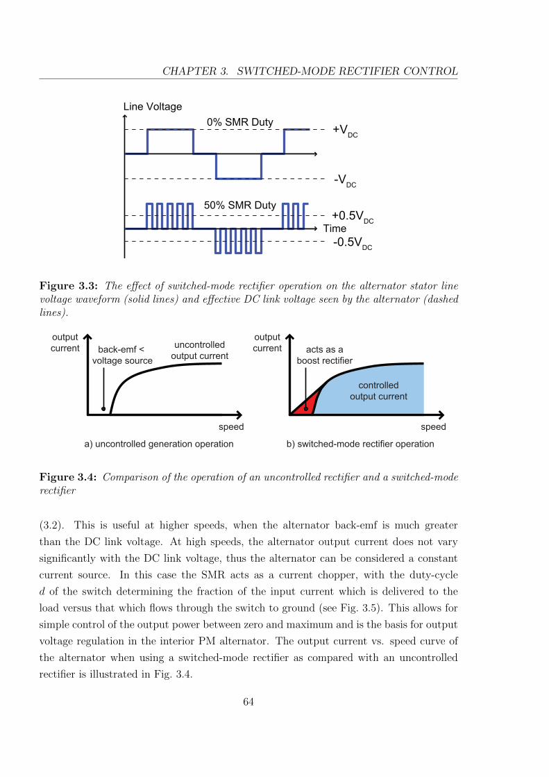
CHAPTER 3. SWITCHED-MODE RECTIFIER CONTROL
0% SMR Duty
Line Voltage
Time
+VDC
+0.5VDC
-0.5VDC
-VDC
50% SMR Duty
Figure 3.3: The effect of switched-mode rectifier operation on the alternator stator linevoltage waveform (solid lines) and effective DC link voltage seen by the alternator (dashedlines).
speed
controlled
output current
output
current acts as a
boost rectifier
speed
uncontrolled
output current
a) uncontrolled generation operation b) switched-mode rectifier operation
output
current back-emf <
voltage source
Figure 3.4: Comparison of the operation of an uncontrolled rectifier and a switched-moderectifier
(3.2). This is useful at higher speeds, when the alternator back-emf is much greater
than the DC link voltage. At high speeds, the alternator output current does not vary
significantly with the DC link voltage, thus the alternator can be considered a constant
current source. In this case the SMR acts as a current chopper, with the duty-cycle
d of the switch determining the fraction of the input current which is delivered to the
load versus that which flows through the switch to ground (see Fig. 3.5). This allows for
simple control of the output power between zero and maximum and is the basis for output
voltage regulation in the interior PM alternator. The output current vs. speed curve of
the alternator when using a switched-mode rectifier as compared with an uncontrolled
rectifier is illustrated in Fig. 3.4.
64

CHAPTER 3. SWITCHED-MODE RECTIFIER CONTROL
The constant duty-cycle control, which effectively produces a six-step voltage waveform
at the motor terminals, causes distortion of the current waveform, particularly at lower
speeds.
IOUT = (1− d)IIN (3.2)
Alternator
ISW
= IIN
(d)
IIN
IOUT
= IIN
(1-d)
VDC
+
-
0 1
IIN
IOUT
ISW
duty-cycle (d)
Figure 3.5: Duty-cycle control of alternator output current with the alternator operatingas a constant current source at high speeds
3.3 SMR Modelling
The effects of SMR switching using (3.1) and (3.2) can be illustrated in the scaling of the
calculated interior PM machine VI loci as duty-cycle is varied. Figure 3.6 shows VI loci
calculated using the steady-state model developed in the previous chapter after modifica-
tions to incorporate the effects of SMR switching. The ability to lower the effective DC
link voltage allows the alternator to generate current at speeds below the normal genera-
tion threshold (see Fig. 3.4) and so the SMR duty-cycle can be adjusted to obtain useful
output power down to very low speeds, as indicated by the line of maximum current in
Fig. 3.7.
The output current of the SMR is dependent on the switching duty-cycle according to
the relationship in (3.2), while the output power of the alternator is dependent on both
the operating speed and the effective DC link voltage seen by the machine, as discussed in
the previous chapter. If the actual DC link voltage is assumed to be the constant 200 V as
specified for the SMR module, varying the parameters of duty-cycle and alternator speed
65

CHAPTER 3. SWITCHED-MODE RECTIFIER CONTROL
0 0.5 1 1.5 2 2.5 3 3.5 4 4.5 50
0.2
0.4
0.6
0.8
1
Sta
tor
Cu
rre
nt
[pu
]
Line Voltage [pu]
0% duty
25%
50%
75%
100%
Figure 3.6: Calculated scaling effect of duty-cycle on interior PM alternator VI locus
0 0.2 0.4 0.6 0.8 10
0.2
0.4
0.6
0.8
1
Alternator Speed [pu]
Inp
ut
Cu
rre
nt
[pu
]
0% duty25%
50%
75%
100%
0 0.2 0.4 0.6 0.8 10
0.2
0.4
0.6
0.8
1
Alternator Speed [pu]
Ou
tpu
t C
urr
en
t [p
u]
0%
25%
50%
75%
100% duty
maximum current
Figure 3.7: Calculated scaling effect of duty-cycle on alternator input and output current
produces a contour plot of DC output current as shown in Fig. 3.8. In the lower-left region
of the contour plot, no output current is produced as the back-emf of the machine cannot
overcome the DC link voltage. The slope of the contour illustrates the characteristic of
the SMR whereby increasing the duty-cycle at operating speeds below 3,000 rpm may
allow more current to be obtained but at the same time imposes an upper limit to the
maximum obtainable output current. It can be seen that the traces in the right-hand
66

CHAPTER 3. SWITCHED-MODE RECTIFIER CONTROL
plot of Fig. 3.7 correspond to horizontal cross-sections of Fig. 3.8 at different duty-cycles.
The line of maximum output current for a given speed is also similarly indicated on the
contour plot.
A contour plot of efficiency can also be plotted (see Fig. 3.9). The efficiency is generally
greater at lower speeds and at lower duty-cycles - the iron losses increase rapidly with
speed and higher duty-cycles mean that a higher proportion of current flows through the
SMR switch rather than to the load and hence the output power is lower.
1000 2000 3000 4000 5000 60000
10
20
30
40
50
60
70
80
90
100
Alternator Speed [rpm]
Duty
Cycle
[%
]
30
25
20
15
10
5
maxim
um
curre
nt
Figure 3.8: Contour plot of calculated DC output current vs. duty-cycle and alternatorspeed for a 200 V DC link voltage.
67
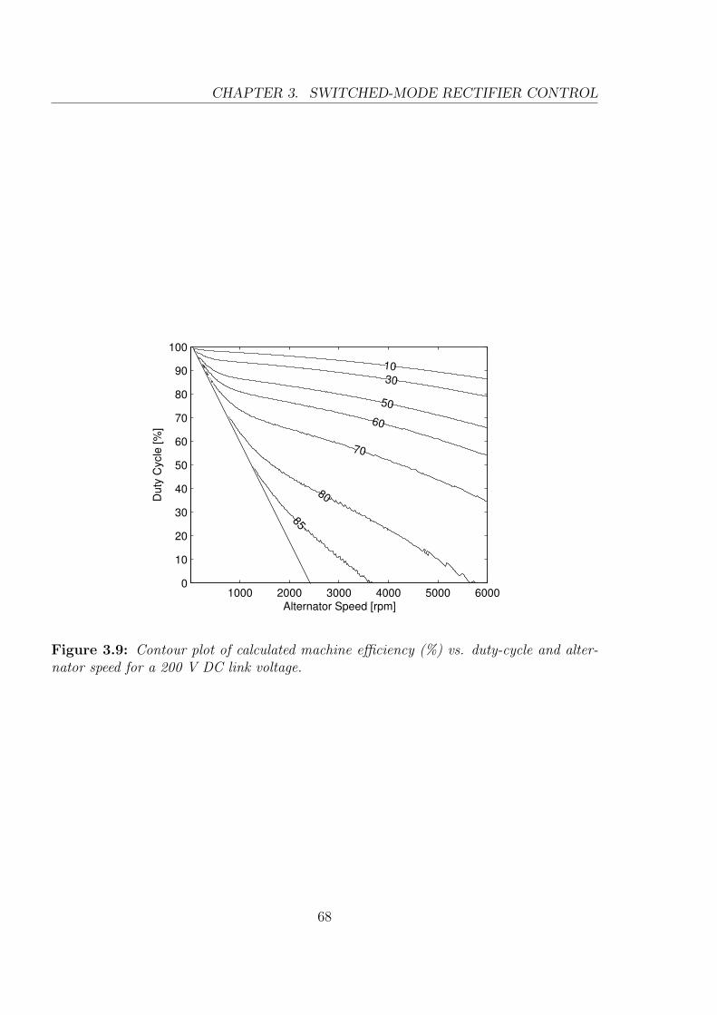
CHAPTER 3. SWITCHED-MODE RECTIFIER CONTROL
1000 2000 3000 4000 5000 60000
10
20
30
40
50
60
70
80
90
100
Alternator Speed [rpm]
Duty
Cycle
[%
]
85
80
70
60
50
30
10
Figure 3.9: Contour plot of calculated machine efficiency (%) vs. duty-cycle and alter-nator speed for a 200 V DC link voltage.
68

CHAPTER 3. SWITCHED-MODE RECTIFIER CONTROL
3.4 Experimental Setup
The switched-mode rectifier power electronics unit used was based on an existing 200 V,
50 A, three-phase inverter (see Fig. 3.10). So as to match the inverter voltage rating,
the interior PM alternator was fitted with a 135 V stator instead of the 415 V stator
used in Chapter 2. This stator was wound with the same total amount of copper as the
415 V stator but using a third of the original number of turns and triple the original
wire cross-sectional area. The reduction in the line voltage by a factor of three means the
stator current is increased by the same factor, thus the 135 V alternator has a rated phase
current of 26.9 Arms. Since the 135 V and 415 V stators are identical apart from the
number of turns and they have the same stator slot copper packing factor, they should
have the same performance and efficiency.
connection as a SMR+
DCOutput
from 3ph rectifier
-
+
-
Figure 3.10: Three-phase inverter used as a switched-mode rectifier
The output of the alternator was connected to an external three-phase rectifier and
the DC output of the rectifier was in turn connected to the ”output” of one phase leg of
the three-phase inverter. As illustrated in Fig. 3.10, the lower switch of the phase leg was
used as the PWM-controlled SMR switch and the upper switch was kept open to allow
current to pass through its free-wheeling diode into the 200 V DC link voltage.
During open-loop testing which required a constant DC link voltage, this was supplied
from the rectified output of a three-phase variable transformer connected to 240 V mains
voltage (see Fig. 3.11). A resistor bank was connected across the DC link to absorb the
power generated by the alternator. During tests, the variable transformer was constantly
adjusted to maintain a steady 200 V DC link voltage despite changes due to its voltage
regulation.
69

CHAPTER 3. SWITCHED-MODE RECTIFIER CONTROL
During closed-loop tests where the output voltage of the SMR was regulated by a
microcontroller, the output of the SMR was connected only to a resistive load. The SMR
unit also incorporates an internal overvoltage protection circuit which, when triggered by
a DC link voltage exceeding 330 V, shunts all generated power to an externally connected
load bank in order to maintain a safe DC link voltage. To ensure safety, this feature was
tested at the start of each experiment.
In both open-loop and closed-loop tests, a Mitsubishi MSA0654 microcontroller was
used to provide the PWM control signal to the SMR. In open-loop tests, the duty-cycle
was manually adjustable in real-time using control buttons. In closed-loop tests, the
appropriate duty-cycle was calculated by the microcontroller based on the DC link voltage.
In order to improve the DC link voltage measurement, it was low-pass filtered to remove
high-frequency noise and averaged based on multiple readings taken simultaneously using
several pins of the analog-to-digital converter module of the microcontroller.
The DC input current IIN entering the SMR switch and the DC output current IOUT
delivered to the load were measured using 200 A shunts connected to voltmeters.
VDC
+
-
three-phaserectifier
switched-moderectifier
d
three-phaserectifier
variabletransformer
240 Vmains
interior PMmachine
Vline
Iphase
RDUMP
RLOAD
IIN
VDC
IOUT
Microcontroller
Figure 3.11: Experimental configuration for open-loop SMR testing
The data in Table 3.1 and the inductance curves (see Fig. 3.12) for the 135 V stator
were used with the steady-state model introduced in Chapter 2 to predict the steady-
state performance of the alternator. These inductance curves were obtained by scaling
the curves from the 415 V stator (see Fig. 2.23) by the square of the ratio of the measured
open-circuit back-EMF voltages.
A simple check performed by comparing the measured alternator short-circuit current
70

CHAPTER 3. SWITCHED-MODE RECTIFIER CONTROL
0 5 10 15 20 25 30 350
10
20
30
40
Phase Current (Arms)
Indu
ctan
ce (m
H)
LqLd
Figure 3.12: d-axis and q-axis inductance saturation curves for the interior PM alter-nator with 135 V stator obtained by scaling the 415 V stator measurements
and torque versus speed against the calculated curves (see Fig. 3.13) showed good accuracy
in predicting the high-speed short-circuit current however there is a slight discrepancy at
low speeds. This indicates that the saturated d-axis inductance is accurately modelled
but the calculated q-axis inductance may be slightly in error.
Calculated DC voltage-current (VI) and voltage-power (VP) loci are shown in Fig. 3.14,
together with measurements taken from the alternator operating into a rectifier and resis-
tive load. As seen in Chapter 2, the measured voltage overshoot is substantially less than
the predicted overshoot, and in fact the measured overshoot is almost zero. Hysteresis
Table 3.1: Interior PM alternator parameters with 415 V and 135 V stators
Parameter 415 V Stator 135 V Stator
q-axis inductance (mH, unsat’d) 312 36.3d-axis inductance (mH, sat’d) 53 6.15max. saliency ratio 5.87 5.87stator phase resistance (Ω ) 3.0 0.33magnetic flux-linkage (Vs peak) 0.704 0.204open-circuit line-to-line back-emf@ 1,500 rpm (Vrms)
271.2 92.4
short-circuit current @ 1,500 rpm(Arms)
9.4 26.9
71

CHAPTER 3. SWITCHED-MODE RECTIFIER CONTROL
0 500 1000 15000
10
20
30
Sta
tor
Curr
ent [A
rms]
Steady−State ModelMeasured Results
0 500 1000 15000
10
20
30
Alternator Speed [rpm]
Torq
ue [N
m]
Figure 3.13: 135 V alternator short-circuit current and torque vs. speed
therefore has little effect on the operation of the machine as an alternator with an SMR.
A solid vertical line indicates the 200 V DC link voltage of the SMR. It can be seen
that the 1,800 rpm locus does not intersect this line and therefore if the alternator was
operating in uncontrolled generation, i.e. with a rectifier and 200 V voltage source load,
no power would be generated at that speed. At 3,000 rpm, a measured output power of
approximately 6 kW is obtained.
3.5 Open-Loop System Response
This section examines the test results obtained from the 135 V interior PM alternator
with SMR operating into a constant voltage source load of 200 V DC. The steady-state
response of alternator output current, power and efficiency to varying duty-cycle was
investigated over several operating speeds.
3.5.1 Voltage and Current Waveforms
Typical stator voltage and current waveforms recorded from the alternator during oper-
ation with the switched-mode rectifier are shown in Fig. 3.15. A low PWM switching
frequency of 800 Hz was used instead of the 4 kHz used in actual tests in order to clearly
72

CHAPTER 3. SWITCHED-MODE RECTIFIER CONTROL
0 50 100 150 200 2500
10
20
30
40
DC Output Voltage [V]
DC
Out
put C
urre
nt [A
]
DC Link Voltage
0 50 100 150 200 2500
5
10
DC Output Voltage [V]
DC
Out
put P
ower
[kW
]
1,800rpm
3,000rpm
6,000rpm
1,800rpm 3,000rpm
6,000rpm
Figure 3.14: Calculated alternator DC VI and VP loci at various speeds, with experi-mental points (circles) for 1,800 and 3,000 rpm
demonstrate the effect of the switching on the line voltage waveform. Even at this low
switching frequency it can be verified that although the voltage waveform shows the ef-
fects of the SMR pulse-width modulation, the high-frequency switching transients are
filtered by the large inductance of the alternator so that the stator current waveform re-
mains largely sinusoidal. Small ripples are present at the peaks of the current waveform,
however at the higher switching frequency used in actual experiments, these ripples were
absent.
3.5.2 Steady-State Output Current Response
The steady-state response of the alternator DC input and output currents to duty-cycle
commands was measured at speeds of 900, 1,800, 3,000, and 6,000 rpm while operating
into a 200 V DC link voltage. Figure 3.16 shows measurements taken for each speed as
the duty-cycle was varied from 0% to 100% as well as the calculated results using the
steady-state model. Note that the shapes of these current versus duty-cycle curves are
similar to those of the current versus voltage loci of the machine (see Fig. 3.14), except
with a reversed x direction, as increasing the duty-cycle effectively decreases the DC link
73

CHAPTER 3. SWITCHED-MODE RECTIFIER CONTROL
StatorCurrent
LineVoltage
200V
50A
Figure 3.15: Measured waveforms illustrating the effect of 50% duty-cycle SMR switchingon the stator voltage and current
voltage seen by the machine.
At lower speeds, there is a minimum duty-cycle below which the output power falls to
zero. At this point, the effective DC link voltage VEFF = (1−d)VDC becomes greater than
the back-emf of the machine at that speed and hence no generation occurs. At 1,800 rpm,
for example, this occurs at a measured duty-cycle of about 30%. There is also a value of
duty-cycle which gives maximum output current and hence power, which occurs at 40%
duty-cycle for this speed.
At higher speeds such as 6,000 rpm where the machine back-emf is much higher than
the DC link voltage, the DC input current is relatively constant at about 34-37 A over the
entire duty-cycle range. The output current shows the expected relationship described
in (3.2), however it is not perfectly linearly proportional to (1 − d), as illustrated by
Figure 3.17, due to the input current variation. The maximum alternator output current
of 34 A with a 200 V DC link corresponds to an output power of 6.8 kW, which is
significantly greater than the 6 kW high-speed output power specification.
3.5.3 Output Power and Efficiency
Calculated curves of efficiency versus output power for the alternator were compared
against efficiency data derived from experimental measurements of input torque and speed,
which were recorded at the same time as the data shown in Fig. 3.16. In Fig. 3.19, the
74

CHAPTER 3. SWITCHED-MODE RECTIFIER CONTROL
0 10 20 30 40 50 60 70 80 90 1000
10
20
30
40
Duty Cycle [%]
DC
Out
put C
urre
nt [A
]
0 10 20 30 40 50 60 70 80 90 1000
10
20
30
40
Duty Cycle [%]
DC
Inpu
t Cur
rent
[A]
Steady−state ModelMeasured Results
1,800rpm
3,000rpm
6,000rpm
900rpm
900rpm 1,800rpm 3,000rpm
6,000rpm
Figure 3.16: DC input and output currents vs. duty-cycle at various speeds, with a200 V DC link voltage
0 20 40 60 80 1000
5
10
15
20
25
30
35
40
Duty Cycle [%]
DC
Curr
ent [A
]
Ideal resultsMeasured I
OUTMeasured I
IN
Figure 3.17: Measured SMR DC input and DC output current versus duty-cycle fromthe alternator operating at 6,000 rpm plotted against ideal curves which assume that inputcurrent is independent of duty-cycle and is equal to 37 A
75

CHAPTER 3. SWITCHED-MODE RECTIFIER CONTROL
calculated curves (solid lines) neglect the effect of iron losses and hence substantially over-
predict the efficiency, particularly at higher speeds. As shown in Fig. 3.18, these losses
increase rapidly with speed and are significant. In Fig. 3.20 the steady-state model was
modified assuming that the iron losses under field-weakening are equivalent to the short-
circuit iron losses. This approximation is reasonable as the output voltage is much less
than the back-emf over most of the speed range. Taking this into account, the measured
results now show a good match with the model predictions.
Figure 3.20 shows that the machine efficiency is poor at light loads but improves rapidly
with increasing load. The maximum efficiency obtained is around 85% at 3,000 rpm and
82% at 1,800 rpm. At 6,000 rpm the efficiency is about 75% at an output power of 6 kW.
For a given output power, efficiency drops significantly with increasing speed due to the
high iron losses, e.g. with a 2 kW output power, the efficiency at 1,800 rpm is 65% but
this drops to 50% at 6,000 rpm.
This poor light load efficiency is inherent in the inverterless concept - there exist high
stator currents and hence high copper losses under all operating conditions, including light
loads. The light load efficiency could be improved by oversizing the alternator to reduce
the stator resistance and hence the copper losses. Reducing the stator resistance would
increase the low speed output power slightly but have no effect on the high speed output
power. An interesting point is that at lower speeds, higher efficiency can be achieved
by operating in the ’non-linear’ region of the curve, that is, using a duty-cycle which is
less than the duty-cycle at which maximum output power is obtained. For instance, at
900 rpm it is possible to produce an output power of 500 W at 80% efficiency. This is
in contrast with an efficiency of about 15% while operating in the linear region of the
curve to obtain the same output power. The higher efficiency is due to the lower stator
currents and hence copper losses in this condition. The disadvantage of this approach is
that it incurs greater control complexity due to the sensitivity to the operating speed at
this operating point.
The steady-state model prediction for the maximum generating power of the interior
PM alternator with an SMR over speeds from 0 to 6,000 rpm is shown in Fig. 3.21
while operating into a 200 V DC link voltage. The experimental points were obtained
by manually adjusting the duty-cycle at each speed to maximise the output power. The
output power increases linearly from standstill up to about 3,000 rpm, after which the
output power remains relatively constant. Below this speed, the SMR is acting as a boost
rectifier, applying a non-zero duty-cycle to match the alternator output voltage to the
higher DC link voltage.
76

CHAPTER 3. SWITCHED-MODE RECTIFIER CONTROL
0 1 2 3 4 5 60
100
200
300
400
500
600
700
800
900
Alternator Speed [krpm]
Iron
and
Mec
hani
cal L
oss
[W]
Open−Circuit LossShort−Circuit Loss
Figure 3.18: Measured alternator open-circuit and short-circuit iron and mechanicallosses with speed
0 1 2 3 4 5 60
10
20
30
40
50
60
70
80
90
100
Output Power [kW]
Eff
icie
ncy [
%]
900 rpm
1800 rpm 3000 rpm
6000 rpm
Figure 3.19: Alternator efficiency vs. DC output power for various alternator speeds,showing steady-state model predictions neglecting iron loss (solid lines) and measured re-sults (dotted lines)
77
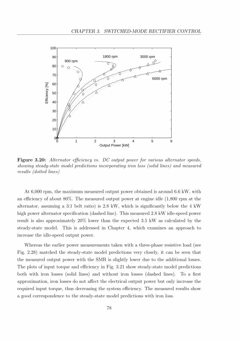
CHAPTER 3. SWITCHED-MODE RECTIFIER CONTROL
0 1 2 3 4 5 60
10
20
30
40
50
60
70
80
90
100
Output Power [kW]
Effi
cien
cy [%
]
900 rpm 1800 rpm 3000 rpm
6000 rpm
Figure 3.20: Alternator efficiency vs. DC output power for various alternator speeds,showing steady-state model predictions incorporating iron loss (solid lines) and measuredresults (dotted lines)
At 6,000 rpm, the maximum measured output power obtained is around 6.6 kW, with
an efficiency of about 80%. The measured output power at engine idle (1,800 rpm at the
alternator, assuming a 3:1 belt ratio) is 2.8 kW, which is significantly below the 4 kW
high power alternator specification (dashed line). This measured 2.8 kW idle-speed power
result is also approximately 20% lower than the expected 3.5 kW as calculated by the
steady-state model. This is addressed in Chapter 4, which examines an approach to
increase the idle-speed output power.
Whereas the earlier power measurements taken with a three-phase resistive load (see
Fig. 2.28) matched the steady-state model predictions very closely, it can be seen that
the measured output power with the SMR is slightly lower due to the additional losses.
The plots of input torque and efficiency in Fig. 3.21 show steady-state model predictions
both with iron losses (solid lines) and without iron losses (dashed lines). To a first
approximation, iron losses do not affect the electrical output power but only increase the
required input torque, thus decreasing the system efficiency. The measured results show
a good correspondence to the steady-state model predictions with iron loss.
78
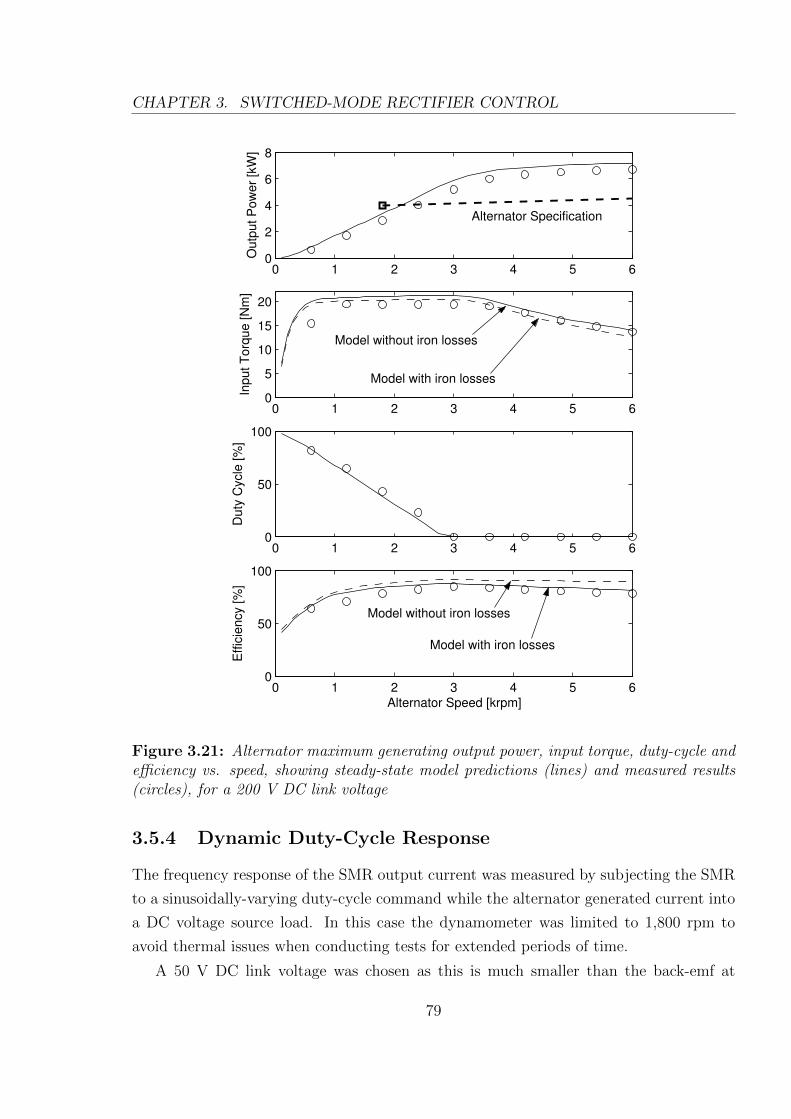
CHAPTER 3. SWITCHED-MODE RECTIFIER CONTROL
0 1 2 3 4 5 60
2
4
6
8
Alternator Specification
Outp
ut P
ow
er
[kW
]
0 1 2 3 4 5 60
5
10
15
20
Model without iron losses
Model with iron losses
Input T
orq
ue [N
m]
0 1 2 3 4 5 60
50
100
Duty
Cycle
[%
]
0 1 2 3 4 5 60
50
100
Model without iron losses
Model with iron losses
Alternator Speed [krpm]
Effic
iency [%
]
Figure 3.21: Alternator maximum generating output power, input torque, duty-cycle andefficiency vs. speed, showing steady-state model predictions (lines) and measured results(circles), for a 200 V DC link voltage
3.5.4 Dynamic Duty-Cycle Response
The frequency response of the SMR output current was measured by subjecting the SMR
to a sinusoidally-varying duty-cycle command while the alternator generated current into
a DC voltage source load. In this case the dynamometer was limited to 1,800 rpm to
avoid thermal issues when conducting tests for extended periods of time.
A 50 V DC link voltage was chosen as this is much smaller than the back-emf at
79

CHAPTER 3. SWITCHED-MODE RECTIFIER CONTROL
1,800 rpm and so allows for a larger range over which the output current to duty-cycle
characteristic is linear (see Fig. 3.22).
0 10 20 30 40 50 60 70 80 90 1000
5
10
15
20
25
30
35
Duty−Cycle [%]
DC
Outp
ut C
urr
ent [A
]
50 V
100 V
150 V
200 V
Figure 3.22: Calculated DC output current (lines) vs. duty cycle at 1,800 rpm forvarious DC link voltages, with measured current (circles) for a 50 V DC link.
To measure the duty-cycle frequency response, the MSA0654 microcontroller was pro-
grammed to accept a 0 - 5 V input voltage and generate a PWM waveform with a duty-
cycle dependent on the input voltage. The PWM output from the microcontroller was
set to have lower and upper duty-cycle limits of 55% and 75% respectively. This range
was chosen because the output current to duty-cycle response of the alternator and SMR
system was more linear towards higher duty-cycles. These duty-cycle limits correspond
to output current commands of 16 A and 9 A respectively (see Fig. 3.22). A sinusoidal
voltage from a signal generator was fed to the microcontroller in order to obtain a PWM
signal with a sinusoidally-varying duty-cycle, which was then used as the control input
to the SMR switch. A 4 kHz PWM frequency was used and the SMR output current
waveform was recorded for various input signal frequencies from 1 Hz to 700 Hz, in order
to measure the frequency response of the system.
An example measurement of the input signal and alternator output current waveform
is shown in Fig. 3.23, at a frequency of 200 Hz. The input duty-cycle sinusoid has an
amplitude of 12% duty, which corresponds to an expected output current amplitude of
3.45 A, however the observed output current amplitude is only about 2 A at this frequency.
Figure 3.24 shows plots of the system gain (ratio of output current amplitude to the
expected amplitude) and the phase difference between the output and the input. The gain
80

CHAPTER 3. SWITCHED-MODE RECTIFIER CONTROL
input duty-cycle output current
5% duty
1 ms
5 A
Figure 3.23: Duty-cycle command with a frequency of 200 Hz and corresponding alter-nator output current waveform (averaged signals shown)
−40
−30
−20
−10
0
Mag
nitu
de (d
B)
101
102
103
104
−180
−135
−90
−45
0
Pha
se (d
eg)
Fitted ResponseMeasured Results
Frequency (rad/sec)
Figure 3.24: Measured open-loop frequency response (circles) and fitted curves (lines)for the alternator and SMR at 1,800 rpm with a 50 V DC link voltage
response of the system remains flat up to a corner frequency of around 600rad/s (95 Hz).
The system transfer function was approximated by fitting a second-order response to the
81

CHAPTER 3. SWITCHED-MODE RECTIFIER CONTROL
measured results, giving the following open-loop system transfer function G(s), with a
double pole at 1200 rad/s:
G(s) =12002
(s+ 1200)2(3.3)
From (3.2) and (3.3), the complete open-loop response of the alternator output current
to duty-cycle can be described by (3.4):
IOUT = 36 · d′ · 12002
(s+ 1200)2, where d′ = (1− d) (3.4)
A Simulink model incorporating the transfer function G(s) was developed to predict
the dynamic response of the alternator output current.
As a simple validation of the model, Fig. 3.25 compares the alternator step response
predicted by the model to the experimentally measured waveform. The experimental
waveform was obtained by applying a periodic step change between 80% and 90% duty-
cycle to the SMR switch while the alternator was generating at 1,800 rpm into a DC
voltage source load of 50 V. As expected from Fig. 3.22, as the duty-cycle changes from
80% to 90%, the output current changes from 7.2 A to 3.6 A respectively. Although the
steady-state output matches the predictions, the time constant predicted by simulation
appears slightly longer than the measured time constant. Note that there is a 600 Hz
ripple modulated onto the current waveform. This is due to the three-phase rectifier,
which causes a ripple of six times the electrical frequency of the machine. There is also a
4 kHz ripple corresponding to the switching frequency of the SMR.
The mismatch in the predicted time constant suggests that the measured open-loop
frequency response is inaccurate. The reason for this discrepancy is unknown but for the
purpose of controller design, a transfer function with double poles at 4000 rad/s instead
of 1200 rad/s was used, which provides an output consistent with the measured step
response.
3.6 Controller Design and Implementation
The purpose of the closed-loop controller is to regulate the output voltage of the alternator.
This is achieved by adjusting the duty-cycle of the SMR switch in order to control the
output current flowing to the load. It was decided to design a proportional controller
to control the closed loop system, as represented in Fig. 3.26. This system could then
82
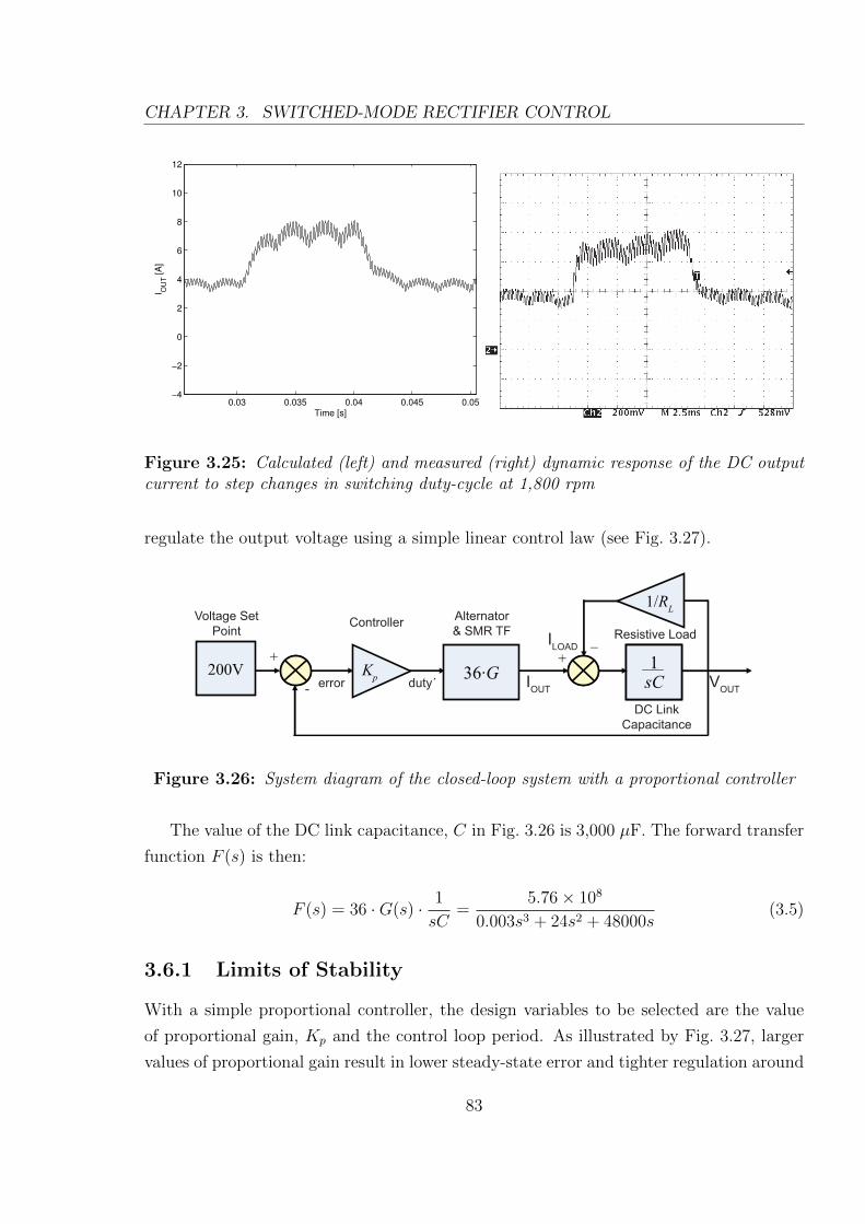
CHAPTER 3. SWITCHED-MODE RECTIFIER CONTROL
0.03 0.035 0.04 0.045 0.05−4
−2
0
2
4
6
8
10
12
Time [s]
I OU
T [A
]
Figure 3.25: Calculated (left) and measured (right) dynamic response of the DC outputcurrent to step changes in switching duty-cycle at 1,800 rpm
regulate the output voltage using a simple linear control law (see Fig. 3.27).
200V Kp
-
+
36·G1
sC1
sC
+−
1/RL
ControllerAlternator
& SMR TF
Voltage Set
PointILOAD
IOUT
duty´error VOUT
DC Link
Capacitance
Resistive Load
Figure 3.26: System diagram of the closed-loop system with a proportional controller
The value of the DC link capacitance, C in Fig. 3.26 is 3,000 µF. The forward transfer
function F (s) is then:
F (s) = 36 ·G(s) · 1
sC=
5.76× 10⁸
0.003s3 + 24s2 + 48000s(3.5)
3.6.1 Limits of Stability
With a simple proportional controller, the design variables to be selected are the value
of proportional gain, Kp and the control loop period. As illustrated by Fig. 3.27, larger
values of proportional gain result in lower steady-state error and tighter regulation around
83

CHAPTER 3. SWITCHED-MODE RECTIFIER CONTROL
194 196 198 200 202 204 2060
20
40
60
80
100
DC Output Voltage [V]
SM
R D
uty
−C
ycle
[%
]
Kp = 0.1
0.2
0.25
Figure 3.27: Linear control law for the controller, for various values of proportionalgain, Kp
the voltage set point, however the maximum allowable gain is constrained by the limits
of stability of the system.
The frequency response of F (s) is shown in Fig. 3.28. The combined phase delay
imposed by the alternator and the DC link capacitance causes the phase of the closed-
loop system to exceed -180at a frequency lower than the gain crossover frequency. The
gain margin, Gm is -3.52 dB, indicating that for stability, the gain should be at least 1.5
times smaller than unity, i.e. a stability threshold of Kp = 0.67.
The loop period or sampling time Ts of the digital controller affects how quickly
the controller responds to changes in the system. As the sampling time increases, the
bandwidth decreases, which means that the controller responds more slowly to output
voltage changes. It was decided that rather than setting the sampling time through the
timing of an interrupt routine, the Mitsubishi microcontroller would be allowed to iterate
through the control loop continuously in order to obtain the best possible performance.
The time taken to execute one iteration of the control loop was measured to be 284 µs.
Figure 3.29 shows the general shape of the discrete root locus plot of the alternator
open-loop system with a sampling time of 284 µs. The area of interest is the region which
is within the unit circle as these represent values of proportional gain which produce a
stable system. A close-up of this area is shown in Fig. 3.30, where loci for sampling times
of 80, 284 and 800 µs are also plotted. It can be seen that as sampling time increases,
the complex poles move towards the origin. This causes the oscillatory mode associated
84

CHAPTER 3. SWITCHED-MODE RECTIFIER CONTROL
−100
−50
0
50
100
Mag
nitu
de (d
B)
101
102
103
104
105
−270
−225
−180
−135
−90
Pha
se (d
eg)
Bode DiagramGm = −8.71 dB (at 2.2e+003 rad/sec) , Pm = −25.1 deg (at 3.46e+003 rad/sec)
Frequency (rad/sec)
Figure 3.28: Calculated open-loop frequency response of the interior PM alternator andSMR, showing gain and phase margins
with the complex poles to decay faster, however this also decreases the maximum stable
proportional gain, meaning that there is a trade-off between shorter settling time and
smaller steady-state error. For the case of a sampling time of 284 µs, a proportional gain
of greater than approximately 0.015 produces complex poles, while a gain of greater than
0.15 is unstable.
The closed-loop proportional gain is generally chosen to satisfy the steady-state error
requirement of the system. For example, the 42 V specification demands steady-state
variation not exceeding an upper limit of 50 V and a lower limit of 30 V. For the purpose
of comparison, this range represents 47.6% of the nominal voltage. A proportional gain
of Kp = 0.1 was chosen for the closed-loop controller, providing regulation of the DC
link voltage between 195 V and 205 V as the duty-cycle changes between 0% and 100%
respectively. This corresponds to a range of 5% of the nominal voltage, satisfying the
steady-state specification. The root locus plot indicates that this gain should give a
stable response, although the complex poles would result in some underdamped response
to input transients.
85

CHAPTER 3. SWITCHED-MODE RECTIFIER CONTROL
−10 −8 −6 −4 −2 0 2−6
−4
−2
0
2
4
6
Root Locus
Real Axis
Ima
gin
ary
Axis
Figure 3.29: Calculated discrete root locus plot of the open-loop system with a samplingperiod of 284 µs
0.6 0.65 0.7 0.75 0.8 0.85 0.9 0.95 1 1.05 1.1−0.2
−0.1
0
0.1
0.2
0.3
0.4
0.5
0.6
Root Locus
Real Axis
Imagin
ary
Axis
284µs 800µs
80µs
0.01 0.02
0.05
0.1
0.15
0.25
Figure 3.30: Enlarged view showing root loci for various values of sampling time Ts,with values of proportional gain shown at various points on the locus for sampling timeTs = 284 µs
86

CHAPTER 3. SWITCHED-MODE RECTIFIER CONTROL
3.6.2 Simulation
A dynamic model was developed in Simulink to predict the transient behaviour of the
closed-loop alternator and SMR system. The model incorporated the effects of microcon-
troller loop delay and voltage signal quantisation due to analogue-to-digital conversion.
Several test cases were tried on the control loop model to examine its stability and to
observe its response to various stimuli such as load changes and startup transients. These
results are shown in comparison with actual experimental measurements in the following
section.
87
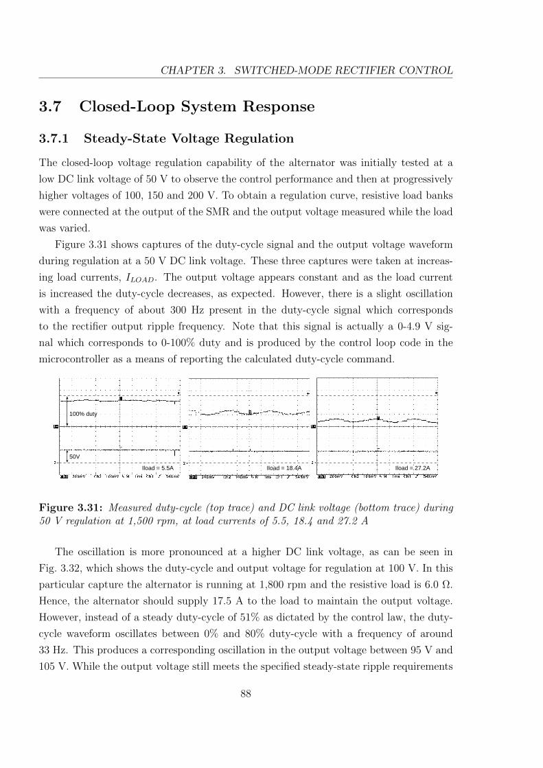
CHAPTER 3. SWITCHED-MODE RECTIFIER CONTROL
3.7 Closed-Loop System Response
3.7.1 Steady-State Voltage Regulation
The closed-loop voltage regulation capability of the alternator was initially tested at a
low DC link voltage of 50 V to observe the control performance and then at progressively
higher voltages of 100, 150 and 200 V. To obtain a regulation curve, resistive load banks
were connected at the output of the SMR and the output voltage measured while the load
was varied.
Figure 3.31 shows captures of the duty-cycle signal and the output voltage waveform
during regulation at a 50 V DC link voltage. These three captures were taken at increas-
ing load currents, ILOAD. The output voltage appears constant and as the load current
is increased the duty-cycle decreases, as expected. However, there is a slight oscillation
with a frequency of about 300 Hz present in the duty-cycle signal which corresponds
to the rectifier output ripple frequency. Note that this signal is actually a 0-4.9 V sig-
nal which corresponds to 0-100% duty and is produced by the control loop code in the
microcontroller as a means of reporting the calculated duty-cycle command.
100% duty
50V
Iload = 5.5A Iload = 18.4A Iload = 27.2A
Figure 3.31: Measured duty-cycle (top trace) and DC link voltage (bottom trace) during50 V regulation at 1,500 rpm, at load currents of 5.5, 18.4 and 27.2 A
The oscillation is more pronounced at a higher DC link voltage, as can be seen in
Fig. 3.32, which shows the duty-cycle and output voltage for regulation at 100 V. In this
particular capture the alternator is running at 1,800 rpm and the resistive load is 6.0 Ω.
Hence, the alternator should supply 17.5 A to the load to maintain the output voltage.
However, instead of a steady duty-cycle of 51% as dictated by the control law, the duty-
cycle waveform oscillates between 0% and 80% duty-cycle with a frequency of around
33 Hz. This produces a corresponding oscillation in the output voltage between 95 V and
105 V. While the output voltage still meets the specified steady-state ripple requirements
88
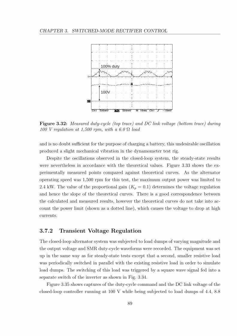
CHAPTER 3. SWITCHED-MODE RECTIFIER CONTROL
100% duty
100V
Figure 3.32: Measured duty-cycle (top trace) and DC link voltage (bottom trace) during100 V regulation at 1,500 rpm, with a 6.0 Ω load
and is no doubt sufficient for the purpose of charging a battery, this undesirable oscillation
produced a slight mechanical vibration in the dynamometer test rig.
Despite the oscillations observed in the closed-loop system, the steady-state results
were nevertheless in accordance with the theoretical values. Figure 3.33 shows the ex-
perimentally measured points compared against theoretical curves. As the alternator
operating speed was 1,500 rpm for this test, the maximum output power was limited to
2.4 kW. The value of the proportional gain (Kp = 0.1) determines the voltage regulation
and hence the slope of the theoretical curves. There is a good correspondence between
the calculated and measured results, however the theoretical curves do not take into ac-
count the power limit (shown as a dotted line), which causes the voltage to drop at high
currents.
3.7.2 Transient Voltage Regulation
The closed-loop alternator system was subjected to load dumps of varying magnitude and
the output voltage and SMR duty-cycle waveforms were recorded. The equipment was set
up in the same way as for steady-state tests except that a second, smaller resistive load
was periodically switched in parallel with the existing resistive load in order to simulate
load dumps. The switching of this load was triggered by a square wave signal fed into a
separate switch of the inverter as shown in Fig. 3.34.
Figure 3.35 shows captures of the duty-cycle command and the DC link voltage of the
closed-loop controller running at 100 V while being subjected to load dumps of 4.4, 8.8
89

CHAPTER 3. SWITCHED-MODE RECTIFIER CONTROL
0 5 10 15 20 25 30 350
50
100
150
200
250
1,500rpm Max. Power Limit
Load Current [A]
DC
Ou
tpu
t V
olta
ge
[V
]Theoretical CurvesMeasured Results
Figure 3.33: Closed-loop voltage regulation vs. load current at 1,500 rpm, for DC linkvoltages of 50, 100, 150 and 200 V
VDC
+
-
three-phaserectifier
switched-moderectifier
d
load dumpresistances
interior PMmachine
Vline
Iphase
RDUMP
RL1
IIN
VDC
IOUT
Microcontroller
RL2
Figure 3.34: Experimental configuration for closed-loop load dump tests
and 12.3 A. It can be seen that the overvoltage peak is small enough that it is only readily
discerned in the 12.3 A load dump. In these cases, the peak voltage reached was 110 V, i.e.
110% of nominal voltage, which is within the 42 V specification for maximum transient
overvoltage. This minimal overshoot is in accordance with what should be expected given
the short control loop period of 284 µs. The time required for the overvoltage to settle to
steady-state level was approximately 20 ms.
The measured waveforms differ notably from the simulated waveforms, particularly at
90

CHAPTER 3. SWITCHED-MODE RECTIFIER CONTROL
lower duty-cycles, where the oscillations previously observed in the steady-state regulation
are once again present in the measured waveform. While the simulated waveforms exhibit
a slight ripple which increases in amplitude at lower duty-cycles, no large oscillations are
present. The oscillations do not seem to have any impact on the load dump transient
response since they do not manifest for the high duty-cycles which are applied to limit
overvoltage.
The DC link was reduced from its nominal value of 200 V (corresponding to the 135 V
machine rating) to 100 V to reduce the risk of causing an over-voltage on the DC link
during the testing. The results obtained are effectively scaled versions of what would be
obtained in a 42 V system.
500 1000 15000
50
100
Dut
y [%
]
500 1000 150060
80
100
120
Vol
tage
[V]
Time [ms]
500 1000 15000
50
100
Dut
y [%
]
500 1000 150060
80
100
120
Vol
tage
[V]
Time [ms]
500 1000 15000
50
100
Dut
y [%
]
500 1000 150060
80
100
120
Vol
tage
[V]
Time [ms]
(a) 4.4A (b) 8.8A (c) 12.3A
100V
100% duty
Figure 3.35: Simulated (upper) and measured (lower) duty-cycle and DC link volt-age waveforms showing the load-dump response of the closed-loop system operating at1,800 rpm with a 100 V DC link
3.8 Summary of Findings
This chapter has investigated the control and performance of an inverterless interior PM
alternator based on a switched-mode rectifier. A simple closed-loop control system was
91

CHAPTER 3. SWITCHED-MODE RECTIFIER CONTROL
designed and the performance evaluated in terms of stability, transient voltage suppression
and output voltage regulation versus load. The main findings are:
• A simple proportional controller is capable of regulating the alternator steady-state
output voltage. Results show a 1% decrease in output voltage for 25% increase in
load current, which is within the specified steady-state range of 48% of nominal
voltage.
• The maximum overvoltage produced by the closed-loop system in response to a load
current step of 8.8 A, representing an 880 W load dump, was 10 V. The load dump
transient settled to its steady-state value after roughly 20 ms. The peak value is
110% of the nominal output voltage, which is well below the 42 V specification of
138%.
In summary, the closed-loop inverterless alternator shows promising performance as
an automotive alternator, with indications that it will be able to satisfy the high power
alternator specifications. However, further work is required in some areas:
• The controller duty-cycle exhibits oscillations which increase in amplitude as load
current increases. These cause a corresponding output voltage ripple. Some possible
causes are non-linearity in the output current response, mechanical oscillations, or
digital control loop limitations.
• The open-loop transfer function derived from the measured frequency response of
the alternator predicts an output current frequency response with a larger time
constant than exhibited by a measured step response. This needs to be further
investigated as both measurements were taken under similar conditions.
• With regards to the suppression of load dump overvoltage transients, more severe
tests should be attempted. It would however be prudent to first address the issue
of controller oscillations so that the mechanical effect on the dynamometer rig is
minimised.
92
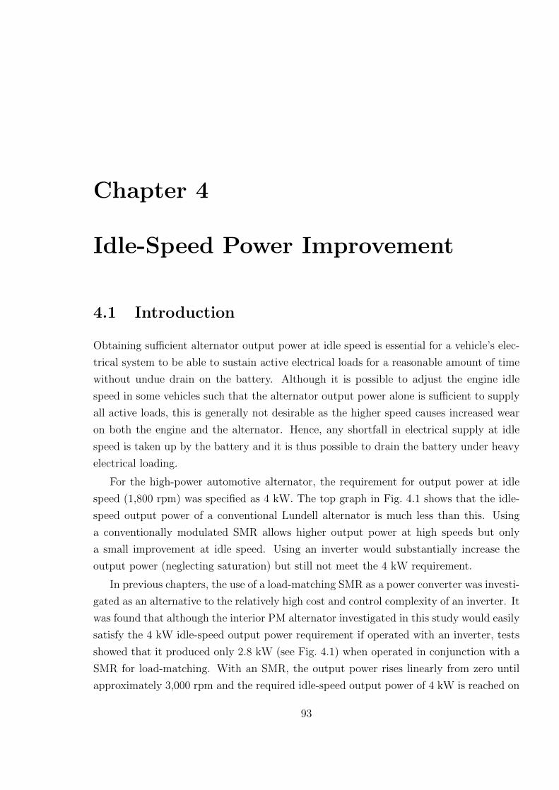
Chapter 4
Idle-Speed Power Improvement
4.1 Introduction
Obtaining sufficient alternator output power at idle speed is essential for a vehicle’s elec-
trical system to be able to sustain active electrical loads for a reasonable amount of time
without undue drain on the battery. Although it is possible to adjust the engine idle
speed in some vehicles such that the alternator output power alone is sufficient to supply
all active loads, this is generally not desirable as the higher speed causes increased wear
on both the engine and the alternator. Hence, any shortfall in electrical supply at idle
speed is taken up by the battery and it is thus possible to drain the battery under heavy
electrical loading.
For the high-power automotive alternator, the requirement for output power at idle
speed (1,800 rpm) was specified as 4 kW. The top graph in Fig. 4.1 shows that the idle-
speed output power of a conventional Lundell alternator is much less than this. Using
a conventionally modulated SMR allows higher output power at high speeds but only
a small improvement at idle speed. Using an inverter would substantially increase the
output power (neglecting saturation) but still not meet the 4 kW requirement.
In previous chapters, the use of a load-matching SMR as a power converter was investi-
gated as an alternative to the relatively high cost and control complexity of an inverter. It
was found that although the interior PM alternator investigated in this study would easily
satisfy the 4 kW idle-speed output power requirement if operated with an inverter, tests
showed that it produced only 2.8 kW (see Fig. 4.1) when operated in conjunction with a
SMR for load-matching. With an SMR, the output power rises linearly from zero until
approximately 3,000 rpm and the required idle-speed output power of 4 kW is reached on
93
CHAPTER 4. IDLE-SPEED POWER IMPROVEMENT
this slope at 2,400 rpm.
0 1.8 180
2
4
6
8
Speed [krpm]
Out
put P
ower
[kW
]
inverter specification
SMR
rectifier
a) Lundell Alternator
0 1.8 180
2
4
6
8
Speed [krpm]
Out
put P
ower
[kW
]
inverter
specification SMR test
b) Interior PM Alternator
SMR
SMR test2.8 kW at idle
Figure 4.1: Output power versus speed characteristics for an example a) Lundell andb) interior PM alternator using different power electronics topologies, showing calculatedcurves (lines) and test data using a SMR (circles)
It is the presence of two controllable switches on all phase legs of an inverter which
allows better optimisation of output power as compared to a single-switch SMR and
there have been several studies which make use of the added flexibility of such controlled
rectifiers to improve alternator output power. Liang et al. applied six-step waveform
modulation using an inverter to achieve an increase of 43% in the idle-speed output
power of a Lundell alternator [28]. Kikuchi, Manjrekar and Lipo carried out a detailed
analysis of the operation of the semi-bridge rectifier for improving the shape of the input
current waveform compared to an uncontrolled rectifier in a motor drive [40].
In terms of control flexibility, the semi-bridge SMR with its three controllable switches
can be considered an intermediate step between an inverter and a single-switch SMR and
94

CHAPTER 4. IDLE-SPEED POWER IMPROVEMENT
recent work by Rivas, Perreault and Keim [15] on a semi-bridge SMR modulation scheme
achieved a 15% increase in output power of a Lundell alternator at idle speed.
In this chapter, the difference in the operation and output power capability of an
inverter and a conventional single-switch SMR is discussed. The SMR modulation scheme
proposed by Rivas, Perreault and Keim for a semi-bridge SMR is examined and the way
in which it improves the output power at low speeds is discussed. The application of
the modulation scheme to the interior PM alternator and the resulting output power
performance is theoretically investigated and simulated models are constructed. The
modulation scheme is implemented on a microcontroller and experimental results are
obtained.
4.2 Power Converters
4.2.1 Single-Switch SMR and Inverter Low-Speed Performance
The purpose of a power converter in an automotive alternator system is to convert AC
input power to DC output power with high efficiency. At any speed, the converter should
maximise output power while not exceeding the rated output voltage and current of the
alternator. The output power of an alternator can be expressed as the product of its
voltage, current and power-factor (4.1). These quantities are in turn dependent on the
load to which the alternator is connected and the operating speed. Neglecting voltage
or current limits, optimum power transfer is obtained with a matched load, i.e. a load
with an impedance which is the conjugate to the alternator output impedance. When
comparing alternator operation using a SMR as opposed to an inverter, the difference
in performance is due to the extent to which each converter is capable of adjusting the
effective load impedance and power factor seen by the alternator to maximise the output
power.
P = V I cosφ (4.1)
As depicted in Fig. 4.2, to a first approximation the alternator has a purely inductive
output impedance, Xs. In order to extract the optimal power, a load with a leading power
factor needs to be applied. Although the single-switch SMR can adjust the magnitude of
its input impedance by varying the switching duty-cycle, the input rectifier of the SMR
forces the alternator phase voltage and current to be in phase and thus the alternator
95

CHAPTER 4. IDLE-SPEED POWER IMPROVEMENT
is constrained to operate at unity power-factor. The SMR can therefore be considered
a variable purely resistive load. In comparison, the control flexibility afforded by the
additional switches in an inverter allows both its input impedance and power-factor to
be varied. The inverter can therefore be modelled by a variable passive RC load. In
a previous study [16], an RC load was in fact used to extract maximum power from
the interior PM alternator, thus simulating the alternator performance delivered by an
inverter. Figure 4.3 shows the calculated parallel three-phase resistances and capacitances
required to simulate inverter operation with maximum output power without exceeding
the rated voltage or current of the machine. Note the load resistance is fairly constant
but the required capacitance falls rapidly with speed.
Consider in Fig. 4.2 the speed corresponding to the ’knee’ in the inverter voltage
versus speed characteristic (leftmost vertical dashed line). At this speed, both the inverter
voltage and current are at their rated values (1 pu), the power-factor is optimum at 0.7
leading and hence the inverter output power is 1 pu x 1 pu x 0.7 = 0.7 pu. With the
SMR at the same operating speed, the unity power-factor constraint means that at the
maximum output power operating point the output current is only 0.7 pu and the output
voltage is only 0.5 pu. The SMR output power is then 0.5 pu x 0.7 pu x 1 = 0.35 pu, or
half the inverter output power.
It can be seen that at low speeds, the inverter can supply the required load impedance
and input power-factor (0.7 leading) to maintain rated output current and so extracts
twice the power achievable with a SMR at that speed. At high speeds, the optimal
power-factor approaches unity and hence the output powers obtained with both SMR
and inverter are comparable.
4.2.2 Proposed Semi-Bridge SMR Modulation Scheme
In the proposed semi-bridge SMR modulation scheme, the PWM duty-cycle is modulated
to control the effective voltage applied to each phase. Since only the lower switch in
each phase of the semi-bridge SMR is used, the voltage can only be controlled during the
positive half-cycle of the phase current. When the phase current is positive, controlling
the duty-cycle d of the switch controls the effective phase to ground voltage VEFF applied
to the phase, where the effective voltage VEFF = VDC(1 − d) and VDC is the DC link
voltage. When the phase current is negative, the lower phase leg diode conducts. The
effective voltage is zero and is independent of the switch duty-cycle. This is illustrated
in Fig. 4.4, which shows that a time-varying phase A effective voltage during the phase
96

CHAPTER 4. IDLE-SPEED POWER IMPROVEMENT
voltageinverter
1puSMR
speed0
currentinverter
1puSMR
speed0
power
Inverter Operation
SMR Operation
inverter1pu
SMR
speed0
p.f.SMR
1puinverter
speed0
I ≤ 1pu V ≤ 1puXS
R C
I ≤ 1pu V ≤ 1puXS
R
Figure 4.2: Comparison of SMR and inverter operation: the SMR acts as a resistiveload with fixed unity power factor while the inverter produces a controllable power-factorallowing it to extract more power at low speeds
A positive current half-cycle is obtained by appropriately changing the duty-cycle. Note
that for the conventional load-matching SMR operation, a constant value of duty-cycle
and hence effective voltage would be used on all phases.
The proposed modulation scheme divides the positive half-cycle of the phase current
waveform into three intervals - a first interval δ where VEFF is set to a low value allowing
the current to build up rapidly, a second interval ε during which VEFF is set to VBASE in
order to achieve the normal load-matching condition and a third interval φ, during which
VEFF is increased by the amount VOV in order to force the current down rapidly. These
differing levels of VEFF are obtained by modulating the duty-cycle of each phase-leg switch
appropriately. The switching signals to each phase are identical but shifted by 120 from
each other, as shown in Fig. 4.5.
97

CHAPTER 4. IDLE-SPEED POWER IMPROVEMENT
Figure 4.3: Three-phase parallel resistance and capacitance per phase used to producethe ”inverter” maximum output power characteristics [16]
The effect of the modulation scheme can be viewed as a change in the magnitude and
phase of the fundamental of VEFF , in a similar manner as was investigated in [40]. The
presence of the δ interval at the beginning of the positive current half-cycle both increases
the current amplitude and shifts the fundamental of the VEFF waveform later in time,
causing the phase current to lead VEFF . This leading phase shift is similar to that obtained
with an inverter and so the semi-bridge SMR operating under this modulation scheme thus
represents an intermediate step between the single-switch SMR and the inverter which
utilises six switches. The additional control flexibility offered over a single-switch SMR
allows the operating power-factor to be adjusted to increase output power. However, it
is expected that the maximum achievable power with this scheme will be less than that
obtained with an inverter. Additionally, due to the asymmetry in the semi-bridge SMR,
the phase current waveforms will be distorted.
4.3 Simulation Studies
The steady-state d− q model of the interior PM alternator described in previous chapters
was used to examine and contrast the performance of the interior PM machine under in-
verter operation with the performance under conventional single-switch SMR operation.
A time-stepping dynamic model of the semi-bridge SMR modulation scheme was devel-
98
A NOTE:
This figure/table/image has been removed to comply with copyright regulations. It is included in the print copy of the thesis held by the University of Adelaide Library.
CHAPTER 4. IDLE-SPEED POWER IMPROVEMENT
Figure 4.4: Diagram illustrating modulation scheme intervals in relation to phase currentand effective voltage [15]
oped to simulate the response of the interior PM alternator over the modulation scheme
parameter space in order to explore the potential output power improvement and key
trends.
In all cases, the calculations were carried out for the idle speed of 1,800 rpm, using
a DC link voltage of 200 V which corresponds to an effective machine AC line voltage
of 156 V. The steady-state and dynamic models incorporated the effects of magnetic
saturation and stator resistance.
4.3.1 Inverter Control versus Conventional SMR Control
Figure 4.6 examines the calculated operating trajectories in the d − q current plane of
SMR operation and inverter operation both with and without a voltage limit. The rated
current limit circle and voltage limit ellipse are shown for reference. The operating curve
for the inverter without a voltage limit corresponds closely to the maximum torque per
ampere operating line. Without saturation this would be expected to follow a 45 slope
at high currents, however the heavy saturation in this machine causes the slope to be
lower. The voltage-limited inverter trajectory is shown as a bold line. This curve departs
from the maximum torque per ampere trajectory when it reaches the voltage limit ellipse
and is constrained to follow this ellipse at higher currents. The SMR operating curve is
restricted to a smaller ellipse, associated with its unity power-factor operation.
99
A NOTE:
This figure/table/image has been removed to comply with copyright regulations. It is included in the print copy of the thesis held by the University of Adelaide Library.
CHAPTER 4. IDLE-SPEED POWER IMPROVEMENT
Figure 4.5: Relationship between phase currents, phase effective voltage and gate drivesignals for the new modulation scheme (modified from [15])
Figures 4.7, 4.8 and 4.9 show the calculated output power, phase voltage and power-
factor versus current associated with the three trajectories shown in Fig. 4.6. It can be
seen in Fig. 4.7 that despite the large apparent difference between the d-q current plane
trajectories of inverter operation with and without a voltage limit, the output power
versus current curves do not show significant difference until above rated current. The
calculated output power with voltage-limited inverter operation at rated current (28 A)
is about 6.5 kW. For the SMR the maximum power of 3.6 kW occurs at about 20 A.
This is significantly less than rated current, so there is some leeway for the current to be
increased in order to improve the output power.
Figure 4.8 shows that the maximum torque per ampere inverter operation produces
a terminal voltage which is equal to the back-EMF voltage (≈65 V) at zero current
and increases with output current. The voltage-limited inverter operation alters the d-q
100
A NOTE:
This figure/table/image has been removed to comply with copyright regulations. It is included in the print copy of the thesis held by the University of Adelaide Library.

CHAPTER 4. IDLE-SPEED POWER IMPROVEMENT
−50 −40 −30 −20 −10 00
5
10
15
20
25
30
35
40
Id [Arms]
Iq [A
rms]
inverter : volt limited
inverter : no volt limit
current limit circle
voltage limit ellipse
SMR
Figure 4.6: Calculated d-q current plane operating trajectories for the SMR and theinverter with or without a voltage limit, operating at 1800 rpm with a DC link voltage of200 V
0 10 20 30 40 500
2
4
6
8
10
12
Phase Current [Arms]
Out
put P
ower
[kW
]
rated currentinverter : no volt limit
inverter : volt limited
SMR
6.5 kW
3.5 kW
Figure 4.7: Calculated output power versus phase current for the SMR and the inverterwith and without voltage limit
101

CHAPTER 4. IDLE-SPEED POWER IMPROVEMENT
0 10 20 30 40 500
20
40
60
80
100
120
Phase Current [Arms]
Pha
se V
olta
ge [V
rms]
rated current
inverter : no volt limit
inverter : volt limited
SMR
rated voltage
Figure 4.8: Calculated phase voltage versus phase current for the SMR and the inverterwith and without voltage limit
0 10 20 30 40 50
0.65
0.7
0.75
0.8
0.85
0.9
0.95
1
Phase Current [Arms]
Pow
er−
Fac
tor
SMR
inverter : no volt limit
inverter : volt limited
rated current
Figure 4.9: Calculated power factor versus phase current for the SMR and the inverterwith and without voltage limit
current plane trajectory to keep this within the voltage limit. With SMR operation the
generator phase voltage never reaches its rated value and falls rapidly at higher currents.
102
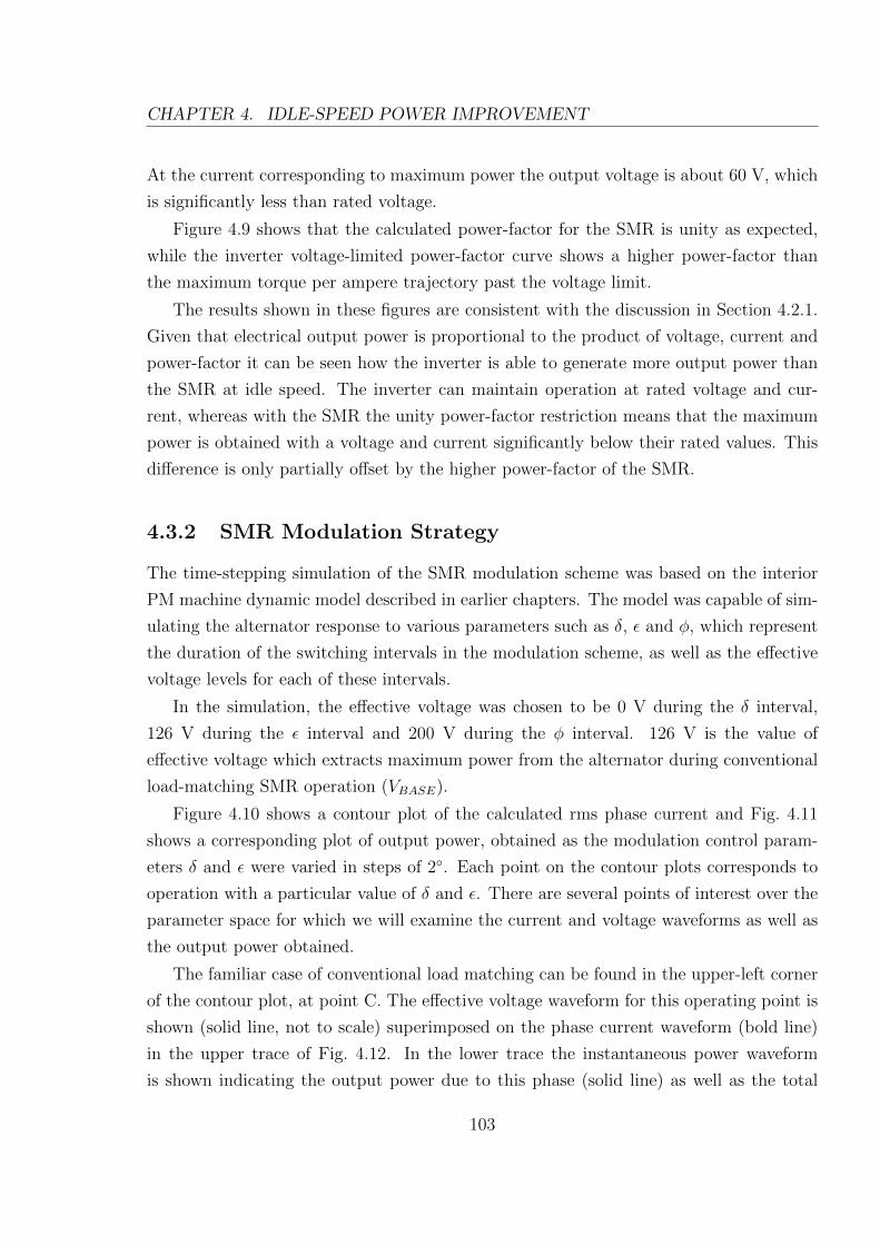
CHAPTER 4. IDLE-SPEED POWER IMPROVEMENT
At the current corresponding to maximum power the output voltage is about 60 V, which
is significantly less than rated voltage.
Figure 4.9 shows that the calculated power-factor for the SMR is unity as expected,
while the inverter voltage-limited power-factor curve shows a higher power-factor than
the maximum torque per ampere trajectory past the voltage limit.
The results shown in these figures are consistent with the discussion in Section 4.2.1.
Given that electrical output power is proportional to the product of voltage, current and
power-factor it can be seen how the inverter is able to generate more output power than
the SMR at idle speed. The inverter can maintain operation at rated voltage and cur-
rent, whereas with the SMR the unity power-factor restriction means that the maximum
power is obtained with a voltage and current significantly below their rated values. This
difference is only partially offset by the higher power-factor of the SMR.
4.3.2 SMR Modulation Strategy
The time-stepping simulation of the SMR modulation scheme was based on the interior
PM machine dynamic model described in earlier chapters. The model was capable of sim-
ulating the alternator response to various parameters such as δ, ε and φ, which represent
the duration of the switching intervals in the modulation scheme, as well as the effective
voltage levels for each of these intervals.
In the simulation, the effective voltage was chosen to be 0 V during the δ interval,
126 V during the ε interval and 200 V during the φ interval. 126 V is the value of
effective voltage which extracts maximum power from the alternator during conventional
load-matching SMR operation (VBASE).
Figure 4.10 shows a contour plot of the calculated rms phase current and Fig. 4.11
shows a corresponding plot of output power, obtained as the modulation control param-
eters δ and ε were varied in steps of 2. Each point on the contour plots corresponds to
operation with a particular value of δ and ε. There are several points of interest over the
parameter space for which we will examine the current and voltage waveforms as well as
the output power obtained.
The familiar case of conventional load matching can be found in the upper-left corner
of the contour plot, at point C. The effective voltage waveform for this operating point is
shown (solid line, not to scale) superimposed on the phase current waveform (bold line)
in the upper trace of Fig. 4.12. In the lower trace the instantaneous power waveform
is shown indicating the output power due to this phase (solid line) as well as the total
103

CHAPTER 4. IDLE-SPEED POWER IMPROVEMENT
0 30 60 90 120 150 1800
30
60
90
120
150
180
δ [deg]
ε [d
eg]
30
35 Arms
40
35
30
25
10545
20
C
B
G
FE D
A
Figure 4.10: Contour plot of calculated rms phase current versus modulation parametersδ and ε at 1,800 rpm, showing operating points of interest
three-phase instantaneous output power (dashed line). With a constant load-matching
VEFF of 126 V, the phase current of 20 A is sinusoidal and the total instantaneous output
power is relatively smooth and has an average value of 3.5 kW.
Operating point A corresponds to the short-circuit case where the δ interval takes up
the entire period (VEFF = 0 V). The phase current is equal to the short-circuit current of
27 A and the output power is zero (see Fig. 4.13).
Moving to the origin, point B corresponds to the open-circuit case, where VEFF =
200 V. This is greater than the back-EMF voltage at this speed, hence no current flows
and the power is again zero.
Assuming a symmetrical current waveform, δ + ε = 180, hence it is not possible
to operate in the upper-right half of the contour plots of Figures 4.10 and 4.11. The
operating points A, B and C which mark the three corners of the usable parameter space
represent conventional modes of operation. By varying the modulation parameters within
104

CHAPTER 4. IDLE-SPEED POWER IMPROVEMENT
0 30 60 90 120 150 1800
30
60
90
120
150
180
δ [deg]
ε [d
eg]
A
B
C
DE
F
G 1 kW2
34
5
6
4
21
5
Figure 4.11: Contour plot of calculated average output power (kW) versus modulationparameters δ and ε at 1,800 rpm
this space, it is possible to increase both the phase current and the output power. For
instance, the maximum value of phase current obtained is 46 A, at operating point D (see
Fig. 4.14). It can be seen that the current waveform has become less sinusoidal and the
instantaneous output power is highly discontinuous, with an average value of 4 kW.
The current obtained at point D greatly exceeds the 27 A rating of the alternator
and would involve excessive heat dissipation, with the associated increased risk of de-
magnetisation. Of perhaps more practical interest is the maximum power point, at E.
The output power obtained approaches 7 kW, achieved by keeping the effective voltage
at zero to build the current up and then using maximum bus voltage to extract as much
power as possible. The time domain waveforms corresponding to this case are shown in
Fig. 4.15, where a large ripple content can be observed in the instantaneous power wave-
form. The current is approximately 37 A, which is still significantly greater than rated
current. There is an interesting similarity between this type of control and that used for
105

CHAPTER 4. IDLE-SPEED POWER IMPROVEMENT
0.495 0.5 0.505 0.51 0.515
−50
0
50IPH
= 20.1 ArmsC
urre
nt [A
rms]
0.495 0.5 0.505 0.51 0.5150
5
10 PAVG
= 3.5 kW
Time [s]
Pow
er [k
W]
VEFF
IPH
Figure 4.12: Conventional SMR ’load-matching’ operation at point C (δ = 0, ε = 180)
0.495 0.5 0.505 0.51 0.515
−50
0
50IPH
= 27.4 Arms
Cur
rent
[Arm
s]
0.495 0.5 0.505 0.51 0.5150
5
10 PAVG
= 0 kW
Time [s]
Pow
er [k
W]
VEFF
IPH
Figure 4.13: Short-circuit operation at point A (δ = 180, ε = 0)
switched-reluctance machines and brushless DC machines at high speed.
The maximum power obtainable without exceeding rated current is 5.9 kW, which
can be found at point F (see Fig. 4.16). Note that in spite of the varying effective voltage
used to boost the current amplitude, the shape of the positive half-cycle of the waveform
is close to sinusoidal, indicating that the energy is still concentrated in the fundamental.
106

CHAPTER 4. IDLE-SPEED POWER IMPROVEMENT
0.495 0.5 0.505 0.51 0.515
−50
0
50 IPH
= 45.7 Arms
Cur
rent
[Arm
s]
0.495 0.5 0.505 0.51 0.5150
5
10
15
PAVG
= 3.96 kW
Time [s]
Pow
er [k
W]
VEFF
IPH
Figure 4.14: Maximum phase current obtained at point D (δ = 105, ε = 5)
0.495 0.5 0.505 0.51 0.515
−50
0
50IPH
= 36.8 Arms
Cur
rent
[Arm
s]
0.495 0.5 0.505 0.51 0.5150
5
10 PAVG
= 6.82 kW
Time [s]
Pow
er [k
W]
VEFF
IPH
Figure 4.15: Maximum power obtained at point E (δ = 60, ε = 0)
4.3.3 Optimal Operating Regions
Figure 4.18 shows a scatter plot of the simulation results illustrating the relationship
between output power and rms machine phase current. For reference, the calculated
allowable power versus current loci are shown for both a conventional SMR and an inverter
(from Fig. 4.7). This figure clearly shows that the modulation scheme allows much more
flexibility in the choice of operating points than the conventional SMR control scheme and
107
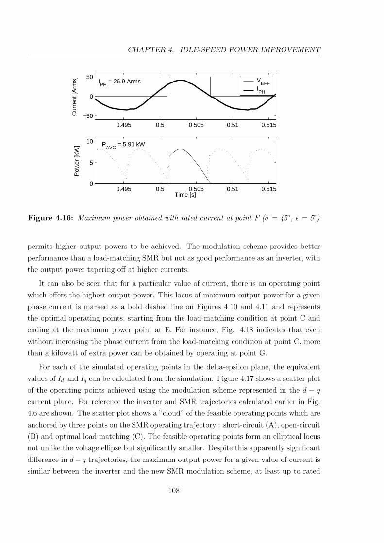
CHAPTER 4. IDLE-SPEED POWER IMPROVEMENT
0.495 0.5 0.505 0.51 0.515
−50
0
50IPH
= 26.9 ArmsC
urre
nt [A
rms]
0.495 0.5 0.505 0.51 0.5150
5
10 PAVG
= 5.91 kW
Time [s]
Pow
er [k
W]
VEFF
IPH
Figure 4.16: Maximum power obtained with rated current at point F (δ = 45, ε = 5)
permits higher output powers to be achieved. The modulation scheme provides better
performance than a load-matching SMR but not as good performance as an inverter, with
the output power tapering off at higher currents.
It can also be seen that for a particular value of current, there is an operating point
which offers the highest output power. This locus of maximum output power for a given
phase current is marked as a bold dashed line on Figures 4.10 and 4.11 and represents
the optimal operating points, starting from the load-matching condition at point C and
ending at the maximum power point at E. For instance, Fig. 4.18 indicates that even
without increasing the phase current from the load-matching condition at point C, more
than a kilowatt of extra power can be obtained by operating at point G.
For each of the simulated operating points in the delta-epsilon plane, the equivalent
values of Id and Iq can be calculated from the simulation. Figure 4.17 shows a scatter plot
of the operating points achieved using the modulation scheme represented in the d − qcurrent plane. For reference the inverter and SMR trajectories calculated earlier in Fig.
4.6 are shown. The scatter plot shows a ”cloud” of the feasible operating points which are
anchored by three points on the SMR operating trajectory : short-circuit (A), open-circuit
(B) and optimal load matching (C). The feasible operating points form an elliptical locus
not unlike the voltage ellipse but significantly smaller. Despite this apparently significant
difference in d− q trajectories, the maximum output power for a given value of current is
similar between the inverter and the new SMR modulation scheme, at least up to rated
108

CHAPTER 4. IDLE-SPEED POWER IMPROVEMENT
−50 −40 −30 −20 −10 00
5
10
15
20
25
30
35
Id [Arms]
Iq [A
rms]
SMR
F E G
D
A
C
B
Semi−bridge SMR
inverter : no volt limit
inverter : volt limitedvoltage limit
ellipse
current limit circle
Figure 4.17: Scatter plot of calculated feasible d-q currents available using the proposedSMR modulation scheme at 1,800 rpm, with key operating points indicated. Inverter andSMR operating trajectories are shown for reference.
current.
4.4 Experimental Setup
Experimental results were obtained using the dynamometer test rig set up as shown in
Fig. 4.19. The output of the interior PM alternator was fed through the semi-bridge SMR
into a 200 V DC voltage source load simulator consisting of a DC power supply, protective
diode and a resistive load bank. This arrangement maintains a constant DC link voltage
despite variations in the output current of the SMR, up to a maximum current equal to
the DC link voltage divided by the load resistance.
The modulation scheme was implemented on a Microchip dsPIC30F10 16-bit micro-
controller. Hall-effect current sensors present on each phase of the SMR provided phase
current signals to the modulation controller and the appropriate switching signals were de-
termined based on the modulation parameters. These were 5 kHz pulse-width-modulated
(PWM) signals which in turn controlled the lower phase-leg switches of the SMR.
109

CHAPTER 4. IDLE-SPEED POWER IMPROVEMENT
0 10 20 30 40 500
2
4
6
8
10
12
Phase Current [Arms]
Out
put P
ower
[kW
]
inverter : volt limited
SMR
Semi−bridge SMR
inverter : no volt limitrated current
BA
C
G
FE
D
Figure 4.18: Scatter plot of calculated output power versus phase current at 1,800 rpmwith key operating points indicated. The calculated performance with a SMR and a voltage-limited inverter is shown for reference.
VDC
+
-
three-phaserectifier
variabletransformer
240 Vmains
interior PMmachine
RDUMP
RLOADIc
Ib
Ia
Microcontroller
Figure 4.19: Experimental configuration for low-speed power improvement testing
In the experimental tests, the current sensors were only used for detecting the zero
crossings of the phase currents. This timing information can also be obtained using inex-
pensive phase-to-ground voltage sensors, thus eliminating the need for current sensors [15]
and it is expected that the implementation of the proposed modulation scheme in this
110
CHAPTER 4. IDLE-SPEED POWER IMPROVEMENT
way should result in only a small incremental cost over the conventional load matching
control.
The outputs from the current sensors were passed through op-amp Schmitt triggers
in order to obtain suitable digital signals. The edge transition of the waveform from a
low to a high level was used to trigger a micro-controller interrupt which executed the
code for the modulation scheme. The modulation controller was programmed to offer
real-time menu-based adjustment of the modulation parameters δ and ε via a digital
opto-interrupter control knob and buttons. The values of the modulation parameters
were displayed on a Liquid Crystal Display (LCD) module.
Appropriately placed meters were used to record the machine phase currents and line
voltages, as well as the current sensor outputs and the DC output current, IOUT delivered
to the load. The gate driver signal to one of the phase-leg switches was low-pass filtered
and inverted to provide an approximate representation of the effective voltage waveform
VEFF .
During tests, when the alternator was brought up from standstill to 1,800 rpm, the
modulation controller was kept at the conventional load-matching setting (point C in
Fig. 4.10). It was initially planned to incrementally adjust the modulation parameter
values via the control interface until the desired operating point was obtained. Although
it was found that the modulation controller parameters could be dynamically adjusted,
one of the issues encountered was that when the operating point was moved too far from
the load-matching point, the dynamometer rig produced significant torque vibrations and
oscillations in speed. Similar behaviour was also observed when an operating point was
attempted after bringing the alternator up to 1,800 rpm in short-circuit operation.
The modulation controller was then reprogrammed to allow for an instantaneous
switch between load-matching operation and the phase advance modulation scheme. It
was found that switching directly from load-matching to the desired operating point
caused no noticable problems with vibration. Once the operating point was achieved, the
parameter values could be adjusted to some degree around that point without causing
oscillations.
As the operating point shifts within the parameter space the alternator reaction torque
changes. The poor mechanical stiffness of the dynamometer rig allowed the operating
speed to fluctuate slightly with such changes. This, coupled with the fact that the mod-
ulation controller bases its timing off the zero-crossings of the phase current waveform, is
one possible cause of the observed oscillations.
111
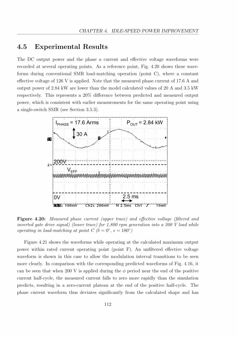
CHAPTER 4. IDLE-SPEED POWER IMPROVEMENT
4.5 Experimental Results
The DC output power and the phase a current and effective voltage waveforms were
recorded at several operating points. As a reference point, Fig. 4.20 shows these wave-
forms during conventional SMR load-matching operation (point C), where a constant
effective voltage of 126 V is applied. Note that the measured phase current of 17.6 A and
output power of 2.84 kW are lower than the model calculated values of 20 A and 3.5 kW
respectively. This represents a 20% difference between predicted and measured output
power, which is consistent with earlier measurements for the same operating point using
a single-switch SMR (see Section 3.5.3).
IPHASE = 17.6 Arms
30 A
VEFF
200V
2.5 ms
POUT = 2.84 kW
0V
IPHASE = 17.6 Arms
30 A
VEFF
200V
2.5 ms
POUT = 2.84 kW
0V
Figure 4.20: Measured phase current (upper trace) and effective voltage (filtered andinverted gate drive signal) (lower trace) for 1,800 rpm generation into a 200 V load whileoperating in load-matching at point C (δ = 0, ε = 180)
Figure 4.21 shows the waveforms while operating at the calculated maximum output
power within rated current operating point (point F). An unfiltered effective voltage
waveform is shown in this case to allow the modulation interval transitions to be seen
more clearly. In comparison with the corresponding predicted waveforms of Fig. 4.16, it
can be seen that when 200 V is applied during the φ period near the end of the positive
current half-cycle, the measured current falls to zero more rapidly than the simulation
predicts, resulting in a zero-current plateau at the end of the positive half-cycle. The
phase current waveform thus deviates significantly from the calculated shape and has
112
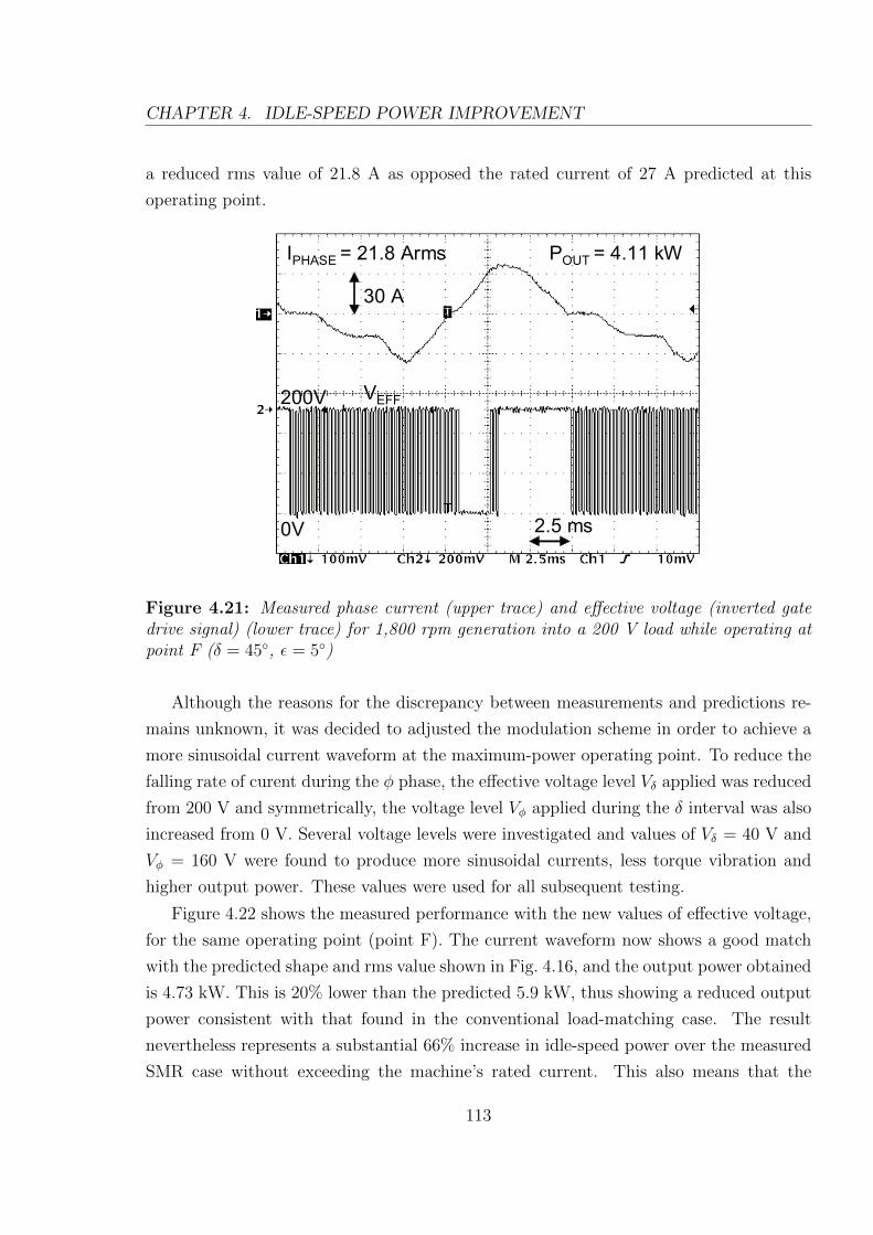
CHAPTER 4. IDLE-SPEED POWER IMPROVEMENT
a reduced rms value of 21.8 A as opposed the rated current of 27 A predicted at this
operating point.
IPHASE = 21.8 Arms
30 A
VEFF200V
0V 2.5 ms
POUT = 4.11 kWIPHASE = 21.8 Arms
30 A
VEFF200V
0V 2.5 ms
POUT = 4.11 kW
Figure 4.21: Measured phase current (upper trace) and effective voltage (inverted gatedrive signal) (lower trace) for 1,800 rpm generation into a 200 V load while operating atpoint F (δ = 45, ε = 5)
Although the reasons for the discrepancy between measurements and predictions re-
mains unknown, it was decided to adjusted the modulation scheme in order to achieve a
more sinusoidal current waveform at the maximum-power operating point. To reduce the
falling rate of curent during the φ phase, the effective voltage level Vδ applied was reduced
from 200 V and symmetrically, the voltage level Vφ applied during the δ interval was also
increased from 0 V. Several voltage levels were investigated and values of Vδ = 40 V and
Vφ = 160 V were found to produce more sinusoidal currents, less torque vibration and
higher output power. These values were used for all subsequent testing.
Figure 4.22 shows the measured performance with the new values of effective voltage,
for the same operating point (point F). The current waveform now shows a good match
with the predicted shape and rms value shown in Fig. 4.16, and the output power obtained
is 4.73 kW. This is 20% lower than the predicted 5.9 kW, thus showing a reduced output
power consistent with that found in the conventional load-matching case. The result
nevertheless represents a substantial 66% increase in idle-speed power over the measured
SMR case without exceeding the machine’s rated current. This also means that the
113
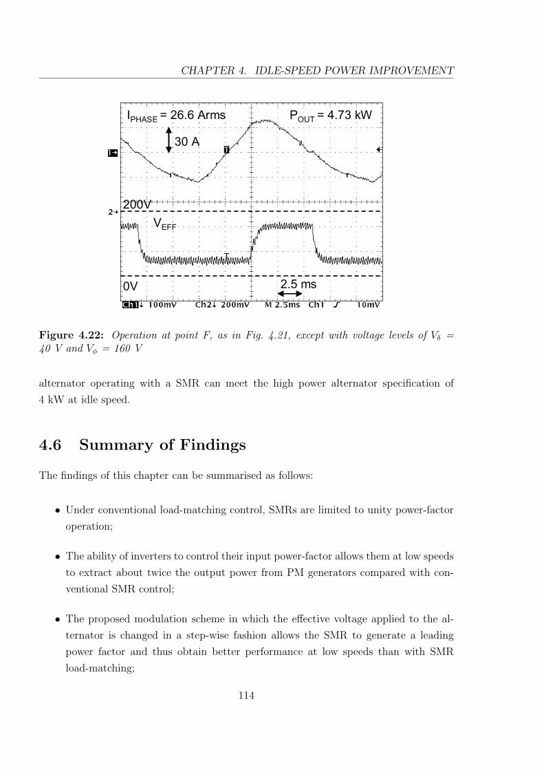
CHAPTER 4. IDLE-SPEED POWER IMPROVEMENT
IPHASE = 26.6 Arms
30 A
VEFF
200V
2.5 ms
POUT = 4.73 kW
0V
IPHASE = 26.6 Arms
30 A
VEFF
200V
2.5 ms
POUT = 4.73 kW
0V
Figure 4.22: Operation at point F, as in Fig. 4.21, except with voltage levels of Vδ =40 V and Vφ = 160 V
alternator operating with a SMR can meet the high power alternator specification of
4 kW at idle speed.
4.6 Summary of Findings
The findings of this chapter can be summarised as follows:
• Under conventional load-matching control, SMRs are limited to unity power-factor
operation;
• The ability of inverters to control their input power-factor allows them at low speeds
to extract about twice the output power from PM generators compared with con-
ventional SMR control;
• The proposed modulation scheme in which the effective voltage applied to the al-
ternator is changed in a step-wise fashion allows the SMR to generate a leading
power factor and thus obtain better performance at low speeds than with SMR
load-matching;
114
CHAPTER 4. IDLE-SPEED POWER IMPROVEMENT
• Careful selection of the modulation control parameters is required to optimize the
output power performance without exceeding rated current;
• Simulation results predicted that the calculated output power with a SMR at the
alternator idle speed of 1,800 rpm can be increased from 3.5 kW with conventional
SMR control, to 5.7 kW with the proposed control scheme, in comparison to the
calculated value of 6.5 kW with an inverter; and
• Experimental results showed a measured output power increase from 2.84 kW with
conventional SMR control to 4.73 kW with the proposed control scheme, which
meets the 4 kW high power alternator specification
This section has demonstrated that the proposed modulation scheme can produce
substantial low-speed output power improvements with the interior PM alternator studied.
Future work may include a more extensive examination of experimental results at various
operating points and further investigation to better understand the discrepancies between
the calculated and measured current waveforms.
115
Chapter 5
Conclusions
5.1 Background
The next generation of consumer vehicles is slated to include new features to enhance
performance, safety and comfort. Some examples of these features include active electro-
magnetic suspension to smooth out bumps and jolts, or electromechanical engine valve
timing to run the engine efficiently at all speeds. These emerging features, together with
the electrification of traditionally mechanically-driven accessories, come at the cost of
greater electrical power consumption, so it must be ensured that the alternator acting as
the power supply of a car is also prepared for the next generation.
The electrical power demand in cars has risen steadily from around 1 kW in 1985 to
almost 2.5 kW in 2005 and continues to grow [6, 8]. The conventional Lundell alternator
presently used in vehicles typically achieves an output power of 1 to 2 kW and would
be hard-pressed to satisfy future power requirements, so there is clear motivation for the
development of higher power alternators is clear. Towards this effort, the MIT/Industry
Consortium on Advanced Automotive Electrical/Electronic Components and Systems [4]
has provided several recommendations. Briefly, a suitable high power alternator should
provide:
• More power - output power ranging from 4 kW at engine idle speed (600 rpm) to
6 kW at top speed (6,000 rpm), corresponding approximately to a constant power
speed range of 10:1
• Better efficiency - requirement of 75% efficiency at 75% load at 1,500 rpm
116
CHAPTER 5. CONCLUSIONS
• Higher and steadier output voltage - maintain strict voltage limits around a 42 V
output voltage as specified by the 42V Powernet specification
Ideally, an alternator should also be inexpensive, robust and require minimal mainte-
nance.
Most significant of the Consortium’s recommendations is the move from the present
14 V electrical rail to a 42 V system. The higher system voltage allows the use of a lower
current to deliver the necessary power to car loads, resulting in a nine-fold reduction
in copper losses alone. This improved efficiency is especially important at higher power
levels. The higher system voltage also necessitates stricter voltage regulation to ensure
safety and this has been formalised in the SAE/MIT 42V Powernet standard [6].
Practical high power alternator solutions are currently being pursued, with efforts
involving electrical machines of various types, e.g. induction machines, permanent magnet
(PM) machines and reluctance machines. The greatest challenge in many cases has been
to maintain the required output power across the wide operating speed range. A second
key concern is the power electronics used to rectify and regulate the output power, as the
cost of power electronics is one of the most significant factors in determining the cost of
the alternator system as a whole.
5.2 Original Contributions
This thesis has investigated the power generation and control characteristics of a concept-
demonstrator interior PM alternator intended to satisfy the recommendations for a high
power alternator. The alternator was based on a 6 kW interior PM machine specifically
designed for optimal field-weakening performance and therefore a very wide CPSR. The
machine also has a high back-EMF and high inductance, allowing it to act as a controllable
current source when operating in conjunction with a SMR.
In this interior PM machine application, the SMR was used to provide voltage rectifi-
cation and regulation of voltage transients, to perform load-matching to maximise power
transfer to alternator loads and to increase the output power obtained at low speeds. The
SMR is a much cheaper alternative to an inverter while still allowing more flexibility of
control and greater output power than the bridge rectifier used in conventional Lundell
alternators.
The original contributions of this work in investigating the generation and control
characteristics of the interior PM alternator and SMR are summarised below:
117

CHAPTER 5. CONCLUSIONS
• Introduction of the VI locus as a tool in the steady-state modelling of electrical
machines.
• Development of steady-state and dynamic models to analyse the performance of the
interior PM machine operating in UCG, capable of predicting the effects of saliency,
magnetic saturation and stator resistance on generation and in particular hysteresis
in the output current. Experimental validation of the model predictions.
• Experimental demonstration of hysteresis in interior PM machines, which has not
previously been demonstrated, in accordance with model predictions.
• Investigation and modelling of SMR-based control of the interior PM machine out-
put. Experimental demonstration of alternator output power maximisation through
load-matching and closed-loop voltage regulation and transient suppression using
the SMR.
• Dynamic modelling of a phase-advance modulation scheme to improve the output
power of the interior PM alternator at idle speed. Implementation of the phase-
advance modulation scheme on a microcontroller, obtaining a measured increase in
idle-speed output power of 67%.
These contributions and other findings are further elaborated in the following subsec-
tions.
5.3 Interior PM Machine Generation Characteristics
In order to utilise the specially-designed interior PM machine [16] as an alternator, its
operating characteristics were theoretically and experimentally investigated. In particu-
lar, the case of interior PM generation into a DC voltage source load, also known as UCG
was studied as this is analogous to a car alternator charging a battery. The effects of
various parameters such as stator resistance, saliency and magnetic saturation on its gen-
eration characteristics were examined, as well as the interesting phenomenon of hysteresis
occurring in the stator current versus speed characteristic.
Voltage-Current Loci
• The concept of the VI locus of an interior PM machine was introduced as an an-
alytical tool, which to the author’s knowledge has not previously been applied
118

CHAPTER 5. CONCLUSIONS
to interior PM machines. VI loci are a visualisation of the relationship between
the steady-state output voltage and stator current of a PM machine while gen-
erating into a three-phase resistive load. They have been used throughout this
thesis to illustrate the generating behaviour of the interior PM machine under
various conditions.
Effect of Machine Parameters on Generation
• A steady-state d-q model of the interior PM machine was used to produce cal-
culated VI loci in order to investigate the effects of various parameters such as
saliency, stator resistance and magnetic saturation on the output current of two
interior PM machines. These predictions were validated against experimental
results including measurements of hysteresis, which have not previously been
demonstrated.
• Voltage overshoot and hence hysteresis only occurs for machines with a saliency
ratio of greater than two. Neglecting non-ideal effects, the size of the voltage
overshoot is proportional to the machine saliency and independent of speed.
• The presence of magnetic saturation and stator resistance both act to reduce
voltage overshoot. Additionally, the effect of resistance is more pronounced
at low speeds where the machine reactances are comparatively small and the
resistance therefore dominates the machine impedance.
Equivalent Circuit Models
• The validity of three equivalent circuit models of UCG were evaluated by com-
paring calculated curves against experimental results obtained using each of
the configurations. The VI loci experimentally measured from a rectifier and
resistive load accurately predicted the stator current versus speed characteristic
measured with a rectifier and DC voltage source load, therefore the modelling
of a DC voltage source load as a resistive load can be considered valid.
• The modelling of a rectifier and resistive load by a three-phase resistive load
was found to be not entirely valid, producing an overestimation of voltage
overshoot in the VI loci. It follows that this inaccuracy likewise affects the
predictions for a rectifier and voltage source load (UCG). It is possible that
the action of the rectifier causes currents in the portion of the locus which is
typically close to the threshold of generation to become highly discontinuous,
119

CHAPTER 5. CONCLUSIONS
thereby violating the assumption of sinusoidal current waveforms upon which
the steady-state model is based.
• The dynamic model used was shown to accurately predict the shape of the
current and voltage waveforms of the interior PM machine during UCG, even
under highly discontinuous currents. This causes it to be more accurate than
the steady-state model in predicting the waveforms near the threshold of gener-
ation and therefore the amount of hysteresis that may be observed in a machine.
Stator Current Hysteresis
• VI loci were used to explain the phenomenon of hysteresis in the UCG stator
current versus speed characteristic. Hysteresis was shown to arise from ’voltage
overshoot’, which is a characteristic observable in the VI locus of a machine
whereby the machine is capable of producing an output voltage under load
which is greater than the open-circuit voltage.
• Stator current hysteresis has not had an impact on the generation performance
of the interior PM machine used in this study because the desired operating
DC link voltage was too low for hysteresis to manifest. The methods used in
this study can be applied to predict the presence and extent of hysteresis in
other cases where it may be an issue in the control of an interior PM alternator.
5.4 Switched-Mode Rectifier Control
Whereas the output of a conventional Lundell alternator is controlled by adjusting
the field current, the output of the interior PM alternator is controlled by the SMR. The
SMR provides the functions of voltage regulation and transient suppression and is thus
the means by which the alternator can satisfy the voltage requirements outlined in the
42V Powernet specification.
Both the steady-state and dynamic characteristics of the alternator and SMR system
were theoretically and experimentally investigated, first as an open-loop system and later
as a closed-loop system after a suitable closed-loop controller had been designed and
implemented.
In all tests involving the SMR, the interior PM alternator was fitted with a 135 V
stator in order to accommodate the available SMR unit rated for 200 V, 50 A. The DC
120
CHAPTER 5. CONCLUSIONS
link voltage was set at 200 V and thus for a desired output power of 6 kW, the alternator
DC output current was 35 A. To achieve a true 42 V system in accordance with the 42V
Powernet specification, the alternator would need to be fitted with a lower voltage stator,
however the SMR would then need to be rated for at least 150 A. The results obtained
in these tests can nevertheless be considered indicative of the alternator’s performance.
Alternator SMR Duty-Cycle Response
• Control of the SMR was achieved by adjusting the duty-cycle of PWM signals
fed to the gates of the SMR switches. Varying the duty-cycle has different
effects depending on the operating speed of the alternator:
• At low speeds where the open-circuit back-EMF of the alternator is insufficient
to overcome the DC link voltage, the SMR acts similarly to a boost converter
- instead of being exposed to the full DC link voltage VDC , the alternator
sees a reduced effective voltage VEFF = (1 − d)VDC , determined by the SMR
duty-cycle d. For a fixed DC link voltage such as a car battery, this lowers
the minimum operating speed at which the alternator starts to generate cur-
rent. The appropriate adjustment of the duty-cycle to match the alternator to
the load in this manner resulted in a smooth increase in output power from
standstill up to approximately 3,000 rpm, above which no boosting action is
necessary (see Fig. 3.21).
• At high speeds, changing the effective voltage has little effect on the alternator
output current and the alternator provides a nearly constant current IIN to the
SMR. Varying the duty-cycle controls the portion of current IOUT = (1−d)IIN
which is delivered to the load. This is a key point in the control of the interior
PM alternator and was supported by the relatively constant predicted input
current vs. duty-cycle (IIN vs. d) characteristic. These relationships were
experimentally verified and it was found that the non-linear region around the
threshold of generation appeared at higher than predicted values of duty-cycle
and thus the current versus duty-cycle relationship was less linear than ex-
pected (see Fig. 3.17). This resulted in the measured alternator currents being
lower than predicted by a few amps. These discrepancies can be attributed to
the previously mentioned inaccuracy of the steady-state model when handling
non-sinusoidal waveforms.
Power and Efficiency
121

CHAPTER 5. CONCLUSIONS
• The power requirements for a high power alternator correspond to 4 kW at
engine idle speed (1,800 rpm) and 6 kW at top speed (18,000 rpm). Since
the dynamometer rig used to take experimental measurements was limited to
6,000 rpm, it was not possible to measure the top-speed result, however, the
output power obtained at 6,000 rpm was 6.6 kW. Given the design of the inte-
rior PM alternator for optimum field-weakening performance, it is reasonable
to expect that the high-speed requirement is achievable (see Fig. 3.21).
• The predicted alternator output power at idle speed was 3.5 kW, which does
not satisfy the idle-speed power requirement of 4 kW. The actual measured
power was 18% lower, at 2.84 kW. This is also reflected in the lower than
expected output current of 14.7 A as compared with a predicted 17.5 A.
• The efficiency requirement from the 42V specification was 75% efficiency at
75% load at an engine speed of 1,500 rpm. This corresponds to a load of
4 kW at an alternator speed of 4,500 rpm. The efficiency of the interior PM
alternator at this point is 71%.
Closed-Loop Control
• The transient current response of the alternator and SMR system was experi-
mentally determined by injecting sinusoidally-varying SMR control signals and
the resulting response was modelled by a second-order transfer function. A sim-
ple closed-loop controller with proportional gain was designed and implemented
based on the modelled system function.
• The closed-loop controller was successful in regulating the output voltage to
200 V DC while the alternator was operating at 1,500 rpm. Measurements
showed a 1% decrease in average output voltage for a 25% increase in load
current, i.e. a ± 2% variation in average output voltage over the entire load
range. Some steady-state output voltage oscillations were present under higher
current loads. These oscillations were limited to within the 190 V to 210 V
range, i.e ± 10% output voltage. The nominal operating voltage from the 42V
Powernet specification is 42 V, with an allowable steady-state variation from
30 V to 50 V. This is roughly equivalent to a range of ± 19% nominal voltage,
which the controller easily satisfies.
• The ability of the controller and SMR to suppress transient overvoltages was
successfully demonstrated through load dump tests. The maximum overvoltage
122

CHAPTER 5. CONCLUSIONS
produced by the closed-loop system in response to a load current step of 8.8 A
(representing an 880 W load dump) was 10 V. The load dump transient reached
a peak value of 110% nominal output voltage and settled to steady-state value
within 20 ms. As a comparison, the 42V specification of 58 V is equivalent to
138% nominal voltage.
Output Power Improvement
• The output power achieved by the interior PM alternator operating with the
SMR at idle speed (1,800 rpm) was 2.8 kW, which does not satisfy the high
power alternator requirement of 4 kW. In order to address this issue of in-
sufficient idle-speed power, a SMR modulation scheme employed by Rivas,
Perreault and Keim to improve output power in a Lundell alternator was ex-
amined [15]. This modulation scheme has previously been shown to improve
idle-speed power output by up to 15%.
• To better understand the limitations of the SMR, the operating trajectories
of the alternator under both SMR load-matching and inverter operation were
examined using analytical models. The ability of inverters to generate a leading
input power-factor allows them to extract twice the output power at low speeds
as compared with SMR load-matching. By applying a varying effective DC link
voltage to each phase over the electrical period of the alternator, the proposed
SMR modulation scheme allows the current waveform to be shaped. This can
be used to generate a certain degree of leading phase shift in the fundamental
of the modulated waveform.
• A Simulink model was constructed to predict the performance of the scheme as
applied to the interior PM alternator. Simulations showed that at idle speed
and rated current it would be able to offer performance lying between that of
SMR load-matching and inverter operation, providing an approximately 70%
increase in output power over SMR load-matching performance.
• The modulation scheme was implemented on a dsPIC microcontroller. The
controller was programmed to allow the modulation parameters to be adjusted
in real time during alternator operation. Experimental tests conducted over
a range of modulation parameter values showed a 67% increase in idle-speed
output power from 2.84 kW with SMR load-matching to 4.73 kW with the
123

CHAPTER 5. CONCLUSIONS
SMR modulation scheme, thereby satisfying the idle-speed power requirement
of 4 kW.
5.5 Summary
The aim of this study was to examine the operation of an interior PM machine with a
switched-mode rectifier as a high power alternator.
The implementation of basic closed-loop voltage regulation as well as a SMR modu-
lation technique to improve low-speed output power have demonstrated that the concept
demonstrator interior PM alternator is capable of satisfying the voltage and low-speed
power requirements of the SAE/MIT 42V specification using inexpensive power electronics
and simple control.
Additionally, in examining the interior PM machine generation characteristics, steady-
state and dynamic models have been developed to investigate the effect of various parame-
ters such as saliency, stator resistance, magnetic saturation, DC link voltage and operating
speed on the generating performance of the alternator. These provide a framework for
understanding and predicting alternator performance.
The performance of the interior PM alternator against the high power alternator
specifications are summarised as follows:
• The alternator achieved an output power of 4.73 kW at 1,800 rpm and 6.8 kW
at 6,000 rpm which satisfies, over the tested speed range, the specified 4 kW at
1,800 rpm and 6 kW at 18,000 rpm (see Fig. 5.1)
• The efficiency measured at 1,500 rpm under 75% load was 71%, which does not
satisfy the specified efficiency of 75%
• The measured steady-state output voltage variation was ± 10% nominal voltage,
satisfying the specification of ± 19% nominal voltage
• The maximum transient voltage peak measured under load dump conditions was
110% nominal voltage, satisfying the specification of 138% nominal voltage
The wide constant-power speed range of the interior PM alternator in this study also
makes it suitable for renewable energy applications. The SMR provides a useful degree
of control in order to dynamically optimise the power transfer to a battery, particularly
in wind turbines where the rotational speed of the alternator due to the wind may vary
widely.
124

CHAPTER 5. CONCLUSIONS
0 1.8 180
2
4
6
8
Speed [krpm]
Out
put P
ower
[kW
]
inverter (calculated)
specification
SMR load−matching (calculated) − 3.5 kW at idleSMR load−matching (measured) − 2.8 kW at idle
SMR with power improvement (measured) − 4.73 kW at idle
Figure 5.1: Output power versus speed characteristics for the interior PM alternatorcompared against high power alternator power specifications
5.5.1 Further Work
Although this project has investigated the operation of a interior PM alternator and
demonstrated that it is capable of satisfying some of the requirements of a high power
automotive alternator, there is still much scope for work and several areas could benefit
from further attention:
• Experimental tests at higher alternator speeds from 6,000 rpm to 18,000 rpm have
not been conducted due to the limitations of the dynamometer rig. Although it can
be expected that the good field-weakening performance of the interior PM machine
should allow it to maintain output power throughout the speed range, this should
be experimentally verified. Due to the presence of magnet cavities, the structural
strength of the interior PM rotor may need to be assessed for high speed tests.
• The accuracy of the steady-state interior PM machine model appears to be affected
by the presence of a rectifier. This inaccuracy has been observed as an overestima-
tion of voltage overshoot in the predicted steady-state VI loci. This may be due to
the presence of non-sinusoidal current and voltage waveforms caused by a rectifier.
Whilst the steady-state model is limited by its assumption of sinusoidal waveforms,
preliminary dynamic model simulations without this limitation have also predicted
similar results.
• The inconsistency found between the dynamic response observed in the duty-cycle
step response of the alternator and the Bode plot measurements suggest that the
125

CHAPTER 5. CONCLUSIONS
accuracy of the modelled transfer function may need to be improved. Inaccurate
modelling of the transfer function may be the cause of the steady-state oscillations
observed in the closed-loop system. Other possible causes are non-linearity in the
output current response, mechanical oscillations in the dynamometer rig, or digi-
tal control loop limitations. It is possible that the greater mechanical stiffness of
an automotive engine as compared with the dynamometer rig may alleviate this
problem.
• A more sophisticated controller may provide better performance with respect to
reducing steady-state oscillations. Designs involving integral and differential gain
were considered, however no significant improvement was predicted by simulations.
Other options such as a feed-forward mechanism may also be applied, however
further designs were not implemented as it was decided that improving the idle-
speed output power was more important in meeting alternator specifications.
• The most severe load dump test conducted involved a dump of 800 W. Although the
controller responded quickly in this case to clamp the voltage to 110% nominal volt-
age, more severe load dump tests should be carried out. These were not attempted
in this study due to concerns with the mechanical robustness of the dynamometer
rig under such stresses.
• The controller could be modified to incorporate both closed-loop voltage regulation
and the idle-speed power improvement modulation scheme. The location of optimum
operating points in the modulation parameter space at speeds other than idle has
not been investigated and this knowledge would be essential for such a variable-
speed controller. The modulation scheme also offers the possibility of obtaining
comparable output power to conventional load-matching but with a reduced stator
current and therefore losses. This adds extra power management flexibility to the
controller.
• The iron losses in the interior PM alternator rise significantly with speed. This
is likely due to the high frequency flux density harmonics under field-weakening
operation. Modification of the rotor design to reduce this effect could improve the
efficiency of the alternator and aid in achieving the efficiency specification [41].
126
Bibliography
[1] A. Emadi, Handbook of Automotive Power Electronics and Drives. CRC Press, 2005.
[2] J. Miller, “Multiple Voltage Electrical Power distribution System for Automotive Ap-
plications,” in 31st Intersociety Energy Conversion Engineering Conference, Wash-
ington, D.C, August 1996.
[3] Forum Bordnetz, “Year 2005 generic luxury vehicle,” 2000, homepage bordnetzforum-
42V.de.
[4] E. Lovelace, “Optimization of a Magnetically Saturable Interior Permanent-Magnet
Synchronous Machine Drive,” Ph.D. dissertation, Massachusetts Institute of Tech-
nology, June 2000.
[5] J. Kassakian and D. Perreault, ““The Future of Electronics in Automobiles“,” in
Power Semiconductor Devices and ICs, Proceedings of the 13th International Sym-
posium on, 2001, pp. 15–19.
[6] P. Nicastri and H. Huang, “42V PowerNet: Providing the Vehicle Electrical Power
for the 21st Century,” SAE Transactions, vol. 109, no. 7, pp. 447–453, 2000.
[7] G. Hassan, D. Perreault, and T. Keim, “Design of dual-output alternators with
switched-mode rectification,” IEEE Transactions on Industry Applications, vol. 20,
no. 1, pp. 164–172, 2005.
[8] J. Kassakian, “Automotive electrical systems-the power electronics market of the
future,” in Proceedings of the IEEE Applied Power Electronics Conference, vol. 1,
Feb. 2000, pp. 3–9.
[9] D. Perreault and V. Caliskan, “Automotive Power Generation and Control,” IEEE
Transactions on Power Electronics, vol. 19, no. 3, pp. 618–630, 2004.
127

BIBLIOGRAPHY
[10] M. Naidu and J. Walters, “A 4-kW 42-V Induction-Machine-Based Automotive
Power Generation System With a Diode Bridge Rectifier and a PWM Inverter,”
IEEE Transactions on Industry Applications, vol. 39, no. 5, pp. 1287–1293, 2003.
[11] R. Henry, B. Lequesne, J. Ronning, and Y. Xue, “Belt-Driven Starter-Generator for
Future 42-Volt Systems,” Technical Paper, Society of Automotive Engineers, March
2001.
[12] B. Lequesne, R. Henry, Y. Xue, and J. Ronning, “Design and Testing of a Belt-Driven
Induction Starter-Generator,” IEEE Transactions on Industry Applications, vol. 38,
no. 6, pp. 1525–1533, 2002.
[13] J. Miller, A. Gale, P. McCleer, F. Leonardi, and J. Lang, “Starter-Alternator for Hy-
brid Electric Vehicle: Comparison of Induction and Variable Reluctance Machines
and Drives,” in Proceedings of the IEEE Industry Applications Society Annual Meet-
ing, 1998, pp. 513–523.
[14] R. Schiferl and T. Lipo, “Power Capability of Salient Pole Permanent Magnet Syn-
chronous Motor in Variable Speed Drive Applications,” IEEE Transactions on In-
dustry Applications, vol. IA-23, pp. 115–123, 1990.
[15] J. Rivas, D. Perreault, and T. Keim, “Performance Improvement of Alternators with
Switched-Mode Rectifiers,” IEEE Transactions on Energy Conversion, vol. 19, no. 3,
pp. 561–568, 2004.
[16] W. Soong and N. Ertugrul, “Inverterless High Power Interior Permanent Magnet
Automotive Alternator,” IEEE Transactions on Industry Applications, vol. 19, no. 4,
pp. 1083–1091, 2004.
[17] M. Allen, “Whatever Happened to the 42-Volt Car?” http://www.popularmechanics.
com/cars/news/4226979, 2009, [Online; accessed 15-July-2011].
[18] A. Emadi, Y. J. Lee, and K. Rajashekara, “Power electronics and motor drives in
electric, hybrid electric, and plug-in hybrid electric vehicles,” IEEE Transactions on
Industrial Electronics, vol. 55, no. 6, pp. 2237 –2245, June 2008.
[19] S. Deffree, “Gearing up to 42V,” Electronic News, Nov. 2002.
[20] G. Wagner and S. Irving, “Gear up for the shift to 42V systems,” EETimes Asia,
Apr. 2007.
128
BIBLIOGRAPHY
[21] M. Shrud, A. Bousbaine, A. Elazrag, and N. Benamrouche, “Analysis and simulation
of a 42v power system for automotive applications,” in Universities Power Engineer-
ing Conference (UPEC), 2009 Proceedings of the 44th International, Sept. 2009, pp.
1 –5.
[22] D. Stoia and M. Cernat, “Design of a 42 v automotive alternator with integrated
switched-mode rectifier,” in Advanced Electromechanical Motion Systems Electric
Drives Joint Symposium, 2009. ELECTROMOTION 2009. 8th International Sym-
posium on, July 2009, pp. 1 –8.
[23] C. Mudannayake and M. Rahman, “Control design of an induction machine based
integrated starter alternator for 42v powernet,” in Industry Applications Conference,
2006. 41st IAS Annual Meeting. Conference Record of the 2006 IEEE, vol. 3, Oct.
2006, pp. 1585 –1592.
[24] Z. Xueyi, Z. Qingliang, and S. Liwei, “Study on controlled rectification constant-
voltage of the 42v rare-earth permanent-magnet generator on vehicles,” in Computer,
Mechatronics, Control and Electronic Engineering (CMCE), 2010 International Con-
ference on, vol. 4, Aug. 2010, pp. 24 –27.
[25] D. Xiao, K. You, and M. Rahman, “Implementation of a matrix-z-source converter
for isa 42v system using indirect space vector modulation,” in Electrical Machines
and Systems (ICEMS), 2011 International Conference on, Aug. 2011, pp. 1 –6.
[26] S. C. Tang, D. Otten, T. Keim, and D. Perreault, “Design and evaluation of a 42-v
automotive alternator with integrated switched-mode rectifier,” IEEE Transactions
on Energy Conversion, vol. 25, no. 4, pp. 983 –992, Dec. 2010.
[27] F. Carrichi, F. Crescimbini, E. Santini, and L. Solero, “High-Efficiency Low-Volume,
Starter/Alternator for Automotive Applications,” in Proceedings of the IEEE Indus-
try Applications Society Annual Meeting, vol. 1, 2000, pp. 215–222.
[28] F. Liang, J. Miller, and S. Zarei, “A Control Scheme to Maximize Output Power
of a Synchronous Alternator in a Vehicle Electrical Power Generation System,” in
Proceedings of the IEEE Industry Applications Society Annual Meeting, vol. 2, 1996,
pp. 830–835.
129

BIBLIOGRAPHY
[29] E. Lovelace, T. Jahns, and J. Lang, “Impact of saturation and inverter cost on in-
terior pm synchronous machine drive optimization,” IEEE Transactions on Industry
Applications, vol. 36, no. 3, pp. 723–729, 2000.
[30] M. Naidu, R. Henry, and N. Boules, “A 3.4 kW, 42 V High Efficiency Automotive
Power Generation System,” Technical Paper, Society of Automotive Engineers.
[31] D. Whaley, G. Ertasgin, W. Soong, N. Ertugrul, J. Darbyshire, H. Dehbonei, and
C. Nayar, “Investigation of a low-cost grid-connected inverter for small-scale wind
turbines based on a constant-current source PM generator,” 32nd Annual Conference
on Industrial Electronics, pp. 4297–4302, 2006.
[32] M. Pathmanathan, W. Soong, and N. Ertugrul, “Output power capability of surface
PM generators with switched-mode rectifiers,” Proceedings of the IEEE International
Conference on Sustainable Energy Technologies, pp. 1–6, 2010.
[33] M. Pathmanathan and W.L. Soong and N. Ertugrul, “Investigation of phase advance
modulation with surface permanent magnet generators,” in Power Engineering Con-
ference, 2009. AUPEC 2009. Australasian Universities, Sept. 2009, pp. 1 –6.
[34] M. Pathmanathan, W. Soong, and N. Ertugrul, “Maximum torque per ampere con-
trol of phase advance modulation of a spm wind generator,” in Energy Conversion
Congress and Exposition (ECCE), 2011 IEEE, Sept. 2011, pp. 1676 –1683.
[35] A. Adnanes, “Power Feed-Back During Controller Failure in Inverter Fed Perma-
nent Magnet Synchronous Motor Drives with Flux-Weakening,” in Proceedings of
the IEEE Power Electronics Specialists, 1992, pp. 958–963.
[36] V. Caliskan, D. Perreault, T. Jahns, and J. Kassakian, “Analysis of Three-Phase Rec-
tifiers with Constant-Voltage Loads,” IEEE Transactions on Circuits and Systems—
Part I: Fundamental Theory and Applications, vol. 50, no. 9, pp. 1220–1225, 2003.
[37] T. Jahns and V. Caliskan, “Uncontrolled Generator Operation of Interior PM Syn-
chronous Machines Following High-Speed Inverter Shutdown,” IEEE Transactions
on Industry Applications, vol. 35, no. 6, pp. 1347–1357, 1999.
[38] B. Welchko, T. Jahns, W. Soong, and J. Nagashima, “IPM Synchronous Machine
Drive Response to Symmetrical and Asymmetrical Short Circuit Faults,” IEEE
Transactions on Energy Conversion, vol. 18, no. 2, pp. 291–298, 2003.
130

BIBLIOGRAPHY
[39] W. Soong and N. Ertugrul, “Field-Weakening Performance of Interior Permanent
Magnet Motors,” IEEE Transactions on Industry Applications, vol. 38, no. 5, pp.
1251–1258, 2002.
[40] J. Kikuchi, M. Manjrekar, and T. Lipo, “Performance Improvement of Half Con-
trolled Three Phase PWM Boost Rectifier,” in Proceedings of the IEEE Power Elec-
tronics Specialists, 1999, pp. 319–324.
[41] V. Zivotic-Kukolj, W. Soong, and N. Ertugrul, “Investigation of Iron Losses in a
High Flux Interior PM Automotive Alternator,” in Proceedings of Australasian Uni-
versities Power Engineering Conference (AUPEC), vol. 3, 2004.
131

Appendix A
Publications
1. C. Liaw, W. Soong, B. Welchko and N. Ertugrul, ”Uncontrolled Generation in In-
terior Permanent Magnet Machines,” IEEE Transactions on Industry Applications,
vol. 41, no. 4, pp. 945–954, 2005.
2. C. Liaw, D. Whaley, W. Soong and N. Ertugrul, ”Investigation of Inverterless Con-
trol of Interior Permanent Magnet Alternators,” IEEE Transactions on Industry
Applications, vol. 42, no. 2, pp. 536–544, 2006.
3. C. Liaw, W. Soong and N. Ertugrul, ”Closed-Loop Control and Performance of an
Inverterless Interior PM Automotive Alternator,” in Proceedings of the International
Conference on Power Electronics and Drive Systems, vol. 1, pp. 343–348, 2005.
4. C. Liaw, W. Soong and N. Ertugrul, ”Low-Speed Output Power Improvement of an
Interior PM Automotive Alternator,” in Proceedings of the IEEE Industry Applica-
tions Society Annual Meeting, vol. 1, pp. 27–34, 2006.
132

C. Liaw, W. Soong, B. Welchko and N. Ertugrul (2005) Uncontrolled Generation in
Interior Permanent Magnet Machines.
IEEE Transactions on Industry Applications, v. 41, (4), pp. 945-954, July/August
2005
NOTE: This publication is included in the print copy of the thesis
held in the University of Adelaide Library.
It is also available online to authorised users at:
http://dx.doi.org/10.1109/TIA.2005.851557

C. Liaw, D. Whaley, W. Soong and N. Ertugrul (2006) Investigation of Inverterless
Control of Interior Permanent Magnet Alternators.
IEEE Transactions on Industry Applications, v. 42, (2), pp. 536-544, March/April
2006
NOTE: This publication is included in the print copy of the thesis
held in the University of Adelaide Library.
It is also available online to authorised users at:
http://dx.doi.org/10.1109/TIA.2005.863910

C. Liaw, W. Soong and N. Ertugrul (2005) Closed-Loop Control and Performance of
an Inverterless Interior PM Automotive Alternator.
Proceedings of the International Conference on Power Electronics and Drive
Systems, 2005. PEDS 2005, v. 1, pp. 343-348
NOTE: This publication is included in the print copy of the thesis
held in the University of Adelaide Library.
It is also available online to authorised users at:
http://dx.doi.org/10.1109/PEDS.2005.1619710

C. Liaw, W. Soong and N. Ertugrul (2006) Low-Speed Output Power Improvement of
an Interior PM Automotive Alternator.
Proceedings of the IEEE Industry Applications Society Annual Meeting, 41st IAS
Annual Meeting, v. 1, pp. 27-34, October 2006
NOTE: This publication is included in the print copy of the thesis
held in the University of Adelaide Library.
It is also available online to authorised users at:
http://dx.doi.org/10.1109/IAS.2006.256516

Appendix B
Programs
This appendix contains code listings of the main programs used in the course of this work
both to produce theoretical simulations of the interior PM alternator and to control the
alternator power electronics.
B.1 Matlab and Simulink Code
Listing B.1: Steady-state model calculation of interior PM machine voltage-current loci
% Generate normal i sed VI l o c i vs speed/ r e s i s t a n c e / s a l i e n c y / sa tu ra t i on
% ( us ing sa tu ra t i on model de s c r ibed by Jahns )
c l e a r
v rated = 69 . 3 ;
i r a t e d = 2 . 8 3 ;
r r a t ed = v rated / i r a t e d ;
% Stator Parameters
Rph = 0 ; %2.94; % phase r e s i s t a n c e for 1500 rpm case
Eo= 69.3/ sq r t ( 3 ) ; % machine open−c i r c u i t back−emf , Vrms per phase at Wrpm Eo
% from Rotor 3 Test 3 data
po l e s = 2 ; % number o f po le pa i r s
phases =3 ; % number o f phases
% 2 .2kW Rotor 4b with NdFeB s o l i d magnets
Wrpm Eo = 1500 ; % speed in rpm at which Eo i s de f ined
W Eo = Wrpm Eo ./ 60 .∗ 2 .∗ pi .∗ po l e s ;
Psi = Eo ./ W Eo; % ca l c u l a t e f l ux l i nkage (Vrms/ rad/ s )
% de f i n e va lues o f Ld and Lq
L dn = 0 . 0 45 ; % d−ax i s phase inductance
L qno = 0 . 3 45 ; % q−ax i s phase inductance unsaturated
L qn = 0 . 3 45 ; % q−ax i s phase inductance s t a r t i n g value
for Rph = 6.0 % [ 0 : 0 . 2 : 0 . 8 1 .2 1 .8 3 . 0 ] . ∗ r r a t ed % [ 0 : 0 . 1 : 8 . 0 ] ,
% Normalised R c a l c u l a t i o n s
Wtest = 1500;
w= 2∗ pi ∗(Wtest /60)∗ po l e s ;
R n = Rph/(w∗L dn )
166

APPENDIX B. PROGRAMS
Rph unity = 1∗(w∗L dn )
for Xi = 6% [1 2 4 6 8];% 32 64 128 25 512 1024 2048 ] ,
L qno = L dn∗Xi ;
L qn = L qno ;
for beta n = 0 %[0 1 2 3 6 16]%40 80 100 200 ] ,
for Wtest= [ 1 : 5 ]∗ 1 5 0 0 . / 5 , %[110 225 450 700 1000 1500 ]
%%%%%%%%%%%%%%%%%%%%%%%%%%%%%%%%%%%%%%%%%%%%%%%%%%%%%%%%%%%%%%%%%%%%%%%%%%%%%%%%
w= 2∗ pi ∗(Wtest /60)∗ po l e s ; % c a l c u l a t e maximum e l e c t r i c a l f requency
% R= logspace ( 0 , 3 , 3 00 ) ; % generate array o f r e s i s t a n c e s
R= logspace (−1 ,4 ,300) ; % generate array o f r e s i s t a n c e s
w rpm= w .∗60 . / (2∗ pi ) . / po l e s ;
for count =1:10
theta= atan ( (R+Rph) . / (w .∗ L qn ) ) ; % f ind angle between cur rent and d−ax i s
Z= (R+Rph) .∗ s i n ( theta ) + w .∗ L dn .∗ cos ( theta ) ; % c a l c u l a t e load Z
I s a l i e n t = Psi .∗ w ./ Z ; % ca l c u l a t e phase cur rent
% ca l c u l a t e Id and Iq
I qn= I s a l i e n t .∗ s i n ( theta ) ;
I dn= I s a l i e n t .∗ cos ( theta ) ;
% f ind new value o f Lq based on Iq
Lq new= L dn + ( ( L qno − L dn ) . / sq r t (1 + ( beta n .∗ I qn ) . ˆ 2 ) ) ;
e r r o r= max(Lq new−L qn ) ;
L qn= Lq new ;
end
Tsa l i en t 18= po l e s .∗ phases .∗ ( Psi .∗ I qn + (L qn−L dn ) .∗ I dn .∗ I qn ) ;
Pmsal ient 18= Tsa l i en t 18 .∗ w / po l e s ;
Vsa l i en t 18= I s a l i e n t .∗ R;
Psa l i e n t 18= phases .∗ Vsa l i en t 18 .∗ I s a l i e n t ;
I s a l i e n t 1 8= I s a l i e n t ;
% Plot out r e s u l t s ( normal i sed vo l tage and current )
f i g u r e (1 )
p lo t ( sq r t ( 3 ) .∗ Vsa l i en t 18 . / v rated , abs ( I s a l i e n t 1 8 ) . / i r a t ed , ’k− ’ ) ;
hold on ;
% p lo t max vo l tage po int s
[ y , i ] = max( Vsa l i en t 18 ) ;
p l o t ( sq r t (3)∗y . / v rated , I s a l i e n t 1 8 ( i ) . / i r a t ed , ’ ro ’ ) ;
% % plo t s a l i e n c y va lues
% [ y , i ] = max( Vsa l i en t 18 ) ;
% text (y . /0 . 1986 + 0 .02 , I s a l i e n t 1 8 ( i ) , num2str (Xi ) ) ;
end
end
end
end
hold o f f ;
y l ab e l ( ’ Stator Current [ pu ] ’ )
x l ab e l ( ’ Line Voltage [ pu ] ’ )
ax i s ( [ 0 1 .4 0 1 . 1 ] ) ;
s e t (1 , ’ p o s i t i o n ’ , [ 524 324 860 4 0 0 ] ) ;
% t h e s i s f i g ( 1 ) ;
167

APPENDIX B. PROGRAMS
Simulink model used to calculate interior PM machine waveforms under uncontrolled
generation
Unc
ontr
olle
d ge
nera
tion
sim
ulat
ion
with
rec
tifie
r D
C o
utpu
t
set b
us v
olta
ge in
her
e
vpw
mtr
igge
r
vlin
elp
vlin
elp
wor
kspa
ce
vlin
elp
vlin
e
torq
ue
1500
spee
d rp
m
spee
d
(0)
shor
t to
grou
nd2
[0 0
0]
shor
t to
grou
nd1
[0 0
0]
shor
t to
grou
nd0
load
torq
ue
u[1]
-u[3
]
line
volta
ge
lam
_dqs
e
idqs
e
iabc
s
duty
duty
wor
kspa
ce
duty
cycl
e
Vab
c (P
h2bu
sG)
Tl (
Nm
)
wrm
lam
da_d
qse
(Wb)
idqs
e (A
)
Tor
que
(Nm
)
thet
a (r
ad)
iabc
s (A
)
Lq (
H)
dq m
odel
inte
rior
pmm
achi
ne
absI
f(u)
abs
iabc
s (A
)V
abc
(Ph2
busG
)
Unc
ontr
olle
dR
ectif
ier
1
0.00
1s+
1
Tra
nsfe
r F
cn
Sw
itch1
Sw
itch
Ste
p
Spe
ed
Spe
ed w
orks
pace
Sco
pe
Sat
urat
ion
Ram
p10
kHz
Ram
pQ
uant
izer
Lq
Idc1
Idc
wor
kspa
ce
Idc
[sw
]
[iabc
s]
-K-
Gai
n
[iabc
s]
[sw
]
[iabc
s]
0
Dut
y C
ycle
1-D
T[k
]
Dire
ct L
ook-
Up
Tab
le (
n-D
)
iabc
s (A
)Id
c
DC
Rec
tifie
r
168

APPENDIX B. PROGRAMS
Simulink model used to calculate dynamic response of interior PM machine under
closed-loop inverterless load-matching operation
Pd = 0.0002/(Ts)for optimum
Vout
z1
Unit Delay
Iload
To Workspace3
time
To Workspace2
vout
To Workspace1
duty
To Workspace
Saturation1 Saturation Sampling
Duty
Bus VoltageIOut
SMR
R
Resistive LoadProduct
95
Load1
0.1
Kp
0
Ki
0/(60e-6)
Kd
1s
Integrator
Duty
Tz-1
Discrete-TimeIntegrator
1/3000e-6
DC LinkCapacitance
Clock
1200^2s +1200*2s+1200^22
Alternator TF
ADC Quantizer
DC busvoltage
MirroredPhase Currents
1IOut
iout
To Workspace
Switch
SMR switching noise
Product
37.67/36
PeakValue
max
MinMax
MATLABFunction
MATLAB FcnIin_view
Ic1
Ic
Ib1
Ib
Ia1
Ia
1
Constant
2Bus Voltage
1Duty
SMR
169

APPENDIX B. PROGRAMS
Simulink model used to calculate interior PM machine waveforms under phase-advance
SMR modulation for idle-speed power improvement (main block)
set b
us v
olta
ge in
her
e
iabc
vlin
elp
wor
kspa
ce2
time
vlin
elp
wor
kspa
ce1
vlin
elp
vlin
elp
wor
kspa
ce
vlin
elp
vlin
e
torq
uepr
obe
torq
ue1
torq
ue w
orks
pace
1800
spee
d rp
m
spee
d
[0 0
0]
shor
t to
grou
nd0
load
torq
ue
u[1]
-u[3
]
line
volta
ge
lam
_dqs
e
idqs
e
iabc
s
Vab
c (P
h2bu
sG)
Tl (
Nm
)
wrm
lam
da_d
qse
(Wb)
idqs
e (A
)
Tor
que
(Nm
)
thet
a (r
ad)
iabc
s (A
)
Lq (
H)
dq m
odel
inte
rior
pmm
achi
ne
absI
f(u)
abs
1
0.00
1s+
1
Tra
nsfe
r F
cn
Out
1
Tim
e-va
ryin
gsp
eed
Spe
ed
Spe
ed w
orks
pace
Sco
peia
bcs
(A)
Vab
c (P
h2bu
sG)
SM
R
Lq
Idc1
Idc
wor
kspa
ce
Idc
spee
d
iabc
s
-K-
Gai
n
[iabc
s]
[iabc
s]
iabc
s (A
)Id
c
DC
Rec
tifie
r
Clo
ck
170
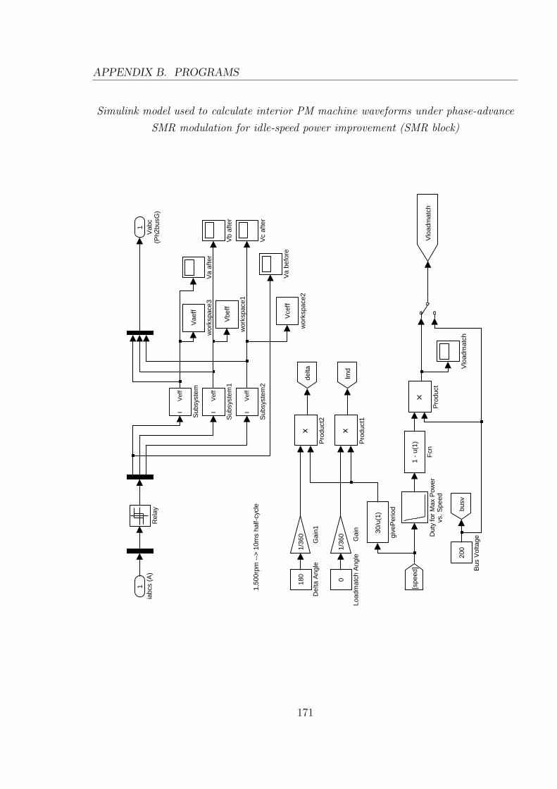
APPENDIX B. PROGRAMS
Simulink model used to calculate interior PM machine waveforms under phase-advance
SMR modulation for idle-speed power improvement (SMR block)
1,50
0rpm
-->
10m
s ha
lf-cy
cle
1V
abc
(Ph2
busG
)
Vae
ff
wor
kspa
ce3
Vce
ff
wor
kspa
ce2
Vbe
ff
wor
kspa
ce1
30/u
(1)
give
Per
iod
Vlo
adm
atch
Vc
afte
r
Vb
afte
r
Va
befo
re
Va
afte
r
IV
eff
Sub
syst
em2
IV
eff
Sub
syst
em1
IV
eff
Sub
syst
em
Rel
ay
Pro
duct
2
Pro
duct
1
Pro
duct
0
Load
mat
ch A
ngle
lmd
Vlo
adm
atch
busv
delta
1/36
0
Gai
n1
1/36
0
Gai
n
[spe
ed]
1 -
u(1)
Fcn
Dut
y fo
r M
ax P
ower
vs. S
peed
Dem
uxD
emux
180
Del
ta A
ngle
200
Bus
Vol
tage
1ia
bcs
(A)
171
APPENDIX B. PROGRAMS
B.2 Microcontroller Code
B.2.1 Closed-Loop Control
Closed-loop control of the interior PM alternator was implemented on the Mitsubishi
MSA0654 development board. This microcontroller had a 10-bit analog-to-digital con-
verter (A/D) module which supported conversions from 8 input pins in a ’sweep’ mode
where the voltages on the pins are read in quick succession. All A/D pins were used
to monitor the DC link voltage of the alternator and the multiple readings were aver-
aged. As no dedicated PWM modules were available, the PWM signal used to control
the switched-mode rectifier was generated using timers.
Not included is a version of the code which includes additional functions used during
development and testing. For instance, a few variations on A/D sweep configurations were
tested to determine the effect on the quality of the reading - with or without sample and
hold, or with averaging of all eight pin readings as opposed to discarding the maximum
and minimum readings.
The digital-to-analog (D/A) module of the microcontroller was primarily used to out-
put a 0-4.9 V voltage proportional to the 0-100% duty-cycle command produced by the
control loop. The D/A module was also used to output several other signals for testing
purposes - a sharp pulse to signal the end of each control loop period, a constant 2.5 V
and a ’noise measure’ voltage which is the sum of inter-reading variations over a fixed
interval, for use as a rough real-time measure of the variability of the DC link voltage
reading.
Despite suitable low-pass filtering and averaging of the A/D readings, difficulties were
encountered in minimising the effect of noise on the DC link voltage reading, particularly
due to the interference caused by large currents being switched at high frequencies. The
testing functions aided in adjusting the experimental equipment to reduce interference.
172

APPENDIX B. PROGRAMS
Listing B.2: Closed-loop controller code
/∗∗∗∗∗∗∗∗∗∗∗∗∗∗∗∗∗∗∗∗∗∗∗∗∗∗∗∗∗∗∗∗∗∗∗∗∗∗∗∗∗∗∗∗∗∗∗∗∗∗∗∗∗∗∗∗//∗ SAMPLE PROGRAM 1 FOR MSA0654−MEAUST BOARD ∗//∗ FILENAME: In v e r t 2 . c ∗//∗ WRITTEN BY: C.Z . Liaw , D.M. Whaley 12/11/2004 ∗//∗ DESCRIPTION: ∗//∗ ∗//∗ ∗∗∗ NOTE: t h e r e i s a 14mV o f f s e t w i th t h e ∗//∗ PWM s i g n a l ( ou tpu t p in ) ∗//∗ ∗//∗∗∗∗∗∗∗∗∗∗∗∗∗∗∗∗∗∗∗∗∗∗∗∗∗∗∗∗∗∗∗∗∗∗∗∗∗∗∗∗∗∗∗∗∗∗∗∗∗∗∗∗∗∗∗∗/
#include ” s f r 6 2 . h”
#include ” leddata . h”
void main (void ) ;
void in i t imerA0 (void ) ;
void i n i t p o r t (void ) ;
void ADCint(void ) ;
void t imerA2int (void ) ;
void initADC (void ) ;
void initDAC (void ) ;
#pragma INTERRUPT INT0int
#pragma INTERRUPT INT1int
#pragma INTERRUPT timerA2int
#pragma INTERRUPT ADCint
unsigned char counter = 0 ;
unsigned int sw f r eq = 4 ; // s e t sw i t c h i n g f r e qu ency ( in kHz )
unsigned int sw cyc l e s ;
unsigned int busv10bit = 0 ;
unsigned int busv8bit = 0 ;
unsigned int counte r10b i t = 0 ;
unsigned int v out = 0 ;
unsigned char da0 out = 0 ;
unsigned char da1 out = 0 ;
unsigned int duty out = 0 ;
void main (void )
unsigned int newtimervalue = 0 ;
unsigned int o ldt imerva lue = 0 ;
unsigned int cur r ent r ead ing = 0 ;
sw cyc l e s = 16000 / sw f r eq ; // s e t s t imer us ing f00
// I n i t t imer s and i n t e r r u p t s
in i t imerA0 ( ) ;
i n i t p o r t ( ) ;
i n t 0 i c = 0x02 ; // s e t i n t 0 to l e v e l 2
i n t 1 i c = 0x01 ; // s e t i n t 1 to l e v e l 1
// I n i t ADC and DAC
initADC ( ) ;
initDAC ( ) ;
// Setup numeric LED d i s p l a y and PWM equ i v . v o l t a g e ou tpu t
ta2mr = 0x80 ; // s e t up timerA0 f o r
ta2 = 0x1388 ; // f o r 100Hz LED r e f r e s h r a t e
t a 2 i c =0x03 ; // s e t i n t e r r u p t l e v e l f o r update
adic = 0x04 ; // s e t i n t e r r u p t f o r AD conv e r t e r
tabs r |= 0x04 ; // s t a r t s timerA2 coun t ing
// Main l oop
while (1 )
asm( ” f s e t I ” ) ; // enab l e i n t e r r u p t s
173
APPENDIX B. PROGRAMS
adst = 1 ; // s t a r t AD conve r s i on
while ( adst == 1 ) ; // wa i t t i l l AD conve r s i on i s comp le ted
busv8bit = busv10bit ;
busv8bit >>= 2; // Convert 10 b i t r ead ing to 8 b i t r ead ing
da1 out = busv8bit ;
da1 = da1 out ;
// Limit busv to 40V − 60V range
// co r r e spond ing to 82 − 122
i f ( busv10bit < 82)
busv10bit = 82 ;
i f ( busv10bit > 122)
busv10bit = 122 ;
// Ca l c u l a t e new timerA1 va l u e
// 100 i s s w c y c l e s /(204−164) , v a l i d on l y f o r 4kHz PWM per i od
o ldt imerva lue = newtimervalue ;
cu r r ent r ead ing = ( busv10bit − 82)∗100 ;
// 8x av e ra g in g
// newt imerva lue = ( ( o l d t im e r v a l u e ∗7) + cu r r en t r e a d i n g ) /8 ;
newtimervalue = cur r ent r ead ing ;
i f ( newtimervalue > sw cyc l e s )
newtimervalue = sw cyc l e s ;
// Limit minimum duty c y c l e to 80%, f o r s t a b i l i t y dur ing speedup
/∗i f ( newt imerva lue < 3200)
newt imerva lue = 3200 ;
∗/
// Load new va l u e i n t o timerA1 r e g i s t e r
ta1 = newtimervalue ;
// Output e q u i v a l e n t PWM vo l t a g e : 0−100% as 0−250 = 0−4.902V
v out = newtimervalue /16 ;
da0 out = v out ;
da0 = da0 out ;
// Main−l o op t iming pu l s e
/∗da0 = 255 ;
da0 = 0 ;
∗/
// Generate new coun te r v a l u e f o r LED d i s p l a y
// This g i v e s 0−100% as 0−100:
counte r10b i t = newtimervalue /40 ;
counter = counte r10b i t ;
// ////////////////////////////////////////////
// TimerA0 r e s e t s once eve ry duty c y c l e p e r i od
void in i t imerA0 (void )
ta0mr = 0x00 ; // s e t t imer A0 f o r f 1 use
174

APPENDIX B. PROGRAMS
ta0 = sw cyc l e s ; // s e t r e l o a d r e g i s t e r f o r 16 ,000 c y c l e s => 1ms
ta1mr = 0x16 ; // s e t t imer A1 f o r f 1 use and one−s ho t t imer mode , ou t pu t s p u l s e on TA1OUT
t r g s r = 0x02 ; // t imer A1 even t / t r i g g e r s e l e c t b i t − TA0 ov e r f l ow s e l e c t e d
tabs r |= 0x01 ;
ta1 = 0 ; // s e t t imer A1 r e g i s t e r f o r 0 c y c l e s => 0 .0ms i e 0% duty
tabs r |= 0x02 ; // timerA1 s t a r t s coun t ing
// ///////////////////////////////////////////
// I n i t i a l i s e ou tpu t p o r t s
void i n i t p o r t (void )
pd0 = 0xFF ; // ou tpu t mode
pd1 = 0xFF ; // ou tpu t mode
pu00 = 0 ; // no p u l l up f o r P0 0 to P0 3
pu01 = 0 ; // no p u l l up f o r P0 4 to P0 7
pu02 = 0 ; // no p u l l up f o r P1 0 to P1 3
p0 = 0x00 ; // i n i t i a l da ta to Port 0
p1 = 0xFF ; // i n i t i a l da ta to Port 1
// /////////////////////////////////////////////////////////////////
// I n t e r r u p t f o r upda t ing LED Disp l ay and PWM equ i v . v o l t a g e ou tpu t
void t imerA2int (void )
stat ic unsigned char led number = 0 ;
unsigned char o f f s e t ;
asm( ” f s e t I ” ) ; // enab l e i n t e r r u p t s
i f ( led number == 0)
led number = 1 ;
p0 = 0xFF ;
p1 = 0xFD; // d i s a b l e LED 1 and enab l e LED2
i f ( counter == 100)
// d i s p l a y s ’1H ’ f o r 100% duty c y c l e
p0 = 0x89 ; // d i s p l a y s ’H ’ on LED 2
// d i s p l a y s ’1 ’ on LED 1
else
o f f s e t = counter % 10 ;
p0 = l e d d i g i t [ o f f s e t ] ; // d i s p l a y remainder (1 ’ s f i g u r e ) on LED 2
else
led number = 0 ;
p0 = 0xFF ;
p1 = 0xFE ; // d i s a b l e LED 2 and enab l e LED1
i f ( counter == 100)
// d i s p l a y s ’1H ’ f o r 100% duty c y c l e
p0 = l e d d i g i t [ 1 ] ; // d i s p l a y s ’1 ’ on LED 1
// d i s p l a y s ’H ’ on LED 2
else
o f f s e t = counter / 10 ;
p0 = l e d d i g i t [ o f f s e t ] ; // d i s p l a y q u o t i e n t (10 ’ s f i g u r e ) on LED 1
175
APPENDIX B. PROGRAMS
// ///////////////////////////////////////////////
// ADC i n t e r r u p t f u n c t i o n
void ADCint(void )
stat ic unsigned int busvacc = 0 ; // I n i t i a l i s e BusV accumula tor
stat ic unsigned int max = 0 ; // I n i t i a l i s e Max/Min
stat ic unsigned int min = 1023;
asm( ” f s e t I ” ) ; // enab l e i n t e r r u p t s
busv10bit = 0 ;
busvacc = ad0h ; // Read AD0
busvacc <<= 8;
busvacc += ad0l ;
i f ( busvacc > max) max = busvacc ;
i f ( busvacc < min)
min = busvacc ;
busv10bit += busvacc ;
busvacc = 0 ;
busvacc = ad1h ; // Read AD1
busvacc <<= 8;
busvacc += ad1l ;
i f ( busvacc > max) max = busvacc ;
i f ( busvacc < min)
min = busvacc ;
busv10bit += busvacc ;
busvacc = 0 ;
busvacc = ad2h ; // Read AD2
busvacc <<= 8;
busvacc += ad2l ;
i f ( busvacc > max) max = busvacc ;
i f ( busvacc < min)
min = busvacc ;
busv10bit += busvacc ;
busvacc = 0 ;
busvacc = ad3h ; // Read AD3
busvacc <<= 8;
busvacc += ad3l ;
i f ( busvacc > max) max = busvacc ;
i f ( busvacc < min)
min = busvacc ;
busv10bit += busvacc ;
busvacc = 0 ;
busvacc = ad4h ; // Read AD4
busvacc <<= 8;
busvacc += ad4l ;
i f ( busvacc > max) max = busvacc ;
i f ( busvacc < min)
min = busvacc ;
busv10bit += busvacc ;
176

APPENDIX B. PROGRAMS
busvacc = 0 ;
busvacc = ad5h ; // Read AD5
busvacc <<= 8;
busvacc += ad5l ;
i f ( busvacc > max) max = busvacc ;
i f ( busvacc < min)
min = busvacc ;
busv10bit += busvacc ;
busvacc = 0 ;
busvacc = ad6h ; // Read AD6
busvacc <<= 8;
busvacc += ad6l ;
i f ( busvacc > max) max = busvacc ;
i f ( busvacc < min)
min = busvacc ;
busv10bit += busvacc ;
busvacc = 0 ;
busvacc = ad7h ; // Read AD7
busvacc <<= 8;
busvacc += ad7l ;
i f ( busvacc > max) max = busvacc ;
i f ( busvacc < min)
min = busvacc ;
busv10bit += busvacc ;
busv10bit −= min ; // Discard minimum and maximum read i n g s
busv10bit −= max ;
busv10bit = busv10bit /6 ;
// ///////////////////////////////////////////////
// I n i t i a l i s e ADC on pin AN2
void initADC (void )
adcon2 = 0x01 ; // −−−− −−−X
// +− 0 : w i t hou t sample and ho l d
// 1 : w i th sample and ho l d
adcon0 = 0x02 ; // X000 0010 AN2 s e l e c t e d
// | | | | +−−−− must be f i x e d to 1 in r e p ea t mode
// |||+−−−−−− must be f i x e d to 0 in r e p ea t mode
// ||+−−−−−−− t r i g g e r s e l e c t b i t
// | | 0 : s o f twa r e t r i g g e r
// | | 1 : e x t e r n a l t r i g g e r (ADtrg , P10 . 0 )
// |+−−−−−−−− 0 : A−D conve r s i on d i s a b l e d
// | 1 : A−D conve r s i on enab l e d
// +−−−−−−−−− f r e qu ency s e l e c t b i t 0 :
// 0 : f ad /4 i s s e l e c t e d
// 1 : f ad /2 i s s e l e c t e d
// p l e a s e l o o k a t b i t 4 o f ADCON1
// (ADCON1. 4 ) a l s o )
adcon1 = 0x38 ; // 0011 10XX
// | | | | |+−−− must be f i x e d to 0 in one sho t mode
// | | | | +−−−− 0 : 8− b i t mode
// | | | | 1 : 10− b i t mode
177

APPENDIX B. PROGRAMS
// |||+−−−−−− f r e qu ency s e l e c t b i t 1
// | | | 0 : f ad /2 or fad /4 i s s e l e c t e d
// | | | p l e a s e l o o k a t b i t 7 o f ADCON0
// | | | 1 : f ad i s s e l e c t e d
// ||+−−−−−−− 1 : Vref connec ted (must be f i x e d to
// | | 1 i f A−D conve r s i on i s used )
// |+−−−−−−−− e x t . op amp connec t i on mode b i t s
// +−−−−−−−−− e x t . op amp connec t i on mode b i t s
// 00 : ANEX0 and ANEX1 are not used
// 01 : ANEX0 inpu t i s A−D conve r t ed
// 10 : ANEX1 inpu t i s A−D conve r t ed
// 11 : e x t e r n a l op amp connec t i on mode
// ///////////////////////////////////////////////
// I n i t i a l i s e DAC on DA0 and DA1
void initDAC (void )
dacon = 0x03 ; // ena b l e s DA0 and DA1
178

APPENDIX B. PROGRAMS
B.2.2 Low-Speed Power Improvement
The modulation scheme for improving alternator output power at low speed was imple-
mented on a Microchip dsPIC30F10 microcontroller.
Listing B.3: main rtc.c - main loop
#include ”h\p30f2010 . h”
#include ”h\LCD Display . h”
#include ”h\common . h”
#define Pled PORTBbits .RB0
#define alpha 0xE0
#define ep s i l o n 0xE3
/∗ Var i a b l e s ∗/volat i le unsigned int l cd update ;
volat i le unsigned int s tatus knob ;
volat i le unsigned int status menu ;
volat i le unsigned int s t a tu s i t em ;
volat i le unsigned int param test ;
volat i le unsigned int param alpha ;
volat i le unsigned int param eps i lon ;
volat i le unsigned int a l pha l im i t ;
volat i le unsigned int e p s i l o n l im i t ;
int main ( void )
/∗ I n i t i a l i z e v a r i a b l e s ∗/l cd update = 0 ;
// param te s t = 50 ;
param alpha = 30 ;
param eps i lon = 30 ;
e p s i l o n l im i t = 180 − param alpha ;
a l pha l im i t = 180 − param eps i lon ;
TRISBbits . TRISB0 = 0 ; // Se t RB0 as ou tpu t
/∗ I n i t i a l i s e PWM and CN p ins ∗/PWM Init ( ) ;
CN Init ( ) ;
/∗ I n i t i a l i s e SPI and LCD Disp l ay ∗/Display Setup ( ) ;
// Di sp l ay menu
menu Idle ( ) ;
params update ( ) ;
c o n t r o l s I n i t ( ) ;
while (1 )
/∗Pled = 1 ; // B l ink on
ms de lay ( 2 ) ;
Pled = 0 ; // B l ink o f f
ms de lay ( 2 ) ;
∗/
i f ( l cd update ) params update ( ) ;
return 0 ;
179

APPENDIX B. PROGRAMS
Listing B.4: menu Idle.c - main user interface menu
#include ”h\p30f2010 . h”
#include ”h\LCD Display . h”
#include ”h\common . h”
#define Pled PORTBbits .RB0
#define alpha 0xE0
#define ep s i l o n 0xE3
void menu Idle (void ) ;
void menu Idle (void )status menu = 0 ;
s t a tu s i t em = 0 ;
D i sp l ay St r i ng ( ”IDLE IMPROV v0 .1 ” ) ;
Display CharPos ( 1 , 1 ) ;
Display Byte ( alpha ) ;
Display Byte ( ’ : ’ ) ;
hexdec ( param alpha ) ;
Display CharPos ( 1 , 3 ) ;
Display Byte ( hunds + 0x30 ) ;
Display Byte ( tens + 0x30 ) ;
Display Byte ( ones + 0x30 ) ;
Display CharPos ( 1 , 8 ) ;
Display Byte ( ep s i l o n ) ;
Display Byte ( ’ : ’ ) ;
hexdec ( param eps i lon ) ;
Display CharPos ( 1 , 1 0 ) ;
Display Byte ( hunds + 0x30 ) ;
Display Byte ( tens + 0x30 ) ;
Display Byte ( ones + 0x30 ) ;
// Disp lay CharPos ( 1 , 1 4 ) ;
// D i s p l a y S t r i n g (”OK” ) ;
Listing B.5: LCD Display.c - code to handle LCD display functions
#include ”h\p30f2010 . h”
#include ”h\LCD Display . h”
// Def ine LCD Contro l L ines
#define E l i n e PORTBbits .RB4
#define RS l ine PORTBbits .RB5
// Note : Some odd behav i ou r u s ing RB1 . Po s s i b l y due to SPI i n i t
// To be Added : Use SPI1 I n t e r r u p t to s e t command s i g n a l s ?
/∗−−−−−−−−−−−−−−−−−−−−−−−−−−−−−−−−−−−−−−−−−−−−−−−−−−−−−−−−−−−−−−−−−−−−−Funct ion Name : D i s p l a y S e t up
De s c r i p t i o n : I n i t i a l i z e SPI po r t to communicate w i th LCD
Inpu t s : None
Returns : None
−−−−−−−−−−−−−−−−−−−−−−−−−−−−−−−−−−−−−−−−−−−−−−−−−−−−−−−−−−−−−−−−−−−−−−−∗/void Display Setup ( void )
unsigned int dummy;
TRISBbits . TRISB4 = 0 ; // Se t E l i n e as d i g i t a l ou tpu t
ADPCFGbits .PCFG4 = 1 ;
TRISBbits . TRISB5 = 0 ; // Se t RS l ine as d i g i t a l ou tpu t
ADPCFGbits .PCFG5 = 1 ;
IFS0bi t s . SPI1IF = 0 ; // Clear SPI I n t e r r u p t F lag
IPC2bits . SPI1IP = 4 ; // Se t I n t e r r u p t P r i o r i t y Leve l
IEC0bits . SPI1IE = 0 ; // D i s a b l e SPI I n t e r r u p t
180

APPENDIX B. PROGRAMS
SPI1CON = 0x013c ; //0 x013 f ; // Master mode , SCK = Fcy/64 = 230kHz , Inpu t data sampled a t
// midd le o f ou tpu t time , Data c l o c k e d out on r i s i n g edge , Clk i d l e i s low
SPI1STAT = 0x8000 ; // Enable SPI po r t
// S t a r t up Rigmarole
ms delay ( 1 5 ) ;
Display Command (0 x030 ) ;
ms delay ( 5 ) ;
Display Command (0 x030 ) ;
u s de lay ( 1 60 ) ;
Display Command (0 x030 ) ;
u s de lay ( 1 60 ) ;
Display Command (0 x038 ) ; // Se t 8− b i t mode , two l i n e s , 5 x7 f o n t
Display Command (0 x010 ) ; // Turn o f f D i sp l a y
Display Command (0 x001 ) ; // Clear D i sp l a y
// Display Command (0 x06 ) ; // Se t Cursor to auto−increment
// Display Command (0 x0F ) ; // Enable Cursor , w. / b l i n k i n g
// Display Command (0 x1C ) ; // 8− b i t mode , two l i n e s , 5 x7 f o n t
Display Command (0x0C ) ; // Turn on d i s p l a y and d i s a b l e cu r so r
Display Command (0 x06 ) ; // Se t Cursor to auto−increment
/∗−−−−−−−−−−−−−−−−−−−−−−−−−−−−−−−−−−−−−−−−−−−−−−−−−−−−−−−−−−−−−−−−−−−−−Funct ion Name : D i s p l a y By t e
De s c r i p t i on : Send a cha r a c t e r to t h e LCD
Inpu t s : Byte to D i sp l a y on dsPICDEM 1.1 Board LCD
Returns : None
−−−−−−−−−−−−−−−−−−−−−−−−−−−−−−−−−−−−−−−−−−−−−−−−−−−−−−−−−−−−−−−−−−−−−−−∗/void Display Byte ( unsigned char ByteToDisplay )
unsigned int dummy;
SPI1STATbits .SPIROV = 0 ; // Clear o v e r f l ow f l a g
dummy = SPI1BUF ; // Read b u f f e r to avo id o v e r f l ow
SPI1BUF = ByteToDisplay ; // Write t h e data to t h e ou tpu t b u f f e r
while ( SPI1STATbits . SPITBF == 1 ) ; // Wait f o r t r an sm i s s i on to comp le t e
RS l ine = 1 ;
us de lay ( 1 ) ; //
// S t robe E Line
E l i n e = 1 ;
us de lay ( 1 60 ) ; //
E l i n e = 0 ;
RS l ine = 0 ;
/∗−−−−−−−−−−−−−−−−−−−−−−−−−−−−−−−−−−−−−−−−−−−−−−−−−−−−−−−−−−−−−−−−−−−−−Funct ion Name : Display Command
De s c r i p t i on : Send a command to t h e LCD
Inpu t s : Command to t h e LCD
Returns : None
−−−−−−−−−−−−−−−−−−−−−−−−−−−−−−−−−−−−−−−−−−−−−−−−−−−−−−−−−−−−−−−−−−−−−−−∗/void Display Command ( unsigned int Command )
unsigned int dummy;
SPI1STATbits .SPIROV = 0 ; // Clear o v e r f l ow f l a g
dummy = SPI1BUF ; // Read b u f f e r to avo id o v e r f l ow
SPI1BUF = Command; // Write t h e data to t h e ou tpu t b u f f e r
while ( SPI1STATbits . SPITBF == 1 ) ; // Wait f o r t r an sm i s s i on to comp le t e
RS l ine = 0 ;
us de lay ( 1 ) ;
181
APPENDIX B. PROGRAMS
// S t robe E Line
E l i n e = 1 ;
us de lay ( 1 60 ) ;
E l i n e = 0 ;
/∗−−−−−−−−−−−−−−−−−−−−−−−−−−−−−−−−−−−−−−−−−−−−−−−−−−−−−−−−−−−−−−−−−−−−−Funct ion Name : Disp lay Debug
De s c r i p t i o n : S e t s a l l l i n e s connec ted to t h e LCD to HIGH, f o r t e s t i n g
Inpu t s : None
Returns : None
−−−−−−−−−−−−−−−−−−−−−−−−−−−−−−−−−−−−−−−−−−−−−−−−−−−−−−−−−−−−−−−−−−−−−−−∗/
void Display Debug (void )
unsigned int dummy;
SPI1STATbits .SPIROV = 0 ; // Clear o v e r f l ow f l a g
dummy = SPI1BUF ; // Read b u f f e r to avo id o v e r f l ow
SPI1BUF = 0xFF ; // Write t h e data to t h e ou tpu t b u f f e r
while ( SPI1STATbits . SPITBF == 1 ) ; // Wait f o r t r an sm i s s i on to comp le t e
// Hold Contro l L ines High
E l i n e = 1 ;
RS l ine = 1 ;
/∗−−−−−−−−−−−−−−−−−−−−−−−−−−−−−−−−−−−−−−−−−−−−−−−−−−−−−−−−−−−−−−−−−−−−−Funct ion Name : D i s p l a y S t r i n g
De s c r i p t i o n : Send a s t r i n g o f c h a r a c t e r s to t h e LCD
Inpu t s : . .
Returns : None
−−−−−−−−−−−−−−−−−−−−−−−−−−−−−−−−−−−−−−−−−−−−−−−−−−−−−−−−−−−−−−−−−−−−−−−∗/void Disp l ay St r i ng ( unsigned char ∗Data )
while (∗Data )
// D i s p l a y By t e (0 xa8 ) ;
Display Byte (∗Data++);
/∗−−−−−−−−−−−−−−−−−−−−−−−−−−−−−−−−−−−−−−−−−−−−−−−−−−−−−−−−−−−−−−−−−−−−−Funct ion Name : Disp lay CharPos
De s c r i p t i o n : Moves LCD cur so r to s p e c i f i e d p o s i t i o n
Inpu t s : column and row number
Returns : None
Notes : F i r s t row i s row 0 , f i r s t c o l i s c o l 0
−−−−−−−−−−−−−−−−−−−−−−−−−−−−−−−−−−−−−−−−−−−−−−−−−−−−−−−−−−−−−−−−−−−−−−−∗/
void Display CharPos ( int row , int co l ) unsigned int command ;
command = 128 + row∗64 + co l ;
Display Command (command ) ;
Listing B.6: pwm.c - code to handle PWM modules
#include ”h\p30f2010 . h”
#include ”h\common . h”
void PWM Init (void ) ;
void PWM Init (void )
TRISEbits . TRISE1 = 0 ; // Se t PWM1−3H p in s as ou t pu t s
TRISEbits . TRISE3 = 0 ;
TRISEbits . TRISE5 = 0 ;
182

APPENDIX B. PROGRAMS
PTMR = 0; // Clear PWM Timer
PTCON = 0x0004 ; // Se t Timer p r e s c a l e to 4
PTPER = 127; // fPWM = 15.75 kHz
PWMCON1 = 0x0FF0 ; // Enable h i gh ou t pu t s in indep . mode
// and d i s a b l e low ou t pu t s
PWMCON2 = 0 ;
PDC1 = 64 ; // Se t LM duty c y c l e
PDC2 = 64 ;
PDC3 = 64 ;
SEVTCMP = 0 ; // D i s a b l e s p e c i a l e v en t s
OVDCON = 0x00FF ; // Se t a l l PWM ou tpu t s h i gh
PTCONbits .PTEN = 1 ; // Enable PWM Timer
// Ca l c u l a t e t imer pe r i od v a l u e s f o r a l pha and e p s i l o n
per i od a lpha = param alpha ∗ kper iod ;
p e r i o d ep s i l o n = param eps i lon ∗ kper iod ;
Listing B.7: CNpins.c - code to handle CN pins for detecting phase current zero crossings
#include ”h\p30f2010 . h”
#include ”h\common . h”
// Def ine Phase Current Sign i n pu t s
#define Ia PORTBbits .RB1 // CN3
#define Ib PORTBbits .RB2 // CN4
#define I c PORTBbits .RB3 // CN5
void CN Init (void ) ;
void ISR CNInterrupt ( void ) ; // CN hand l e r
volat i le unsigned int I a prev ;
volat i le unsigned int Ib prev ;
volat i le unsigned int I c p r ev ;
volat i le unsigned long per i od a lpha ;
volat i le unsigned long p e r i o d ep s i l o n ;
void CN Init (void )
// Clear p r e v i o u s v a l u e s o f phase cu r r en t
I a prev = 0 ;
Ib prev = 0 ;
I c p r ev = 0 ;
TRISBbits . TRISB1 = 1 ; // Se t Ia as d i g i t a l i npu t
ADPCFGbits .PCFG1 = 1 ;
TRISBbits . TRISB2 = 1 ; // Se t I b as d i g i t a l i npu t
ADPCFGbits .PCFG2 = 1 ;
TRISBbits . TRISB3 = 1 ; // Se t I c as d i g i t a l i npu t
ADPCFGbits .PCFG3 = 1 ;
// SETUP TIMERS
T1CON = 0x0000 ; // Setup Timer1 f o r 1 :1 p r e s c a l e
TMR1 = 0 ; // Clear t imer coun te r
PR1 = 0xFFFF ; // Se t p e r i od
IFS0bi t s . T1IF = 0 ; // Clear t imer i n t e r r u p t f l a g
IEC0bits . T1IE = 1 ; // Enable t imer i n t e r r u p t
IPC0bits . T1IP = 6 ; // Se t t imer p r i o r i t y to 6
T2CON = 0x0000 ; // Setup Timer2 f o r 1 :1 p r e s c a l e
TMR2 = 0 ; // Clear t imer coun te r
PR2 = 0xFFFF ; // Se t p e r i od
IFS0bi t s . T2IF = 0 ; // Clear t imer i n t e r r u p t f l a g
IEC0bits . T2IE = 1 ; // Enable t imer i n t e r r u p t
183

APPENDIX B. PROGRAMS
IPC1bits . T2IP = 6 ; // Se t t imer p r i o r i t y to 6
T3CON = 0x0000 ; // Setup Timer3 f o r 1 :1 p r e s c a l e
TMR3 = 0 ; // Clear t imer coun te r
PR3 = 0xFFFF ; // Se t p e r i od
IFS0bi t s . T3IF = 0 ; // Clear t imer i n t e r r u p t f l a g
IEC0bits . T3IE = 1 ; // Enable t imer i n t e r r u p t
IPC1bits . T3IP = 6 ; // Se t t imer p r i o r i t y to 6
// SETUP CN PINS TO DETECT CURRENT ZERO−CROSSINGS
CNEN1 = 0x038 ; /∗Enable CN i n t e r r u p t on CN3,4 , 5 ∗/
CNPU1 = 0 ; // D i s a b l e p u l l−ups on CN p ins
IFS0bi t s .CNIF = 0 ; /∗Reset CN i n t e r r u p t f l a g ∗/IPC3bits .CNIP = 7 ; // Se t CN i n t e r r u p t p r i o r i t y to 7
IEC0bits .CNIE = 1 ; // Enable CN i n t e r r u p t
/∗−−−−−−−−−−−−−−−−−−−−−−−−−−−−−−−−−−−−−−−−−−−−−−−−−−−−−−−−−−−−−−−−−−−−−Funct ion Name : CNInterrupt
De s c r i p t i o n : CN pin ISR − hand l e s d e t e c t i o n o f phase cu r r en t zero−c r o s s i n g s
Inpu t s : None
Returns : None
−−−−−−−−−−−−−−−−−−−−−−−−−−−−−−−−−−−−−−−−−−−−−−−−−−−−−−−−−−−−−−−−−−−−−−−∗/void ISR CNInterrupt ( void )
unsigned int dummy;
/∗uns igned i n t t emp de l ay = 0x00FF ;
wh i l e ( t emp de l ay −−); // crude debounce d e l a y
∗/
IFS0bi t s .CNIF = 0 ; /∗Reset CN i n t e r r u p t f l a g ∗/
dummy = PORTB; // Read PORTB to c l e a r CN mismatch f l a g
i f ( Ia != Ia prev ) // Zero−c r o s s i n g d e t e c t e d on phase A
I a prev = Ia ;
i f ( Ia ) // p o s i t i v e zero−c r o s s i n g
// ENTER ALPHA INTERVAL
PR1 = per i od a lpha +1; // Se t t imer to a l pha pe r i od
TMR1 = 0 ; // Reset t imer va l u e
T1CONbits .TON = 1 ; // Ac t i v a t e t imer
else // n e g a t i v e zero−c r o s s i n g
// ENTER INACTIVE INTERVAL
T1CONbits .TON = 0 ; // Deac t i v a t e t imer
OVDEa = 0 ; // Overr ide ou tpu t to h i gh
OVDVa = 1 ;
i f ( Ib != Ib prev ) // Zero−c r o s s i n g d e t e c t e d on phase A
Ib prev = Ib ;
i f ( Ib ) // p o s i t i v e zero−c r o s s i n g
// ENTER ALPHA INTERVAL
PR2 = per i od a lpha +1; // Se t t imer to a l pha pe r i od
TMR2 = 0 ; // Reset t imer va l u e
T2CONbits .TON = 1 ; // Ac t i v a t e t imer
else // n e g a t i v e zero−c r o s s i n g
// ENTER INACTIVE INTERVAL
T2CONbits .TON = 0 ; // Deac t i v a t e t imer
OVDEb = 0 ; // Overr ide ou tpu t to h i gh
OVDVb = 1 ;
184
APPENDIX B. PROGRAMS
i f ( I c != I c p r ev ) // Zero−c r o s s i n g d e t e c t e d on phase A
I c p r ev = Ic ;
i f ( I c ) // p o s i t i v e zero−c r o s s i n g
// ENTER ALPHA INTERVAL
PR3 = per i od a lpha +1; // Se t t imer to a l pha pe r i od
TMR3 = 0 ; // Reset t imer va l u e
T3CONbits .TON = 1 ; // Ac t i v a t e t imer
else // n e g a t i v e zero−c r o s s i n g
// ENTER INACTIVE INTERVAL
T3CONbits .TON = 0 ; // Deac t i v a t e t imer
OVDEc = 0 ; // Overr ide ou tpu t to h i gh
OVDVc = 1 ;
Listing B.8: isr timer1.c - interrupt handler to modulate phase A current
#include ”h\p30f2010 . h”
#include ”h\common . h”
/∗−−−−−−−−−−−−−−−−−−−−−−−−−−−−−−−−−−−−−−−−−−−−−−−−−−−−−−−−−−−−−−−−−−−−−Funct ion Name : T1 In t e r r up t
De s c r i p t i on : Timer1 I n t e r r u p t Handler
Inpu t s : None
Returns : None
−−−−−−−−−−−−−−−−−−−−−−−−−−−−−−−−−−−−−−−−−−−−−−−−−−−−−−−−−−−−−−−−−−−−−−−∗/void a t t r i b u t e ( ( i n t e r r u p t ) ) T1Interrupt ( void )
T1CONbits .TON = 0 ; // Deac t i v a t e Timer
IFS0bi t s . T1IF = 0 ; /∗ r e s e t Timer 1 i n t e r r u p t f l a g ∗/
i f (OVDEa == 0) // ENTER EPSILON INTERVAL
OVDEa = 1 ; // Cancel PWM ov e r r i d e
TMR1 = 0 ; // Reset t imer va l u e
PR1 = pe r i o d ep s i l o n ; // Se t t imer to e p s i l o n pe r i od
T1CONbits .TON = 1 ; // Ac t i v a t e Timer
else // ENTER PHI INTERVAL
OVDEa = 0 ; // Overr ide ou tpu t to low
OVDVa = 0 ;
Listing B.9: controls.c - code to handle control knob and button
#include ”h\p30f2010 . h”
#include ”h\LCD Display . h”
#include ”h\common . h”
#define knobdir PORTCbits .RC14 // second ou tpu t o f opto−i n t e r r u p t e r
void c o n t r o l s I n i t (void ) ;
void ISR INT1Interrupt ( void ) ; // SET bu t t on hand l e r
void ISR INT2Interrupt ( void ) ; // Contro l knob hand l e r
void c o n t r o l s I n i t (void )
TRISCbits . TRISC14 = 1 ; // Se t RC14 as d i g i t a l i npu t
CNEN1bits . CN0IE = 0 ; // D i s a b l e CN i n t e r r u p t on CN0/RC14
INTCON2bits . INT1EP = 1 ; // INT1 i n t e r r u p t s on n e g a t i v e edge
185
APPENDIX B. PROGRAMS
IFS1bi t s . INT1IF = 0 ; /∗Reset INT1 i n t e r r u p t f l a g ∗/IEC1bits . INT1IE = 1 ; /∗Enable INT1 I n t e r r u p t S e r v i c e Rout ine ∗/
INTCON2bits . INT2EP = 0 ; // INT2 i n t e r r u p t s on p o s i t i v e edge
IFS1bi t s . INT2IF = 0 ; /∗Reset INT2 i n t e r r u p t f l a g ∗/IEC1bits . INT2IE = 1 ; /∗Enable INT2 I n t e r r u p t S e r v i c e Rout ine ∗/
/∗−−−−−−−−−−−−−−−−−−−−−−−−−−−−−−−−−−−−−−−−−−−−−−−−−−−−−−−−−−−−−−−−−−−−−Funct ion Name : INT1Interrup t
De s c r i p t i o n : INT1 pin ISR − hand l e s OK bu t t on
Inpu t s : None
Returns : None
−−−−−−−−−−−−−−−−−−−−−−−−−−−−−−−−−−−−−−−−−−−−−−−−−−−−−−−−−−−−−−−−−−−−−−−∗/void ISR INT1Interrupt ( void )
ms delay ( 5 0 ) ; // crude debounce d e l a y
IFS1bi t s . INT1IF = 0 ; // r e s e t i n t e r r u p t f l a g
status menu = ! status menu ;
i f ( s t a tu s i t em ) Display CharPos ( 1 , 1 3 ) ; // e p s i l o n p o s i t i o n
else Display CharPos ( 1 , 6 ) ; // a lpha p o s i t i o n
i f ( status menu ) Display Byte (0x7F ) ; // d i s p l a y ad jus tment arrow
// Ca l c u l a t e parameter l i m i t s
i f ( s t a tu s i t em ) e p s i l o n l im i t = 180 − param alpha ;
else a l pha l im i t = 180 − param eps i lon ;
else Display Byte ( ’ ’ ) ; // c l e a r ad jus tment arrow
/∗−−−−−−−−−−−−−−−−−−−−−−−−−−−−−−−−−−−−−−−−−−−−−−−−−−−−−−−−−−−−−−−−−−−−−Funct ion Name : INT2Interrup t
De s c r i p t i o n : INT2 pin ISR − hand l e s c o n t r o l knob
Inpu t s : None
Returns : None
−−−−−−−−−−−−−−−−−−−−−−−−−−−−−−−−−−−−−−−−−−−−−−−−−−−−−−−−−−−−−−−−−−−−−−−∗/void ISR INT2Interrupt ( void )
unsigned int temp delay = 0x8FFF ;
// wh i l e ( t emp de l ay −−); // crude debounce d e l a y
IFS1bi t s . INT2IF = 0 ; // r e s e t i n t e r r u p t f l a g
l cd update = 1 ;
i f ( status menu == 0) // SELECTING PARAM
i f ( knobdir == 1) s tatus knob++;
else i f ( s tatus knob > 0) status knob−−;
i f ( s tatus knob > 5)s t a tu s i t em = 1 ;
else s t a tu s i t em = 0 ;
186

APPENDIX B. PROGRAMS
i f ( s tatus knob > 11) s tatus knob = 11;
else i f ( status menu == 1) // ADJUSTING PARAM
i f ( s t a tu s i t em == 0) // Ad ju s t i n g a l pha
i f ( knobdir == 1) param alpha++;
i f ( param alpha > a l pha l im i t ) param alpha = a l pha l im i t ; else i f ( param alpha > 0)
param alpha−−;
else i f ( s t a tu s i t em == 1) // Ad ju s t i n g e p s i l o n
i f ( knobdir == 1) param eps i lon++;
i f ( param eps i lon > e p s i l o n l im i t ) param eps i lon = e p s i l o n l im i t ; else i f ( param eps i lon > 0)
param epsi lon−−;
187