A Guide to DEAP Version 2.1: A Data Envelopment Analysis (Computer

A Guide to DEAP Version 2.1:

A Data Envelopment Analysis (Computer) Program

by

Tim Coelli

Centre for Efficiency and Productivity Analysis

Department of Econometrics

University of New England

Armidale, NSW, 2351

Australia.

Email: [email protected]

Web: http://www.une.edu.au/econometrics/cepa.htm

CEPA Working Paper 96/08

ABSTRACT

This paper describes a computer program which has been written to conduct data

envelopment analyses (DEA) for the purpose of calculating efficiencies in production.

The methods implemented in the program are based upon the work of Rolf Fare,

Shawna Grosskopf and their associates. Three principal options are available in the

computer program. The first involves the standard CRS and VRS DEA models (that

involve the calculation of technical and scale efficiencies) which are outlined in Fare,

Grosskopf and Lovell (1994). The second option considers the extension of these

models to account for cost and allocative efficiencies. These methods are also outlined

in Fare et al (1994). The third option considers the application of Malmquist DEA

methods to panel data to calculate indices of total factor productivity (TFP) change;

technological change; technical efficiency change and scale efficiency change. These

latter methods are discussed in Fare, Grosskopf, Norris and Zhang (1994). All

methods are available in either an input or an output orientation (with the exception of

the cost efficiencies option).

2

1. INTRODUCTION

This guide describes a computer program which has been written to conduct data

envelopment analyses (DEA). DEA involves the use of linear programming methods

to construct a non-parametric piecewise surface (or frontier) over the data, so as to be

able to calculate efficiencies relative to this surface. The computer program can

consider a variety of models. The three principal options are:

1. Standard CRS and VRS DEA models that involve the calculation of technical and

scale efficiencies (where applicable). These methods are outlined in Fare,

Grosskopf and Lovell (1994).

2. The extension of the above models to account for cost and allocative efficiencies.

These methods are also outlined in Fare et al (1994).

3. The application of Malmquist DEA methods to panel data to calculate indices of

total factor productivity (TFP) change; technological change; technical efficiency

change and scale efficiency change. These methods are discussed in Fare,

Grosskopf, Norris and Zhang (1994).

All methods are available in either an input or an output orientation (with the exception

of the cost efficiencies option). The output from the program includes, where

applicable, technical, scale, allocative and cost efficiency estimates; residual slacks;

peers; TFP and technological change indices.

The paper is divided into sections. Section 2 provides a brief introduction to efficiency

measurement concepts developed by Farrell (1957); Fare, Grosskopf and Lovell (1985,

1994) and others. Section 3 outlines how these ideas may be empirically implemented

using linear programming methods (DEA). Section 4 describes the computer program,

DEAP, and section 5 provides some illustrations of how to use the program. Final

concluding points are made in Section 6. An appendix is added which summarises

important technical aspects of program use

2. EFFICIENCY MEASUREMENT CONCEPTS

The primary purpose of this section is to outline a number of commonly used efficiency

measures and to discuss how they may be calculated relative to an efficient technology,

which is generally represented by some form of frontier function. Frontiers have been

3

estimated using many different methods over the past 40 years. The two principal

methods are:

1. data envelopment analysis (DEA) and

2. stochastic frontiers,

which involve mathematical programming and econometric methods, respectively.

This paper and the DEAP computer program are concerned with the use of DEA

methods. The computer program FRONTIER can be used to estimate frontiers using

stochastic frontier methods. For more information on FRONTIER see Coelli (1992,

1994).

The discussion in this section provides a very brief introduction to modern efficiency

measurement. A more detailed treatment is provided by Fare, Grosskopf and Lovell

(1985, 1994) and Lovell (1993). Modern efficiency measurement begins with Farrell

(1957) who drew upon the work of Debreu (1951) and Koopmans (1951) to define a

simple measure of firm efficiency which could account for multiple inputs. He

proposed that the efficiency of a firm consists of two components: technical efficiency,

which reflects the ability of a firm to obtain maximal output from a given set of inputs,

and allocative efficiency, which reflects the ability of a firm to use the inputs in optimal

proportions, given their respective prices. These two measures are then combined to

provide a measure of total economic efficiency.1

The following discussion begins with Farrell’s original ideas which were illustrated in

input/input space and hence had an input-reducing focus. These are usually termed

input-orientated measures.

2.1 Input-Orientated Measures

Farrell illustrated his ideas using a simple example involving firms which use two inputs

(x1 and x2) to produce a single output (y), under the assumption of constant returns to

scale.2 Knowledge of the unit isoquant of the fully efficient firm,3 represented by SS′

1 priceefficiency instead of allocative efficiency and the term overall efficiency instead of economicefficiency. The terminology used in the present document conforms with that which has been usedmost often in recent literature.2 The constant returns to scale assumption allows one to represent the technology using a unitisoquant. Furthermore, Farrell also discussed the extension of his method so as to accommodate morethan two inputs, multiple outputs, and non-constant returns to scale.

4

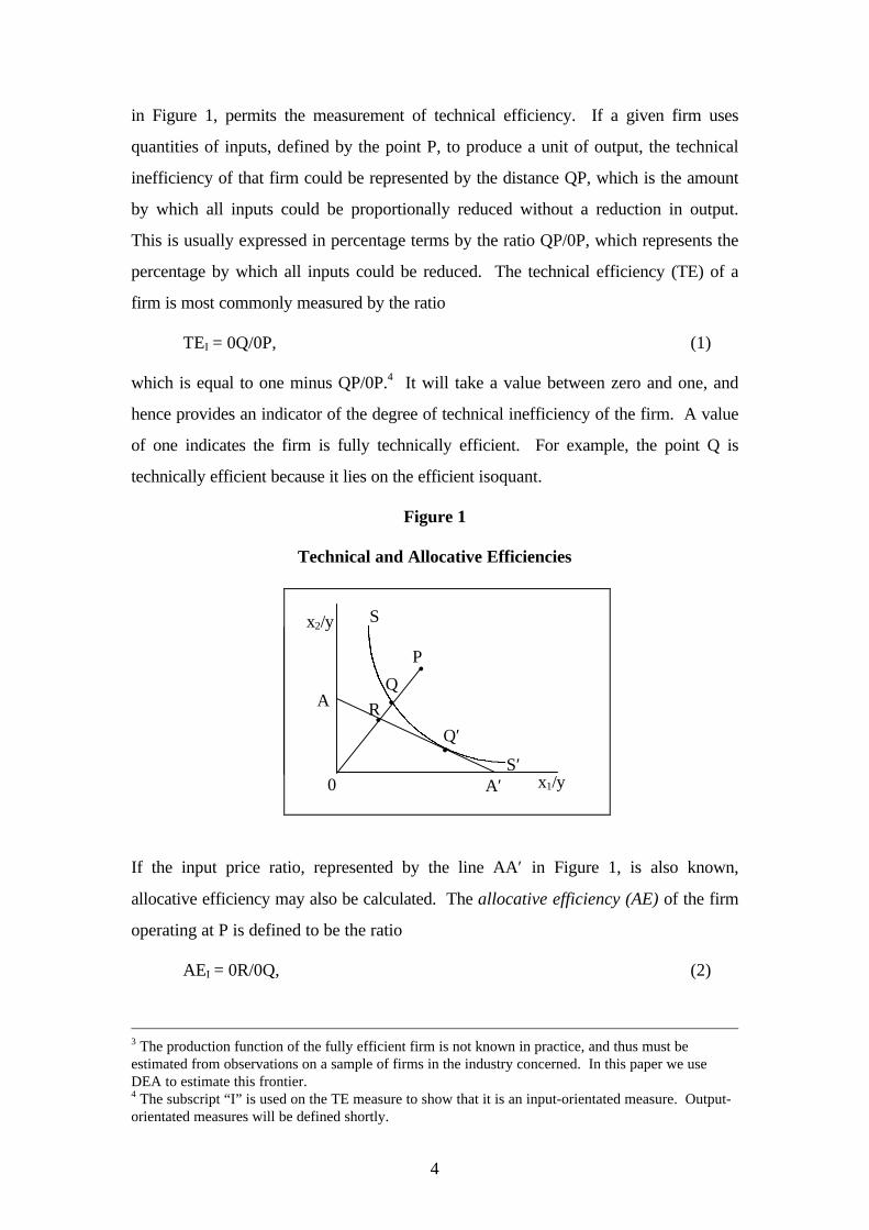
in Figure 1, permits the measurement of technical efficiency. If a given firm uses

quantities of inputs, defined by the point P, to produce a unit of output, the technical

inefficiency of that firm could be represented by the distance QP, which is the amount

by which all inputs could be proportionally reduced without a reduction in output.

This is usually expressed in percentage terms by the ratio QP/0P, which represents the

percentage by which all inputs could be reduced. The technical efficiency (TE) of a

firm is most commonly measured by the ratio

TEI = 0Q/0P, (1)

which is equal to one minus QP/0P.4 It will take a value between zero and one, and

hence provides an indicator of the degree of technical inefficiency of the firm. A value

of one indicates the firm is fully technically efficient. For example, the point Q is

technically efficient because it lies on the efficient isoquant.

Figure 1

Technical and Allocative Efficiencies

If the input price ratio, represented by the line AA′ in Figure 1, is also known,

allocative efficiency may also be calculated. The allocative efficiency (AE) of the firm

operating at P is defined to be the ratio

AEI = 0R/0Q, (2)

3 The production function of the fully efficient firm is not known in practice, and thus must beestimated from observations on a sample of firms in the industry concerned. In this paper we useDEA to estimate this frontier.4 The subscript “I” is used on the TE measure to show that it is an input-orientated measure. Output-orientated measures will be defined shortly.

S

S′

A

A′

P

0

R

Q

Q′

x1/y

x2/y

•

••

•

5

since the distance RQ represents the reduction in production costs that would occur if

production were to occur at the allocatively (and technically) efficient point Q′, instead

of at the technically efficient, but allocatively inefficient, point Q.5

The total economic efficiency (EE) is defined to be the ratio

EEI = 0R/0P, (3)

where the distance RP can also be interpreted in terms of a cost reduction. Note that

the product of technical and allocative efficiency provides the overall economic

efficiency

TEI×AEI = (0Q/0P)×(0R/0Q) = (0R/0P) = EEI. (4)

Note that all three measures are bounded by zero and one.

Figure 2

Piecewise Linear Convex Isoquant

These efficiency measures assume the production function of the fully efficient firm is

known. In practice this is not the case, and the efficient isoquant must be estimated

from the sample data. Farrell suggested the use of either (a) a non-parametric

piecewise-linear convex isoquant constructed such that no observed point should lie to

the left or below it (refer to Figure 2), or (b) a parametric function, such as the Cobb-

Douglas form, fitted to the data, again such that no observed point should lie to the left

or below it. Farrell provided an illustration of his methods using agricultural data for

5 One could illustrate this by drawing two isocost lines through Q and Q′. Irrespective of the slope ofthese two parallel lines (which is determined by the input price ratio) the ratio RQ/0Q would representthe percentage reduction in costs associated with movement from Q to Q′.

•

•

•

•

•

x1/y

x2/y S

S′

0

6

the 48 continental states of the US.

2.2 Output-Orientated Measures

The above input-orientated technical efficiency measure addresses the question: “By

how much can input quantities be proportionally reduced without changing the output

quantities produced?”. One could alternatively ask the question “: “By how much can

output quantities be proportionally expanded without altering the input quantities

used?”. This is an output-orientated measure as opposed to the input-oriented

measure discussed above. The difference between the output- and input-orientated

measures can be illustrated using a simple example involving one input and one output.

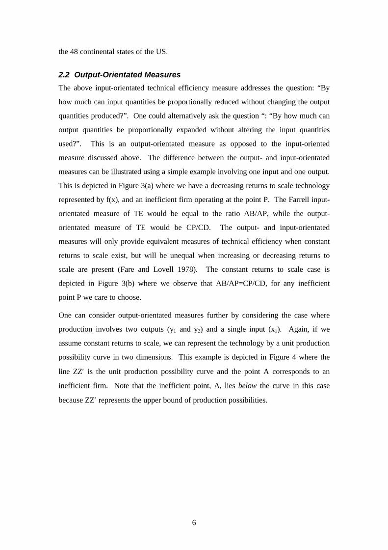
This is depicted in Figure 3(a) where we have a decreasing returns to scale technology

represented by f(x), and an inefficient firm operating at the point P. The Farrell input-

orientated measure of TE would be equal to the ratio AB/AP, while the output-

orientated measure of TE would be CP/CD. The output- and input-orientated

measures will only provide equivalent measures of technical efficiency when constant

returns to scale exist, but will be unequal when increasing or decreasing returns to

scale are present (Fare and Lovell 1978). The constant returns to scale case is

depicted in Figure 3(b) where we observe that AB/AP=CP/CD, for any inefficient

point P we care to choose.

One can consider output-orientated measures further by considering the case where

production involves two outputs (y1 and y2) and a single input (x1). Again, if we

assume constant returns to scale, we can represent the technology by a unit production

possibility curve in two dimensions. This example is depicted in Figure 4 where the

line ZZ′ is the unit production possibility curve and the point A corresponds to an

inefficient firm. Note that the inefficient point, A, lies below the curve in this case

because ZZ′ represents the upper bound of production possibilities.

7

Figure 3

Input- and Output-Orientated Technical Efficiency Measures

and Returns to Scale

Figure 4

Technical and Allocative Efficiencies from an

Output Orientation

The Farrell output-orientated efficiency measures would be defined as follows. In

Figure 4 the distance AB represents technical inefficiency. That is, the amount by

which outputs could be increased without requiring extra inputs. Hence a measure of

output-orientated technical efficiency is the ratio

TEO = 0A/0B. (7)

If we have price information then we can draw the isorevenue line DD′, and define the

allocative efficiency to be

x

y(a) DRTS

BA

C

f(x) f(x)

P

D

•

•

•

x

D

y

D′

(b) CRTS

Z

BA

Z′

C

A

P

0

D

C

•

B

•

B′

•

y1/x

y2/x

••

• •

00

8

AEO = 0B/0C (8)

which has a revenue increasing interpretation (similar to the cost reducing

interpretation of allocative inefficiency in the input-orientated case). Furthermore, one

can define overall economic efficiency as the product of these two measures

EEO = (0A/0C) = (0A/0B)×(0B/0C) = TEO×AEO. (9)

Again, all of these three measures are bounded by zero and one.

Before we conclude this section, two quick points should be made regarding the six

efficiency measures that we have defined:

1) All of them are measured along a ray from the origin to the observed production

point. Hence they hold the relative proportions of inputs (or outputs) constant.

One advantage of these radial efficiency measures is that they are units invariant.

That is, changing the units of measurement (e.g. measuring quantity of labour in

person hours instead of person years) will not change the value of the efficiency

measure. A non-radial measure, such as the shortest distance from the production

point to the production surface, may be argued for, but this measure will not be

invariant to the units of measurement chosen. Changing the units of measurement

in this case could result in the identification of a different “nearest” point. This issue

will be discussed further when we come to consider the treatment of slacks in DEA.

2) The Farrell input- and output-orientated technical efficiency measures can be shown

to be equal to the input and output distance functions discussed in Shepherd (1970).

For more on this see Lovell (1993, p10). This observation becomes important when

we discuss the use of DEA methods in calculating Malmquist indices of TFP

change.

3. Data Envelopment Analysis (DEA)

Data envelopment analysis (DEA) is the non-parametric mathematical programming

approach to frontier estimation. The discussion of DEA models presented here is brief,

with relatively little technical detail. More detailed reviews of the methodology are

presented by Seiford and Thrall (1990), Lovell (1993), Ali and Seiford (1993), Lovell

(1994), Charnes et al (1995) and Seiford (1996).

The piecewise-linear convex hull approach to frontier estimation, proposed by Farrell

9

(1957), was considered by only a handful of authors in the two decades following

Farrell’s paper. Authors such as Boles (1966) and Afriat (1972) suggested

mathematical programming methods which could achieve the task, but the method did

not receive wide attention until a the paper by Charnes, Cooper and Rhodes (1978)

which coined the term data envelopment analysis (DEA). There has since been a large

number of papers which have extended and applied the DEA methodology.

Charnes, Cooper and Rhodes (1978) proposed a model which had an input orientation

and assumed constant returns to scale (CRS).6 Subsequent papers have considered

alternative sets of assumptions, such as Banker, Charnes and Cooper (1984) who

proposed a variable returns to scale (VRS) model. The following discussion of DEA

begins with a description of the input-orientated CRS model in section 3.1, because

this model was the first to be widely applied.

3.1 The Constant Returns to Scale Model (CRS)

We shall begin by defining some notation. Assume there is data on K inputs and M

outputs on each of N firms or DMU’s as they tend to be called in the DEA literature.7

For the i-th DMU these are represented by the vectors xi and yi, respectively. The

K×N input matrix, X, and the M×N output matrix, Y, represent the data of all N

DMU’s. The purpose of DEA is to construct a non-parametric envelopment frontier

over the data points such that all observed points lie on or below the production

frontier. For the simple example of an industry where one output is produced using

two inputs, it can be visualised as a number of intersecting planes forming a tight fitting

cover over a scatter of points in three-dimensional space. Given the CRS assumption,

this can also be represented by a unit isoquant in input/input space (refer to Figure 2).

The best way to introduce DEA is via the ratio form. For each DMU we would like to

obtain a measure of the ratio of all outputs over all inputs, such as u′yi/v′xi, where u is

an M×1 vector of output weights and v is a K×1 vector of input weights. To select

optimal weights we specify the mathematical programming problem:

6 At this point we will begin to use CRS to refer to constant returns to scale rather than CRTS. Mosteconomics texts use the latter, while most DEA papers use the former.7 DMU stands for “decision making unit”. It is a more appropriate term than “firm” when, forexample, a bank is studying the performance of its branches or an education district is studying theperformance of its schools.

10

maxu,v (u′yi/v′xi),

st u′yj/v′xj ≤ 1, j=1,2,...,N,

u, v ≥ 0. (10)

This involves finding values for u and v, such that the efficiency measure of the i-th

DMU is maximised, subject to the constraint that all efficiency measures must be less

than or equal to one. One problem with this particular ratio formulation is that it has

an infinite number of solutions.8 To avoid this one can impose the constraint v′xi = 1,

which provides:

maxµ,ν (µ′yi),

st ν′xi = 1,

µ′yj - ν′xj ≤ 0, j=1,2,...,N,

µ, ν ≥ 0, (11)

where the notation change from u and v to µ and ν reflects the transformation. This

form is known as the multiplier form of the linear programming problem.

Using the duality in linear programming, one can derive an equivalent envelopment

form of this problem:

minθ,λ θ,

st -yi + Yλ ≥ 0,

θxi - Xλ ≥ 0,

λ ≥ 0, (12)

where θ is a scalar and λ is a N×1 vector of constants. This envelopment form

involves fewer constraints than the multiplier form (K+M < N+1), and hence is

generally the preferred form to solve.9 The value of θ obtained will be the efficiency

score for the i-th DMU. It will satisfy θ ≤ 1, with a value of 1 indicating a point on the

8 That is, if (u*,v*) is a solution, then (αu*,αv*) is another solution, etc.9 The forms defined by equations 10 and 11 are introduced here for expository purposes. They are notused again in the remainder of this paper. The multiplier form has, however, been estimated in a

11

frontier and hence a technically efficient DMU, according to the Farrell (1957)

definition. Note that the linear programming problem must be solved N times, once

for each DMU in the sample. A value of θ is then obtained for each DMU.

Slacks

The piecewise linear form of the non-parametric frontier in DEA can cause a few

difficulties in efficiency measurement. The problem arises because of the sections of

the piecewise linear frontier which run parallel to the axes (refer Figure 2) which do

not occur in most parametric functions (refer Figure 1). To illustrate the problem,

refer to Figure 5 where the DMU’s using input combinations C and D are the two

efficient DMU’s which define the frontier, and DMU’s A and B are inefficient

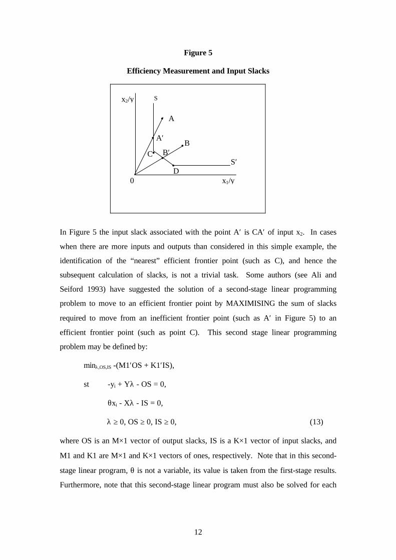
The Farrell (1957) measure of technical efficiency gives the efficiency of DMU’s A and

B as OA′/OA and OB′/OB, respectively. However, it is questionable as to whether the

point A′ is an efficient point since one could reduce the amount of input x2 used (by the

amount CA′) and still produce the same output. This is known as input slack in the

literature.10 Once one considers a case involving more inputs and/or multiple outputs,

the diagrams are no longer as simple, and the possibility of the related concept of

output slack also occurs.11 Thus it could be argued that both the Farrell measure of

technical efficiency (θ) and any non-zero input or output slacks should be reported to

provide an accurate indication of technical efficiency of a DMU in a DEA analysis.12

Note that for the i-th DMU the output slacks will be equal to zero only if Yλ-yi=0,

while the input slacks will be equal to zero only if θxi-Xλ=0 (for the given optimal

values of θ and λ).

number of studies. The µ and ν weights can be interpreted as normalised shadow prices.10 Some authors use the term input excess.11 Output slack is illustrated later in these notes (see Figure 4.8).12 Koopman’s (1951) definition of technical efficiency was stricter than the Farrell (1957) definition.The former is equivalent to stating that a firm is only technically efficient if it operates on the frontierand furthermore that all associated slacks are zero.

12

Figure 5

Efficiency Measurement and Input Slacks

In Figure 5 the input slack associated with the point A′ is CA′ of input x2. In cases

when there are more inputs and outputs than considered in this simple example, the

identification of the “nearest” efficient frontier point (such as C), and hence the

subsequent calculation of slacks, is not a trivial task. Some authors (see Ali and

Seiford 1993) have suggested the solution of a second-stage linear programming

problem to move to an efficient frontier point by MAXIMISING the sum of slacks

required to move from an inefficient frontier point (such as A′ in Figure 5) to an

efficient frontier point (such as point C). This second stage linear programming

problem may be defined by:

minλ,OS,IS -(M1′OS + K1′IS),

st -yi + Yλ - OS = 0,

θxi - Xλ - IS = 0,

λ ≥ 0, OS ≥ 0, IS ≥ 0, (13)

where OS is an M×1 vector of output slacks, IS is a K×1 vector of input slacks, and

M1 and K1 are M×1 and K×1 vectors of ones, respectively. Note that in this second-

stage linear program, θ is not a variable, its value is taken from the first-stage results.

Furthermore, note that this second-stage linear program must also be solved for each

x1/y

x2/y S

S′

0

A

BA′

B′C

D

•

•

••

•

•

13

of the N DMU’s involved.13

There are two major problems associated with this second stage LP. The first and

most obvious problem is that the sum of slacks is MAXIMISED rather than

MINIMISED. Hence it will identify not the NEAREST efficient point but the

FURTHEST efficient point. The second major problem associated with the above

second-stage approach is that it is not invariant to units of measurement. The

alteration of the units of measurement, say for a fertiliser input from kilograms to

tonnes (while leaving other units of measurement unchanged), could result in the

identification of different efficient boundary points and hence different slack and

lambda measures.14

Note, however, that these two issues are not a problem in the simple example

presented in Figure 5 because there is only one efficient point to choose from on the

vertical facet. However, if slack occurs in 2 or more dimensions (which it often does)

then the above mentioned problems can come into play.

As a result of this problem, many studies simply solve the first-stage linear program

(equation 12) for the values of the Farrell radial technical efficiency measures (θ) for

each DMU and ignore the slacks completely, or they report both the radial Farrell

technical efficiency score (θ) and the residual slacks, which may be calculated as

OS = -yi + Yλ and IS = θxi - Xλ. However, this approach is not without problems

either because these residual slacks may not always provide all (Koopmans) slacks

(e.g., when a number of observations appear on the vertical section of the frontier in

Figure 5.5) and hence may not always identify the nearest (Koopmans) efficient point

for each DMU.

In the DEAP software we give the user three choices regarding the treatment of slacks.

These are:

1. One-stage DEA, in which we conduct the LP in equation 12 and calculate slacks

residually;

13 This method is used by all the popular DEA software such as Warwick DEA and IDEAS.14Charnes, Cooper, Rousseau and Semple (1987) suggest a units invariant model where the unit worthof a slack is made inversely proportional to the quantity of that input or output used by the i-th firm.This does solve the immediate problem, but does create another, in that there is no obvious reason forthe slacks to be weighted in this way.

14

2. Two-stage DEA, where we conduct the LP’s in equations 12 and 13; and

3. Multi-stage DEA, where we conduct a sequence of radial LP’s to identify the

efficient projected point.

The multi-stage DEA method is more computationally demanding that the other two

methods(see Coelli 1997 for details). However, the benefits of the approach are that it

identifies efficient projected points which have input and output mixes which are as

similar as possible to those of the inefficient points, and that it is also invariant to units

of measurement. Hence we would recommend the use of the multi-stage method over

the other two alternatives.

Having devoted a number of pages of this manual to the issue of slacks we would like

to conclude by observing that the importance of slacks can be overstated. Slacks may

be viewed as being an artefact of the frontier construction method chosen (DEA) and

the use of finite sample sizes. If an infinite sample size were available and/or if an

alternative frontier construction method was used, which involved a smooth function

surface, the slack issue would disappear. In addition to this observation it also seems

quite reasonable to accept the arguments of Ferrier and Lovell (1990) that slacks may

essentially be viewed as allocative inefficiency. Hence we believe that an analysis of

technical efficiency can reasonably concentrate upon the radial efficiency score

provided in the first stage DEA LP (refer to equation 12). However if one insists on

identifying Koopmans-efficient projected points then we would strongly recommend

the use of the multi-stage method in preference to the two-stage method for the

reasons outlined above.15

Example 1

We will illustrate CRS input-orientated DEA using a simple example involving five

observations on DMU’s (firms) which use two inputs to produce a single output. The

data is as follows:

15 However we have also included the 2-stage option in our software because it is the method used inother popular DEA software packages such as Warwick DEA and IDEAS.

15

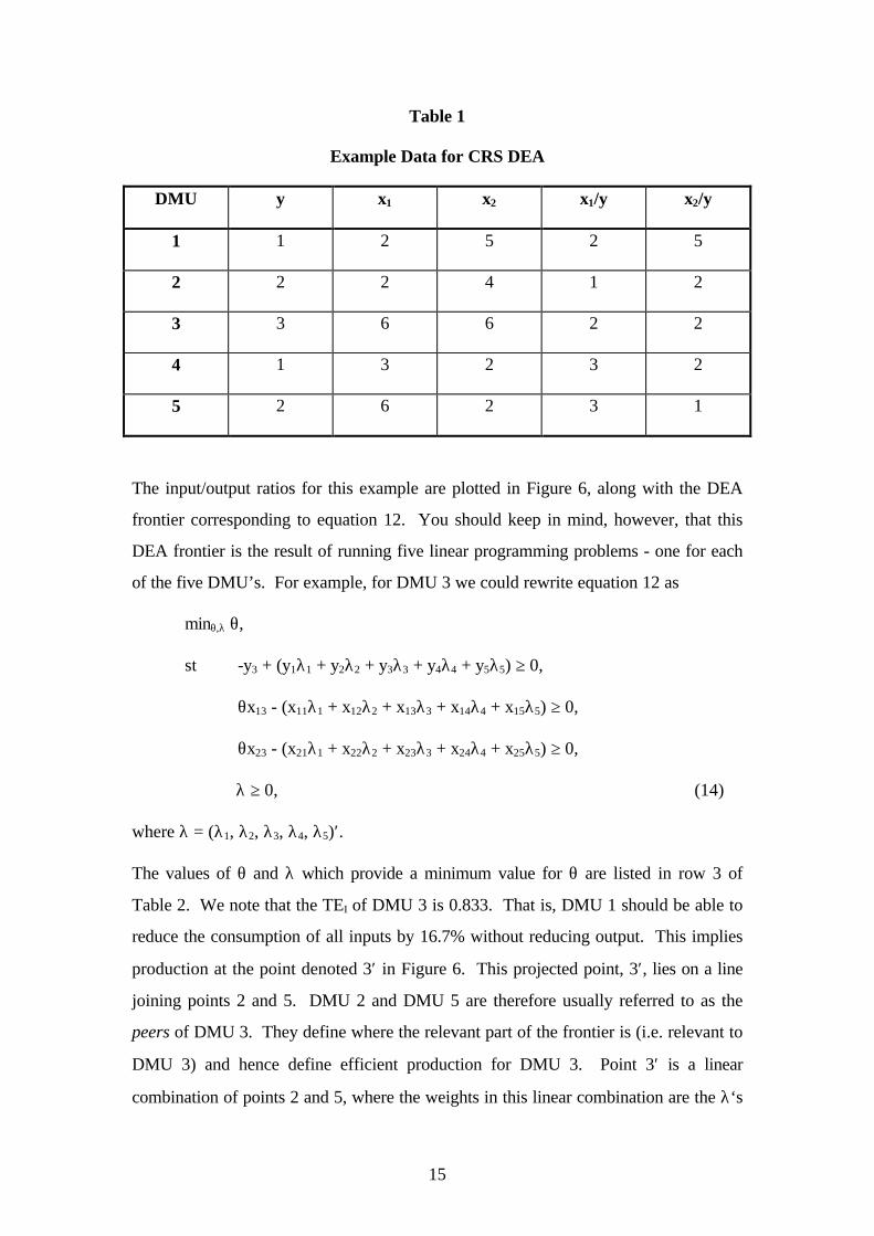
Table 1

Example Data for CRS DEA

DMU y x1 x2 x1/y x2/y

1 1 2 5 2 5

2 2 2 4 1 2

3 3 6 6 2 2

4 1 3 2 3 2

5 2 6 2 3 1

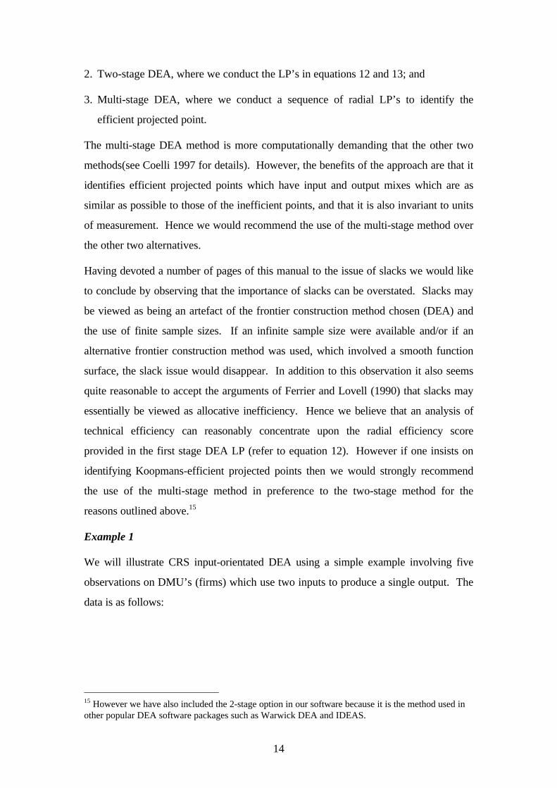
The input/output ratios for this example are plotted in Figure 6, along with the DEA

frontier corresponding to equation 12. You should keep in mind, however, that this

DEA frontier is the result of running five linear programming problems - one for each

of the five DMU’s. For example, for DMU 3 we could rewrite equation 12 as

minθ,λ θ,

st -y3 + (y1λ1 + y2λ2 + y3λ3 + y4λ4 + y5λ5) ≥ 0,

θx13 - (x11λ1 + x12λ2 + x13λ3 + x14λ4 + x15λ5) ≥ 0,

θx23 - (x21λ1 + x22λ2 + x23λ3 + x24λ4 + x25λ5) ≥ 0,

λ ≥ 0, (14)

where λ = (λ1, λ2, λ3, λ4, λ5)′.

The values of θ and λ which provide a minimum value for θ are listed in row 3 of

Table 2. We note that the TEI of DMU 3 is 0.833. That is, DMU 1 should be able to

reduce the consumption of all inputs by 16.7% without reducing output. This implies

production at the point denoted 3′ in Figure 6. This projected point, 3′, lies on a line

joining points 2 and 5. DMU 2 and DMU 5 are therefore usually referred to as the

peers of DMU 3. They define where the relevant part of the frontier is (i.e. relevant to

DMU 3) and hence define efficient production for DMU 3. Point 3′ is a linear

combination of points 2 and 5, where the weights in this linear combination are the λ‘s

16

in row 3 of Table 2.

Figure 6

CRS Input-Orientated DEA Example

x2/y

x1/y

0

1

2

3

4

5

6

0 1 2 3 4 5 6

Table 2

CRS Input-Orientated DEA Results

DMU θθ λλ1 λλ2 λλ3 λλ4 λλ5 IS1 IS2 OS

1 0.5 - 0.5 - - - - 0.5 -

2 1.0 - 1.0 - - - - - -

3 0.833 - 1.0 - - 0.5 - - -

4 0.714 - 0.214 - - 0.286 - - -

5 1.0 - - - - 1.0 - - -

Many DEA studies also talk about targets as well as peers. The targets of DMU 3 are

54′

43

3′

21′

1

FRONTIER¡

¡

¡

17

the coordinates of the efficient projection point 3′. These are equal to 0.833×(2,2) =

(1.666,1.666). Thus DMU 3 should aim to produce its 3 units of output with

3×(1.666,1.666) = (5,5) units of the two inputs.

One could go through a similar discussion of the other two inefficient DMU’s. DMU

4 has TEI = 0.714 and has the same peers as DMU 3. DMU 1 has TEI = 0.5 and has

DMU 2 as its peer. You will also note that the projected point for DMU 1 (1′) lies

upon part of the frontier which is parallel to the x2 axis. Thus it does not represent an

efficient point (according to Koopman’s definition) because we could decrease the use

of the input x2 by 0.5 units (thus producing at the point 2) and still produce the same

output. Thus DMU 1 is said to be radially inefficient in input usage by a factor of 50%

plus it has (non-radial) input slack of 0.5 units of x2. The targets of DMU 1 would

therefore be to reduce usage of both inputs by 50% and also to reduce the use of x2 by

a further 0.5 units. This would result in targets of (x1=1,x2=2). That is, the

coordinates of point 2.

A quick glance at Table 2 shows that DMU’s 2 and 5 have TEI values of 1.0 and that

their peers are themselves. This is as one would expect for the efficient points which

define the frontier.

3.2 The Variable Returns to Scale Model (VRS) and Scale Efficiencies

The CRS assumption is only appropriate when all DMU’s are operating at an optimal

scale (i.e one corresponding to the flat portion of the LRAC curve). Imperfect

competition, constraints on finance, etc. may cause a DMU to be not operating at

optimal scale. Banker, Charnes and Cooper(1984) suggested an extension of the CRS

DEA model to account for variable returns to scale (VRS) situations. The use of the

CRS specification when not all DMU’s are operating at the optimal scale, will result in

measures of TE which are confounded by scale efficiencies (SE). The use of the VRS

specification will permit the calculation of TE devoid of these SE effects.

The CRS linear programming problem can be easily modified to account for VRS by

adding the convexity constraint: N1′λ=1 to (12) to provide:

minθ,λ θ,

st -yi + Yλ ≥ 0,

18

θxi - Xλ ≥ 0,

N1′λ=1

λ ≥ 0, (15)

where N1 is an N×1 vector of ones. This approach forms a convex hull of intersecting

planes which envelope the data points more tightly than the CRS conical hull and thus

provides technical efficiency scores which are greater than or equal to those obtained

using the CRS model. The VRS specification has been the most commonly used

specification in the 1990’s.

Calculation of Scale Efficiencies

Many studies have decomposed the TE scores obtained from a CRS DEA into two

components, one due to scale inefficiency and one due to “pure” technical inefficiency.

This may be done by conducting both a CRS and a VRS DEA upon the same data. If

there is a difference in the two TE scores for a particular DMU, then this indicates that

the DMU has scale inefficiency, and that the scale inefficiency can be calculated from

the difference between the VRS TE score and the CRS TE score.

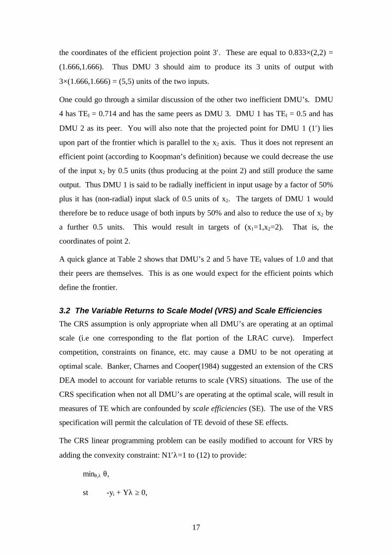
Figure 7 attempts to illustrate this. In this figure we have a one-input one-output

example and have drawn the CRS and VRS DEA frontiers. Under CRS the input-

orientated technical inefficiency of the point P is the distance PPC, while under VRS

the technical inefficiency would only be PPV. The difference between these two, PCPV,

is put down to scale inefficiency. One can also express all of this in ratio efficiency

measures as:

TEI,CRS = APC/AP

TEI,VRS = APV/AP

SEI = APC/APV

where all of these measures will be bounded by zero and one. We also note that

TEI,CRS = TEI,VRS×SEI

because

APC/AP = (APV/AP)×(APC/APV).

19

That is, the CRS technical efficiency measure is decomposed into “pure” technical

efficiency and scale efficiency.

Figure 7

Calculation of Scale Economies in DEA

One shortcoming of this measure of scale efficiency is that the value does not indicate

whether the DMU is operating in an area of increasing or the decreasing returns to

scale. This may be determined by running an addition DEA problem with non-

increasing returns to scale (NIRS) imposed. This can be done by altering the DEA

model in equation 15 by substituting the N1′λ=1 restriction with N1′λ ≤ 1, to provide:

minθ,λ θ,

st -yi + Yλ ≥ 0,

θxi - Xλ ≥ 0,

N1′λ ≤ 1

λ ≥ 0, (16)

The NIRS DEA frontier is also plotted in Figure 7. The nature of the scale

inefficiencies (i.e. due to increasing or decreasing returns to scale) for a particular

DMU can be determined by seeing whether the NIRS TE score is equal to the VRS TE

score. If they are unequal (as will be the case for the point P in Figure 7) then

increasing returns to scale exist for that DMU. If they are equal (as is the case for

0

y

x

Q

PPC

A

•

••• •

•

•

CRSNIRS

VRS

PV

20

point Q in Figure 7) then decreasing returns to scale apply. An example of this

approach applied to international airlines is provided in BIE (1994).

Example 2

This is a simple numerical example involving five firms which produce a single output

using a single input. The data are listed in Table 3 and the VRS and CRS input-

orientated DEA results are listed in Table 4 and plotted in Figure 8. Given that we are

using an input orientation, the efficiencies are measured horizontally across Figure 8.

We observe that firm 3 is the only efficient firm (i.e., on the DEA frontier) when CRS

is assumed but that firms 1, 3 and 5 are efficient when VRS is assumed.

The calculation of the various efficiency measures can be illustrated using firm 2 which

is inefficient under both CRS and VRS technologies. The CRS technical efficiency

(TE) is equal to 2/4=0.5; the VRS TE is 2.5/4=0.625 and the scale efficiency is equal

to the ratio of the CRS TE to the VRS TE which is 0.5/0.625=0.8. We also observe

that firm 2 is on the increasing returns to scale (IRS) portion of the VRS frontier.

Table 3

Example Data for VRS DEA

DMU y x

1 1 2

2 2 4

3 3 3

4 5 5

5 5 6

21

Table 4

VRS Input-Orientated DEA Results

DMU CRS TE VRS TE SCALE

1 0.500 1.000 0.500 irs

2 0.500 0.625 0.800 irs

3 1.000 1.000 1.000 -

4 0.800 0.900 0.889 drs

5 0.833 1.000 0.833 drs

mean 0.727 0.905 0.804

Figure 8

VRS Input-Orientated DEA Example

x

y

0

1

2

3

4

5

6

0 1 2 3 4 5 6 7

5

4

3

2

1

CRS DEA

VRS DEA

22

3.3 Input and Output Orientations

In the preceding input-orientated models, discussed in sections 3.1 and 3.2, the method

sought to identify technical inefficiency as a proportional reduction in input usage.

This corresponds to Farrell’s input-based measure of technical inefficiency. As

discussed in section 2.2, it is also possible to measure technical inefficiency as a

proportional increase in output production. The two measures provide the same value

under CRS but are unequal when VRS is assumed (see Figure 3). Given that linear

programming cannot suffer from such statistical problems as simultaneous equation

bias, the choice of an appropriate orientation is not as crucial as it is in the econometric

estimation case. In many studies the analysts have tended to select input-orientated

models because many DMU’s have particular orders to fill (e.g. electricity generation)

and hence the input quantities appear to be the primary decision variables, although

this argument may not be as strong in all industries. In some industries the DMUs may

be given a fixed quantity of resources and asked to produce as much output as

possible. In this case an output orientation would be more appropriate. Essentially

one should select an orientation according to which quantities (inputs or outputs) the

managers have most control over. Furthermore, in many instances you will observe

that the choice of orientation will have only minor influences upon the scores obtained

(e.g. see Coelli and Perelman 1996).

The output-orientated models are very similar to their input-orientated counterparts.

Consider the example of the following output-orientated VRS model:

maxφ,λ φ,

st -φyi + Yλ ≥ 0,

xi - Xλ ≥ 0,

N1′λ=1

λ ≥ 0, (17)

where 1≤φ<∞, and φ-1 is the proportional increase in outputs that could be achieved by

the i-th DMU, with input quantities held constant.16 Note that 1/φ defines a TE score

which varies between zero and one (and that this is the output-orientated TE score

16 An output-oriented CRS model is defined in a similar way, but is not presented here for brevity.

23

reported by DEAP).

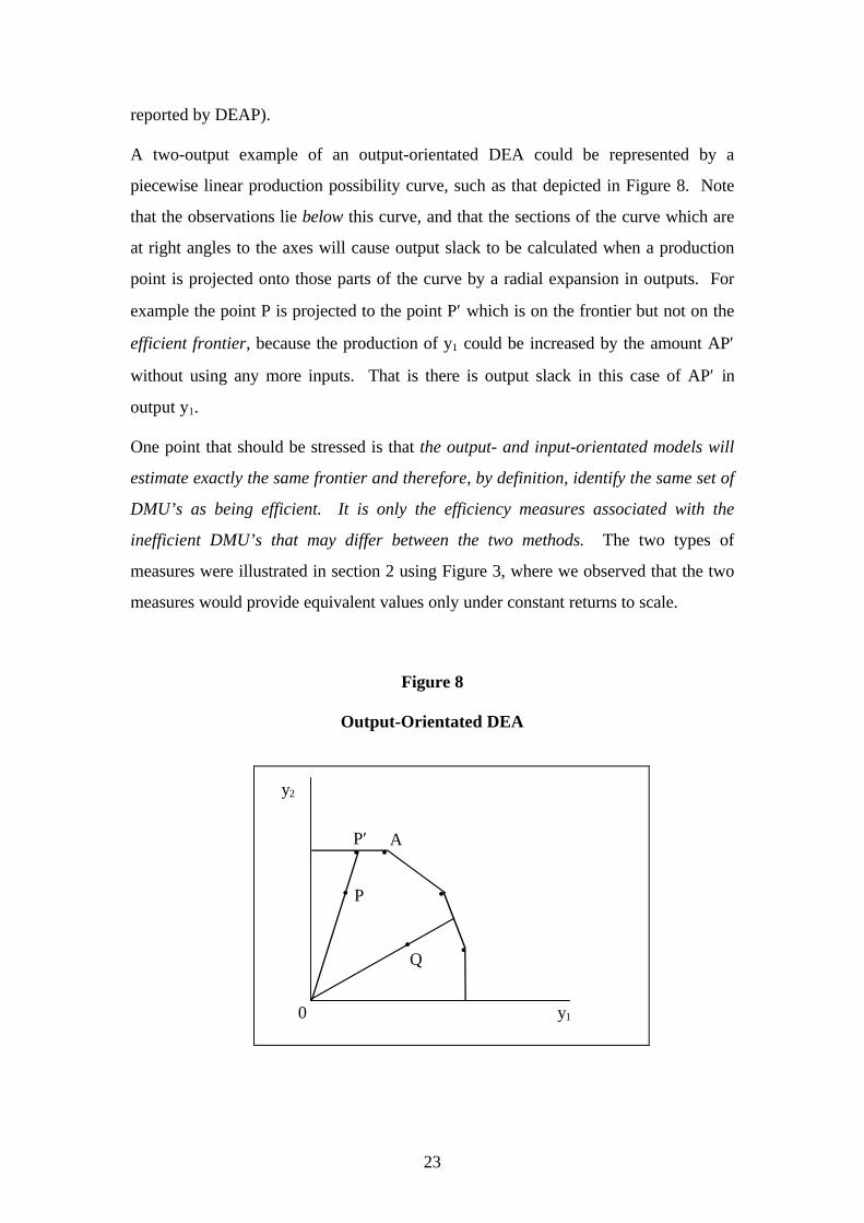
A two-output example of an output-orientated DEA could be represented by a

piecewise linear production possibility curve, such as that depicted in Figure 8. Note

that the observations lie below this curve, and that the sections of the curve which are

at right angles to the axes will cause output slack to be calculated when a production

point is projected onto those parts of the curve by a radial expansion in outputs. For

example the point P is projected to the point P′ which is on the frontier but not on the

efficient frontier, because the production of y1 could be increased by the amount AP′

without using any more inputs. That is there is output slack in this case of AP′ in

output y1.

One point that should be stressed is that the output- and input-orientated models will

estimate exactly the same frontier and therefore, by definition, identify the same set of

DMU’s as being efficient. It is only the efficiency measures associated with the

inefficient DMU’s that may differ between the two methods. The two types of

measures were illustrated in section 2 using Figure 3, where we observed that the two

measures would provide equivalent values only under constant returns to scale.

Figure 8

Output-Orientated DEA

0

y2

y1

Q

P′

P

A

•

•

• •

•

•

24

3.4 Price Information and Allocative Efficiency

If one has price information and is willing to consider a behavioural objective, such as

cost minimisation or revenue maximisation, then one can measure both technical and

allocative efficiencies. For the case of VRS cost minimisation, one would run the

input-orientated DEA model set out in equation 15 to obtain technical efficiencies

(TE). One would then run the following cost minimisation DEA

minλ,xi* wi′xi*,

st -yi + Yλ ≥ 0,

xi* - Xλ ≥ 0,

N1′λ=1

λ ≥ 0, (23)

where wi is a vector of input prices for the i-th DMU and xi* (which is calculated by

the LP) is the cost-minimising vector of input quantities for the i-th DMU, given the

input prices wi and the output levels yi. The total cost efficiency (CE) or economic

efficiency of the i-th DMU would be calculated as

CE = wi′xi*/ wi′xi.

That is, the ratio of minimum cost to observed cost. One can then use equation 4 to

calculate the allocative efficiency residually as

AE = CE/TE.

Note that this procedure will include any slacks into the allocative efficiency measure.

This is often justified on the grounds that slack reflects an inappropriate input mix (see

Ferrier and Lovell, 1990, p235).

Note also that one can also consider revenue maximisation and allocative inefficiency

in output mix selection in a similar manner. See Lovell (1993, p33) for a discussion of

this. Note that this revenue efficiency model is not implemented in DEAP.

Example 3

In this example we take the data from Example 1 and add the information that all firms

face the same prices which are 1 and 3 for inputs 1 and 2, respectively. Thus if we

draw an isocost line with a slope of -1/3 onto Figure 6 which is tangential to the

25

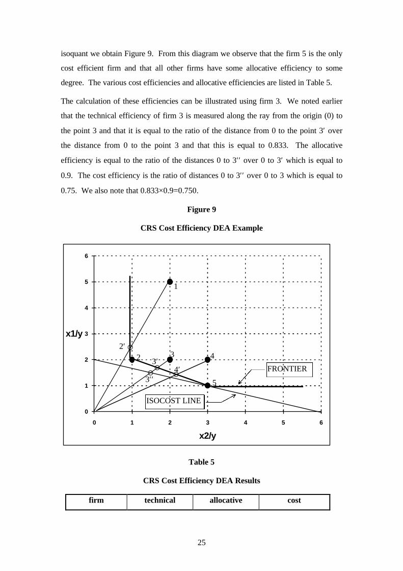
isoquant we obtain Figure 9. From this diagram we observe that the firm 5 is the only

cost efficient firm and that all other firms have some allocative efficiency to some

degree. The various cost efficiencies and allocative efficiencies are listed in Table 5.

The calculation of these efficiencies can be illustrated using firm 3. We noted earlier

that the technical efficiency of firm 3 is measured along the ray from the origin (0) to

the point 3 and that it is equal to the ratio of the distance from 0 to the point 3′ over

the distance from 0 to the point 3 and that this is equal to 0.833. The allocative

efficiency is equal to the ratio of the distances 0 to 3′′ over 0 to 3′ which is equal to

0.9. The cost efficiency is the ratio of distances 0 to 3′′ over 0 to 3 which is equal to

0.75. We also note that 0.833×0.9=0.750.

Figure 9

CRS Cost Efficiency DEA Example

x2/y

x1/y

0

1

2

3

4

5

6

0 1 2 3 4 5 6

Table 5

CRS Cost Efficiency DEA Results

firm technical allocative cost

5

4

4′

3

3′′

3′22′

1

FRONTIER

¡

¡¡¡

ISOCOST LINE

26

efficiency efficiency efficiency

1 0.500 0.706 0.353

2 1.000 0.857 0.857

3 0.833 0.900 0.750

4 0.714 0.933 0.667

5 1.000 1.000 1.000

mean 0.810 0.879 0.725

3.5 Panel Data, DEA and the Malmquist Index

When one has panel data, one may use DEA-like linear programs and a (input- or

output-based) Malmquist TFP index to measure productivity change, and to

decompose this productivity change into technical change and technical efficiency

change.

Fare et al (1994) specifies an output-based Malmquist productivity change index17 as:

( ) ( )( )

( )( )

m y x y xd x y

d x y

d x y

d x yo t t t tot

t t

ot

t t

ot

t t

ot

t t+ +

+ ++

+ ++= ×

1 1

1 11

1 1

1

1 2

, , ,,

,

,

,

/

. (24)

This represents the productivity of the production point (xt+1, yt+1) relative to the

production point (xt, yt). A value greater than one will indicate positive TFP growth

from period t to period t+1. This index is, in fact, the geometric mean of two output-

based Malmquist TFP indices. One index uses period t technology and the other

period t+1 technology. To calculate equation 24 we must calculate the four

component distance functions, which will involve four LP problems (similar to those

conducted in calculating Farrell technical efficiency (TE) measures).

We begin by assuming CRS technology (we conduct a further decomposition later to

look at scale efficiency questions). The CRS output-orientated LP used to calculate

dot(xt, yt) is identical to equation 17, except that the convexity (VRS) restriction has

been removed and time subscripts have been included. That is,

17 The subscript “o” has been introduced to remind us that these are output-orientated measures. Notethat input-orientated Malmquist TFP indices can also be defined in a similar way to the output-orientated measures presented here (see Grosskopf, 1993, p183).

27

[dot(xt, yt)]

-1 = maxφ,λ φ,

st -φyit + Ytλ ≥ 0,

xit - Xtλ ≥ 0,

λ ≥ 0, (25)

The remaining three LP problems are simple variants of this:

[dot+1(xt+1, yt+1)]

-1 = maxφ,λ φ,

st -φyi,t+1 + Yt+1λ ≥ 0,

xi,t+1 - Xt+1λ ≥ 0,

λ ≥ 0, (26)

[dot(xt+1, yt+1)]

-1 = maxφ,λ φ,

st -φyi,t+1 + Ytλ ≥ 0,

xi,t+1 - Xtλ ≥ 0,

λ ≥ 0, (27)

[dot+1(xt, yt)]

-1 = maxφ,λ φ,

st -φyit + Yt+1λ ≥ 0,

xit - Xt+1λ ≥ 0,

λ ≥ 0, (28)

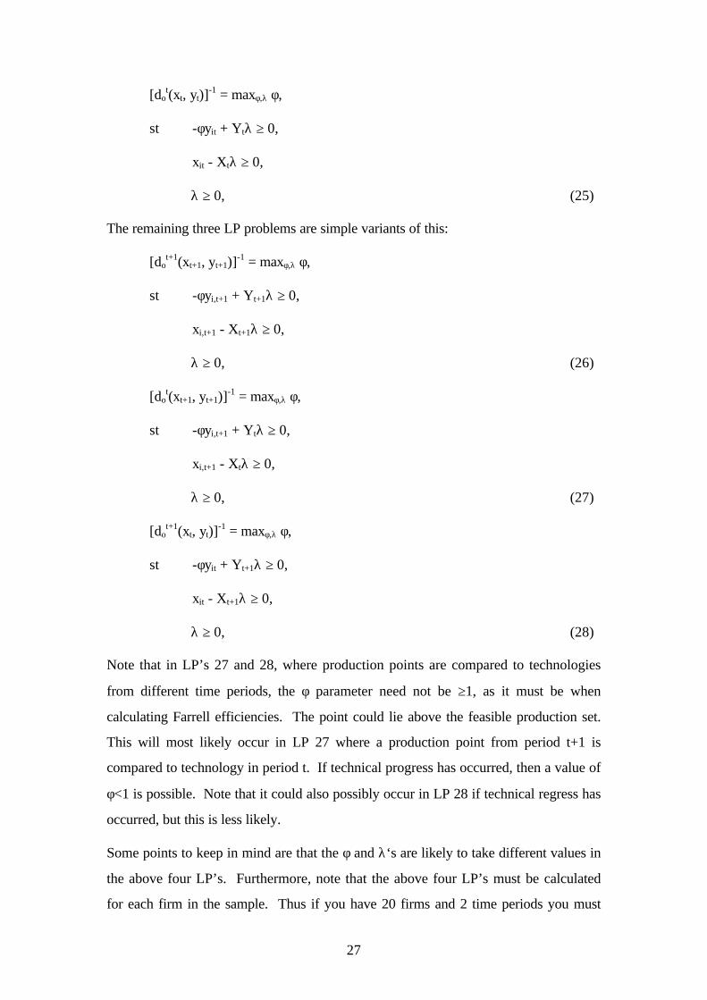
Note that in LP’s 27 and 28, where production points are compared to technologies

from different time periods, the φ parameter need not be ≥1, as it must be when

calculating Farrell efficiencies. The point could lie above the feasible production set.

This will most likely occur in LP 27 where a production point from period t+1 is

compared to technology in period t. If technical progress has occurred, then a value of

φ<1 is possible. Note that it could also possibly occur in LP 28 if technical regress has

occurred, but this is less likely.

Some points to keep in mind are that the φ and λ‘s are likely to take different values in

the above four LP’s. Furthermore, note that the above four LP’s must be calculated

for each firm in the sample. Thus if you have 20 firms and 2 time periods you must

28

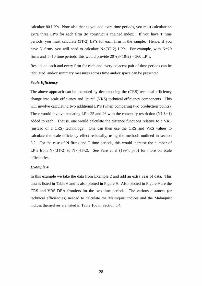
calculate 80 LP’s. Note also that as you add extra time periods, you must calculate an

extra three LP’s for each firm (to construct a chained index). If you have T time

periods, you must calculate (3T-2) LP’s for each firm in the sample. Hence, if you

have N firms, you will need to calculate N×(3T-2) LP’s. For example, with N=20

firms and T=10 time periods, this would provide 20×(3×10-2) = 560 LP’s.

Results on each and every firm for each and every adjacent pair of time periods can be

tabulated, and/or summary measures across time and/or space can be presented.

Scale Efficiency

The above approach can be extended by decomposing the (CRS) technical efficiency

change into scale efficiency and “pure” (VRS) technical efficiency components. This

will involve calculating two additional LP’s (when comparing two production points).

These would involve repeating LP’s 25 and 26 with the convexity restriction (N1′λ=1)

added to each. That is, one would calculate the distance functions relative to a VRS

(instead of a CRS) technology. One can then use the CRS and VRS values to

calculate the scale efficiency effect residually, using the methods outlined in section

3.2. For the case of N firms and T time periods, this would increase the number of

LP’s from N×(3T-2) to N×(4T-2). See Fare et al (1994, p75) for more on scale

efficiencies.

Example 4

In this example we take the data from Example 2 and add an extra year of data. This

data is listed in Table 6 and is also plotted in Figure 9. Also plotted in Figure 9 are the

CRS and VRS DEA frontiers for the two time periods. The various distances (or

technical efficiencies) needed to calculate the Malmquist indices and the Malmquist

indices themselves are listed in Table 10c in Section 5.4.

29

Table 6

Example Data for Malmquist DEA

DMU year y x

1 1 1 2

2 1 2 4

3 1 3 3

4 1 5 5

5 1 5 6

1 2 1 2

2 2 3 4

3 2 4 3

4 2 5 5

5 2 5 5

Figure 8

VRS Input-Orientated DEA Example

x

y

0

1

2

3

4

5

6

0 1 2 3 4 5 6 7

year 1 year 2

5 5

4

43

3 2

2

1

CRS DEAYEAR 1

VRS DEAYEAR 1

CRS DEAYEAR 2 VRS DEA

YEAR 2

30

4. The DEAP Computer Program

This section describes the use of the DEAP computer program. This program is

written in Fortran (Lahey F77LEM/32) for IBM compatible PCs. It is a DOS program

but can be easily run from WINDOWS using FILE MANAGER. The program

involves a simple batch file system where the user creates a data file and a small file

containing instructions. The user then starts the program by typing “DEAP” at the

DOS prompt18 and is then prompted for the name of the instruction file. The program

then executes these instructions and produces an output file which can be read using a

text editor, such as NOTEPAD or EDIT, or using a word processor, such as WORD

or WORD PERFECT.

The execution of DEAP Version 2.0 on an IBM PC generally involves five files:

1) The executable file DEAP.EXE

2) The start-up file DEAP.000

3) A data file (for example, called TEST.DTA)

4) An instruction file (for example, called TEST.INS)

5) An output file (for example, called TEST.OUT).

The executable file and the start-up file is supplied on the disk. The start-up file,

DEAP.000, is a file which stores key parameter values which the user may or may not

need to alter.19 The data and instruction files must be created by the user prior to

execution. The output file is created by DEAP during execution. Examples of data,

instruction and output files are listed in the next section.

Data file

The program requires that the data be listed in a text file20 and expects the data to

appear in a particular order. The data must be listed by observation (i.e., one row for

each firm). There must be a column for each output and each input, with all outputs

listed first and then all inputs listed (from left to right across the file). For example, if

you have 40 observations on two outputs and two inputs there would be four columns

18 The program can also be run by double-clicking on the DEAP.EXE file in FILE MANAGER inWINDOWS.19 At present this file only contains the value of a variable used to test inequalities with zero. This textfile may be edited if the user wishes to alter this value.

31

of data (each of length 40) listed in the order: y1, y2, x1, x2.

If you choose the cost efficiencies option you will also need to supply price

information for the inputs. These price columns should be listed to the right of the

input data columns and appear in the same order. That is, if you have three outputs

and two inputs, the order for the columns should be: y1, y2, y3, x1, x2, w1, w2, where

w1 and w2 are input prices corresponding to input quantities x1 and x2.

If you choose the Malmquist option you will be dealing with panel data. For example,

you may have 30 firms observed in each of 4 years. In this instance you must list all

data for year 1 first, followed by the year 2 data listed in the same order (of firms) and

so on. Note that the panel must be “balanced”. That is, all firms must be observed in

all time periods.

A data file can be produced using any number of computer packages. For example:

• using a text editor (such as DOS EDIT or NOTEPAD),

• using a word processor (such as WORD or WORD PERFECT) and saving

the file in text format,

• using a spreadsheet (such as LOTUS or EXCEL) and printing to a file, or

• using a statistics package (such as SHAZAM or SAS) and writing data to a

file.

Note that the data file should only contain numbers separated by spaces or tabs. It

should not contain any column headings.

Instruction file

The instruction file is a text file which is usually constructed using a text editor or a

word processor. The easiest way to create an instruction file is to make a copy of the

DBLANK.INS file which is supplied with the program (by using the FILE/COPY

menus in FILE MANAGER in WINDOWS or by using the COPY command at the

DOS prompt). We then edit this file (using a text editor or word processor) and type

in the relevant information. The best way to describe the structure of the instruction

file is to provide a few examples. These are listed in the following section.

20 All data, instruction and output files are (ASCII) text files.

32

Output file

As noted earlier, the output file is a text file which is produced by DEAP when an

instruction file is executed. The output file can be read using a text editor, such as

NOTEPAD or EDIT, or using a word processor, such as WORD or WORD

PERFECT. The output may also be imported into a spreadsheet program, such as

EXCEL or LOTUS, to allow further manipulation into tables and graphs for

subsequent inclusion into report documents.

5. Examples

In this section we shall consider four examples:

1) An input-orientated CRS DEA involving five observations on one output

and two inputs..

2) An input-orientated VRS DEA involving five observations on one output

and one input.

3) A CRS cost efficiency DEA using the data from example (1) along with

some input price data.

4) An output-orientated Malmquist DEA involving data on one output and one

input for 5 firms observed over a three year period.

These examples correspond to the four examples discussed in Section 3.

5.1 Example 1: An Input-orientated CRS DEA Example

The text file EG1.DTA (refer to Table 7a) contains five observations on one output

and two inputs. The output is listed in the first column and the inputs in the next two

columns. This data is identical to that listed in Table 1.

The EG1.INS file is listed in Table 7b. The purpose of the majority of entries in the

file should be self explanatory, due to the comments on the right-hand side of the file.21

The first two lines of the file contain the name of the data file (EG1.DTA) and an

output file name (here we have used EG1.OUT). Then on the next four lines we

21It should be mentioned that the comments in DBLANK.INS and DEAP.000 are not read by theprogram. Hence users may have instruction files which are made from scratch with a text editor andwhich contain no comments. This is not recommended, however, as it would be too easy to lose trackof which input value belongs on which line.

33

specify the number of firms (5); number of time periods (1);22 number of outputs (1);

and number of inputs (2). On the final three lines we specify a “0” to indicate CRS; a

“0” to indicate an input orientation; and a “0” to indicate that we wish to estimate a

standard DEA model.23

Finally we type “DEAP” at the DOS prompt, and then type in the name of the

instruction file (EG1.INS). The program will then take somewhere between a few

seconds and a few minutes (depending upon the size of the model and the speed of

your computer) to run the required LP problems and send the output to the file you

have named (EG1.OUT). This file is reproduced in Table 7c. These results are

identical to those presented in Table 2.

Table 7a - Listing of Data File EG1.DTA_____________________________________________________________________1 2 52 2 43 6 61 3 22 6 2

_____________________________________________________________________

Table 7b - Listing of Instruction File EG1.INS_____________________________________________________________________eg1.dta DATA FILE NAMEeg1.out OUTPUT FILE NAME5 NUMBER OF FIRMS1 NUMBER OF TIME PERIODS1 NUMBER OF OUTPUTS2 NUMBER OF INPUTS0 0=INPUT AND 1=OUTPUT ORIENTATED0 0=CRS AND 1=VRS0 0=DEA(MULTI-STAGE), 1=COST-DEA, 2=MALMQUIST-DEA,

3=DEA(1-STAGE), 4=DEA(2-STAGE)

_____________________________________________________________________

Table 7c - Listing of Output File EG1.OUT_____________________________________________________________________Results from DEAP Version 2.1

Instruction file = eg1.insData file = eg1.dta

22 Note that the number of time periods will always be equal to 1 unless the Malmquist DEA option isselected.23 Note that by specifying “0” on the final line we are asking that slacks be calculated using the multi-stage method. If we wished the 1-stage or 2-stage methods to be used we would have used a “3” or a

34

Input orientated DEA

Scale assumption: CRS

Slacks calculated using multi-stage method

EFFICIENCY SUMMARY:

firm te 1 0.500 2 1.000 3 0.833 4 0.714 5 1.000

mean 0.810

SUMMARY OF OUTPUT SLACKS:

firm output: 1 1 0.000 2 0.000 3 0.000 4 0.000 5 0.000

mean 0.000

SUMMARY OF INPUT SLACKS:

firm input: 1 2 1 0.000 0.500 2 0.000 0.000 3 0.000 0.000 4 0.000 0.000 5 0.000 0.000

mean 0.000 0.100

SUMMARY OF PEERS:

firm peers: 1 2 2 2 3 5 2 4 5 2 5 5

SUMMARY OF PEER WEIGHTS: (in same order as above)

firm peer weights: 1 0.500 2 1.000 3 0.500 1.000 4 0.286 0.214 5 1.000

35

PEER COUNT SUMMARY: (i.e., no. times each firm is a peer for another)

firm peer count: 1 0 2 3 3 0 4 0 5 2

SUMMARY OF OUTPUT TARGETS:

firm output: 1 1 1.000 2 2.000 3 3.000 4 1.000 5 2.000

SUMMARY OF INPUT TARGETS:

firm input: 1 2 1 1.000 2.000 2 2.000 4.000 3 5.000 5.000 4 2.143 1.429 5 6.000 2.000

FIRM BY FIRM RESULTS:

Results for firm: 1Technical efficiency = 0.500PROJECTION SUMMARY: variable original radial slack projected value movement movement value output 1 1.000 0.000 0.000 1.000 input 1 2.000 -1.000 0.000 1.000 input 2 5.000 -2.500 -0.500 2.000LISTING OF PEERS: peer lambda weight 2 0.500

Results for firm: 2Technical efficiency = 1.000PROJECTION SUMMARY: variable original radial slack projected value movement movement value output 1 2.000 0.000 0.000 2.000 input 1 2.000 0.000 0.000 2.000 input 2 4.000 0.000 0.000 4.000LISTING OF PEERS: peer lambda weight 2 1.000

Results for firm: 3

36

Technical efficiency = 0.833PROJECTION SUMMARY: variable original radial slack projected value movement movement value output 1 3.000 0.000 0.000 3.000 input 1 6.000 -1.000 0.000 5.000 input 2 6.000 -1.000 0.000 5.000LISTING OF PEERS: peer lambda weight 5 0.500 2 1.000

Results for firm: 4Technical efficiency = 0.714PROJECTION SUMMARY: variable original radial slack projected value movement movement value output 1 1.000 0.000 0.000 1.000 input 1 3.000 -0.857 0.000 2.143 input 2 2.000 -0.571 0.000 1.429LISTING OF PEERS: peer lambda weight 5 0.286 2 0.214

Results for firm: 5Technical efficiency = 1.000PROJECTION SUMMARY: variable original radial slack projected value movement movement value output 1 2.000 0.000 0.000 2.000 input 1 6.000 0.000 0.000 6.000 input 2 2.000 0.000 0.000 2.000LISTING OF PEERS: peer lambda weight 5 1.000

_____________________________________________________________________

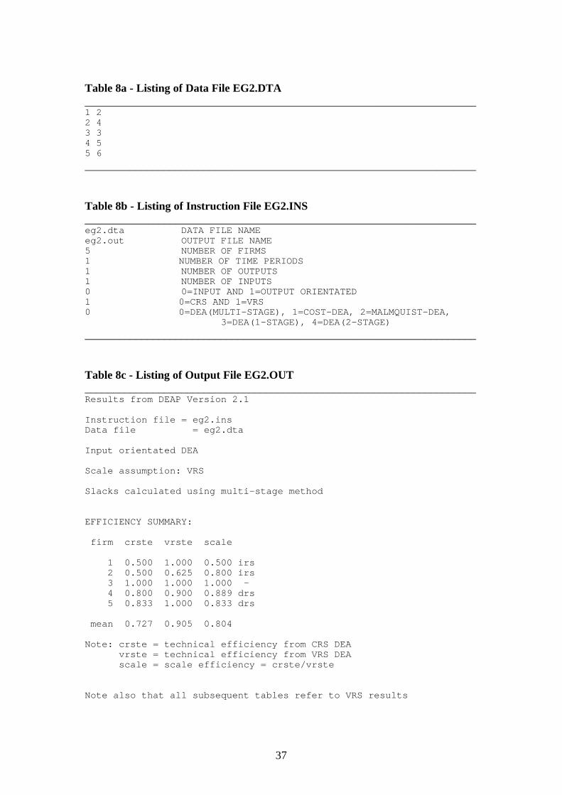
5.2 Example 2: An Input-orientated VRS DEA Example

The text file EG2.DTA (refer to Table 8a) contains five observations on one output

and one input. The output is listed in the first column and the input in the second

column. This data is identical to that listed in Table 3.

The EG2.INS file is listed in Table 8b. The only changes relative to EG1.INS is that:

• the input and output file names are different;

• the number of inputs is reduced to 1; and

• there is a “1” entered on the 2nd last line to indicate that VRS is required.

The output file EG1.OUT is reproduced in Table 8c. These results are identical to

those presented in Table 4.

37

Table 8a - Listing of Data File EG2.DTA_____________________________________________________________________1 22 43 34 55 6

_____________________________________________________________________



_____________________________________________________________________



Input orientated DEA

Scale assumption: VRS

Slacks calculated using multi-stage method

EFFICIENCY SUMMARY:

firm crste vrste scale

1 0.500 1.000 0.500 irs 2 0.500 0.625 0.800 irs 3 1.000 1.000 1.000 - 4 0.800 0.900 0.889 drs 5 0.833 1.000 0.833 drs

mean 0.727 0.905 0.804

Note: crste = technical efficiency from CRS DEA vrste = technical efficiency from VRS DEA scale = scale efficiency = crste/vrste

Note also that all subsequent tables refer to VRS results

38

SUMMARY OF OUTPUT SLACKS:

firm output: 1 1 0.000 2 0.000 3 0.000 4 0.000 5 0.000

mean 0.000

SUMMARY OF INPUT SLACKS:

firm input: 1 1 0.000 2 0.000 3 0.000 4 0.000 5 0.000

mean 0.000

SUMMARY OF PEERS:

firm peers: 1 1 2 1 3 3 3 4 3 5 5 5

SUMMARY OF PEER WEIGHTS: (in same order as above)

firm peer weights: 1 1.000 2 0.500 0.500 3 1.000 4 0.500 0.500 5 1.000

PEER COUNT SUMMARY: (i.e., no. times each firm is a peer for another)

firm peer count: 1 1 2 0 3 2 4 0 5 1

SUMMARY OF OUTPUT TARGETS:

firm output: 1 1 1.000 2 2.000 3 3.000 4 4.000

39

5 5.000

SUMMARY OF INPUT TARGETS:

firm input: 1 1 2.000 2 2.500 3 3.000 4 4.500 5 6.000

FIRM BY FIRM RESULTS:

Results for firm: 1Technical efficiency = 1.000Scale efficiency = 0.500 (irs)PROJECTION SUMMARY: variable original radial slack projected value movement movement value output 1 1.000 0.000 0.000 1.000 input 1 2.000 0.000 0.000 2.000LISTING OF PEERS: peer lambda weight 1 1.000

Results for firm: 2Technical efficiency = 0.625Scale efficiency = 0.800 (irs)PROJECTION SUMMARY: variable original radial slack projected value movement movement value output 1 2.000 0.000 0.000 2.000 input 1 4.000 -1.500 0.000 2.500LISTING OF PEERS: peer lambda weight 1 0.500 3 0.500

Results for firm: 3Technical efficiency = 1.000Scale efficiency = 1.000 (crs)PROJECTION SUMMARY: variable original radial slack projected value movement movement value output 1 3.000 0.000 0.000 3.000 input 1 3.000 0.000 0.000 3.000LISTING OF PEERS: peer lambda weight 3 1.000

Results for firm: 4Technical efficiency = 0.900Scale efficiency = 0.889 (drs)PROJECTION SUMMARY: variable original radial slack projected value movement movement value output 1 4.000 0.000 0.000 4.000

40

input 1 5.000 -0.500 0.000 4.500LISTING OF PEERS: peer lambda weight 3 0.500 5 0.500

Results for firm: 5Technical efficiency = 1.000Scale efficiency = 0.833 (drs)PROJECTION SUMMARY: variable original radial slack projected value movement movement value output 1 5.000 0.000 0.000 5.000 input 1 6.000 0.000 0.000 6.000LISTING OF PEERS: peer lambda weight 5 1.000

_____________________________________________________________________

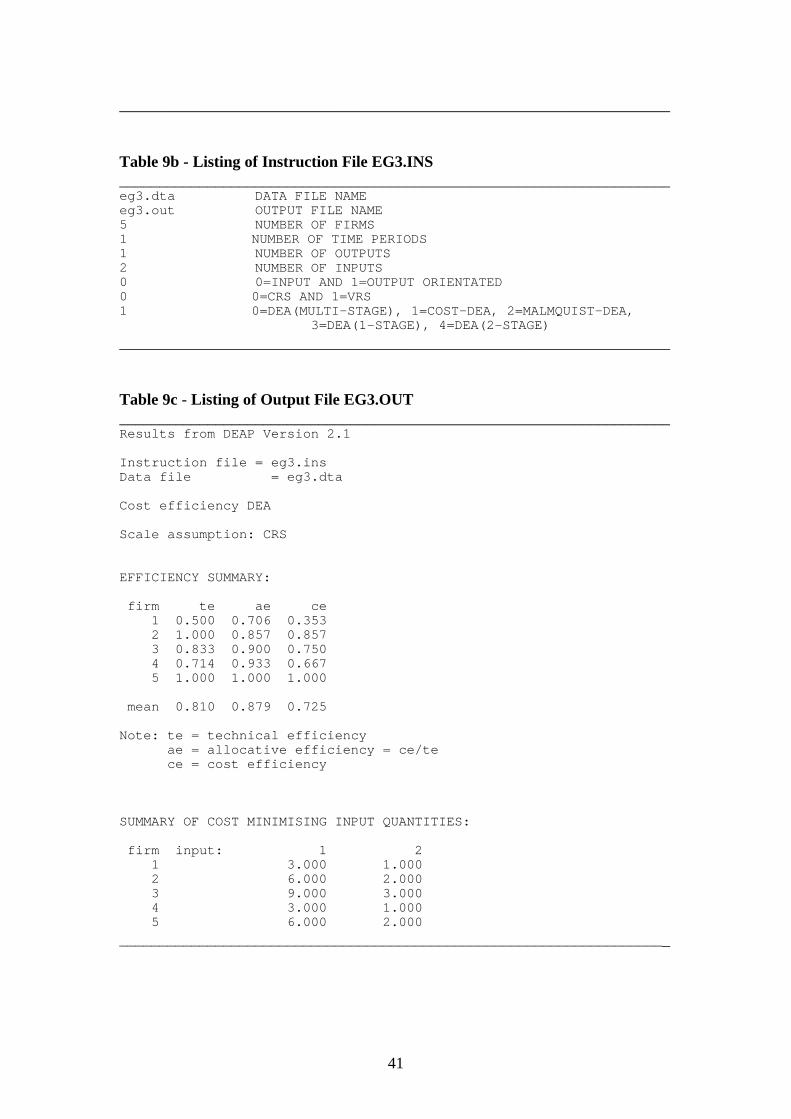
5.3 Example 3: A Cost Efficiency DEA Example

The text file EG3.DTA (refer to Table 9a) contains the same data as EG1.DTA. That

is, five observations on one output and two inputs. The output is listed in the first

column and the inputs in the next two columns. In addition to this, two columns

containing input price data are listed to the right of these. In this particular example

we assume all firms face the same prices and that these prices are 1 and 3 for inputs 1

and 2, respectively.



• there is a “1” entered on the last line to indicate that a cost efficiency DEA is

required.

The output file EG3.OUT is reproduced in Table 9c. The results in the efficiencies

summary table are identical to those listed in EG1.OUT with the exception that

allocative and cost efficiencies are now also listed. Furthermore, a table of input

quantities for minimum cost production are now also listed.

Table 9a - Listing of Data File EG3.DTA_____________________________________________________________________1 2 5 1 32 2 4 1 33 6 6 1 31 3 2 1 32 6 2 1 3

41

_____________________________________________________________________



_____________________________________________________________________



Cost efficiency DEA

Scale assumption: CRS

EFFICIENCY SUMMARY:

firm te ae ce 1 0.500 0.706 0.353 2 1.000 0.857 0.857 3 0.833 0.900 0.750 4 0.714 0.933 0.667 5 1.000 1.000 1.000

mean 0.810 0.879 0.725

Note: te = technical efficiency ae = allocative efficiency = ce/te ce = cost efficiency

SUMMARY OF COST MINIMISING INPUT QUANTITIES:

firm input: 1 2 1 3.000 1.000 2 6.000 2.000 3 9.000 3.000 4 3.000 1.000 5 6.000 2.000

_____________________________________________________________________

42

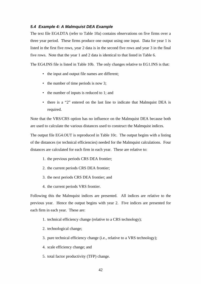
5.4 Example 4: A Malmquist DEA Example

The text file EG4.DTA (refer to Table 10a) contains observations on five firms over a

three year period. These firms produce one output using one input. Data for year 1 is

listed in the first five rows, year 2 data is in the second five rows and year 3 in the final

five rows. Note that the year 1 and 2 data is identical to that listed in Table 6.



• the number of time periods is now 3;

• the number of inputs is reduced to 1; and

• there is a “2” entered on the last line to indicate that Malmquist DEA is

required.

Note that the VRS/CRS option has no influence on the Malmquist DEA because both

are used to calculate the various distances used to construct the Malmquist indices.

The output file EG4.OUT is reproduced in Table 10c. The output begins with a listing

of the distances (or technical efficiencies) needed for the Malmquist calculations. Four

distances are calculated for each firm in each year. These are relative to:

1. the previous periods CRS DEA frontier;

2. the current periods CRS DEA frontier;

3. the next periods CRS DEA frontier; and

4. the current periods VRS frontier.

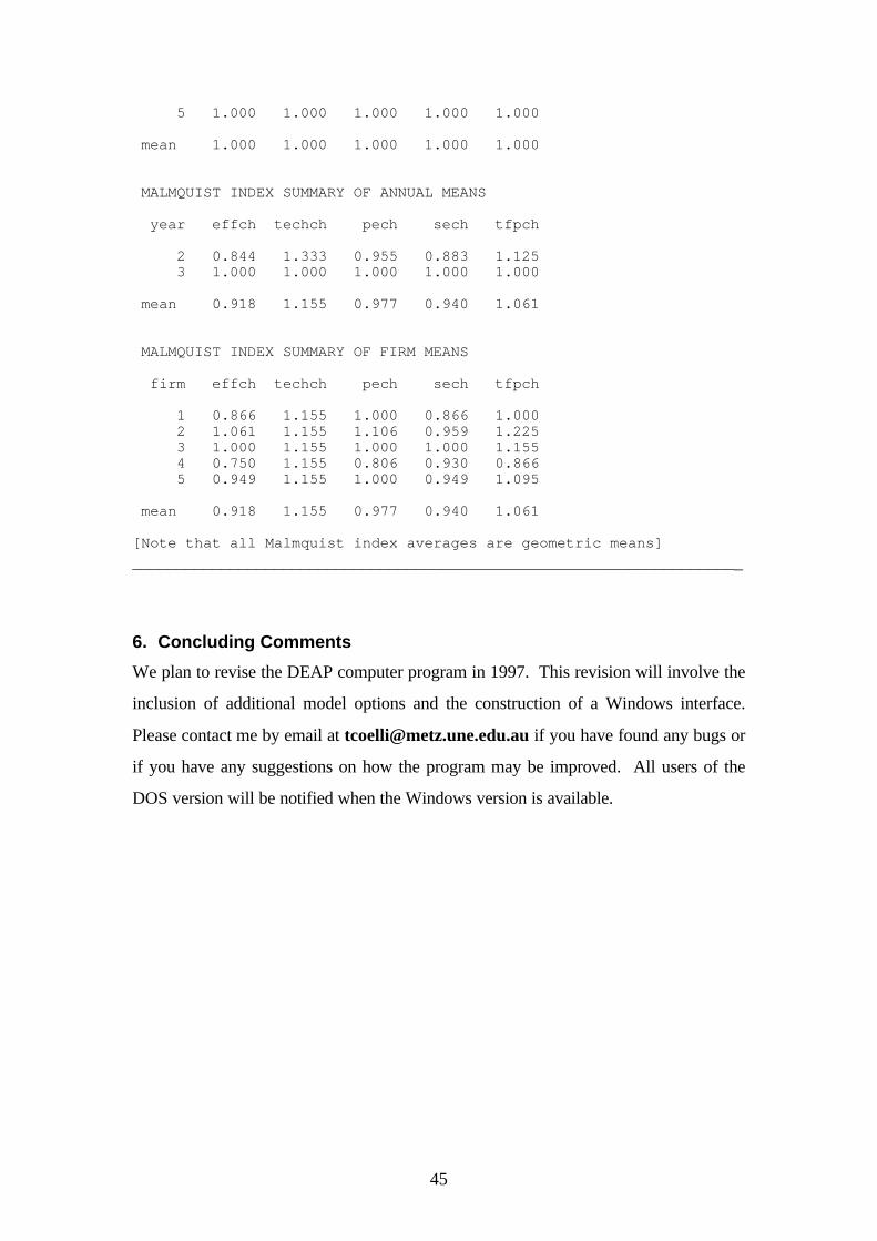
Following this the Malmquist indices are presented. All indices are relative to the

previous year. Hence the output begins with year 2. Five indices are presented for

each firm in each year. These are:

1. technical efficiency change (relative to a CRS technology);

2. technological change;

3. pure technical efficiency change (i.e., relative to a VRS technology);

4. scale efficiency change; and

5. total factor productivity (TFP) change.

43

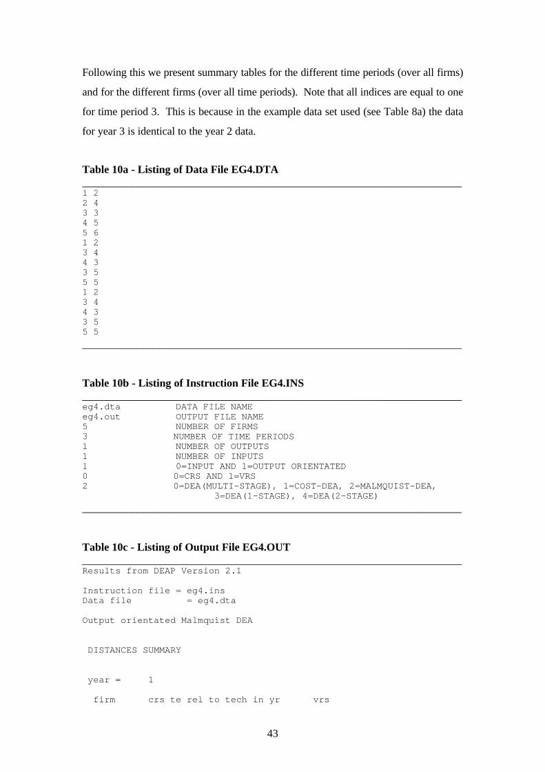
Following this we present summary tables for the different time periods (over all firms)

and for the different firms (over all time periods). Note that all indices are equal to one

for time period 3. This is because in the example data set used (see Table 8a) the data

for year 3 is identical to the year 2 data.

Table 10a - Listing of Data File EG4.DTA_____________________________________________________________________1 22 43 34 55 61 23 44 33 55 51 23 44 33 55 5

_____________________________________________________________________



_____________________________________________________________________



Output orientated Malmquist DEA

DISTANCES SUMMARY

year = 1

firm crs te rel to tech in yr vrs

44

no. ************************ te t-1 t t+1

1 0.000 0.500 0.375 1.000 2 0.000 0.500 0.375 0.545 3 0.000 1.000 0.750 1.000 4 0.000 0.800 0.600 0.923 5 0.000 0.833 0.625 1.000

mean 0.000 0.727 0.545 0.894

year = 2

firm crs te rel to tech in yr vrs no. ************************ te t-1 t t+1

1 0.500 0.375 0.375 1.000 2 0.750 0.563 0.563 0.667 3 1.333 1.000 1.000 1.000 4 0.600 0.450 0.450 0.600 5 1.000 0.750 0.750 1.000

mean 0.837 0.628 0.628 0.853

year = 3

firm crs te rel to tech in yr vrs no. ************************ te t-1 t t+1

1 0.375 0.375 0.000 1.000 2 0.563 0.563 0.000 0.667 3 1.000 1.000 0.000 1.000 4 0.450 0.450 0.000 0.600 5 0.750 0.750 0.000 1.000

mean 0.628 0.628 0.000 0.853

[Note that t-1 in year 1 and t+1 in the final year are not defined]

MALMQUIST INDEX SUMMARY

year = 2

firm effch techch pech sech tfpch

1 0.750 1.333 1.000 0.750 1.000 2 1.125 1.333 1.222 0.920 1.500 3 1.000 1.333 1.000 1.000 1.333 4 0.562 1.333 0.650 0.865 0.750 5 0.900 1.333 1.000 0.900 1.200

mean 0.844 1.333 0.955 0.883 1.125

year = 3


1 1.000 1.000 1.000 1.000 1.000 2 1.000 1.000 1.000 1.000 1.000 3 1.000 1.000 1.000 1.000 1.000 4 1.000 1.000 1.000 1.000 1.000

45

5 1.000 1.000 1.000 1.000 1.000

mean 1.000 1.000 1.000 1.000 1.000

MALMQUIST INDEX SUMMARY OF ANNUAL MEANS

year effch techch pech sech tfpch

2 0.844 1.333 0.955 0.883 1.125 3 1.000 1.000 1.000 1.000 1.000

mean 0.918 1.155 0.977 0.940 1.061

MALMQUIST INDEX SUMMARY OF FIRM MEANS


1 0.866 1.155 1.000 0.866 1.000 2 1.061 1.155 1.106 0.959 1.225 3 1.000 1.155 1.000 1.000 1.155 4 0.750 1.155 0.806 0.930 0.866 5 0.949 1.155 1.000 0.949 1.095

mean 0.918 1.155 0.977 0.940 1.061

[Note that all Malmquist index averages are geometric means]

_____________________________________________________________________

6. Concluding Comments

We plan to revise the DEAP computer program in 1997. This revision will involve the

inclusion of additional model options and the construction of a Windows interface.

Please contact me by email at [email protected] if you have found any bugs or

if you have any suggestions on how the program may be improved. All users of the

DOS version will be notified when the Windows version is available.

46

REFERENCES

Afriat, S.N. (1972), “Efficiency Estimation of Production Functions”, InternationalEconomic Review, 13, 568-598.

Ali, A.I. and L.M. Seiford (1993), “The Mathematical Programming Approach toEfficiency Analysis”, in Fried, H.O., C.A.K. Lovell and S.S. Schmidt (Eds),The Measurement of Productive Efficiency, Oxford University Press, NewYork, 120-159.

Banker, R.D., Charnes, A. and Cooper, W.W. (1984), “Some Models for EstimatingTechnical and Scale Inefficiencies in Data Envelopment Analysis”,Management Science, 30, 1078-1092.

BIE (1994), International Performance Indicators: Aviation, research report #59,BIE, Canberra.

Boles, J.N. (1966), “Efficiency Squared - Efficient Computation of EfficiencyProceedings of the 39th Annual Meeting of the Western Farm

Economic Association, pp 137-142.

Charnes, A., W.W. Cooper, A.Y. Lewin and L.M. Seiford (1995), “Data EnvelopmentAnalysis: Theory, Methodology and Applications”, Kluwer.

Charnes, A., W.W. Cooper and E. Rhodes (1978), “Measuring the Efficiency ofEuropean Journal of Operations Research, 2, 429-

444.

Charnes, A., W.W. Cooper, J. Rousseau and J.

Report CCS 558, Centre for Cybernetic Studies, The University of Texas atAustin.

Coelli, T.J. (1992), “A Computer Program for Frontier Production FunctionEstimation: FRONTIER, Version 2.0”, Economics Letters, 39, 29-32.

Coelli, T.J. (1994), A Guide to FRONTIER Version 4.1: A Computer Program forStochastic Frontier Production and Cost Function Estimation, mimeo,Department of Econometrics, University of New England, Armidale.

Coelli, T.J. (1997), A Multi-Stage Methodology for the Solution of Orientated DEAModels, mimeo, Centre for Efficiency and Productivity Analysis, University ofNew England, Armidale.

Coelli, T.J. and S. Perelman (1996), “A Comparison of Parametric and Non-parametricDistance Functions: With Application to European Railways”, CREPPDiscussion Paper, University of Liege, Liege.

Debreu, G. (1951), “The Coefficient of Resource Utilisation”, Econometrica, 19, 273-292.

Fare, R., S. Grosskopf, and C.A.K. Lovell (1985), The Measurement of Efficiency ofProduction, Boston, Kluwer.

Fare, R., S. Grosskopf, and C.A.K. Lovell (1994), Production Frontiers, CambridgeUniversity Press.

Fare, R. and C.A.K. Lovell (1978), “Measuring the Technical Efficiency of

47

Production”, Journal of Economic Theory, 19, 150-162.

Fare, R., S. Grosskopf, M. Norris and Z. Zhang (1994), “Productivity Growth,Technical Progress, and Efficiency Changes in Industrialised Countries”,American Economic Review, 84, 66-83.

Farrell, M.J. (1957), “The Measurement of Productive Efficiency”, Journal of theRoyal Statistical Society, A CXX, Part 3, 253-290.

Ferrier, G.D. and C.A.K. Lovell (1990), “Measuring Cost Efficiency in Banking:Econometric and Linear Programming Evidence”, Journal of Econometrics,46, 229-245.

Ganley, J.A and J.S. Cubbin (1992), Public Sector Efficiency Measurement:Applications of Data Envelopment Analysis, North Holland, Amsterdam.

Grosskopf, S. (1993), “Efficiency and Productivity”, in Fried, H.O., C.A.K. Lovell andS.S. Schmidt (Eds), The Measurement of Productive Efficiency, OxfordUniversity Press, New York, 160-194.

Koopmans, T.C. (1951), “An Analysis of Production as an Efficient Combination ofKoopmans, Ed., Activity Analysis of Production and

Allocation, Cowles Commission for Research in Economics, Monograph No.13, Wiley, New York.

Lovell, C.A.K. (1993), “Production Frontiers and Productive Efficiency”, in Fried,H.O., C.A.K. Lovell and S.S. Schmidt (Eds), The Measurement of ProductiveEfficiency, Oxford University Press, New York, 3-67.

Lovell, C.A.K. (1994), “Linear Programming Approaches to the Measurement andAnalysis of Productive Efficiency”, Top, 2, 175-248.

Norman, M. and B. Stoker (1991), Data Envelopment Analysis: An Assessment ofPerformance, Wiley.

Shepherd, R.W. (1970), Theory of Cost and Production Functions, Princeton,Princeton University Press.

Seiford, L.M. (1996), “Data Envelopment Analysis: The Evolution of the State of theArt (1978-1995)”, Journal of Productivity Analysis, 7, 99-138.

Seiford, L.M. and R.M. Thrall (1990), “Recent Developments in DEA: TheMathematical Approach to Frontier Analysis”, Journal of Econometrics, 46, 7-38.

48

APPENDIX

This appendix simply provides a collection of technical and semi-technical pointsregarding the DEAP computer program.

• Computer requirements: The program is written for an IBM compatible computer.A minimum configuration would be a 386 with a math-coprocessor and 4 MB RAMrunning DOS 5.0 and/or Windows 3.1 (or higher).

• Size limits: The program has been written using dynamic array allocations so thesize of the DEA problem that can be handled is essentially only limited by thememory you have available on your computer. The only limits which may comeinto play relate to the listing of information on slacks and peers where the outputtables are limited to 99 columns (I am yet to see a DEA analysis with dimensionswhich get even half way to these limits). It should also be noted that the slacks arereported in fixed-width fields. Hence if a slack value is larger than 108 it will not bereported and a string of stars (************) will appear instead. This can beavoided by scaling your data prior to estimating the DEA problem. For example, ifcoal input in an analysis of power station efficiency is expressed in tonnes, you maychoose to change the units of measurement to thousand or million tonne units.

• Scaling: The program scales all quantity data by dividing by the sample meansbefore running the DEA. The slack information is then scaled back to original unitsbefore it is reported.

• The technical efficiency estimates reported in output orientated models are invertedso they vary between 0 and 1.

• All program files and data, instruction and output files must be stored in the samedirectory. The program is not able to access files in directories other than thedirectory that the program resides in.

• The program can sometimes report that “no solutions satisfy the constraints given”.This can often be corrected by editing the DEAP.000 file and increasing the size ofthe EPS parameter.

• The program can also occasionally cycle indefinitely (i.e., run for more than 5minutes). To stop the program running press ctrl/c. Then to avoid this problemone can also try increasing the size of the EPS parameter. Also note that cyclingwill often occur if you have zeros in your data and you use the multi-stage DEAmethod.

• For further information on other CEPA software and publications, refer to theCEPA web site: http://www.une.edu.au/econometrics/cepa.htm

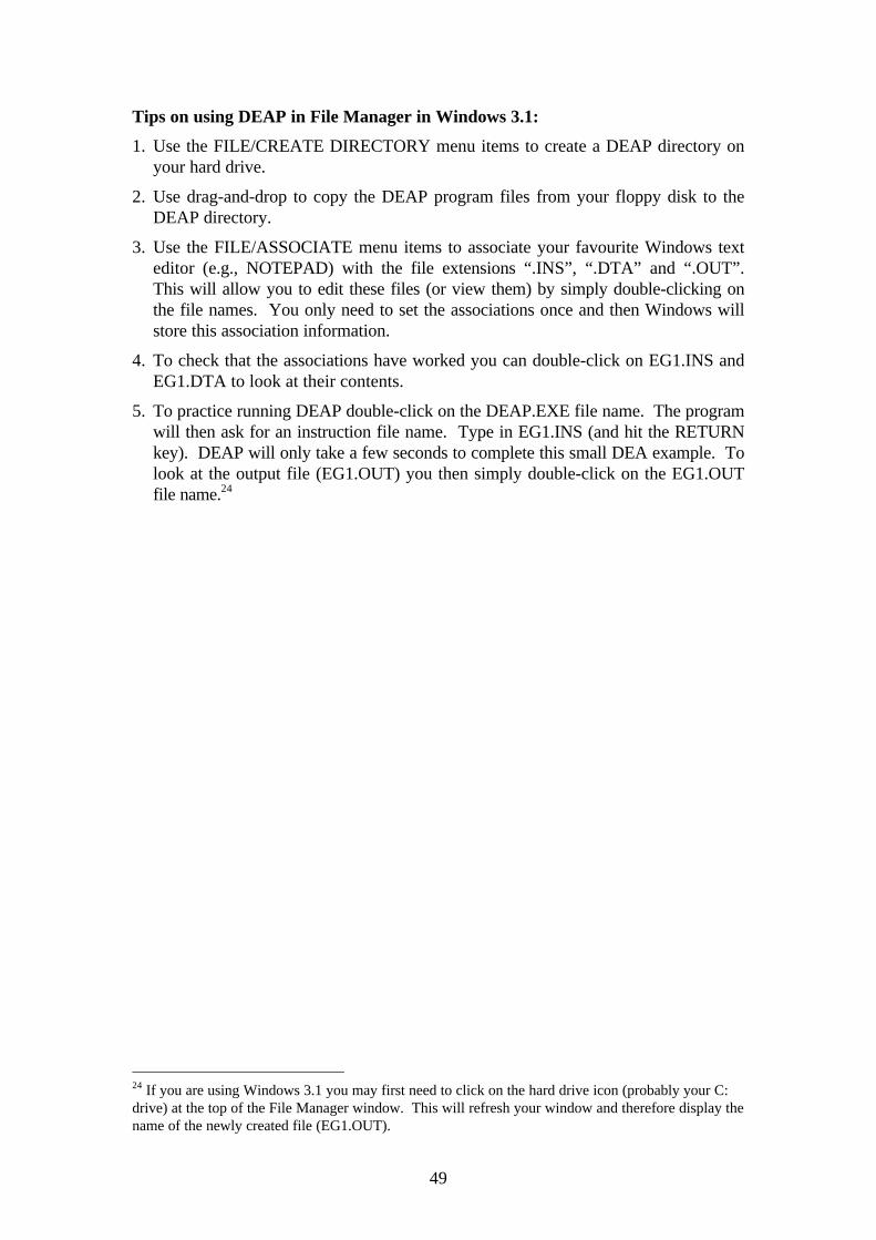
49

Tips on using DEAP in File Manager in Windows 3.1:

1. Use the FILE/CREATE DIRECTORY menu items to create a DEAP directory onyour hard drive.

2. Use drag-and-drop to copy the DEAP program files from your floppy disk to theDEAP directory.

3. Use the FILE/ASSOCIATE menu items to associate your favourite Windows texteditor (e.g., NOTEPAD) with the file extensions “.INS”, “.DTA” and “.OUT”.This will allow you to edit these files (or view them) by simply double-clicking onthe file names. You only need to set the associations once and then Windows willstore this association information.

4. To check that the associations have worked you can double-click on EG1.INS andEG1.DTA to look at their contents.

5. To practice running DEAP double-click on the DEAP.EXE file name. The programwill then ask for an instruction file name. Type in EG1.INS (and hit the RETURNkey). DEAP will only take a few seconds to complete this small DEA example. Tolook at the output file (EG1.OUT) you then simply double-click on the EG1.OUTfile name.24

24 If you are using Windows 3.1 you may first need to click on the hard drive icon (probably your C:drive) at the top of the File Manager window. This will refresh your window and therefore display thename of the newly created file (EG1.OUT).

A Guide to DEAP Version 2.1: A Data Envelopment Analysis (Computer

Documents

Transcript of A Guide to DEAP Version 2.1: A Data Envelopment Analysis (Computer