A Green Integrated Inventory Model for a Three-Tier Supply ...
14
Engineering International, Volume 8, No. 2 (2020) ISSN 2409-3629 Asian Business Consortium | EI Page 73 A Green Integrated Inventory Model for a Three-Tier Supply Chain of an Agricultural Product S. M. Shahidul Islam * , Risat Hossain, Mst. Jamila Yasmin Department of Mathematics, Hajee Mohammad Danesh Science and Technology University, Dinajpur-5200, BANGLADESH * Corresponding Contact: Email: [email protected] ABSTRACT Green supply chain management coordinates environment issues into the supply chain business. It has been popular to both academicians and practitioners. Smooth supply of processed agricultural products is essential for human beings and pets. In some models, excess raw materials, byproducts and defected products are kept neglected in producing and marketing finished products. Here, we have presented a three-tier green supply chain model for an agricultural product where byproducts are used for some purposes. Solution procedure of the model is derived. We have demonstrated the model using two numerical example problems. Key words: Agricultural product, green supply chain, integrated inventory, lot size, supply chain, byproduct INTRODUCTION Controlling of environmental pollution is a burning issue in the universe. Usually, a green supply chain (SC) uses the mechanism to reduce environmental pollution during its functioning. So, the topic has got the attention of researchers worldwide. We are also interested of modeling a green supply chain problem with coordinated inventory policy. Current competitive market imposes companies to integrate with their upstream and downstream players for establishing an improved SC to minimize the management cost. They all supply finished products to customers with reasonable prices (e.g., Gunasekaran et al. 2008; Ben-Daya and Al-Nassar 2008; Moncayo-Martı ´nez and Zhang 2013; Islam and Hoque 2014a; Hellion et al. 2015; Islam and Hoque 2018). Modeling on integrated cost minimization using joint economic lot sizing (JELS) policy has received 12/15/2020 Source of Support: None, No Conflict of Interest: Declared This article is licensed under a Creative Commons Attribution-NonCommercial 4.0 International License. Attribution-NonCommercial (CC BY-NC) license lets others remix, tweak, and build upon work non-commercially, and although the new works must also acknowledge & be non-commercial.
Transcript of A Green Integrated Inventory Model for a Three-Tier Supply ...
Engineering International, Volume 8, No. 2 (2020) ISSN 2409-3629
Asian Business Consortium | EI Page 73
A Green Integrated Inventory Model for a
Three-Tier Supply Chain of an Agricultural
Product S. M. Shahidul Islam*, Risat Hossain, Mst. Jamila Yasmin
Department of Mathematics, Hajee Mohammad Danesh Science and Technology University, Dinajpur-5200, BANGLADESH
*Corresponding Contact:
Email: [email protected]
ABSTRACT
Green supply chain management coordinates environment issues into the supply chain business. It has been popular to both academicians and practitioners. Smooth supply of processed agricultural products is essential for human beings and pets. In some models, excess raw materials, byproducts and defected products are kept neglected in producing and marketing finished products. Here, we have presented a three-tier green supply chain model for an agricultural product where byproducts are used for some purposes. Solution procedure of the model is derived. We have demonstrated the model using two numerical example problems.
Key words: Agricultural product, green supply chain, integrated inventory, lot size, supply chain, byproduct
INTRODUCTION
Controlling of environmental pollution is a burning issue in the universe. Usually, a green supply chain (SC) uses the mechanism to reduce environmental pollution during its functioning. So, the topic has got the attention of researchers worldwide. We are also interested of modeling a green supply chain problem with coordinated inventory policy. Current competitive market imposes companies to integrate with their upstream and downstream players for establishing an improved SC to minimize the management cost.
They all supply finished products to customers with reasonable prices (e.g., Gunasekaran et al. 2008; Ben-Daya and Al-Nassar 2008; Moncayo-Martı ´nez and Zhang 2013; Islam and Hoque 2014a; Hellion et al. 2015; Islam and Hoque 2018). Modeling on integrated cost minimization using joint economic lot sizing (JELS) policy has received
12/15/2020 Source of Support: None, No Conflict of Interest: Declared
This article is licensed under a Creative Commons Attribution-NonCommercial 4.0 International License.
Attribution-NonCommercial (CC BY-NC) license lets others remix, tweak, and build upon work non-commercially, and although the new works must also acknowledge & be non-commercial.

Islam et al.: A Green Integrated Inventory Model for a Three-Tier Supply Chain of an Agricultural Product (73-86)
Page 74 Engineering International, Volume 8, No. 2 (2020)
the devotion of the researchers and also the practitioners in SC business (Banerjee 1986; Baboli et al. 2011; Glock 2012; Wang et al. 2015; Sarmah et al. 2006). Most of the studies related to JELS approach are conducted within the context of a two-tier SC consisting of a vendor and a buyer (Kim et al. 2014; Giri and Bardhan 2015; Hariga et al. 2016). In a two stage SC, the manufacturer on receiving an order produces plenty in one setup, and delivers them to the buyers with a number of shipments to minimize the chain wide cost (Lee 2005; Hoque 2011; Sari et al. 2012).
At the initial stage of JELS study, Goyal (1977) proposed a lot sizing policy for two stage production. Then, considering numerous techniques of supply chain synchronization like equal-sized shipments, unequal sized shipments, combination of equal and unequal sized shipments, etc., researchers established JELS policy as a beneficial tool in SC management (Hill 1999; Goyal and Nebebe 2000; Ben-Daya and Hariga 2004; Ben-Daya et al. 2008). Khouja (2003) extended the JELS policy to a three-tier SC for supplying products from a vendor to several customers. Here, the cycle time at each stage was the integer multiple of the cycle time of the adjacent downstream player. Ben-Daya et al. (2013), and Abdelsalam and Elassal (2014) improved that model by considering common cycle time.
However, the setting to process of agricultural products is somewhat different. In case of processing an agricultural product, essential supplying period for the supplier cannot be an integer multiple of the cycle time of the manufacturer or of the retailer(s). Rather it is a fraction of the manufacturer’s cycle time because the period of harvesting an agricultural product is shorter than the retailing period of a finished product (Islam 2014; Islam and Hoque 2014b; Gal et al. 2008; Ca´rdenas-Barro´n 2012; Islam et al. 2017; Ca´rdenas-Barro´n et al. 2012). There is a scarcity of a three-tier model involving agricultural products within the existing literature. Islam and Hoque (2017) developed a three-tier model of processing an agricultural product, considering raw material supplying period for the supplier as a fraction of the manufacturer’s cycle time (retailing period). Here, JELS policy is utilized to minimize the integrated cost of a cycle period for the proposed supply chain.
In integrated production and inventory decision models, players should realize the chain objectives with the coordinated decision process. Coordinated multi-level productions and inventories are addressed well in the literatures of Ben-Daya and Al-Nassar 2008; Chen and Chen 2005; Chung et al. 2008; Jaber and Goyal 2008; Khouja 2003; Munson and Rosenblatt 2001; Sarmah et al. 2006; Islam and Hoque 2019, Islam et al. 2020. Based on a literature review which has been carried out, a few researches are concerned with the whole manufacturing system, that is, they overlook the defected products of the system. We have proposed here a green supply chain model that considers also the byproducts of the system.
To make the model reader friendly, we have organized the paper as follows. Section 2 defines the problem and describes assumptions and notation. Derivation of the mathematical model is given in Section 3, while the solution technique and algorithm are provided in Section 4. The model is analyzed by numerical example problems in Section. 5. Finally, Section 6 concludes by highlighting the study findings, limitations and future research scopes.

Engineering International, Volume 8, No. 2 (2020) ISSN 2409-3629
Asian Business Consortium | EI Page 75
PROBLEM DEFINITION, ASSUMPTIONS AND NOTATION
Figure 1 provides a flowchart of the raw materials, finished products, byproducts of our three-tier whole green manufacturing supply chain.
After getting a supply order, a supplier, within a short harvesting period, supplies raw materials to Manufacturer. Manufacturer produces finished products and delivers them to type 1 retailers to fulfil their orders. The manufacturer also sends byproducts to Type 2 retailer. The model uses targeted products and byproducts and hence, the environment keeps green. To avoid shortage at any stage, we assume that demand rate of the downstream players is less than or equal to production rate of the upstream players. The following notation are used in developing the model.
A Supplier
Collects raw materials for
manufacturer
Manufacturer
Produces finished products for
type-1 retailers and sends
byproducts to type-2 retailer
Type-1
Retailer 1
Sells finished
products to end
customer
Type-2 Retailer
Sells byproducts
Type-1
Retailer 2
Sells finished
products to end
customer
Type-1
Retailer N
Sells finished
products to end
customer
Type-1
Retailer 3
Sells finished
products to end
customer
Raw materials and finished products flow
Byproducts flow
Figure 1: Scenarios of this three-tier supply chain problem

Islam et al.: A Green Integrated Inventory Model for a Three-Tier Supply Chain of an Agricultural Product (73-86)
Page 76 Engineering International, Volume 8, No. 2 (2020)
Notation
𝑃𝑠 collection rate of the supplier.
𝑃𝑚 production rate of the Manufacturer.
𝐶𝑚 conversion rate of raw materials to finished product.
𝑁 number of type 1 retailers.
𝐷𝑟 demand rate incurred by type 1 retailer 𝑟 (𝐷 = ∑ 𝐷𝑟𝑁𝑟 =1 ).
𝐷𝑟2 demand rate incurred by type 2 retailer.
𝐷𝑚 demand rate of the Manufacturer, 𝐷𝑚 =𝐷
𝐶𝑚.
𝑇 cycle time of the retailers, the manufacturer and the supplier.
𝑀1 number of shipments in a cycle received by the Manufacturer.
𝑀2 number of shipments in a cycle received by a type 1 retailer.
𝑀3 number of shipments in a cycle received by a type 2 retailer.
𝐴𝑚 Manufacturer’s production setup cost.
𝑂𝑚 Manufacturer’s raw item ordering cost.
𝑂𝑟 type 1 retailer’s ordering cost.
𝑂𝑟2 type 2 retailer’s ordering cost.
𝑂𝑠 supplier’s raw material order cost.
𝑆𝑚 cost per shipment from the supplier to the Manufacturer.
𝑆𝑟 cost per shipment from Manufacturer to the type 1 retailer 𝑟.
𝑆𝑟2 cost per shipment from Manufacturer to the type 2 retailer.
𝐻𝑠 holding cost per unit time for the supplier.
𝐻𝑚 per unit raw material holding cost for the Manufacturer per unit time.
𝐻𝑓 per unit finished product holding cost for the Manufacturer per unit time.
𝐻𝑏 per unit byproduct holding cost for the Manufacturer per unit time.
𝐻𝑟 per unit holding cost for type 1 retailers per unit time.
𝐻𝑟2 per unit holding cost for the type 2 retailers per unit time.
𝑇𝐶 entire supply chain cost per unit time.
MATHEMATICAL MODEL DEVELOPMENT
Based on the situation described above, and with the underpinning, assumptions and notation, we formulate the cost components of all players involved in the supply chain. The integrated model of the described problem is presented below.
Type-1 retailers experience only the cost of order (𝑂𝑟/𝑇), transportation (𝑀2𝑆𝑟/𝑇) and holding (𝐻𝑟𝑇𝐷𝑟/2𝑀2). Thus, the total cost per unit time for Type-1 retailers is
𝑇𝐶1 = ∑ (𝑂𝑟
𝑇+
𝑀2𝑆𝑟
𝑇+ 𝐻𝑟
𝑇𝐷𝑟
2𝑀2)𝑁
𝑟=1 . (1)

Engineering International, Volume 8, No. 2 (2020) ISSN 2409-3629
Asian Business Consortium | EI Page 77
As Type-1 retailers, Type-2 retailer incurs the cost of order (𝑂𝑟2/𝑇), transportation (𝑀3𝑆𝑟2
/𝑇)
and byproduct holding (𝐻𝑟2𝑇𝐷𝑟2
/2𝑀3). Therefore, the total cost per unit time for Type-2
retailers is
𝑇𝐶2 =𝑂𝑟2
𝑇+
𝑀3𝑆𝑟2
𝑇+ 𝐻𝑟2
𝑇𝐷𝑟2
2𝑀3 . (2)
Manufacturer bears the cost of raw material, order (𝑂𝑚/𝑇), raw material shipment (𝑀1𝑆𝑚/𝑇),
raw material holding, setup (𝐴𝑚/𝑇), finished product and byproduct holding. (𝑇𝐷𝑚
𝑀1−
𝑇𝐷𝑚𝑃𝑚
𝑀1𝑃𝑠𝐶𝑚)
units of raw material are accumulated to the manufacturer from each shipment, which is depicted in the diagram of ‘Manufacturer’s raw material inventory’ in Figure 2. After 𝑀1-th shipment, raw material inventory gradually decreases to zero in producing finished products. Thus, the raw material inventory (𝑅𝐼𝑚) per unit time is as given below.
𝑅𝐼𝑚 =1
𝑇[
1
2
𝑇𝐷𝑚
𝑀1𝑃𝑠 .
𝑇𝐷𝑚𝑃𝑚
𝑀1𝑃𝑠𝐶𝑚× (𝑀1 − 1) +
1
2{(𝑀1 − 1) (
𝑇𝐷𝑚
𝑀1−
𝑇𝐷𝑚𝑃𝑚
𝑀1𝑃𝑠𝐶𝑚) +
𝑇𝐷𝑚
𝑀1} . {
𝑇𝐷𝑚
𝑃𝑚−
(𝑀1 − 1)𝑇𝐷𝑚
𝑀1𝑃𝑠} +
𝑇𝐷𝑚
𝑀1𝑃𝑠(
𝑇𝐷𝑚
𝑀1 −
𝑇𝐷𝑚𝑃𝑚
𝑀1𝑃𝑠𝐶𝑚 ) {1 + 2 + 3 + ⋯ + (𝑀1 − 1)}],
𝑅𝐼𝑚 =𝑇𝐷𝑚
2
2(
1
𝑃𝑚+
1
𝑀1𝑃𝑠−
1
𝐶𝑚𝑃𝑠).
Therefore, the raw material holding cost (𝐻𝐶𝑚) per unit time for the manufacturer is
−𝐷 𝑃𝑚 − 𝐷
𝑇𝐷2
𝑀2𝑃𝑚
𝑇𝐷
𝑀2𝑃𝑚
𝑇𝐷𝑚
𝑀1
𝑇𝐷𝑚
𝑃𝑠
𝑇𝐷𝑚𝑃𝑚
𝑀1𝑃𝑠𝐶𝑚
Manufacturer’s finished
product inventory
Manufacturer’s raw material
inventory, 𝑀1 = 3
Time
Inventory
𝑇𝐷
𝑃𝑚
Figure 2: On-hand inventories of the manufacturer

Islam et al.: A Green Integrated Inventory Model for a Three-Tier Supply Chain of an Agricultural Product (73-86)
Page 78 Engineering International, Volume 8, No. 2 (2020)
𝐻𝐶𝑚 = 𝐻𝑚𝑇𝐷𝑚
2
2(
1
𝑃𝑚+
1
𝑀1𝑃𝑠−
1
𝐶𝑚𝑃𝑠) (3)
The system inventory (inventories of manufacturer and retailers) of finished product is depicted by the dashed line in ‘Manufacturer’s finished product inventory’ in Figure 2. This inventory increases from 𝑇𝐷2/𝑀2𝑃𝑚 (kept by Type-1 retailers), by the rate of 𝑃𝑚 − 𝐷 during the production period 𝑇𝐷/𝑃𝑚. Then it decreases at a rate of 𝐷 in meeting demand of the retailers up to the end of the cycle. Thus, the average system inventory is
(𝑃𝑚 − 𝐷 )𝑇𝐷
2𝑃𝑚+
𝑇𝐷2
𝑀2𝑃𝑚.
Retailers’ average inventory 𝑇𝐷/2𝑀2 is also included in the average system inventory. Thus, the manufacturer’s finished product inventory holding cost (𝐻𝐶𝑓) per unit time is
𝐻𝐶𝑓 = 𝐻𝑓 [(𝑃𝑚 − 𝐷 )𝑇𝐷
2𝑃𝑚+
𝑇𝐷2
𝑀2𝑃𝑚−
𝑇𝐷
2𝑀2]. (4)
As above, the system inventory of byproduct increases from 𝑇𝐷𝑟2
2
𝑀3(𝐷𝑚−𝐷) (kept by Type-2
retailer), by the rate of (𝐷𝑚 − 𝐷) − 𝐷𝑟2 during the production period
𝑇𝐷𝑟2
(𝐷𝑚−𝐷) or 𝑇𝐷/𝑃𝑚. Then
it decreases at a rate of 𝐷𝑟2 in meeting demand of Type-2 retailer up to the end of the cycle.
Hence, the average system inventory of byproduct is
((𝐷𝑚 − 𝐷) − 𝐷𝑟2 )
𝑇𝐷𝑟2
2(𝐷𝑚−𝐷)+
𝑇𝐷𝑟22
𝑀3(𝐷𝑚−𝐷).
Average inventory (𝑇𝐷𝑟2
2𝑀3) of Type 2 retailer is also included in the average system inventory
above. Thus, the manufacturer’s byproduct inventory holding cost (𝐻𝐶𝑑) per unit time is
𝐻𝐶𝑑 = 𝐻𝑏 [((𝐷𝑚 − 𝐷) − 𝐷𝑟2 )
𝑇𝐷𝑟2
2(𝐷𝑚−𝐷)+
𝑇𝐷𝑟22
𝑀3(𝐷𝑚−𝐷)−
𝑇𝐷𝑟2
2𝑀3].
Hence, the manufacturer’s total cost (𝑇𝐶3) per unit time is given by
𝑇𝐶3 =𝑂𝑚
𝑇+
𝑀1𝑆𝑚
𝑇+
𝐴𝑚
𝑇+ 𝐻𝑚
𝑇𝐷𝑚2
2(
1
𝑃𝑚+
1
𝑀1𝑃𝑠−
1
𝐶𝑚𝑃𝑠) + 𝐻𝑓 [(𝑃𝑚 − 𝐷 )
𝑇𝐷
2𝑃𝑚+
𝑇𝐷2
𝑀2𝑃𝑚−
𝑇𝐷
2𝑀2] +
𝐻𝑏 [((𝐷𝑚 − 𝐷) − 𝐷𝑟2 )
𝑇𝐷𝑟2
2(𝐷𝑚−𝐷)+
𝑇𝐷𝑟22
𝑀3(𝐷𝑚−𝐷)−
𝑇𝐷𝑟2
2𝑀3] (5)
Supplier incurs only the cost of ordering, 𝑂𝑠/𝑇, and holding, 𝐻𝑠𝑇𝐷𝑚2/2𝑀1𝑃𝑠, because the
manufacturer takes 𝑇𝐷𝑚/𝑀1 units of raw material from the supplier in each shipment. So, the total cost incurred by the supplier is
𝑇𝐶4 =𝑂𝑠
𝑇+ 𝐻𝑠
𝑇𝐷𝑚2
2𝑀1𝑃𝑠. (6)
Thus, the total supply chain cost is simply the sum of the costs experienced by Type-1 retailers, Type-2 retailer, manufacturer and supplier. Hence, it is found by adding Equations (1), (2), (5) and (6) as follows.
𝑇𝐶(𝑀1, 𝑀2, 𝑀3) =1
𝑇∑ 𝑂𝑟
𝑁𝑟=1 +
𝑀2
𝑇∑ 𝑆𝑟
𝑁𝑟=1 +
𝑇
2𝑀2∑ 𝐻𝑟𝐷𝑟
𝑁𝑟=1 +
𝑂𝑟2
𝑇+
𝑀3𝑆𝑟2
𝑇+
𝐻𝑟2𝑇𝐷𝑟2
2𝑀3+
𝑂𝑚
𝑇+
𝑀1𝑆𝑚
𝑇+
𝐴𝑚
𝑇+
𝐻𝑚𝑇𝐷𝑚2
2𝑃𝑚+
𝐻𝑚𝑇𝐷𝑚2
2𝑀1𝑃𝑠−
𝐻𝑚𝑇𝐷𝑚2
2𝐶𝑚𝑃𝑠+
𝐻𝑓𝑇𝐷
2−
𝐻𝑓𝑇𝐷2
2𝑃𝑚+
𝐻𝑓𝑇𝐷2
𝑀2𝑃𝑚−
𝐻𝑓𝑇𝐷
2𝑀2+
𝐻𝑏𝑇𝐷𝑟2
2−
𝐻𝑏𝑇𝐷𝑟22
2(𝐷𝑚−𝐷)+
𝐻𝑏𝑇𝐷𝑟22
𝑀3(𝐷𝑚−𝐷)−
𝐻𝑏𝑇𝐷𝑟2
2𝑀3+
𝑂𝑠
𝑇+
𝐻𝑠𝑇𝐷𝑚2
2𝑀1𝑃𝑠 (7)
It is supposed to minimize the total supply chain cost in (7) based on the values of 𝑀1, 𝑀2, 𝑀3.

Engineering International, Volume 8, No. 2 (2020) ISSN 2409-3629
Asian Business Consortium | EI Page 79
DEVELOPMENT OF SOLUTION TECHNIQUE
We have to minimize the integrated cost function (7) with respect to the integer variables𝑀1 , 𝑀2 𝑎𝑛𝑑 𝑀3. The model is solved using the calculus method of optimization. To obtain integer solutions to the variables 𝑀1 , 𝑀2 𝑎𝑛𝑑 𝑀3 for integrated minimal total cost, we use parallel multiple jumps technique as used by (e.g., Abdelsalam and Elassal 2014; Ca´rdenas-Barro´n et al. 2012; Islam and Hoque 2017). We reorganize the total cost function (7) as follows,
𝑇𝐶(𝑀1, 𝑀2, 𝑀3) =1
𝑀1[𝑀1
2 𝑆𝑚
𝑇+ 𝑀1 {
1
𝑀2(𝑀2
2 1
𝑇∑ 𝑆𝑟
𝑁𝑟=1 + 𝑀2 (
1
𝑇∑ 𝑂𝑟
𝑁𝑟=1 +
𝑂𝑚
𝑇+
𝐴𝑚
𝑇+
𝑂𝑠
𝑇+
𝐻𝑚𝑇𝐷𝑚2
2𝑃𝑚+
𝐻𝑓𝑇𝐷
2−
𝐻𝑚𝑇𝐷𝑚2
2𝐶𝑚𝑃𝑠−
𝐻𝑓𝑇𝐷2
2𝑃𝑚) + (
𝑇
2∑ 𝐻𝑟
𝑁𝑟=1 𝐷𝑟 +
𝐻𝑓𝑇𝐷2
𝑃𝑚−
𝐻𝑓𝑇𝐷
2))} + (
𝐻𝑚𝑇𝐷𝑚2
2𝑃𝑠+
𝐻𝑠𝑇𝐷𝑚2
2𝑃𝑠 )] +
1
𝑀3[ 𝑀3
2 𝑆𝑟2
𝑇+ 𝑀3 {
𝑂𝑟2
𝑇+
𝐻𝑏𝑇𝐷𝑟2
2−
𝐻𝑏𝑇𝐷𝑟22
2(𝐷𝑚−𝐷)} + {
𝐻𝑟2𝑇𝐷𝑟2
2+
𝐻𝑏𝑇𝐷𝑟22
(𝐷𝑚−𝐷)−
𝐻𝑏𝑇𝐷𝑟2
2} ]. (8)
Denoting, 𝛾 =𝑆𝑚
𝑇 , 𝛽 =
𝐻𝑚𝑇𝐷𝑚2
2𝑃𝑠+
𝐻𝑠𝑇𝐷𝑚2
2𝑃𝑠 , 𝜃 =
1
𝑇∑ 𝑂𝑟
𝑁𝑟=1 +
𝑂𝑚
𝑇+
𝐴𝑚
𝑇+
𝑂𝑠
𝑇+
𝐻𝑚𝑇𝐷𝑚2
2𝑃𝑚+
𝐻𝑓𝑇𝐷
2−
𝐻𝑚𝑇𝐷𝑚2
2𝐶𝑚𝑃𝑠−
𝐻𝑓𝑇𝐷2
2𝑃𝑚 , 𝜑 =
𝑇
2∑ 𝐻𝑟
𝑁𝑟=1 𝐷𝑟 +
𝐻𝑓𝑇𝐷2
𝑃𝑚−
𝐻𝑓𝑇𝐷
2, 휀 =
1
𝑇∑ 𝑆𝑟
𝑁𝑟=1 , 𝜎 =
𝑂𝑟2
𝑇+
𝐻𝑏𝑇𝐷𝑟2
2−
𝐻𝑏𝑇𝐷𝑟22
2(𝐷𝑚−𝐷), 𝜇 =
𝐻𝑟2𝑇𝐷𝑟2
2+
𝐻𝑏𝑇𝐷𝑟22
(𝐷𝑚−𝐷)−
𝐻𝑏𝑇𝐷𝑟2
2, 𝛿 =
𝑆𝑟2
𝑇, we have,
𝑇𝐶(𝑀1, 𝑀2, 𝑀3) =1
𝑀1[𝑀1
2𝛾 + 𝑀1 {1
𝑀2(𝑀2
2휀 + 𝑀2𝜃 + 𝜑)} + 𝛽] +1
𝑀3[(𝑀3
2𝛿 + 𝑀3𝜎) + 𝜇]. (9)
Considering the necessary condition, 𝜕
𝜕𝑀1(𝑇𝐶) = 0,
𝜕
𝜕𝑀2(𝑇𝐶) = 0 and
𝜕
𝜕𝑀3(𝑇𝐶) = 0 for
minimization of 𝑇𝐶(𝑀1, 𝑀2, 𝑀3) in (9), and hence we have
𝑀1 = √𝐷𝑚
2 𝑇2(𝐻𝑚+𝐻𝑠)
2𝑃𝑠𝑆𝑚= √
𝛽
𝛾 , (10)
𝑀2 = √𝑇
∑ 𝑆𝑟𝑁𝑟=1
(𝑇 ∑ 𝐻𝑟𝐷𝑟
𝑁𝑟=1
2+
𝐻𝑓𝑇𝐷2
𝑃𝑚−
𝐻𝑓𝑇𝐷
2) = √
𝜑 , (11)
𝑀3 = √𝑇
𝑆𝑟2
(𝐻𝑟2𝑇𝐷𝑟2
2−
𝐻𝑏𝑇𝐷𝑟2
2+
𝐻𝑏𝑇𝐷𝑟22
𝐷𝑚−𝐷) = √
𝜇
𝛿 . (12)
The critical values in Equations (10), (11) and (12) are the optimal values of 𝑀1 , 𝑀2 𝑎𝑛𝑑 𝑀3 respectively because
𝜕2
𝜕𝑀12
(𝑇𝐶) =𝐻𝑚𝑇𝐷𝑚
2
𝑀13𝑃𝑠
+𝐻𝑠𝑇𝐷𝑚
2
𝑀13𝑃𝑠
> 0,
𝜕2
𝜕𝑀12 (𝑇𝐶)
𝜕2
𝜕𝑀22 (𝑇𝐶) −
𝜕2
𝜕𝑀1𝜕𝑀2(𝑇𝐶)
𝜕2
𝜕𝑀2𝜕𝑀1(𝑇𝐶) = (
𝐻𝑚𝑇𝐷𝑚2
𝑀13𝑃𝑠
+𝐻𝑠𝑇𝐷𝑚
2
𝑀13𝑃𝑠
) (𝑇
𝑀23 ∑ 𝐻𝑟𝐷𝑟
𝑁𝑟=1 +
2𝐻𝑓𝑇𝐷2
𝑀23𝑃𝑚
−
𝐻𝑓𝑇𝐷
𝑀23 ) > 0,
and
𝜕2
𝜕𝑀12 (𝑇𝐶)
𝜕2
𝜕𝑀22 (𝑇𝐶)
𝜕2
𝜕𝑀32 (𝑇𝐶) −
𝜕2
𝜕𝑀12 (𝑇𝐶)
𝜕2
𝜕𝑀2𝜕𝑀3(𝑇𝐶)
𝜕2
𝜕𝑀3𝜕𝑀2(𝑇𝐶) = (
𝐻𝑚𝑇𝐷𝑚2
𝑀13𝑃𝑠
+
𝐻𝑠𝑇𝐷𝑚2
𝑀13𝑃𝑠
) (𝑇
𝑀23 ∑ 𝐻𝑟𝐷𝑟
𝑁𝑟=1 +
2𝐻𝑓𝑇𝐷2
𝑀23𝑃𝑚
−𝐻𝑓𝑇𝐷
𝑀23 ) (
2𝐻𝑏𝑇𝐷𝑟22
𝑀33(𝐷𝑚−𝐷)
−𝐻𝑏𝑇𝐷𝑟2
𝑀33 +
𝐻𝑟2𝑇𝐷𝑟2
𝑀33 ) > 0.
Islam et al.: A Green Integrated Inventory Model for a Three-Tier Supply Chain of an Agricultural Product (73-86)
Page 80 Engineering International, Volume 8, No. 2 (2020)
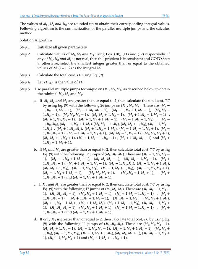
The values of 𝑀1 , 𝑀2 𝑎𝑛𝑑 𝑀3 are rounded up to obtain their corresponding integral values. Following algorithm is the summarization of the parallel multiple jumps and the calculus method.
Solution Algorithm
Step 1 Initialize all given parameters.
Step 2 Calculate values of 𝑀1, 𝑀2 𝑎𝑛𝑑 𝑀3 using Eqs. (10), (11) and (12) respectively. If any of 𝑀1, 𝑀2 𝑎𝑛𝑑 𝑀3 is not real, then this problem is inconsistent and GOTO Step 8; otherwise, select the smallest integer greater than or equal to the obtained values of Mi (i = 1, 2) as the integral Mi.
Step 3 Calculate the total cost, 𝑇𝐶 using Eq. (9).
Step 4 Let 𝑇𝐶 𝑜𝑙𝑑 is the value of 𝑇𝐶.
Step 5 Use parallel multiple jumps technique on (𝑀1, 𝑀2, 𝑀3) as described below to obtain the minimal 𝑀1, 𝑀2 and 𝑀3.
a. If 𝑀1, 𝑀2 𝑎𝑛𝑑 𝑀3 are greater than or equal to 2, then calculate the total cost, 𝑇𝐶 by using Eq. (9) with the following 26 jumps on (𝑀1, 𝑀2, 𝑀3). These are (𝑀1 −1, 𝑀2 − 1, 𝑀3 − 1), (𝑀1 − 1, 𝑀2, 𝑀3 − 1), (𝑀1 − 1, 𝑀2 + 1, 𝑀3 − 1), (𝑀1, 𝑀2 −1, 𝑀3 − 1), (𝑀1, 𝑀2, 𝑀3 − 1), (𝑀1, 𝑀2 + 1, 𝑀3 − 1), (𝑀1 + 1, 𝑀2 − 1, 𝑀3 − 1) , (𝑀1 + 1, 𝑀2, 𝑀3 − 1), (𝑀1 + 1, 𝑀2 + 1, 𝑀3 − 1), (𝑀1 − 1, 𝑀2 − 1, 𝑀3) , (𝑀1 −1, 𝑀2, 𝑀3), (𝑀1 − 1, 𝑀2 + 1, 𝑀3), (𝑀1, 𝑀2 − 1, 𝑀3), (𝑀1, 𝑀2 + 1, 𝑀3), (𝑀1 + 1, 𝑀2 −
1, 𝑀3) , (𝑀1 + 1, 𝑀2, 𝑀3), (𝑀1 + 1, 𝑀2 + 1, 𝑀3), (𝑀1 − 1, 𝑀2 − 1, 𝑀3 + 1), (𝑀1 −1, 𝑀2, 𝑀3 + 1), (𝑀1 − 1, 𝑀2 + 1, 𝑀3 + 1), (𝑀1, 𝑀2 − 1, 𝑀3 + 1), (𝑀1, 𝑀2, 𝑀3 + 1), (𝑀1, 𝑀2 + 1, 𝑀3 + 1), (𝑀1 + 1, 𝑀2 − 1, 𝑀3 + 1) , (𝑀1 + 1, 𝑀2, 𝑀3 + 1) and (𝑀1 +1, 𝑀2 + 1, 𝑀3 + 1).
b. If 𝑀3 𝑎𝑛𝑑 𝑀1 are greater than or equal to 2, then calculate total cost, 𝑇𝐶 by using Eq. (9) with the following 17 jumps of (𝑀1, 𝑀2, 𝑀3). These are (𝑀1 − 1, 𝑀2, 𝑀3 −1), (𝑀1 − 1, 𝑀2 + 1, 𝑀3 − 1), (𝑀1, 𝑀2, 𝑀3 − 1), (𝑀1, 𝑀2 + 1, 𝑀3 − 1), (𝑀1 +1, 𝑀2, 𝑀3 − 1), (𝑀1 + 1, 𝑀2 + 1, 𝑀3 − 1), (𝑀1 − 1, 𝑀2, 𝑀3), (𝑀1 − 1, 𝑀2 + 1, 𝑀3), (𝑀1, 𝑀2 + 1, 𝑀3), (𝑀1 + 1, 𝑀2, 𝑀3), (𝑀1 + 1, 𝑀2 + 1, 𝑀3), (𝑀1 − 1, 𝑀2, 𝑀3 + 1), (𝑀1 − 1, 𝑀2 + 1, 𝑀3 + 1), (𝑀1, 𝑀2, 𝑀3 + 1), (𝑀1, 𝑀2 + 1, 𝑀3 + 1), (𝑀1 +1, 𝑀2, 𝑀3 + 1) and (𝑀1 + 1, 𝑀2 + 1, 𝑀3 + 1).
c. If 𝑀3 𝑎𝑛𝑑 𝑀2 are greater than or equal to 2, then calculate total cost, 𝑇𝐶 by using Eq. (9) with the following 17 jumps of (𝑀1,𝑀2, 𝑀3). These are (𝑀1, 𝑀2 − 1, 𝑀3 −
1), (𝑀1, 𝑀2, 𝑀3 − 1), (𝑀1, 𝑀2 + 1, 𝑀3 − 1), (𝑀1 + 1, 𝑀2 − 1, 𝑀3 − 1) , (𝑀1 +1, 𝑀2, 𝑀3 − 1), (𝑀1 + 1, 𝑀2 + 1, 𝑀3 − 1), (𝑀1, 𝑀2 − 1, 𝑀3), (𝑀1, 𝑀2 + 1, 𝑀3), (𝑀1 + 1, 𝑀2 − 1, 𝑀3) , (𝑀1 + 1, 𝑀2, 𝑀3), (𝑀1 + 1, 𝑀2 + 1, 𝑀3), (𝑀1, 𝑀2 − 1, 𝑀3 +1), (𝑀1, 𝑀2, 𝑀3 + 1), (𝑀1, 𝑀2 + 1, 𝑀3 + 1), (𝑀1 + 1, 𝑀2 − 1, 𝑀3 + 1) , (𝑀1 +
1, 𝑀2, 𝑀3 + 1) and (𝑀1 + 1, 𝑀2 + 1, 𝑀3 + 1).
d. If only 𝑀3 is greater than or equal to 2, then calculate total cost, 𝑇𝐶 by using Eq. (9) with the following 11 jumps of (𝑀1, 𝑀2, 𝑀3). These are (𝑀1, 𝑀2, 𝑀3 − 1), (𝑀1, 𝑀2 + 1, 𝑀3 − 1), (𝑀1 + 1, 𝑀2, 𝑀3 − 1), (𝑀1 + 1, 𝑀2 + 1, 𝑀3 − 1), (𝑀1, 𝑀2 +1, 𝑀3), (𝑀1 + 1, 𝑀2, 𝑀3), (𝑀1 + 1, 𝑀2 + 1, 𝑀3), (𝑀1, 𝑀2, 𝑀3 + 1), (𝑀1, 𝑀2 + 1, 𝑀3 +
1), (𝑀1 + 1, 𝑀2, 𝑀3 + 1) and (𝑀1 + 1, 𝑀2 + 1, 𝑀3 + 1).
Engineering International, Volume 8, No. 2 (2020) ISSN 2409-3629
Asian Business Consortium | EI Page 81
e. If 𝑀1 𝑎𝑛𝑑 𝑀2 are greater than or equal to 2, then calculate the total cost, 𝑇𝐶 by using Eq. (9) with the following 17 jumps on (𝑀1, 𝑀2, 𝑀3). These are (𝑀1 −1, 𝑀2 − 1, 𝑀3), (𝑀1 − 1, 𝑀2, 𝑀3), (𝑀1 − 1, 𝑀2 + 1, 𝑀3), (𝑀1, 𝑀2 − 1, 𝑀3), (𝑀1, 𝑀2 +
1, 𝑀3), (𝑀1 + 1, 𝑀2 − 1, 𝑀3) , (𝑀1 + 1, 𝑀2, 𝑀3), (𝑀1 + 1, 𝑀2 + 1, 𝑀3), (𝑀1 −1, 𝑀2 − 1, 𝑀3 + 1) , (𝑀1 − 1, 𝑀2, 𝑀3 + 1), (𝑀1 − 1, 𝑀2 + 1, 𝑀3 + 1), (𝑀1, 𝑀2 −1, 𝑀3 + 1), (𝑀1, 𝑀2, 𝑀3 + 1), (𝑀1, 𝑀2 + 1, 𝑀3 + 1), (𝑀1 + 1, 𝑀2 − 1, 𝑀3 + 1) , (𝑀1 + 1, 𝑀2, 𝑀3 + 1) and (𝑀1 + 1, 𝑀2 + 1, 𝑀3 + 1).
f. If only 𝑀1 is greater than or equal to 2, then calculate total cost, 𝑇𝐶 by using Eq. (9) with the following 11 jumps of (𝑀1, 𝑀2, 𝑀3). These are (𝑀1 − 1, 𝑀2, 𝑀3), (𝑀1 − 1, 𝑀2 + 1, 𝑀3), (𝑀1, 𝑀2 + 1, 𝑀3), (𝑀1 + 1, 𝑀2, 𝑀3), (𝑀1 + 1, 𝑀2 + 1, 𝑀3), (𝑀1 − 1, 𝑀2, 𝑀3 + 1), (𝑀1 − 1, 𝑀2 + 1, 𝑀3 + 1), (𝑀1, 𝑀2, 𝑀3 + 1), (𝑀1, 𝑀2 +1, 𝑀3 + 1), (𝑀1 + 1, 𝑀2, 𝑀3 + 1) and (𝑀1 + 1, 𝑀2 + 1, 𝑀3 + 1).
g. If 𝑜𝑛𝑙𝑦 𝑀2 is greater than or equal to 2, then calculate the total cost, 𝑇𝐶 by using Eq. (9) with the following 11 jumps on (𝑀1, 𝑀2, 𝑀3). These are (𝑀1, 𝑀2 −1, 𝑀3), (𝑀1, 𝑀2 + 1, 𝑀3), (𝑀1 + 1, 𝑀2 − 1, 𝑀3), (𝑀1 + 1, 𝑀2, 𝑀3), (𝑀1 + 1, 𝑀2 +1, 𝑀3), (𝑀1, 𝑀2 − 1, 𝑀3 + 1), (𝑀1, 𝑀2, 𝑀3 + 1), (𝑀1, 𝑀2 + 1, 𝑀3 + 1), (𝑀1 +
1, 𝑀2 − 1, 𝑀3 + 1) , (𝑀1 + 1, 𝑀2, 𝑀3 + 1) and (𝑀1 + 1, 𝑀2 + 1, 𝑀3 + 1).
h. If none of 𝑀1, 𝑀2 𝑎𝑛𝑑 𝑀3 are greater than or equal to 2, then calculate total cost, 𝑇𝐶 by using Eq. (9) with the following 7 jumps of (𝑀1, 𝑀2, 𝑀3). These are (𝑀1, 𝑀2 + 1, 𝑀3), (𝑀1 + 1, 𝑀2, 𝑀3), (𝑀1 + 1, 𝑀2 + 1, 𝑀3), (𝑀1, 𝑀2, 𝑀3 + 1), (𝑀1, 𝑀2 + 1, 𝑀3 + 1), (𝑀1 + 1, 𝑀2, 𝑀3 + 1) and (𝑀1 + 1, 𝑀2 + 1, 𝑀3 + 1).
i. Find the minimum of the minimal total costs calculated for each jump and denote the corresponding 𝑇𝐶 by 𝑇𝐶𝑛𝑒𝑤, and the associated values of 𝑀1, 𝑀2 𝑎𝑛𝑑 𝑀3 respectively by 𝑀′1, 𝑀′2 and 𝑀′3.
Step 6 If (𝑇𝐶𝑜𝑙𝑑 - 𝑇𝐶𝑛𝑒𝑤) > 0, then replace the values of 𝑇𝐶𝑜𝑙𝑑, 𝑀1, 𝑀2 𝑎𝑛𝑑 𝑀3 by the values of 𝑇𝐶𝑛𝑒𝑤, 𝑀′1, 𝑀′2 and 𝑀′3 respectively, and GOTO Step 5.
Step 7 Print 𝑇𝐶𝑛𝑒𝑤, 𝑀′1, 𝑀′2 and 𝑀′3 as the output.
Step 8 STOP.
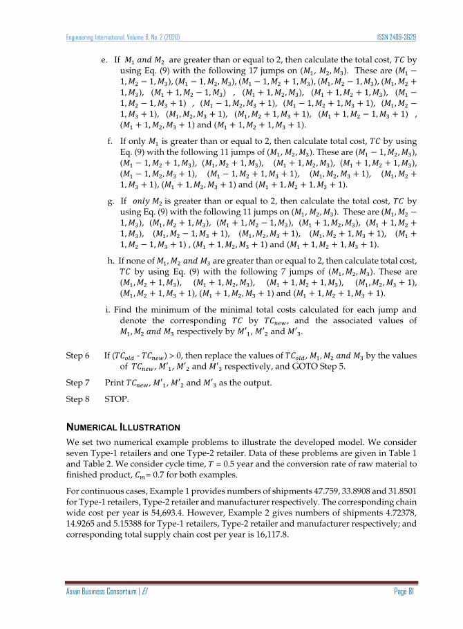
NUMERICAL ILLUSTRATION
We set two numerical example problems to illustrate the developed model. We consider seven Type-1 retailers and one Type-2 retailer. Data of these problems are given in Table 1 and Table 2. We consider cycle time, 𝑇 = 0.5 year and the conversion rate of raw material to finished product, 𝐶𝑚= 0.7 for both examples.
For continuous cases, Example 1 provides numbers of shipments 47.759, 33.8908 and 31.8501 for Type-1 retailers, Type-2 retailer and manufacturer respectively. The corresponding chain wide cost per year is 54,693.4. However, Example 2 gives numbers of shipments 4.72378, 14.9265 and 5.15388 for Type-1 retailers, Type-2 retailer and manufacturer respectively; and corresponding total supply chain cost per year is 16,117.8.

Islam et al.: A Green Integrated Inventory Model for a Three-Tier Supply Chain of an Agricultural Product (73-86)
Page 82 Engineering International, Volume 8, No. 2 (2020)
Table 1: Provided data for Example 1
Setup cost
Order cost
Holding Cost
(finished)
Holding cost
(raw)
Holding cost
(byprod.)
Cost of Each
shipment
Demand rate
Collection/ Production
rate
Type 1 Retailer 1 45 7 12 10,000
Type 1 Retailer 2 45 7 12 15,000
Type 1 Retailer 3 45 7 12 20,000
Type 1 Retailer 4 45 7 12 30,000
Type 1 Retailer 5 45 7 12 35,000
Type 1 Retailer 6 45 7 12 40,000
Type 1 Retailer 7 45 7 12 5000
Type 2 Retailer 30 5 8 18,000
Manufacturer 150 170 4 0.5 2 25 221,429 180,000
Supplier 550 0.7 221,429 290,000
Table 2: Provided data for Example 2
Setup cost
Order cost
Holding cost
(finished)
Holding Cost (raw)
Holding Cost
(byprod.)
Cost of Each
shipment
Demand rate
Collection/ Production
rate
Type 1 Retailer 1 105 4 20 1500
Type 1 Retailer 2 110 4.5 22 1500
Type 1 Retailer 3 115 5 23 1500
Type 1 Retailer 4 120 5.5 25 1500
Type 1 Retailer 5 125 6 25.5 1500
Type 1 Retailer 6 130 6.5 26 1500
Type 1 Retailer 7 90 7 27 1500
Type 2 Retailer 70 8 12 2500
Manufacturer 45 170 3.5 1.2 5 24 15,000 85,000
Supplier 550 2.2 15,000 150,000
Integral optimal solution to Example 1 in Table 3 shows that the minimal total cost 54,693.6 is obtained for 32 shipments of raw materials from supplier to manufacturer, 48 shipments of finished products from manufacturer to each retailer of Type-1 and 34 shipments of byproducts from manufacturer to Type-2 retailer. Integral optimal solutions to Example 2 are 𝑀1 = 5, 𝑀2= 5, 𝑀3= 15 and 𝑇𝐶 = 16,123.2, which are tabulated in Table 4.
Table 3: Integral optimal solution to Example 1
No. of shipments Shipment size Cost per year Supply chain cost per year
Type 1 Retailer 1 48 104.167 1606.58
Type 1 Retailer 2 48 156.25 1788.88
Type 1 Retailer 3 48 208.333 1971.17
Type 1 Retailer 4 48 312.5 2335.75
Type 1 Retailer 5 48 364.583 2518.04 54,693.6
Type 1 Retailer 6 48 416.583 2700.33
Type 1 Retailer 7 48 52.0833 1424.29
Type 2 Retailer 34 264.706 1265.76
Manufacturer 32 3459.82 37058.2
Supplier 2024.61

Engineering International, Volume 8, No. 2 (2020) ISSN 2409-3629
Asian Business Consortium | EI Page 83
Table 4: Integral optimal solution to Example 2
No. of shipments Shipment size Cost per year Supply chain cost per year
Type 1 Retailer 1 5 150 710
Type 1 Retailer 2 5 150 777.5
Type 1 Retailer 3 5 150 835
Type 1 Retailer 4 5 150 902.5
Type 1 Retailer 5 5 150 955 16,123.2
Type 1 Retailer 6 5 150 1007.5
Type 1 Retailer 7 5 150 975
Type 2 Retailer 15 83.3333 833.333
Manufacturer 5 1500 8832.34
Supplier 295
CONCLUSIONS
This study has presented a joint economic lot sizing coordinated inventory model for a three-tier supply chain involving a supplier, a manufacturer and multiple retailers. To make the environment green, the manufacturer uses byproducts on the demand of the consumers. Two types of retailers are considered in this model. Type-1 retailers’ retail manufacturer’s finished product, while Type-2 retailer trades manufacturer’s byproducts. We have found an analytical solution to the model. Though the model is developed based on agricultural product, it is also useful in the supply chain of non-agricultural product. Attached algorithm is suitable for finding integral solution. Analysis of optimal solutions to numerical example problems shows that the low shipment cost leads to frequent shipments of smaller sizes. This study might be extended in different directions. Equal lot sizing policy may not be fruitful in some situations. Hence, equal and/or unequal lot sizing policy may be adopted for better results. Also, one can extend this work by considering warehouse capacity constraint or service level constraint or back ordering policy.
REFERENCES
Abdelsalam, H.M., Elassal, M.M. (2014), Joint economic lot sizing problem for a three-layer supply chain with stochastic demand, Int. J. Prod. Econ. 155(1), 272–283.
Baboli, A., Fondrevelle, J., Tavakkoli-Moghaddam, R., Mehrabi, A. (2011), A replenishment policy based on joint optimization in a downstream pharmaceutical supply chain: centralized vs. decentralized replenishment, Int. J. Adv. Manuf. Technol. 57(1–4), 367–378.
Banerjee, A. (1986), A joint economic-lot-size model for purchaser and vendor, Decis. Sci. 17(3), 292–311.
Ben-Daya, M., and Al-Nassar, A. (2008), An integrated inventory production system in a three-layer supply chain, Production Planning & Control, 19(2), 97–104.
Ben-Daya, M., As’ad, R., Seliaman, M. (2013), An integrated production inventory model with raw material replenishment considerations in a three-layer supply chain, Int. J. Prod. Econ. 143(1), 53–61.
Ben-Daya, M., Darwish, M., Ertogral, K. (2008), The joint economic lot sizing problem: review and extensions, Eur. J. Oper. Res. 185(2), 726–742.
Ben-Daya, M., Hariga, M. (2004), Integrated single vendor single buyer model with stochastic demand and variable lead time, Int. J. Prod. Econ. 92(1), 75–80.
Islam et al.: A Green Integrated Inventory Model for a Three-Tier Supply Chain of an Agricultural Product (73-86)
Page 84 Engineering International, Volume 8, No. 2 (2020)
Ca ´rdenas-Barro ´n, L.E. (2007), Optimizing inventory decisions in a multi-stage multi-customer supply chain: a note, Transp. Res. Part E Logist. Transp. Rev. 43(5), 647–654.
Ca´rdenas-Barro´n, L.E., Teng, J.T., Trevin˜o-Garza, G., Wee, H.M., Lou, K.R. (2012), An improved algorithm and solution on an integrated production inventory model in a three-layer supply chain, Int. J. Prod. Econ. 136(2), 384–388.
Chen, T.H. and Chen, J.M. (2005), Optimizing supply chain collaboration based on joint replenishment and channel coordination, Transportation Research Part E: Logistics and Transportation Review, 41(4), 261-285.
Chung, S.L., Wee, H.M. and Yang, P.C. (2008), Optimal policy for a closed-loop supply chain inventory system with remanufacturing, Mathematical and Computer Modeling, 48(5), 867-881.
Gal, P.Y.L., Lyne, P.W.L., Meyer, E., Soler, L.G. (2008), Impact of sugarcane supply scheduling on mill sugar production: a South African case study, Agric. Syst. 96(1–3), 64–74.
Giri, B.C., Bardhan, S. (2015), A vendor-buyer JELS model with stock-dependent demand and consigned inventory under buyer’s space constraint, Oper. Res. Int. Journal 15(1), 79–93.
Glock, C.H. (2012), The joint economic lot size problem: a review, Int. J. Prod. Econ. 135(2), 671–686.
Goyal, S.K. (1977), Determination of optimum production quantity for a two-stage production system, Oper. Res. Q. 28, 865–870.
Goyal, S.K., Nebebe, F. (2000), Determination of economic production-shipment policy for a single-vendor single-buyer system, Eur. J. Oper. Res. 121(1), 175–178.
Gunasekaran, A., Lai, K., Edwin Cheng, T.C. (2008), Responsive supply chain: a competitive strategy in a networked economy, Omega Int. J. Manag. Sci. 36(4), 549–564.
Hariga, M., Glock, C.H., Kim, T. (2016), Integrated product and container inventory model for a singlevendor single-buyer supply chain with owned and rented returnable transport items, Int. J. Prod. Res. 54(7), 1964–1979.
Hellion, B., Mangione, F., Penz, B. (2015), Stability contracts between supplier and retailer: a new lot sizing model, Int. J. Prod. Res. 53(1), 1–12.
Hill, R.M. (1999), The optimal production and shipment policy for the-single vendor single-buyer integrated production-inventory problem, Int. J. Prod. Res. 37, 2463–2475.
Hoque, M.A. (2011), An optimal solution technique to the single-vendor multi-buyer integrated inventory supply chain by incorporating some realistic factors, Eur. J. Oper. Res. 215(1), 80–88.
http://digital-library.theiet.org/content/conferences/10.1049/cp.2014.1055
Islam, S.M.S. (2014), Single-vendor single-buyer optimal consignment policy for a seasonal product, HSTU Journal of Science and Technology 12, 59-66.
Islam, S.M.S., Hoque, M.A. (2014a), A vendor-buyer optimal consignment policy for a seasonal product with uniform distribution of demand, Malays. J. Sci. 33(2), 219–227.
Islam, S.M.S., Hoque, M.A. (2014b), An extension to single-manufacturer, multi-retailer consignment policy for retailers’ generalized demand distributions, Brunei International Conference on Engineering and Technology, Brunei, 1-3 November, pp.1-6.
Islam, S.M.S., Hoque, M.A. (2017), A joint economic lot size model for a supplier-manufacturer-retailers supply chain of an agricultural product, Int. J. OPS. 54(4), 868–885.
Islam, S.M.S., Hoque, M.A. (2018), Single-vendor single-buyer optimal consignment policy with generic demand distribution by considering some realistic factors, Int. J. Oper. Res. 31(2), 141-163.
Islam, S.M.S., Hoque, M.A. (2019), An optimal policy for three-tier supply chain for processing an agricultural product with a stochastic demand, Int. J. Services and Operations Management 33(3), 287-310.

Engineering International, Volume 8, No. 2 (2020) ISSN 2409-3629
Asian Business Consortium | EI Page 85
Islam, S.M.S., Hoque, M.A., Hamzah, N. (2017), Single-supplier single-manufacturer multi-retailer consignment policy for retailers’ generalized demand distributions, Int. J. Prod. Econ. 184(1), 157–167.
Islam, S.M.S., Yasmin, M.J. and Hossain, R. (2020), A joint economic lot size inventory model for a supply chain problem of multiple agricultural products having same properties, Int. J. of Latest Trends in Engineering and Technology 18(2), 37-42.
Jaber, M.Y. and Goyal, S.K. (2008), Coordinating a three-level supply chain with multiple suppliers, a vendor and multiple buyers, Int. J. Prod. Econ. 116(1), 95-103.
Khouja, M. (2003), Optimizing inventory decisions in a multi stage multi-customer supply chain, Transportation Research Part E: Logistics and Transportation Review, 39(3), 193-208.
Kim, T., Glock, C.H., Kwon, Y. (2014), A closed-loop supply chain for deteriorating products under stochastic container return times, Omega 43(1), 30–40.
Lee, W. (2005), A joint economic lot size model for raw material ordering, manufacturing setup, and finished goods delivering, Omega Int. J. Manag. Sci. 33(2), 163–174.
Moncayo-Martı ´nez, L.A., Zhang, D.Z. (2013), Optimising safety stock placement and lead time in an assembly supply chain using bi-objective MAX–MIN ant system, Int. J. Prod. Econ. 145(1), 18–28.
Munson, C.L. and Rosenblatt, M.J. (2001), Coordinating a three-level supply chain with quantity discounts, IIE Transactions, 33(5), 371-384.
Sari, D.P., Rusdiansyah, A., Huang, L. (2012), Models of joint economic lot-sizing problem with time-based temporary price discounts, Int. J. Prod. Econ. 139(1), 145–154.
Sarmah, S.P., Acharya, D., Goyal, S.K. (2006), Buyer vendor coordination models in supply chain management, Eur. J. Oper. Res. 175(1), 1–15.
Wang, C., Huang, R., Wei, Q. (2015), Integrated pricing and lot-sizing decision in a two-echelon supply chain with a finite production rate, Int. J. Prod. Econ. 161(1), 44–53.
--0--
Islam et al.: A Green Integrated Inventory Model for a Three-Tier Supply Chain of an Agricultural Product (73-86)
Page 86 Engineering International, Volume 8, No. 2 (2020)
How to Cite:
Islam, S. M. S., Hossain, R., & Yasmin, M. J. (2020). A Green Integrated Inventory Model
for a Three-Tier Supply Chain of an Agricultural Product. Engineering International, 8(2), 73-86. https://doi.org/10.18034/ei.v8i2.505