A Graphical Method

8/9/2019 A Graphical Method

http://slidepdf.com/reader/full/a-graphical-method 1/8

Nor d ic Hy dr o log y 27 4), 1996,247-254

No pan may

be

reproduced by any proce\ ; without complete reference

Graphical Method

for Storage Coefficient Determination from

Quasi Steady State Flow Data

ZeUi Sen

Technical U niversi ty of Istanbul , Turk ey

A simp le, approximate but practical graphical method is proposed for estimating

the storage coefficient independently from the transmissivity value, provided

that quasi-steady state flow data are available from a pumping test. In the past,

quasi-steady state flow distance-drawdown data have becn uscd for the detcrmi-

nation of transmissivity only. The method is applicable to confined and leaky

aquifers. The application of the method has been performed for various aquifer

test data available in the groundwater literature. The results are within the prac-

tical limits of approximation com pared with the unstcady state flow solutions.

Introduction

T h i e m 1906) obta ined a quasi -s teady s ta te groundwater movement equat ion for

smal l d iameter wel l s in confined aqui fers as

where Q i s the constant pump discharge; T is aquifer t ransmissivity;

s

and s2 are

draw dow n m easur em ents in observation wel l s which a re a t rad ia l d is tances

rl

and r2

respect ively, fr om the main well center, see Fig. 1). Fo r the val idity of Eq. l ) , the

aqui fer must be confined wi th inf in ite area l ex tent, mu st be hom ogeneous, i sot ropic

and of uni form th ickness , and the well mu st have com ple te penet rat ion .



ekai

en

Fig.

1

Confined aquifer configuration with main and observation wells.

On the other hand, in the case of leaky aquifer steady state flow, the valid expres-

sion was given first by D e Glee (1930 ) as

in which s, is the steady state drawdown in the piezometer at distance r from the

main well. Ko(rlL) represents the modified Bessel function of the second kind and

zero order, and finally, L is the leakage factor. It is clear from Eqs. (1) and (2) that

the draw down changes with distance, and furthermore, drawdow n versus the loga-

rithm of the distance plots along a straight line for Eq. (2) only when rlL is sma ll (see

remarks to H antush -Jaco b s method in Krusem an and de Ridder 1990; pages 77-80).

In practice, Eqs. (1) and

(2)

are used for determining the transmissivity only.

Krusem an and de Rid de r(l9 90) have presented procedures that can be applied in de-

termining the transmissivity of confined or leaky aquifers. Such procedures do not

require comp lete pump test data, but depend on steady state measurements after long

times. The best way to ensure a reliable estim ate of the storage coefficient of a con-

fined or leaky aq uifer is to ana lyze time series of draw dow n during a pumping test.

Time series of draw dow n from just on e observation well reveals possible positive or

negative boundaries within the aquifer and problems with matching type curves in-

dicate heterogeneity, (yen and Al-Baradi 1991); if time series are available from a

number of observation wells distributed around the pumping well then the analysis

of aquifer characteristics is further improved. Steady state data cannot be expected

to reveal this, especially if da ta are only available for a few wells.

However, if no time series are available one can use a quasi-steady state draw-

down data to roughly estimate the storage coefficient. In the following a simple

graphical procedure for estimating the aquifer storage coefficient in addition to the

transmissivity determination f rom a quasi-steady state distance-drawdow n record.



Gra phica l Method for Storage C oe fic ie nt Determination

Storage Coefficient

The storage coefficient plays a vital role for the transient behavior of groundwater

flow and in the estimatio n of the withdrawal volume of groundw ater from an aqui-

fer. Consequently, its precise determination is one of the prerequisites in groundw a-

ter resources assessments and managem ent in any region. Unfortunately, some ana-

lytical procedures for aquifer test data evaluation by either type curve matching or

straight line methods, yield reliable transmissivity values but questionable storage

coefficient estim ates. For instanc e, the Co oper and Jacob (1946) recovery straight

line method p rovides e stim ates of transm issivity only. Furtherm ore, the reliability of

storage coefficient estimations obtained from the Papadopulos and C ooper (1 967)

and

the Sen (1991 ) methods are highly questionable. The idea of estimating the stor-

age coefficient from the volume of the cone of depression is due to Wenzel (1937),

who used drawd own d ata from a large number of observation wells to calculate the

volume of the cone of depression and estimate the specific yield of an unconfined

aquifer near Grand Island, Nebraska. Bennett et a1 (1967) applied the method to aq-

uifer tests from the Punjab Region in Pakistan. Attempts to estimate the storage co-

efficient,

S

from quasi-steady state flow measurements without type curve expres-

sions are due to en (1987 ) who defined as a ratio of two volumes

where

Qt

is the volume of abstracted water during time period

t

with constant dis-

charge Q and V D s the depression cone volume. He then obtained theoretically, a

rather sophisticated expression for V

leading to a complicated expression for

S.

However, on what follows a straight-forward graphical procedure is suggested

which gives firstly an estimate of the depression cone volume from the quasi-steady

state flow data and secondly, an estimate of the storage coefficient according to Eq.

(3).

Quasi Steady State Flow

Theoretically, Eqs. ( I ) and

(2)

represent a straight line on a semi-logarithmic paper

with drawdown versus distance of each observation well from the main well center.

Consequently, two or preferably m ore observation w ells will be used in the practical

application for the construction of such an experimental straight line. It is well

known that the slope of the line is related to the transmissivity. It is suggested here-

in that the revolution volum e of the same straight line about the draw dow n axis is re-

lated to the depression cone volume,

V

If this volume is known, then the storage

coefficient can be estimated from E q. (3). The necessary steps for the suggested pro-

cedure are as follows:



ekai

en

Fig. 2.

Schematic distance-drawdown plot.

a) Plot the observed late draw dow n data from obse rvation wells located at various

distance s on a semi-log paper with dra wd ow ns on the vertical linear axis and the

corresponding distances on the horizontal logarithmic axis as in Fig. 2. This is

one of the major steps in the Jacob s traight line me thod.

b) Draw the best-fit straight line through the scatter points of data.

c) Extend this line in both directions until the points of interse ction with the vertical

and horizontal axes are obtained.

d) Determine the slope,

As

and then the intersection va lues, sLa nd rU o f this line on

the draw down and the distance axes, respectively. Clearly, ruc orr esp on ds phy si-

cally to the radius of influence and the drawdown value beyond this distance is

approximately zero everywhere within the aquifer. Besides, the drawdown inter-

section has the distanc e, r~ from the main well cente r see Fig. 2).

e) It is well known that the slope of the fitted line can be found theoretically from

Eqs. I ) and

2)

as

which has been used so far in the literature for the transm issivity estima tion.

f)

Calculate the area,

A

of the triangle constituted by the two axes and the fitted

straight line in Fig.

2.

Hence,

which is logically related to the depression cone vo lum e

g) Consider the revolution of the area below the fitted line abou t the draw dow n axis

but with back transformation of distan ces to linear scale which yield s the depre s-

sion cone volume estimate as



Graphical Method for Storage oefJicient Determination

h) The substitution of this volume expression into Eq.(3) gives the storage coeffi-

cient estima te as

Field pplications

Th e validity of the methodology deve loped here fo r the identificatio n of storage co-

efficient from quasi-steady state flow in confined aquifers and for perfectly steady

state flow in leaky aquifers is presented through applications to field data already

presented by Krus ema n and de Ridd er (1 990; Tables 3.1 an d 4.1). First of all results

of the application of Theim s method to data from pum ping test >> OudeKorendijk<c

are reproduced herein in Table 1 from Table 3.2 given by the same authors. The

pumping discharge is = 788 mYday and the quasi-steady state flow is reached af-

ter 83 0 min.

Table Aquifer Test Data and Results

Averages

385 5.94

The plots of distance-drawdown data on a semi-logarithmic paper as shown in

Fig. give two points which are conn ected by straight lines, and the proce dure in the

previous section gives the relevant quantities a s show n in the secon d part of the ta-

ble. Although the storage coefficient estimates of the proposed method are some-

what larger than the estimates from Theis and Jaco b meth ods, in their order of mag -

nitude they show very good agreement with Theis (1.6 ~1 0- 4) , nd Jacob (1 .7 ~1 0- 4,

4.1 x10-4 and 1 .7 ~ 1 0 -4 ) ethod estimates, (Kruseman and de R idder 1990).

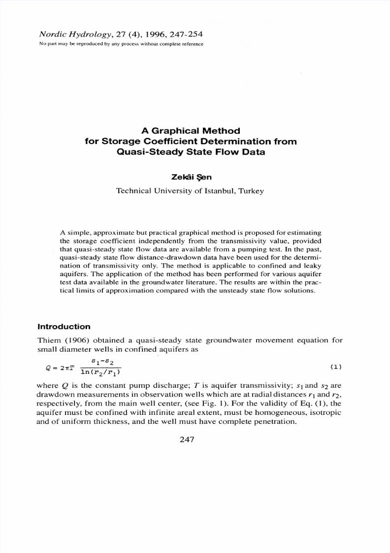
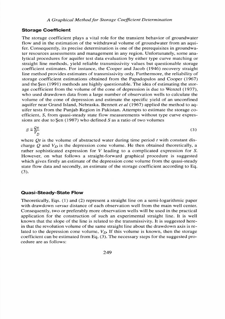
The method is also applied to the transient Qud e Korend ijkk da ta given by Kruse -

man and de Ridder(l990; Table 3.1). The plots of distance-drawdown values from

two piezometers at distances 3 0 m and 9 0 m after 140 min, 30 0 min, 60 0 min, and

830 min from the aquifer test start are shown in Fig. 4, with four parallel straight

lines. Th e implementation of the steps in the previous section gives rise to relevant

data as show n in Table 2 for the various cases.



Zekai kn

Fig. 3. Distance-drawdown plot for Qude Koredij data.

Table 2 Storage Coefficient Determination.

Time s r r S L S Y L S

(min) (m) (m) (n1) (m)

X

10-4) (m) (x10-4)

140 0.76

450

.0 2.04 3.62

10.0 3.76

300 0.76 590

.0 2.12 4.53

10.0 2.97

600 0.76

710 .0 2.19

6.23 10.0 4.13

830 0.76 785 .0 2.20

7.12 10.0

4.78

Averages 5.35 10.0 3.91

Fig. 4. Distance-drawdown plot for Jacob method with Qude Korendijk data.



G rap hic al Method for Stora ge CoefJicient Determination

It is interesting to notice in this table that chang es in the time duration lead to stor-

age coefficient values with the same order of magnitude. M oreover, they a lso com-

pare very well with the results obtained from other techniques. It seems from the

sixth column that the estimated storage coefficient changes with time and such

changes are due to the heterogeneities of the aquifer portion within the depression

cone and explained in detail by $en (1994). However, according to Kruseman and de

Ridder (1 990, page 7 0) no heterogeneities can be detected from analysis of transient

data. According to them the apparent increase of S with time may be due to leakage.

A critical point in the application of the method appears in choosing the lower dis-

tance value. Logically, it might be taken as equal to the well diameter. How ever, the

choice of any small distance has no significant practical effect on the final storativ-

ity es timation. To il lustrate th is , r ~ ,s chosen as equal to 1 O, and the corresponding

drawdown as well as the storativity calculations are presented in the last two col-

umns. It is obv ious that in sp ite of the significan t difference in the rLvalues, the stor-

ativities do not deviate significantly from one another, i.e. not by order of magni-

tude. The model assum ptions that can explain the relative significance and systemat-

ic deviations between the coefficients estimated by various methods including Theis

and Jacob procedure s are already presented by $en (1988).

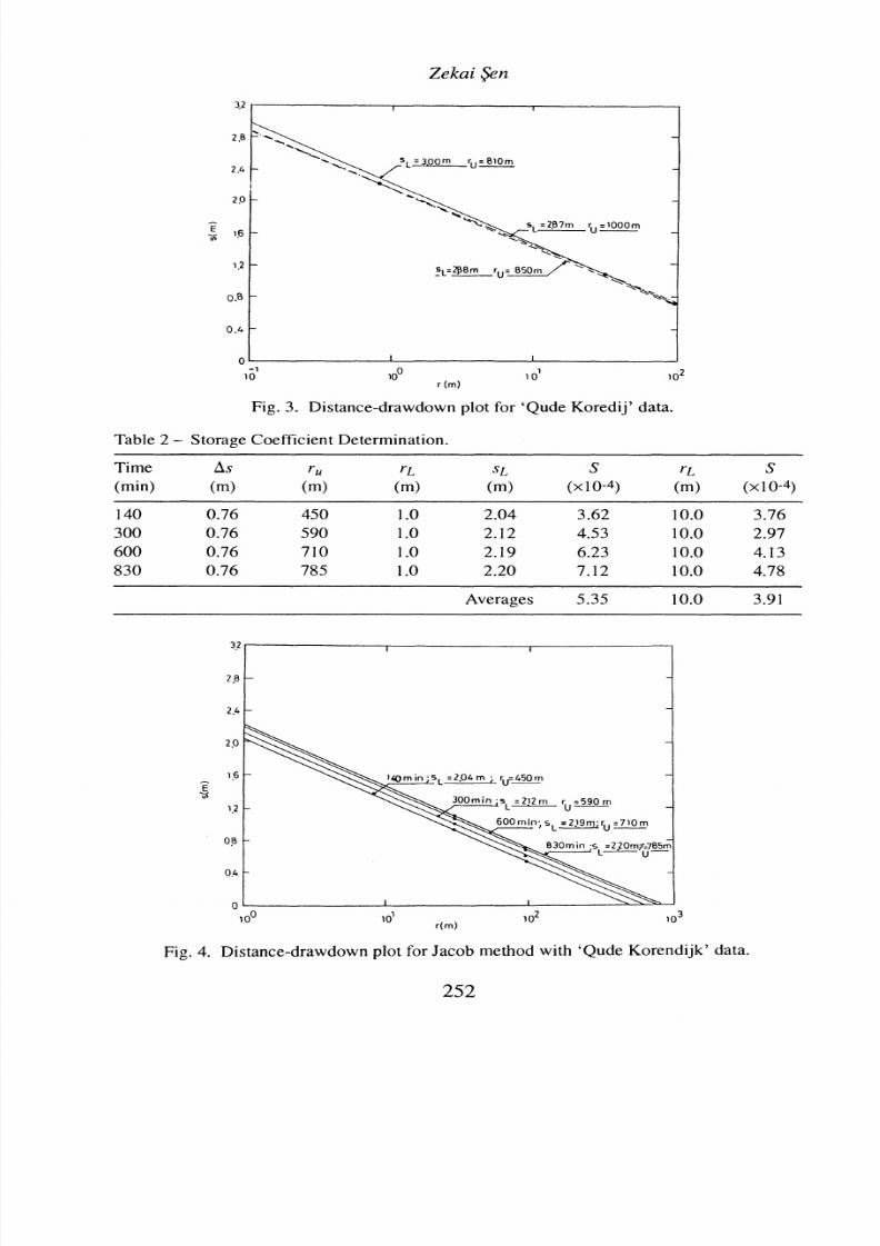
Finally, the leaky aquifer steady state flow data Dalem are also adopted from

Kruseman and de Ridder (1990; Table 4.1). The distance-drawdown plot is repro-

duced in Fig. 5. The pump discharge is 761 m31day and the steady state is reached

after about 0.4 days from the pump start. The substitution of the slope value from

Fig. 5 into Eq. (4) yields that T 2,02 0 m2lday. Add itionally, the necessary quan titi-

es for the storage coefficient calculation are r 1,100 m; SL 0.32 m; and r~

=

6 m.

The substitution of these values into Eq . (6) yields that S 1.4x10-?. Th is value

compares very well with the storage coefficient estimates obtained from the applica-

tion of other techniques such as the Hantush inflection point and the Hantush type

curve methods which gave 1 . 7 ~0-3 , and 1 .5 ~1 0- 3 ,espectively, (Kruseman and de

Ridder 1990).

F i e l d d a t a

n

I

t

I I

Fig.

d

r 6

10' l o 2

Leaky aquifer distance-drawdown

r

m )

plot for

Dalem

data.

53



ekai en

onclusions

An approx imate m ethod ha s been deve loped fo r ideq ti fy ing the s to rage f rom quas i -

s t eady s t a te f low in conf ined and s t eady s t a te f low da ta in l eaky aqu ife rs . Th e bas i s

concep t i s r e la ted to ob ta in ing the depres s ion co ne vo lume es t imat ion f rom a d i st an-

ce-draw dow n plo t on a sem i- logar i thmic paper . Def in i t ion of s tora tiv i ty as the rat io

o f abs t r ac ted wa te r vo lu me to the depres s ion con e vo lume leads to a s imple fo rmula

for ca lcula t ing i t s value . The s torage coeff ic ient procedure resul ts f rom the metho-

dology p resented in th is pape r conform pract ica l ly very wel l wi th the results obta i -

ned f ro m t radi tional me thod s on the bas is of order of mag ni tude. Th e use of the pro-

posed m ethod i s r ecom me nded if n o t ime s e r ies a re avai lab le showing the comple te

chang e o f

d raw dow n w i th t ime dur ing a co mp le te aqu i f e r t es t.

References

Bennett, G. D., Rehma n, Sheikh , I. A., and Sabir, A. 1967 ) Analysis of aquifer tests in the

Punjab region of west Pakistan, U.S. Geological Survey, Water Supply Paper 1608-G.

Cooper,

H.

H., and Jacob, C. E. 1946) A generalized graphical method for evaluating forma-

tion constants and summarizing well field history,

Am.

Geop hys. U nion Trans., Vol. 27, pp.

526-534.

De Glee, G. J. 1930 ) Ove r groundwaterstromingen bij teronttrekking door middel van putten,

Thesis, J. Waltman, Delft The Netherlands), 175 pp.

Kruseman, G . P., and de Ridder, N. A. 1990 ) Analysis and evaluation of pumping test data,

Bulletin 11, Institute for Land Reclamation and Improvem ent, Wageningen, pp. 41-69.

Papadopulos, I. S. , and H. H., Cooper 1967 ) Drawdow n in a well of large diameter,

Water

Resour. Res. , Vol. 3

pp. 241-244.

Sen, Z. 1987 ) Storage coefficient determination from quasi-steady state flow, Nordic Hydro-

logy , Vol.

18, pp. 101-110.

Sen, Z. 1988) Dimensionless time drawdown plots of late aquifer test data, Ground Water,

Vol. 26, No. 5 , pp. 615-624.

Sen, Z. 1991) Recovery type curves for large diameter wells, Nordic Hydrology, Vol. 22, pp.

253-261.

Sen,

Z.

1994) Hydrogeophysical concepts in aquifer test analysis,

Nordic Hydrology, Vol. 2.5,

pp. 183-192.

Sen, Z., and Al-Baradi, A. 1991 ) Sample functions as indicators of aquifer heterogeneities,

Nordic Hydrology, Vol.

2 2 ,

pp. 37-45.

Thiem. G. 1906)

Hydrologische Methoden,

Gebhardt, Leipzig, 5 6 pp.

Wenzel, L. K. 1937) The Thiem method for determining the permeability of water-bearing

materials and its,application for determination of specific yield. U.S. Geological Survey,

Water Supply Paper 679.

Received: December, 1994

Address

Istanbul Technical University,

Revised version received: 12 October, 1995

Meteorology D epartment,

Accepted: 30 November, 1995

Maslak 80 626, Istanbul, Turkey.

A Graphical Method

Documents

Transcript of A Graphical Method