1

A Graph-based Automatic Services Composition based on Cost Estimation Heuristic

Yunsu Lee1, Boonserm Kulvatunyou1, Minchul Lee1, Yun Peng2, Nenad Ivezic1

1Systems Integration Division, National Institute of Standards and Technology

2Computer Science and Electrical Engineering, University of Maryland, Baltimore County

ABSTRACT

Currently, both software and hardware are being virtualized and offered as services on the internet.

Companies have an opportunity to improve their workflows by composing services that best suit

their quality and cost requirements. However, as more services become available, computer-aided

services discovery and composition become essential. Traditional service representation and

planning algorithms do not adequately address non-functional characteristics, large numbers of

similar operators (i.e., services), and limited numbers of objects (i.e., inputs and outputs per

service). This paper analyzes existing work in automatic services composition, service

representation and planning algorithms and proposes a new framework to address those needs. It

proves that the proposed framework provides an admissible heuristic based on cost estimations

that guarantee a minimum cost solution, if one exists.

1. Introduction

Software and hardware components are trending toward modular atomic services (rather than large

monolithic applications) on the cloud. This trend enables companies to improve their operations

by choosing best-of-breed services for specific functions. For example, a food manufacturer can

compose their production planning using its in-house information gathering services and external

best-of-breed recipe reformulation services based on ingredient characteristics of a given batch.

Companies can also quickly respond to disruptions and the customer’s changing needs by

composing services to meet new requirements. Cloud platforms or marketplaces such as the Smart

Manufacturing Platform proposed by the Smart Manufacturing Leadership Coalition (SMLC) [1-

2] facilitate this trend. The open access of such marketplaces means that customers may encounter

a large number of available services.

In such situation, computer-aided services composition is essential. For example, a user can write

a rule to detect an event from a Customer Relationship Management (CRM) service which then

triggers an email service to send the event details to a particular address. Despite such simple

services composition structure, services that composed together need to be functionally and non-

functionally compatible. For that, today’s existing tools provide only a simple categorization of

available services. Therefore, it is a challenge for the user to manually determine the functional

and non-functional compatibility between services. In an enterprise business environment, the

composition task is typically more complex than the simple email trigger example above.

Therefore, a computational aid is essential for making services search and composition more

efficient and effective in such an open marketplace for service offerings.

2

There are two primary issues in developing a computational aid for services search and

composition. First, currently available computer interpretable service descriptions are insufficient.

Typically, services have functional and non-functional characteristics. Currently, there are several

existing standards and efforts to describe the characteristics of services. WSDL (Web Services

Description Language) [3] and Open API [4] are the standards used by many software vendors.

However, these standards focus more on the non-functional characteristics such as the transfer

protocol specification that are essential for ensuring the secure and reliable transmission of

information between different services. The standards offer no more than inputs and outputs of the

service and their formats in term of the functional characteristics. Those input and output formats

provide insufficient information for the automated composability analysis that supports finding

and evaluating of combined components to perform a desired task. The other issue is that there is

no automatic computational method that is best suitable for the services composition problem.

In existing automatic services composition works such as in [5-7], services were represented as

operators and user’s requirements were represented as the initial and the goal conditions. Then,

the services composition problem was formulated as a classical planning problem to find a set of

services (operators) that can transition the initial condition to the goal condition while satisfying

input/output and pre/post-conditions of the services. However, Artificial Intelligent (AI) planning

methods for solving classical planning problem have a few drawbacks when applying them to the

services composition problem.

First, these methods are typically applicable to a problem with a small number of possible operators

(e.g., moving blocks) and a large number of objects (e.g., hundreds of blocks). On the other hand,

services composition problem typically deals with a large number of operators (huge number of

services on the cloud), and a limited number of objects (e.g., getting a flight, renting a car, and

registering a hotel, transforming a piece of information or a workpiece). Second, AI planning

methods do not deal with the situation where there are a large number of same or similar services

(e.g., hundreds of travel agent services, tens of possible scheduling algorithms, or manufacturing

processes). Lastly, AI planning methods are typically computationally expensive due to the

embedded Sussman anomaly avoidance [8-9]. For services composition problems, however,

interleaving conditions between sub-goals in Sussman anomaly can be detected and prevented a

priori.

The main objective of this research is to develop a computer-aided services search and composition

framework for an open cloud service marketplace environment. To realize such a framework, this

paper presents a method for representing a service and a novel graph-based algorithm using a cost

estimation heuristic for services search and composition. A proof is provided that the heuristic

guarantees the minimal cost solution subgraph if one exists. Finally, the results of an experimental

comparison with other algorithms are presented. They indicate the exceptional performance and

scalability of the algorithm.

2. Related Work

In this section, works closely relevant to our research are presented. First, we review existing

specifications for service descriptions. Second, we dive into the detail of functional representation

within the service description. Third, a state-of-the-art review on existing automatic services

composition methods is provided. Two major means to automatic service search and composition

methods are investigated, AI planning-based and graph search-based.

3

2.1 Service description method

The rise of Internet computing resulted in Web-based interface definition languages. W3C (World

Wide Web Consortium) WSDL [3] is a predominant one. Basic semantics and structure of WSDL

are similar to that of programming language APIs (Application Programming Interfaces). More

recently, a service description specification called Open API [4] has been introduced. A WSDL

and Open API function, however, does not necessarily tie to a source code function – allowing it

to represent the aggregate, business- or user-oriented functionality. WSDL also allows for rich

description via XML (eXtensible Markup Language) Schema specification of the input and output

and via structured annotation on any information element. However, WSDL does not standardize

any semantics of the annotation. The strength of WSDL is in the standardized semantics of its

transfer protocol specification that is essential for measuring non-functional compatibility.

Several efforts have been proposed to enhance how Web services descriptions describe function.

Prior work in this area include OWL-S (Web Ontology Language for Ser-vices) [10], SAWSDL

(Semantic Annotations for WSDL and XML Schema) [11], and WSMO (Web Service Modeling

Ontology) [12]. SAWSDL enhances WSDL and associated XML Schema semantics by adding

attributes to WSDL entities that point to concepts in a semantically rich ontology. SAWSDL does

not define any additional semantics to describe functionalities; it only provides a mechanism to

link to the referenced semantics.

OWL-S (Semantic Markup for Web Services) and WSMO (Web Services Modeling Ontology)

are similar in their efforts to define ontologies for service descriptions (called Service Profile in

OWL-S and Capability in WSMO). Both of them rely on a similar set of elements that describe 1)

pre- and post-conditions associated with information used and produced by a service and 2) pre-

and post-conditions associated with the states of world before and after an execution of the service.

WSMO defines a Goal concept in addition to the Capability concept. SAWSDL also informally

describes the Goal notion as a Web service request. In WSMO, a Goal is described by a post-

condition. The functional description in the Goal expresses requirements and is used for searching

and matching a Capability. If the post-condition in the Goal matches the one in the Capability,

then the service is relevant. Such notion of Goal and Capability matching is part of the

composability analysis.

Both OWL-S and WSMO also allow for a detailed functional description of a service by specifying

a process specification. Such provision needs to be evaluated for complexity at the time of

composability analysis. Semantic links between the service and ontological concepts of functions

as in SAWSDL can be more computational friendly.

While OWL-S and WSMO define more expressive models for service descriptions, they lack

provision for describing functions or domain-specific characteristics of the capability. For example,

one order processing service may be able to process several order types including the new-item

outbound order, inbound (return) order, and replacement order while another order processing

service may only be able to process a new-item outbound order. Such differences in service scope

must be known in order to effectively compose the services, yet current practices do not permit

expression of the constraints on scope. In addition, a common semantic model for world states is

needed when composing services from heterogeneous resources. Such problems have motivated

several efforts to develop domain specific reference ontologies. Domain specific ontologies have

been developed in the biological, biomedical, and financial domains. Ontologies for the industrial

manufacturing domain are currently more fragmented [14-18], but recently, an Industrial

4

Ontologies Foundry (IOF) [13] has been formed to develop coherent ontologies across

manufacturing.

2.2 Representing function

Enhancing service description with better description of function is necessary for more precise

composability analysis. This section of the paper reviews works in function representation theories

and function modeling. Studies about function modeling and representation have been prevalent

in the product design discipline to represent the “functional requirement”.

First, we investigate the notion of function within the term “functional requirement.” According

to Glinz [19], there are two widely accepted definitions of the term, functional requirements, within

the requirement engineering research area. The first definition emphasizes function. Suzanne and

James [20] stated that a functional requirement specifies “requirement that specifies a function that

a system or system component must be able to perform”, while Sommerville [21] stated that

functional requirement specifies “what the system should do”. Despite using different terms, they

commonly stated that functional requirement specifies function. The second definition emphasizes

behavior. Anton [22] stated “functional requirements describe the behavioral aspects of a system”.

And Davis [23] stated “those requirements that specify the inputs (stimuli) to the system, the

outputs (responses) from the system, and behavioral relationships between them; also called

functional or operational requirements.” According to IEEE 830 [24], functional requirements

should define the fundamental actions required to process the inputs and generate the outputs. This

literature provides the evidence that the notion of “function” is closely related with the term

“behavior” and “action.”

A number of existing works classify functions into two categories. Chittaro and Kumar [25]

classified functions as the “operation function” or the “purposive function”. Chkrabarti [26]

classified them as the “intended behavior” or the “purpose”. Charkrabarti later on with Bligh [27]

classified them as the “action” or “effect”. On the other hand, Deng [28] called them “action

function” and “purpose function”. However, the paper also raises an issue that the distinction

between them is not clear-cut. This is because an action function may also contain design/purpose

function, as it relates to intended and useful behavior. On the other hand, a purpose function may

also require a certain action, even though this is not explicitly mentioned.

Chandrasekaran and Josephson [29] proposed a widely-accepted formal definition of function that

cover all of the above notions. He classified functions as “device-centric” or “environment-centric”.

A device-centric function is formally represented with predicates over the variables associated

with the internal structural elements of a system. (The term, system, here can be any of device,

service, component and so on.) It corresponds to the behavior of a given system and covers the

operational function in Chittaro and Kumar [25], the intended behavior in Chakrabarti [26], the

action in Chakrabarti and Bligh [27], and the action function in Deng [28].

The environment-centric function, on the other hand, is represented with predicates (state) over

elements (resource) external to the system and with a relationship to the device-centric function.

Such relationship is called “Mode of Deployment”. It allows for the assignment of a specific

context to the device-centric function. For example, the environment-centric function of the

electric lamp is “room illumination” when the lamp is placed (i.e., deployed) in a room with the

switch turned on. Thus, the device-centric function of the electric lamp can be individuated as

“illuminate something or somewhere”. Chandrasekaran [30] explains that the device-centric

5

function is the mean to achieving the environment-centric function and this statement also implies

that the environment-centric function has a close relation with the “purpose”. Thus, the

environment-centric function covers the purposive function in Chittaro and Kumar [25], the

purpose in Chakrabarti [26], the effect in Chakrabarti and Bligh [27], and the purpose function in

Deng [28].

In section 3, we use Chandrasekaran and Josephson work to formally represent service and the

characteristic of function the service possesses. Such representation is needed that goes beyond

the mere input, output, and function label in today’s popular service description standards.

2.3 Approaches for automatic services composition

In the past decade, a number of works in automatic services composition (specifically web services

composition) appeared in literature. Artificial Intelligence (AI) techniques, specifically AI

Planning techniques, were used for automatic services composition such as in [5-7, 35]. However,

graph search methods were also popular such as in [36-38]. In the following sub-sections, an

overview and characteristics of these two approaches are discussed.

2.3.1 AI planning approaches

Two kinds of AI planning-based approaches are distinguished. The first one is the domain-

independent AI Planning approaches that try to solve general planning problem without reliance

on domain-specific knowledge. The other is the domain-specific AI Planning approaches that use

domain heuristics to help to solve the problem.

2.3.1.1 Domain-independent planning

In practice, it is not feasible to develop domain-independent planners that work in every possible

domain. Thus, typically, most of the domain-independent planning approaches make simplifying

assumptions to restrict the set of domains such as finite system, and deterministic outcome.

A class of the domain-independent planning approaches is the GraphPlan1 which is a general-

purpose planner for STRIPS2-style problems [31]. The operation of GraphPlan consists of two

phases. In the first phase, a forward search is used to build a planning graph. In this phase,

GraphPlan extends the planning graph forward from the initial state until a necessary (but

insufficient) condition for plan exit is met. In the second phase, a regression search is performed

to extract a sufficient plan. In this phase, backward search is performed from the goal, looking for

a correct plan.

Another class of the domain-independent planning approach is Compilation-based Planning.

These planners try to solve the planning problem by converting it into another classical planning

problem such as SAT (Planning as Satisfiability) [32], CSP (Planning as Constraint Satisfaction

Problem) [33], or ILP (Planning as Integer Linear Programming) [34]. Typical procedure of the

compilation-based planning approaches is as follows: 1) set the maximum plan length to k, 2)

encode the plan as a generic planning problems, 3) solve the problem using an off-the-shelf solver

1 Despite its name GraphPlan is not considered a graph-based planning approach because the problem is not translated

into a graph. Rather it dynamically generates possible solution graphs and prunes for a valid one similar to the Planning

as Satisfiability.

2 STRIPS stands for Stanford Research Institute Problem Solver.

6

and 4) if a solution is found, decoded the generic planning problem into domain terms; otherwise,

repeat the procedure after increasing the value of k until a plan is found.

2.3.1.2 Domain-Specific Planning

Domain-specific planning (DSP) is also known as configurable planning. DSP exploits one or a

few planning recipes that are specific to a particular type or domain of problems. For example, a

recipe for traveling to a distant destination may be 1) buying a ticket for a flight from the local

airport to the remote airport, 2) taking a public transportation to the local airport, 3) flying to the

remote airport, and 4) taking a public transportation to the final destination. Such recipes narrow

down the search space rather than consider every combination of transportation modes, sequences,

providers, and routes as required in the domain-independent method.

Hierarchical Task Network (HTN) Planning methods enable domain-specific planning. HTN

planners divide the problem into tasks (activities), rather than goals and methods, and decompose

tasks into subtasks. HTN Planners provide a construct to encode a recipe as a collection of methods

and operators. Each recipe provides a way to solving a certain problem. As a result, the planning

system does not necessarily have to repeatedly derive solutions. However, disadvantages of the

HTN Planning is that writing a domain-specific knowledge can be more complicated than just

writing classical operators.

Intuitively, AI planning approaches can be the solution for automatic services composition, which

explains why a number of services composition researches are relying on them [35]. However, the

computational complexity of the AI planning approaches is typically very high. Moreover, they

do not guarantee that a solution will be found when one exists.

2.3.2 Graph-based planning approaches

In Graph-based planning approaches, composition problems are represented as a graph. Services,

initial states, and goal states can be modeled as vertices, while input and output can be modeled as

edges between vertices. This can also be done vice versa. Graph search algorithms find paths – a

set of valid edges connecting the initial state to the goal state [36-38]. It is straightforward to

construct an adjacent list or a matrix to represent a service network graph and obtain the shortest

path from the source to the goal vertex using existing well-known shortest path finding algorithms

such as the Bellman–Ford Algorithm and Dijkstra Algorithm. [39-42].

However, there are some limitations in the existing graph-based planning approaches. First, the

existing approaches only support a graph with single input and single output per vertex. In addition,

the existing methods only work with a single cost model and hard constraint associated with each

of the edges. In this paper, realistic services composition problems with multiple cost models, hard

constraints, as well as soft constraints (e.g., preferred vendors) are considered. To that effect, the

existing methods for finding the shortest path cannot deal with these additional parameters.

2.3.3 Automatic services composition

While services composition can be viewed as a classical planning problem where AI planning

approaches can be applied, graph-based planning approaches are more suitable from the

perspective of computational efficiency. The main short-coming with AI planning is that they need

to check for interleaving between sub-plans at every planning step. However, interleaving is less

of an issue in the services composition problem because operators are more specific as the next

service can be applied only if its pre-condition and input are compatible with the post-condition

7

and output of the previous service. In other words, interleaving can be virtually prevented by

constructing a composition-network graph from services compatibility and by applying cycle

detection and elimination. As such, this paper extends and addresses the aforementioned

shortcomings in graph-based planning. To that end, the next section first describes the formalism

for service description necessary to represent the additional parameters by applying the function

representation theories reviewed in Section 2.2. The representation is then used in the graph-based

planning algorithm proposed in Section 4.

3. Function and Service Representation Method

In this section, we (1) consider what is needed to make services composable, (2) whether the

condition differs in different types of services (software or hardware) and (3) whether the

requirements for composition are functional or non-functional.

3.1 Functional characteristics

Functional characteristics of a service are related to the notion of function. For a clear definition

of function, we investigated existing works in the function representation research area and found

that there are a number of definitions in existing works as described in the related work section.

These researches show that ‘behavior’ and ‘effect’ are two important aspects of the function notion.

The term ‘behavior’ means change objectively observable without any context. As we look at

motorized toggle clamp as an example, it has a behavior that generates a clamping force when it

is fed with the electrical energy. It also potentially generates other things such as a linear motion,

heat, and noise, but let’s focus on the clamping force. Figure 1 shows a behavioral modeling of the

motorized toggle clamp. It has a Clamping function that takes electricity as an input and Clamping

Force as an output.

Figure 1. Composability with input and output

If we encapsulate the motorized toggle clamp as a Clamping service, then the service has the

Clamping function with the respective input and output. Generally speaking, a service is a

virtualization of a component or system and in some cases its location. In this example, the

Clamping service abstraction hides from the service consumer/user what is actually providing the

clamping force. Maybe it is a pneumatic toggle clamp instead of a motorized toggle clamp. In the

case of a software service, it is common that the location is virtualized from the user, i.e., the user

does not know which computer system and its location are used to execute the program.

In other words, the mechanism inside the service is not very much of a concern. What’s important

is the observable from the outside that are input, output, and some behavioral properties. Therefore,

it is clear that the behavioral function of the service is described by the input to and output from

the service; and they are essential functional characteristics of a service and services composability.

That is, for services to be composed the output of one service must meet the input requirement of

8

the other service to be composed. Thus, any service to be composed with the Clamping service

must have the electricity as an output or the clamping force as an input. In some cases, the matching

may not be exact. For instance, in the case that the output of one service is subsumed by the input

of the next service, we can still say that the two services are composable. It should be noted that

the representation of behavioral properties is addressed by the non-functional characteristics

described in the next section.

Another important functional aspect of a service is the effect. The effect is a change the service

has on its environment. Figure 2 shows an example.

Figure 2. Composability with pre-condition and post-condition

Service A has a function called Clamping and Service B has a function called Mold Injection. The

effect of Clamping is to push each of mold halves together and exerts sufficient force to keep them

securely closed for the Mold Injection. The mold halves are resources entirely external to Service

A, thus, according to Chandrasekaran and Josephson [29], the closing of the mold is an

environment-centric function or effect of Service A. In other words, the effect is “Mold in the

Closed state”. Effect is an important functional characteristic for a services composition because

it can satisfy a prerequisite of another service. As in the example above, prior to the material

injection into the mold, the two halves of the mold must first be securely closed, hence the effect,

“Mold in the Closed state” is a prerequisite to perform the Mold Injection function in Service B.

The effect can be manifested as a pre-condition or post-condition. If the effect must be present

before performing a function within a service, the effect is represented as a pre-condition. If the

effect occurs after an execution of a function within a service, then the effect is represented as a

post-condition. Therefore, pre/post-conditions are conditions something not necessarily consumed

or processed by the service.

3.2 Non-functional characteristics

Glinz (2007) [13] summarized several definitions of the non-functional requirement from the

software engineering discipline. Commonly used terms are Property, Attribute, Quality,

Constraint, and Performance. According to Glinz, there are not only terminological, but also major

conceptual discrepancies in these definitions causing debates about how to express them and what

should be considered functional or non-functional characteristics. To meet the objective of this

research, we can generalize all functional and non-functional characteristics of a service as

properties which can be manifested as qualities or constraints. A property can be expressed as a

fixed value, a range, or an equation over some parameters.

For example, let’s revisit the Injection Molding example that Service A provides a Clamping

function and Service B provides a Mold Injection function. Both Service A and Service B may

9

have the same non-functional property, mold pressure. Service A would express the property as a

mold pressure quality, X. However, Service B would express the property as a constraint that the

mold pressure must be greater than Y (which is derived from the injection pressure). Figure 3

illustrates this situation.

Figure 3. Composability with non-functional properties

3.3 Service representation

In 3.1 and 3.2, we identified necessary functional and non-functional characteristics that are

relevant to the service composability. They include input, output, pre-condition, post-condition,

and property. In this section, we provide a formal representation of the service.

To represent a service, we assume that there are a Resource and State ontology and a Service

Property ontology. The Resource and State ontology defines the concepts and relationships used

to represent the input, output, pre-condition, and post-condition. Specifically, the Resource is used

to represent an artifact that is consumed (input) or produced (output) by the service. External

artifacts that may effect or be effected by the operation of the service also can be represented using

Resource. The pre/post-condition can be represented by the Resource’s State. The Service Property

ontology is used for representing the non-functional characteristics. Below, we provide the formal

representation of the service used in the composability analysis algorithm described in the next

section.

A service S has six sets of parameters:

S = {F, I, O, Pre, Post, Prop}, where3

F = {I, O, Pre, Post, Prop} is the function of the service S, where

I = {I1, I2, I3, … } is a set of inputs that are consumed by the service S.

- Input parameter Ii = (Resource, State) is a pair of a Resource and its State where Resource

and State are concepts defined in the Resource and State ontology respectively.

- Resource is mandatory but the State is optional. The State is specified only when there

exists a constraint on the input, i.e., the input must be in a specific state.

3 In some standards such as WSDL, a service can consist of multiple functions; but for the purpose of automatic

services composition we can decompose the representation into a 1-1 relationship in term of observable function.

10

- In order to invoke the service S, all input parameters must be provided4.

O = {O1, O2, O3, … } is a set of outputs that are produced by the function F.

- Output parameter Oj = (Resource, State) is a pair of a Resource and State where Resource

and State are defined in the resource and state ontology respectively.

- The Resource is mandatory but the State is optional. The State is specified only when the

output is in a specific state.

Pre = {Pre1, Pre2, Pre3, … } is a set of pre-conditions that are predicates that must always be

satisfied in order that an invocation of the service S yields the specified outputs and post-conditions.

If any of the pre-conditions defined in the service S is violated, the result of an invocation may not

produce the specified outputs, post-conditions, and quality.

- Pre-condition parameter Prek = (Resource, State)

- Both the Resource and State are mandatory.

- Note that the pre-condition is to describe the necessary condition on the external artifact

not on the input consumed by the function.

Post = {Post1, Post2, Post3, … } is a set of post-conditions that are the effects of an invocation of

the service S.

- Post-condition parameter Postl = (Resource, State)

- Both the Resource and State are mandatory.

- Note that the post-condition is to describe the effect on the external artifact not on the

output.

Prop = {Prop1, Prop2, Prop3, … } is a set of qualities or constraints (propositions) that are non-

functional characteristics other than the input, output, pre-condition, and post-condition.

4. Service Search and Composability Analysis Framework

In this chapter, we describe our graph-based planning method for the service search and

composability analysis. First the problem and the solution space are modeled as a network, which

is then converted into an AND/OR graph. A search algorithm is then applied to the graph to find

a set of services (a subgraph) that can traverse the graph from the initial condition to the goal

condition, while minimizing the expected cost. Following such strategy, the problem modeling is

first described in section 4.1 and the overall composability analysis process is described in 4.2.

4.1 Problem modeling

The problem modeling starts with the construction of a Composition Network (CN) from the

available services (in a service registry). The CN represents a solution space. The initial and the

goal conditions based on user’s requirements are then incorporated into the CN by matching the

conditions in the CN. A CN pruning is then applied. The result is transformed into an AND/OR

graph that is suitable for the graph search method. The following subsections provide details of

the problem modeling.

4 This is a generalized representation. In practice, a service may have optional inputs. In such case, the representation

of such service for the searching purpose shall be decomposed into several services each of which has all inputs

required.

11

4.1.1 Composition network

From the function and service representation in the previous section, the function and collectively

the service are modeled as a vertex. By establishing the relationships between services based on

their inputs, outputs, and pre/post-conditions form edges between the vertices, the result is an

initial Composition Network (CN) graph. Figure 4 illustrates an example of an initial CN.

Figure 4. Example of Composition Network generated from services (Dotted arrows indicate

objects unnecessary for the initial condition and goal)

In addition, the compatibility between the vertices can be quantified based on the constraints on

properties as penalty configured by a user. The user can specify his/her own constraints on services

to achieve the user’s requirement. For instance, the user can specify a penalty for the total

utilization costs of services for the given requirement. The search method will add the specified

penalty to the total cost according to the services used in the result. For example, if the number of

services (and also correspondingly functions) used is 4 and the user specifies 1 as a penalty for

each service, the search method will add 4 to the total cost. The quantified compatibility penalty

between the vertices is modeled as a cost function, cost (cr), on the edge that connects the vertices.

It should be noted that cost modeling can be a subject of further research. It can account for the

difficulty of the service composition for example when there is a mismatch between message

formats or security mechanisms. Thus, when quantifying the difficulty as a cost, the algorithm can

consider the various characteristics of the services as well as user’s preferences.

In the next step, the user requirement is incorporated into the CN. The initial and the goal

conditions based on user’s requirements are matched within the initial CN. An initial vertex is

added to the initial CN to link all services relevant to the initial conditions. Similarly, a goal vertex

is added to the initial CN to link all services relevant to the goal conditions. The result is a CN

shown as an example in Figure 5 – in this case Object 1 or 2 can be provided at the start while both

Object 6 and 7 are required as the goal. Thus, the composability analysis problem is that of finding

a set of vertices in the CN that are necessary to transit the initial vertices to the goal vertices while

minimizing the sum of costs on the edges that connect these vertices.

12

Figure 5. An example of composition network (CN) with the initial and goal condition vertices

added

The CN has embedded dependency and logical relationships. For example, Service G has a

dependency to object 9 in the example in Figure 5 because a vertex can be traversed (i.e., the

service can be invoked) if and only if all the incoming edges are satisfied. In addition, there are

AND/OR relationships between the incoming edges to the vertex. For example, in order to invoke

Goal vertex, object 6 and object 7 must be provided. Thus, the two objects are logically ANDed.

On the other hand, object 6 can be provided by either Service C or Service F. That is, object 6 from

Service C and Service F are logically ORed. These relationships need to be formally and explicitly

represented in order to apply a graph-based search algorithm. The next section illustrates the

conversion from the CN to an AND/OR graph.

4.1.2 AND/OR graph conversion

An AND/OR graph can be seen as a generalization of a directed graph. It contains a number of

vertices and edges along with logical connectors that connect the vertices. Each connector in an

AND/OR graph connects a set of vertices to a single vertex. A connector is said to be an AND

connector, if there is a logical AND relationship. A connector is an OR connector, if there is a

logical OR relationship.

Figure 6 below shows how the Service C, D, F, and Goal vertices in Figure 5 can be modeled as

an AND/OR graph where two AND connectors connect edges from C and D, and from F and D,

respectively, and the relationship between these two AND connectors is OR. Notice that Service

D shows up two times. In other words, there might be a node duplication issue when converting a

CN to an AND/OR graph.

Figure 6. Example of AND/OR graph conversion with duplicative vertices

13

In order to normalize the duplicative issue, we propose the following CN to AND/OR conversion

method.

• Designate a service vertex as an AND vertex.

• Convert an object transmitted through an edge as an OR vertex.

• Convert the Goal vertex to a Starting AND vertex.

• Convert the Initial vertex to a Terminating OR vertex.

With the above conversion method, the CN in Figure 5 can be modeled as a normalized AND/OR

graph as shown in Figure 13. The Goal vertex and Initial vertex are transformed into the Starting

and Terminating vertex respectively. All the service vertices are represented as an AND vertex

and the objects that are transmitted though edges are represented as an OR vertex.

The AND/OR graph representation encompasses all possible ways to achieve the user’s

requirement. Since each possible way corresponds to a solution subgraph in the AND/OR graph,

the selection of the best way (minimal cost) can be viewed as a search problem.

4.1.3 Problem formalization

The followings are formal definitions of the composition network, AND/OR graph, and

optimization problem.

Definition 1 (composition Network). A composition network, CN = (V, E, w) is a weighted,

directed graph, where V is a set of vertices, E is a set of edges, ℝ is a set of real numbers, and w is

a set of weight (local cost) functions w: E -> ℝ.

Each edge, e ∈E, consists of four variables including source vertex vs, target vertex vt, and

resource representing object r, and local cost c:

e = {vs, vt, r, c}.

The object r represents a resource and its state that is transmitted through the edge.

Definition 2 (User’s requirement). A user’s requirement Req = {RI, RG} consists of a set of initial

conditions RI and a set of goal conditions RG.

RI consists of pairs of resource r and its state s:

RI = { (r1, s1), … (rk, sk) | r ∈ Resource defined in the resource ontology and s ∈ State defined in

the state ontology } .

RG also consists of pairs of resource r and its state s:

RG = { (r1, s1), … (rj, sj) | r ∈ Resource defined in the resource ontology and s ∈ State defined in

the state ontology }

RI and RG are represented as the Initial and Goal vertices respectively in the composition network.

Therefore, vI has RI as outgoing edges and does not has any incoming edge, while vG has RG as an

incoming edge and does not have any outgoing edge.

Definition 3 (AND/OR graph). An AND/OR graph, AO = (Vand, Vor, E’, w) is a weighted, directed

graph, where, Vand is a set of AND vertices, Vor is a set of OR vertices, E’ is a set of edges, ℝ is a

set of real numbers, and w is a set of weight (local cost) functions w: E’ -> ℝ as in Definition 1.

14

Each AND vertex, vand ∈ Vand, has one or more edges directed to OR vertices. The OR vertices

are called the immediate successors of vand and the edges have logical AND relationship such that

all the OR vertices must be provided to achieve the vand.

Each OR vertex, vor ∈ Vor, has one or more edges directed to AND vertices. The AND vertices are

called the immediate successors of vor and the edges have logical OR relationship such that any

one of the AND vertices enables the OR vertex.

Each edge e’ ∈ E’ consists of two variables including source vertex vs, and target vertex vt:

e’ = {vs, vt}

Definition 4 (Composition Network as an AND/OR graph). A Composition Network is converted

into an AND/OR graph as follows:

v ∈ V in the composition network is converted into vand ∈ Vand in AND/OR graph.

vI ∈ V in the composition network is converted into the terminal vertex in AND/OR graph.

vG ∈ V in the composition network is converted into the starting vertex in AND/OR graph.

e.o (e ∈ E) in the composition network is converted into vor ∈ Vor in AND/OR graph. Note that

there must be a single OR vertex for each object, even though there might exist multiple edges that

have same object.

e ∈ E in the composition network is converted into two edges e1 ∈ E' and e2 ∈ E’ in AND/OR

graph:

e1 = (e.vt, vor ).

e2 = (vor, e.vs ).

Definition 5 (Solution Graph). Given an AND/OR graph AO, let s be the starting vertex and t be

the terminal vertex. A solution graph sg is a finite sub-graph of AO that satisfies the followings: s

is a root of sg; for ∀ v ∈ Vand, all of v’s immediate successors are in sg; for ∀ v ∈ Vor, only one

of v’s immediate successors is in sg; and every directed path starts from s ends with t.

Definition 6 (Minimum Cost Solution Graph). Given an AND/OR graph AO, let s be a start vertex

and t be a terminal vertex. The minimum cost solution graph is a solution graph with the minimum

of the sum of the weights (local costs) on the constituent edges.

4.2 Composability analysis

The search method consists of three main steps 1) the composition network pruning and cost

estimation; 2) AND/OR graph transformation; and 3) search for the minimum cost subgraph. The

following subsections describe each of these steps.

4.2.1 Composition network pruning and cost estimation

After generating CN, the vertices in the graph are topologically sorted. The topological sorting

algorithm eliminates cyclical dependencies in the graph and orders the vertices according to their

precedence relationship in a linked-list. It is described in section 4.2.1.2. The resulting linear

ordering of vertices has no duplicates. In the next step, all vertices are initialized. Vertex

initialization is an initial cost assignment described in 4.2.1.3. Then, a cost estimation algorithm

15

call Relaxation is applied. It assigns to each vertex the estimated cost for transitioning into the

vertex. After the first relaxation, a pruned composition network is produced where unnecessary

vertices and edges will be screened out. However, there is a possibility for an overestimation. We

can address the overestimation by applying another cost-adjustment relaxation algorithm on the

pruned composition network. Detail of the cost adjustment algorithm is given in section 4.2.1.5.

The proposed algorithms are based on the DAG-SHORTEST-PATHS algorithm [47] with specific

methods and data structures extended for the composition network analysis. The extended methods

are represented with asterisk in the pseudo code below.

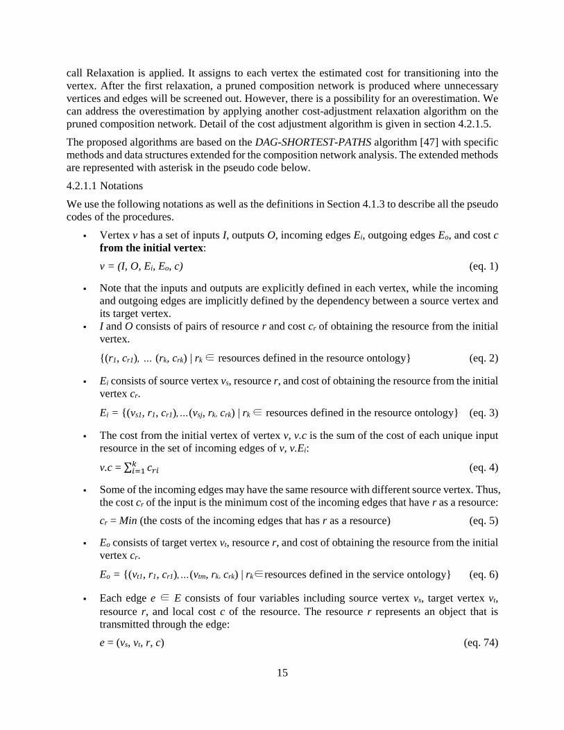
4.2.1.1 Notations

We use the following notations as well as the definitions in Section 4.1.3 to describe all the pseudo

codes of the procedures.

▪ Vertex v has a set of inputs I, outputs O, incoming edges Ei, outgoing edges Eo, and cost c

from the initial vertex:

v = (I, O, Ei, Eo, c) (eq. 1)

▪ Note that the inputs and outputs are explicitly defined in each vertex, while the incoming

and outgoing edges are implicitly defined by the dependency between a source vertex and

its target vertex.

▪ I and O consists of pairs of resource r and cost cr of obtaining the resource from the initial

vertex.

{(r1, cr1), … (rk, crk) | rk ∈ resources defined in the resource ontology} (eq. 2)

▪ Ei consists of source vertex vs, resource r, and cost of obtaining the resource from the initial

vertex cr.

Ei = {(vs1, r1, cr1),…(vsj, rk, crk) | rk ∈ resources defined in the resource ontology} (eq. 3)

▪ The cost from the initial vertex of vertex v, v.c is the sum of the cost of each unique input

resource in the set of incoming edges of v, v.Ei:

v.c = ∑ 𝑐𝑟𝑖𝑘𝑖=1 (eq. 4)

▪ Some of the incoming edges may have the same resource with different source vertex. Thus,

the cost cr of the input is the minimum cost of the incoming edges that have r as a resource:

cr = Min (the costs of the incoming edges that has r as a resource) (eq. 5)

▪ Eo consists of target vertex vt, resource r, and cost of obtaining the resource from the initial

vertex cr.

Eo = {(vt1, r1, cr1),…(vtm, rk, crk) | rk∈resources defined in the service ontology} (eq. 6)

▪ Each edge e ∈ E consists of four variables including source vertex vs, target vertex vt,

resource r, and local cost c of the resource. The resource r represents an object that is

transmitted through the edge:

e = (vs, vt, r, c) (eq. 74)

16

The pseudo code below shows the overall procedure of the composition network pruning and cost

estimation method using the notation.

COMPOSITION-NETWORK-PRUNING-AND-COST-ESTIMATION (RI, RG)

1 CN = GENERATE-COMPOSTION-NETWORK (RI, RG)

2 CN = TOPOLOGICAL-SORTING* (CN)

3 CN = VERTEX-INITIALIZATION* (CN)

4 for each vertex u in CN, taken in topologically sorted order

5 for each outgoing edges eo ∈ u.Eo

6 RELAXATION* (eo)

7 for each vertex u in CN, taken in topologically sorted order //pruning step

8 if u.c = ∞ then remove u and all its edges from CN

9 for each vertex u in CN, taken in topologically sorted order

10 for each outgoing edges eo ∈ u.Eo

11 COST-ADJUSTMENT* (eo)

4.2.1.2 Topological sorting

The topological sorting orders all the vertices linearly. Suppose that the composition network has

an edge (v1, v2). Then, v1 appears before v2 in the order after the topological sorting. One issue in

the topological sorting is that if the graph contains a cycle, then linear ordering of the vertices is

not possible. Therefore, we have to check whether the composition network contains a cycle. The

cycle detection can be done by the depth first search. A directed graph is acyclic if and only if a

depth-first search of the graph yields no back edges. If the graph contains a cycle, then we have to

make the composition network acyclic through the CREATE-STRONGLY-CONNECTED-

VERTEX method as described in [44]. Figure 7 below shows the result of the topological sorting

on the CN presented in the Figure 5.

TOPOLOGICAL-SORTING* (CN)

1 while (DEPTH-FIRST-SEARCH(CN)) {

2 If cycle detected // ‘back’ edge found

3 CN’ = CREATE-STRONGLY-CONNECTED-VERTEX (CN)

4 return TOPOLOGICAL-SORTING* (CN’)

5 Else

6 as each vertex is finished, insert it onto the front of a linked list

7 return the linked list of vertices }

17

Figure 7. Topologically sorted CN.

4.2.1.3 Vertex initialization

In this step, the costs in the input set, and in the incoming/outgoing edges of the vertex are

initialized following the pseudo code below. The initial vertex will have 0 as a cost, while others

are initialized with ∞. Figure 8 shows the result of the vertex initialization. The white boxes in the

bottom represent the cost of each corresponding vertex above.

VERTEX-INITIALIZATION* (CN, vI) // vI is the initial vertex

1 for each vertex v ∈ CN.V

2 for each vertex v’ ∈ CN.Adj[v] //Adj[v] is adjacent vertices of v in the linked list

3 set Eo in v and set Ei in v’

4 v.c = ∞

5 for each pair of resource r and its cost cr in the Ei

6 cr = ∞

5 for each pair of resource r and its cost cr in the Eo

6 cr = local cost of r from (eq. 5)

7 vI.c = 0

Figure 8. CN with the Vertex Initialization

18

4.2.1.4 Relaxation

The algorithm for composition network pruning and cost estimation uses the relaxation technique.

Each vertex maintains an upper bound of the cost from source vertex. The upper bound of the cost

is represented as ct. The ct of each vertex has been initialized as ∞ in the vertex initialization step.

The relaxation on an edge (u, v) checks whether the cost to v can be improved by going through u.

If the cost can be improved, then ct of v is updated. The details of the checking and updating

procedures are described in the following pseudo code.

RELAXATION* (eo)

1 Look up e ∈ E using eo.vt and eo.r

2 vs = e.vs, vt = e.vt

3 cnew = vs.c + eo.c

4 Get cost cr of the resource in vt.Ei using eo.r as a key

5 if cnew < cr then update cr = cnew in vt.Ei and update vt.c in eq. 1 using new cr via eq. 4.

Figure 9 below illustrates the result of the relaxation assuming the local cost of every resource is

1. The number in the white boxes represents the cost from the initial vertex to each vertex. There

is one vertex that has ∞ as a cost. Thus, the vertex as well as the edges of the vertex are eliminated

in the pruning step. Figure 10 shows the composition network left before the cost adjustment is

applied.

Figure 9. Result of the relaxation

19

Figure 10. Result of composition network pruning

4.2.1.5 Cost-adjustment

The resulting cost of each vertex in the previous section may be overestimated, specifically when

there are overlaps between paths. For example, let’s take a look at the illustration shown in Figure

11. Once again assuming that the local costs of all edges are 1. There are three paths from the start

vertex to the end vertex. For Object 7, there exists only one path while for Object 6, there are two

different paths. The minimum cost path for Object 6 is Path 3 that costs 3. Since there is only one

path for Object 7, if we just aggregate the minimum cost paths, then Path 2 and Path 3 will be

chosen, and the total cost would be 7. However, we can reduce the total cost to 6 by choosing Path

1 instead of Path 3 even though the cost of the Path 1 is greater than the Path 3, because Path 1

and Path 2 overlap. Thus, the cost of getting to the End vertex by the relaxation procedure was

overestimated. In order to avoid the overestimation in the example, the cost up to Service B should

be shared by Service C and D. That is, the cost of the shared path should not be added in both of

the branching paths.

Figure 11. Cost over estimation when branches exist.

To address this issue, the following cost-adjustment method is proposed. The cost-adjustment

divides the cost up to the precedent vertex by the degree of the outgoing edges when relaxing the

adjacent vertices of the precedent vertex.

20

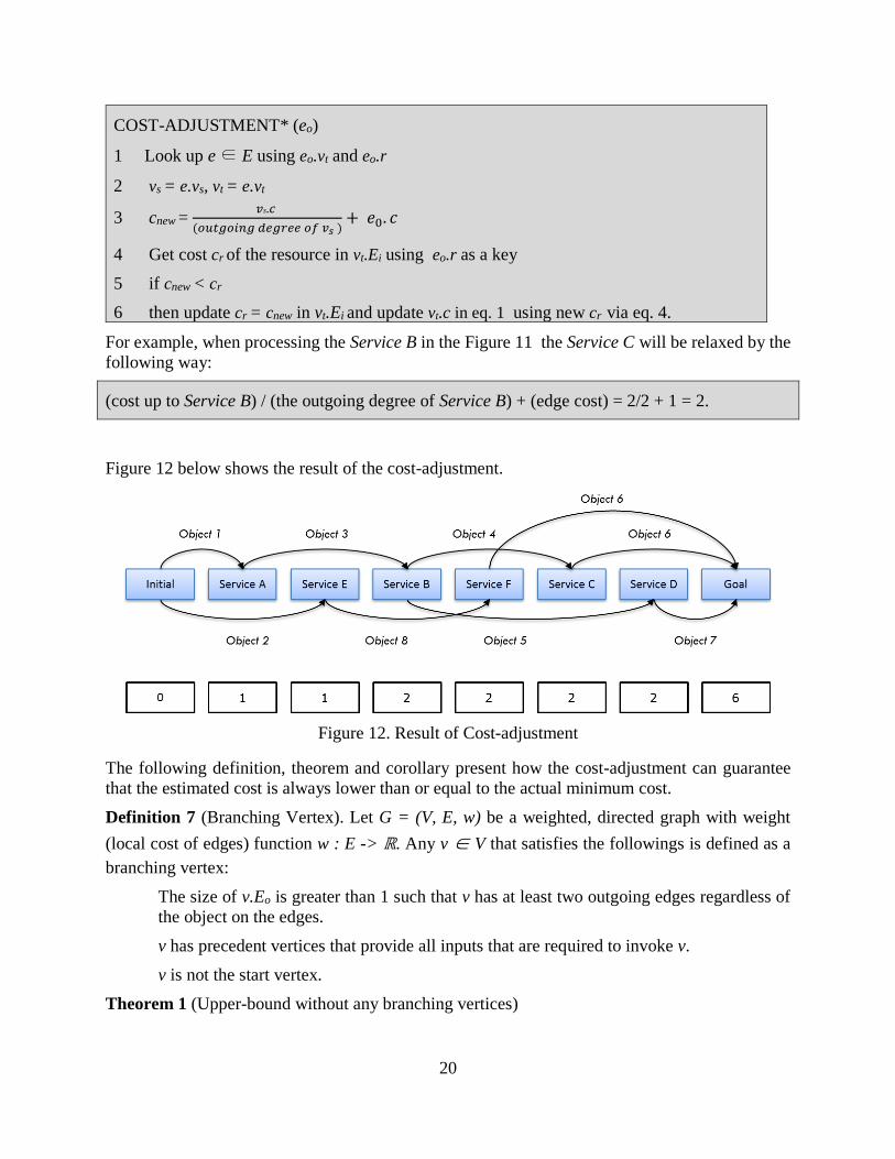
COST-ADJUSTMENT* (eo)

1 Look up e ∈ E using eo.vt and eo.r

2 vs = e.vs, vt = e.vt

3 cnew = 𝑣𝑠.𝑐

(𝑜𝑢𝑡𝑔𝑜𝑖𝑛𝑔 𝑑𝑒𝑔𝑟𝑒𝑒 𝑜𝑓 𝑣𝑠 )+ 𝑒0. 𝑐

4 Get cost cr of the resource in vt.Ei using eo.r as a key

5 if cnew < cr

6 then update cr = cnew in vt.Ei and update vt.c in eq. 1 using new cr via eq. 4.

For example, when processing the Service B in the Figure 11 the Service C will be relaxed by the

following way:

(cost up to Service B) / (the outgoing degree of Service B) + (edge cost) = 2/2 + 1 = 2.

Figure 12 below shows the result of the cost-adjustment.

Figure 12. Result of Cost-adjustment

The following definition, theorem and corollary present how the cost-adjustment can guarantee

that the estimated cost is always lower than or equal to the actual minimum cost.

Definition 7 (Branching Vertex). Let G = (V, E, w) be a weighted, directed graph with weight

(local cost of edges) function w : E -> ℝ. Any v ∈ V that satisfies the followings is defined as a

branching vertex:

The size of v.Eo is greater than 1 such that v has at least two outgoing edges regardless of

the object on the edges.

v has precedent vertices that provide all inputs that are required to invoke v.

v is not the start vertex.

Theorem 1 (Upper-bound without any branching vertices)

21

Let G = (V, E, w) be a Composition Network. Assume that the graph is relaxed by

RELAXATION*. Let G’ = (V’, E’, w) be the minimum cost solution graph of G that has s ∈ V’ as

the start vertex and v ∈ V’ as the terminal vertex. Assume that G’ does not have any branching

vertex, then v.ct = δ(s, v) after the COST-ADJUSTMENT*, where v.ct is the estimated cost of G’

and δ(s, v) is the actual minimum cost of G’.

Proof

Assume that v has n inputs, where n ≥ 1. Then, δ(s, v) = c(sg1) + c(sg2) + … + c(sgn), where c(sgk)

is the cost of the minimum cost solution graph for the input k of v.

There is no overlapping vertices or edges between the solution graphs because G’ does not have

any branching vertex. Thus, taking the minimum cost solution graph for each input of v always

guarantees the total minimum cost of v as the RELAXATION method does. Since there is no

branching vertex, COST-ADJUSTMENT* is exactly the same with the RELAXATION. Thus, v.ct

= δ(s, v).

Theorem 2 (Upper-bound with one branching vertex)

Let G = (V, E, w) be a Composition Network. Assume that the graph is relaxed by

RELAXATION*. Let G’ = (V’, E’, w) be the minimum cost solution graph of G that has s ∈ V’ as

the start vertex and v ∈ V’ as the terminal vertex. Assume that G’ has only one branching vertex u

∈ V’ and u has n outgoing edges, where n > 1. Then, v.ct < δ(s, v) after the COST-

ADJUSTMENT*, where v.ct is the estimated cost of G’ and δ(s, v) is the actual minimum cost of

G’.

Proof

Since there is no branching vertices in the precedent vertices of u, δ(s, u) = u.ct by Theorem 1.

Let G’’(V’’, E’’, w) be the minimum cost sub-solution graph of G’ that has s as the start vertex and

u as the terminal vertex. Then, E’’ ⊂ E’ and we can represent δ(s, v) by the following.

δ(s, v) = (the sum of the weights on ∀ e’ ∈ E’’) + X, where X is the sum of the weights

on ∀ e ∈ E’ – E’’ = δ(s, u) + X

After COST-ADJUSTMENT*, add 𝑢.𝑐𝑡

𝑛 to the weights of each outgoing edges of u and set 0 for ∀

e’ ∈ E’’. Let Eo be the set of the outgoing edges of u with n members.

If (∀ e ∈ Eo ) ∈ E’, then

v.ct = (𝑢.𝑐𝑡

𝑛) * n + X = u.ct + X = δ(s, u) + X = δ(s, v)

Else if (∃ e ∈ Eo ) ∈ E’, then

22

v.ct = (𝑢.𝑐𝑡

𝑛) * k + X , where k < n

< u.ct + X = δ(s, u) + X = δ(s, v)

Thus, v.ct ≤ δ(s, v)

Theorem 3 (Upper-bound with multiple branching vertices)

Let G = (V, E, w) be a Composition Network. Assume that the graph is relaxed by

RELAXATION*. Let G’ = (V’, E’, w) be the minimum cost solution graph of G that has s ∈ V’ as

the start vertex and v ∈ V’ as a terminal vertex. Then, v.ct ≤ δ(s, v) after the COST-

ADJUSTMENT*, where v.ct is the estimated cost of G’ and δ(s, v) is the actual minimum cost of

G’, and this invariant is maintained over any number of branching vertices in G’.

Proof

We prove the invariant v.ct ≤ δ(s, v) by induction over the number of branching vertices in G’. Let

the number of branching vertices in G’ be k. For the basis (k = 1), v.ct ≤ δ(s, v) is certainly true by

Theorem 2.

For the inductive step, consider there are n branching vertices in G’. By the inductive hypothesis,

v.ct ≤ δ(s, v) for all the number of branching vertices equal or less than n in G’.

Let Gn+1 = (Vn+1, En+1, w) be the minimum cost sub-solution graph of G’ that has s as the start

vertex and un+1 as the terminal vertex, where un+1 is the last branching vertex in topological order

in G’. Let U = {u1, …, un} be other branching vertices in G’.

If (∀ u ∈ U ) Vn+1 , then un+1 does not have any precedent branching vertices. Thus, v.ct ≤ δ(s,

v) by Theorem 2.

If (∃ u ∈ U ) ∈ Vn+1, let um be the last branching vertex in Gn+1 where 1 ≤ m ≤ n. Since Gn+1

has the number of branching vertices equal or less than n, by the inductive hypothesis, un+1.ct ≤

δ(s, un+1).

Since En+1 ⊂ E’, we can represent δ(s, v) by the following.

δ(s, v) = (the sum of the weights on ∀ e’ ∈ En+1) + X, where X is the sum of the weights

on ∀ e ∈ E’ – En+1.

= δ(s, un+1) + X

≥ un+1.ct + X

After COST-ADJUSTMENT* on un+1, add 𝑢𝑛+1.𝑐𝑡

𝑗 to the weights of each outgoing edges of un+1,

where j is the outgoing degree of un+1 and set 0 for ∀ e ∈ En+1. Let Eo be the set of the outgoing

edges of un+1.

If (∀ e ∈ Eo ) ∈ E’, then

23

v.ct = (𝑢𝑛+1.𝑐𝑡

𝑗) * j + X = un+1.ct + X ≤ δ(s, v)

Else if (∃ e ∈ E0 ) ∈ E’, then

v.ct = (𝑢𝑛+1.𝑐𝑡

𝑗) * k + X , where k < j

< un+1.ct + X ≤ δ(s, v)

Thus, the invariant is maintained.

The following corollary proves that the estimated cost resulting from the cost-adjustment process

is an admissible heuristic for searching AND/OR graph that is converted from a given CN. Thus,

the estimated cost can be used as a heuristic function for the search algorithm in section 4.2.2.

Corollary 1

The estimated cost resulting from the cost-adjustment process is an admissible heuristic for

AND/OR graph search.

Proof

An admissible heuristic is used to estimate the cost of reaching the goal state in an informed search

algorithm. In order for a heuristic to be admissible to the search problem, the estimated cost must

always be lower than or equal to the actual cost of reaching the goal state [43]. By the Theorem 1,

2, 3, the estimated cost is always lower than or equal to the actual cost. Thus, the estimated cost

resulting from the cost-adjustment process is an admissible heuristic.

4.2.2 Transformation to AND/OR graph

After the composition network pruning and cost estimation, the AND/OR graph conversion

method defined in section 4.1.2 is applied to the composition network. Figure 13 below shows the

transformed AND/OR graph from CN in Figure 12. Each AND vertex has an estimated cost that

is represented in the parenthesis.

24

Figure 13. Resulting AND/OR graph.

4.2.3 Minimum cost subgraph search algorithm

Nilsson [45] introduced the AND/OR graph, or A/O graph for short, and A/O graph search problem

for the first time, and since then various types of AND/OR graph search methods have been

proposed.

AND/OR graph search algorithms can be categorized into explicit-graph search and implicit-graph

search methods. The explicit-graph search uses an explicit data representation for the vertices and

edges of an AND/OR graph, while the implicit graph search uses rules to represent them. AO* is

an example of an implicit-graph search method [46].

AND/OR graph search methods can also be classified as admissible and inadmissible. While

admissible algorithms guarantee that an optimal solution will be found, if one exists, inadmissible

algorithms cannot guarantee that the solution found is an optimal solution. Our objective is to

develop admissible search method to find the minimum cost solution graph beginning from the

start vertex and leading to the terminating vertex. In the previous section, the composition network

pruning and cost estimation was a kind of implicit-graph search, while the AND/OR graph search

in this section is a kind of explicit-graph search, because we already have a set of candidate vertices

with explicit relations between the vertices and the estimated costs.

In our algorithm, notations used in Mahanti and Bagchi [47] are adopted as follows.

▪ G is the entire problem graph that results from the node network pruning.

▪ All vertices u in G has a finite set of successors S(u).

▪ h’(u) is an estimated cost at vertex u. This estimate will be used to guide the search and

reduce the number of expanded vertices.

25

▪ All edge (u, v) in G has a fixed cost c(u, v) >= 0 (this is the weight on the edge).

▪ P(u) denotes the set of predecessors of vertex u. For any vertex u in G, D(u) denotes a

solution graph with root u.

▪ The subgraph of G that is generated up to a certain point is called the explicit graph G’.

▪ A cost function h(v, G) on each vertex v in G is defined as follows:

- h(v, G) = lower bound {h(v, D(v)) | D(v) is a solution graph with root v in G}, where,

for a node u in D(v),

▪ h(u, D(u)) = 0, if u is a terminating vertex

▪ h(u, D(u)) = c(u, u’) + h(u’, D(u’)), if u is an OR vertex and u’ is v’s

immediate successor in D(u)

▪ h(u, D(u)) = ∑ (𝑐(𝑢, 𝑣𝑖) + ℎ(𝑣𝑖 , 𝐷(𝑣𝑖)))𝑘𝑖=1 , if u is an AND vertex with

immediate successors v1, v2, …, vk in D(u)

Our AND/OR graph search algorithm proceeds in a top-down fashion, where each vertex

expansion step is followed by a bottom-up cost revision like all AO algorithms [46]. The following

pseudo code describes the procedure of our algorithm. The minimum cost solution subgraph

consists of vertices labeled SOLVED after the algorithm exits.

SSCA-AND/OR-Graph-Search (G, s) // G is an AND/OR graph and s is a start vertex

1 If s is a terminal vertex, Then label s SOLVED

2 create G’ and add s to G’

3 While s is not SOLVED

4 choose any unsolved successor vertex u below s; expand u generating all its

successors into S(u);

5 Add u to G’

6 for each v ∈ S(u) not in G’

7 add v to G’

8 If v is a terminal vertex, label it SOLVED

9 Else compute h(v)

10 If h(v) > h’(v), BREAK

11 for each v ∈ S(u) in G’

12 recompute the costs of all predecessors in P(v) assuming h(v) = 0

13 for any v ∈ S(u)

14 If v is AND vertex and v has immediate predecessors other than S(u),

15 Then recompute costs of all predecessors in P(v) assuming h(v) = 0

16 Clear the SOLVED labels

26

17 Recompute the costs of immediate successor vertices of s, and label all vertices in

the minimum cost subgraph as SOLVED

18 If a terminal vertex is in G’, Then label s SOLVED

The outer loop of the algorithm implements the top-down growth of G’, while the inner loop carries

out the bottom-up cost revision. The estimated costs are revised from the expanded vertex up along

marked edges as well as other edges if there exists an AND vertex on the path. This revision

process may change the cost of the successor vertices below the start vertex that may leads to an

alternative, more promising paths.

The procedure is similar to the AO* algorithm [ref]. The main difference is the cost revision

process. Like AO* algorithm, our algorithm also propagates its new cost back up through the graph,

if the current vertex has been labeled SOLVED or its cost was just changed. In addition to that, if

the current path reaches to the terminating vertex and there exist any AND vertex on the path that

has another predecessor path, then our algorithm updates the cost of the vertices on the other

predecessor path assuming the cost of the current AND vertex is 0. This cost revision process is

necessary, because what we try to achieve is to find a minimum cost subgraph, not just a path, and

there might be a shared path in a subgraph.

Mahanti and Bagchi [47] has proven that, if the cost estimation is admissible (i.e., h’(u) ≤ h(u, G),

∀ u ∈ G), then AO* like algorithms terminate by either finding a minimum-cost solution graph

rooted at s or else returning h(s) = ∞. In our case, once the AND/OR graph is obtained from the

composition network, there must be a solution because section 4.2.1.5 has already proven that our

cost-estimation is admissible, i.e., v.ct ≤ δ(s, v).

5. Experiment

In this section, we compare the performance of our Service Search and Composability Analysis

(SSCA) algorithm and other prominent existing AI planners in terms of effectiveness and

computational efficiency. We chose OptaPlanner (V6.0.1) and BlackBox (V4.5) for the

performance comparison.

The OptaPlanner is a lightweight, embeddable planning engine based on a constraint satisfaction

solver [48]. Since the OptaPlanner provides various optimization heuristics and algorithms, it

enables the performance comparison of our algorithm with various combinations of optimization

heuristics. Throughout the experiments, Tabu Search [49], Simulated Annealing [50], and Hill

Climbing [51] were used as optimization heuristics and algorithms for the constraint satisfaction.

Blackbox is a planning system that combines best features of Graphplan [31], SATPLAN [31, -52],

and new randomized systematic search engines. Blackbox converts problems described in STRIPS

into Boolean satisfiability (SAT) problems, and then solves the problems with existing

satisfiability engines [53]. The front-end of Blackbox employs the Graphplan system [31] and for

the SAT problem, Blackbox applies the local-search SAT solver such as Walksat [52] and Satz

[55].

Two evaluation metrics were used in the experiments including execution time and total cost of a

solution. The execution time is to measure how long each algorithm takes to find a solution. The

27

time unit in this experiment is millisecond. The total cost of a solution is to measure the quality of

the solution obtained. The total cost is the sum of the weights on edges in a solution.

The experiments were performed on Mac OS X version 10.9.5 with 3.5 GHz Intel Core i7 and

8GB 1600 MHz DDR3 RAM.

The first experiment is to analyze the correlation between the number of vertices and the

performance of each planner. For this experiment, test data are randomly generated as follows.

▪ 50 different objects are generated for use as inputs and outputs of vertices.

▪ Each vertex has at least one and at most three inputs and outputs. The number of inputs

and outputs are randomly selected within the restriction.

▪ There is no duplication between inputs and outputs of each vertex.

▪ For each of the test data set, user’s initial condition, goal condition, and solutions are

created.

We have generated total 21 different sizes of test data set by varying the size of vertices as 10, 100

to 900, and 1,000 to 10,0005. Each test data set has 4 possible solutions and 1 optimal solution.

The optimal solution is a solution graph that has 3 vertices.

Table 1 and Figure 14 below show the result of the first experiment. The bold font in the table

represents the best performance and the underscore represents sub-optimal result. The number in

the parenthesis after the execution time shows the number of resulting vertices in the suboptimal

solution. It can be seen that SSCA and Blackbox outperform CSP-based methods. Figure 15 below

shows the performance comparison between SSCA and Blackbox. Blackbox produced suboptimal

solutions when the number of vertices is 200, 300, and 500.

Table 1. Execution times from the experiment by varying the number of vertices

# of

Vertices SSCA Blackbox

CSP

(Tabu)

CSP

(SA)

CSP

(HC)

10 0.002 0.007 0.037 0.032 0.027

100 0.004 0.013 0.089 0.078 0.05

200 0.013 0.02 (5) 0.079 0.094 0.19

300 0.024 0.026 (5) 0.093 0.091 0.297

400 0.003 0.004 0.098 0.134 0.148

500 0.055 0.047 (4) 0.096 0.138 0.187

5 Ten thousand service nodes may sound unrealistically large for a services composition problem in engineering

domain. However, a single service in the actual service implementation may need to be represented as multiple

services in the automatic services composition problems, for example, due to flexibility to process several input

formats, unit of measures, security mechanisms with different quality of service levels. This will increase the number

of nodes.

28

600 0.004 0.004 0.096 0.177 0.218

700 0.003 0.005 0.109 0.22 0.231

800 0.003 0.006 0.113 0.316 0.457

900 0.004 0.004 0.115 0.107 0.3

1000 0.002 0.005 0.115 0.161 0.215

2000 0.003 0.006 0.39 0.952 0.489

3000 0.002 0.005 0.415 0.576 0.409

4000 0.004 0.007 0.489 0.445 0.85

5000 0.005 0.007 0.603 1.147 0.966

6000 0.005 0.008 0.601 0.34 1.542

7000 0.003 0.008 0.917 1.887 0.434

8000 0.006 0.01 1.237 0.926 1.001

9000 0.005 0.009 0.659 0.432 1.355

10000 0.006 0.009 0.664 2.351 0.59

The execution time in both SSCA and Blackbox is quite steady regardless of the number of vertices

while the execution time in CSP-based planner tends to increase in proportion to the number of

vertices. That is mainly due to the fact that both the SSCA and Blackbox identify solution

candidates in the forward search phase by expanding a graph from the initial states until all goal

states appear. Since, in this first experiment, all the test data set has a small number of vertices in

the solution graph and also each vertex has at most 3 outputs, the number of the solution candidates

is small, thus those are identified quickly and that significantly reduce the entire search space. On

the other hand, in the case of CSP-based planners, there is no such pruning process, thus the

execution time increases as the number of vertices is increased.

29

Figure 14. Performance comparison by varying the number of vertices

Figure 15. Performance comparison between SSCA and Blackbox

From the result of the first experiment, we observe that the number of vertices is not critical for

both SSCA and Blackbox. As described in the result of the first experiment, both the SSCA and

Blackbox identify solution candidates in the forward search phase by expanding a graph from the

initial states until all goal states appear. If each vertex has more outgoing degree, then more vertices

30

are expanded in the forward search phase and it would require longer search time. Thus, the second

experiment is to analyze the correlation between the outgoing degree of vertices and the

performance of each planner.

For the second experiment, test data are randomly generated as follows.

▪ 200 different objects are generated for use as inputs and outputs of vertices.

▪ 13 different test data sets are generated by varying the outgoing degree of vertices as 1, 2,

3, 4, 5, 10, 15, 20, 25, 30, 35, 40, and 45. Outgoing degree 10 means that each vertex has

10 outputs.

▪ Each vertex has only one input.

▪ There is no duplication between inputs and outputs of each vertex. For example, if a vertex

has an object as an input, then that object cannot be used as an output.

▪ For each of the test data set, user’s initial condition, goal condition, solutions are created.

▪ Each test data set has a total of 1,000 vertices.

▪ Each test data set has 4 possible solutions and 1 optimal solution. The optimal solution is

a solution graph that has 3 vertices

Table 2 and Figure 16 below show the result of the second experiment. Same as the Table 1, the

bold font in the table represents the best performance and the underscore represents sub-optimal

result. The number in the parenthesis after the execution time shows the number of resulting

vertices in the suboptimal solution. It can be seen that SSCA outperforms the other methods. The

Blackbox produced suboptimal solutions when the outgoing degree is 2 and 3. And, the Blackbox

didn’t work at all when the outgoing degree is greater than 3.

Table 2. Execution time from the experiment by varying the outgoing degree of vertices

Outgoing

Degree SSCA Blackbox

CSP

(Tabu)

CSP

(SA)

CSP

(HC)

1 0.002 0.002 0.161 0.183 0.262

2 0.024 0.011(4) 0.292 0.173 0.402

3 0.032 0.04(4) 0.396 0.265 0.139

4 0.041 - 0.467 0.369 0.456

5 0.043 - 0.469 0.104 1.251

10 0.124 - 0.968 0.832 0.561

15 0.176 - 0.895 1.986 1.725

20 0.201 - 1.496 1.311 0.824

25 0.285 - 2.783 1.703 0.531

30 0.368 - 2.547 2.336 1.878

35 0.381 - 0.576 3.886 2.285

40 0.433 - 1.777 4.406 11.152

31

45 0.462 - 2.837 4.637 3.212

Figure 16. Performance comparison by varying the outgoing degree of vertices

6. Discussion

The two experiments above show that SSCA is capable of solving the service search and

composition problems better than other prominent methods compared in terms of performance and

scalability. Specifically, the SSCA shows a significantly better performance than those other

methods when the number of vertices is large, particularly with over a thousand vertices, and the

composition network is dense with tens of outgoing degrees. The Blackbox performs well but does

not converge when the outgoing degree is greater than 3. The CSP-based planners require much

more execution time than the SSCA. The experiments show evidences that these other methods are

not as scalable as SSCA.

The CSP-based planners always find optimal solutions in the experiments, because the time bound

was not set. However, the CSP-based planners may not find the optimal solution, if the time bound

was set lesser than the execution time in the Table 1 and Table 2. It is important to note that the

computational time of SSCA did not grow exponentially when the number of vertices and the

density increase; hence SSCA has a strong scalability.

7. Conclusion

This research developed a computer-aided services search and composition methods for an open

cloud services marketplace environment. There are two main research contributions in this paper.

First, a model for formally representing a service was proposed. In this vein, our analysis of

previous works in function representation theory and requirement engineering concludes that 1)

both service functional and non-functional characteristics are essential to considered in services

composition to achieve functional goal while maximize qualities and minimize costs; 2) functional

characteristics can be device-centric or environment-centric and can be modeled as input, output,

pre-condition, post-condition, and behavioral properties; and 3) non-functional characteristics can

be generalized as qualities. Both behavioral properties and qualities can be commonly represented

as an expression that is a fixed value, a range or equation over some parameters.

32

The second research contribution is the framework for Service Search and Composability Analysis

(SSCA). SSCA framework include 1) procedure to represent a services composition problem as a

composition network; 2) a procedure to reduce and transform the composition network into an

AND/OR graph with cost estimations; and 3) a specialized planning algorithm to find the

minimum cost solution subgraph using the cost estimation as the heuristic. A proof was provided

to show that the proposed cost estimation is an admissible heuristic; and hence, the SSCA heuristic-

based planning algorithm will always return a minimum cost solution subgraph, if one exists, per

the proof provided by a prior research. Simulation experiments were conducted; and the results

affirmed the proof and demonstrated the strong scalability characteristics compared to other

prominent planners.

In terms of future work, more complex cost scheme should be considered for characterizing

behavioral properties and qualities such as duration, reputation, reliability, and availability and

their interactions when services are composed (e.g., cross-sale and volume discount). In the current

work, these characteristics are constrained to be represented as a consolidated, static cost for each

service.

Reference

1. Kulvatunyou B, Ivezic N, Srinivasan, V. (2016). On architecting and composing engineering

information services to enable smart manufacturing. Journal of Computing and Information

Science in Engineering, 16(3), 31002.

2. Davis, J., Edgar, T., Graybill, R., Korambath, P., Schott, B., Swink, D., & Wetzel, J. (2015).

Smart manufacturing. Annual Review of Chemical and Biomolecular Engineering, 6, 141–

160.

3. W3C - World Wide Web Consortium (2001), Web Services Description Language (WSDL)

1.1, March 15 2001, available online at http://www.w3.org/TR/wsdl/.

4. Open API Specification version 3.0, Released July, 2017. Available online at

https://www.openapis.org/.

5. Lin, S.Y., Lin, G.T., Chao, K.M. and Lo, C.C. (2012) ‘A cost effective planning graph

approach for large scale Web service composition’, Mathematical Problems in Engineering.

Article ID. 783476, pp.21.

6. Yan, Y., Chen, M., & Yang, Y. (2012, March). Anytime QoS optimization over the PlanGraph

for web service composition. In Proceedings of the 27th Annual ACM Symposium on Applied

Computing (pp. 1968-1975). ACM.

7. Hatzi, O., Vrakas, D., Bassiliades, N., Anagnostopoulos, D., & Vlahavas, I. (2013). The

PORSCE II framework: Using AI planning for automated semantic web service composition.

The Knowledge Engineering Review, 28(02), 137-156.

8. Nils J. Nilsson. ―Artificial Intelligence: a new synthesis". Morgan Kaufmann, San Francisco,

CA, USA, 2001.

9. Oh, S. C., Lee, D., & Kumara, S. R. (2008). Effective web service composition in diverse and

large-scale service networks. Services Computing, IEEE Transactions on, 1(1), 15-32.

33

10. W3C – World Wide Web Consortium (2004), OWL-S: Semantic Markup for Web Services,

November 22, 2004, available online at http://www.w3.org/Submission/2004/SUBM-OWL-

S-20041122/, accessed July 2018.

11. W3C – World Wide Web Consortium (2007), Semantic Annotations for WSDL and XML

Schema, August 28, 2007, available online at http://www.w3.org/TR/sawsdl/

12. W3C – World Wide Web Consortium (2005), Web Service Modeling Ontology (WSMO),

June 3, 2005, available online http://www.w3.org/Submission/WSMO/

13. Kulvatunyou, B., Wallace, E.K., Kiritsis, D., Smith, B.S., Will, C. (August 2018). The

Industrial Ontologies Foundry Proof-of-Concept. In Proc. of Intl. Conf. on Advances in

Production Management Systems (APMS 2018), Seoul, South Korea.

14. Kulvatunyou, B. and Ivezic, N. (June, 2002). Semantic Web for Manufacturing Web Services,

International Symposium on Manufacturing and Applications (ISOMA), Orlando, Florida.

15. Jang, J., Jeong, B., Kulvatunyou, B., Chang, J., and Cho, H. Discovering and Integrating

Distributed Manufacturing Services with Semantic Manufacturing Capability Profiles,

International Journal of Computer-Integrated Manufacturing, 21(6), pp 631-646, 2008.

16. Barkmeyer, E. and Kulvatunyou, B. An Ontology for the e-Kanban Business Process, NIST

Internal Report 7404, 2007.

17. Ameri, F., & Dutta, D. (2006, January). An upper ontology for manufacturing service

description. In ASME 2006 international design engineering technical conferences and

computers and information in engineering conference (pp. 651-661). American Society of

Mechanical Engineers.

18. Witherell, P., Krishnamurty, S., & Grosse, I. R. (2007). Ontologies for supporting engineering

design optimization. Journal of Computing and Information Science in Engineering, 7(2), 141-

150.

19. Glinz, M. (2007, October). On non-functional requirements. In Requirements Engineering

Conference, 2007. RE'07. 15th IEEE International (pp. 21-26). IEEE.

20. Suzanne, R. and James, R. (1999) Mastering the Requirements Process, Addison-Wesley,

Boston.

21. Sommerville, I. (2004) Software Engineering, International Computer Science Series,

AddisonWesley, Boston.

22. Anton, A.I. (1997) Goal Identification and Refinement in the Specification of Information

Systems. PhD Thesis, Georgia Institute of Technology.

23. Davis, A. M. (1993). Software requirements: objects, functions, and states. Prentice-Hall, Inc.

24. IEEE Computer Society. Software Engineering Standards Committee, & IEEE-SA Standards

Board. (1998). IEEE Recommended Practice for Software Requirements Specifications.

Institute of Electrical and Electronics Engineers.

25. Chittaro, L., & Kumar, A. N. (1998). Reasoning about function and its applications to

engineering. Artificial intelligence in engineering, 12(4), 331-336.

26. Chakrabarti, A. (1998, July). Supporting two views of function in mechanical designs. In

Proceedings 15th national conference on artificial intelligence, AAAI (Vol. 98, pp. 26-30).

34

27. Chakrabarti, A., & Bligh, T. P. (2001). A scheme for functional reasoning in conceptual

design. Design Studies, 22(6), 493-517.

28. Deng, Y. M. (2002). Function and behavior representation in conceptual mechanical design.

AI EDAM, 16(05), 343-362.

29. Chandrasekaran, B., & Josephson, J. R. (2000). Function in device representation. Engineering

with computers, 16(3-4), 162-177.

30. Chandrasekaran, B. (2005). Representing function: relating functional representation and

functional modeling research streams. AIE EDAM, 19(02), 65-74.

31. Blum, A. L., & Furst, M. L. (1997). Fast planning through planning graph analysis. Artificial

intelligence, 90(1), 281-300

32. Kautz, H. A., & Selman, B. (1992, August). Planning as Satisfiability. In ECAI (Vol. 92, pp.

359-363).

33. Do, M. B., & Kambhampati, S. (2001). Planning as constraint satisfaction: Solving the

planning graph by compiling it into CSP. Artificial Intelligence, 132(2), 151-182.

34. Vossen, T., Ball, M., Lotem, A., & Nau, D. (2000). Applying integer programming to AI

planning. The Knowledge Engineering Review, 15(01), 85-100.

35. Sirin, E. (2004). Automated composition of web services using AI planning techniques.

(Master’s thesis), Department of Computer Science, University of Maryland.

36. Hashemian, S. V., & Mavaddat, F. (2005, January). A graph-based approach to web services

composition. In Applications and the Internet, 2005. Proceedings. The 2005 Symposium on

(pp. 183-189). IEEE.

37. Oh, S. C., On, B. W., Larson, E. J., & Lee, D. (2005, March). BF*: Web services discovery

and composition as graph search problem. In e-Technology, e174 Commerce and e-Service,

2005. EEE'05. Proceedings. The 2005 IEEE International Conference on (pp. 784-786). IEEE.

38. Zhang, R., Arpinar, I. B., & AlemanMeza, B. (2003, June). Automatic Composition of

Semantic Web Services. In ICWS (Vol. 3, pp. 38-41).

39. Bellman, R. (1956). On a routing problem (No. RAND-P-1000). RAND CORP SANTA

MONICA CA.

40. Ford Jr, L. R. (1956). Network flow theory (No. P-923). RAND CORP SANTA MONICA

CA.

41. Moore, E.F. (1957) ‘The Shortest Path Through a Maze’, Proceedings of an international

symposium on the theory of switching, Part II, pp.285-292.

42. E. Dikjstra (1968, March). A case against the GO TO statement. ACM 11, 366-371.

43. Balakrishnan, R. and Ranganathan, K. (2012) A Textbook of Graph Theory, Springer Science

& Business Media, New York, NY.

44. M. Henzinger, S. Krinninger, and V. Loitzenbauer. 2015. Finding 2-edge and 2-vertex strongly

connected components in quadratic time. In Proceedings of the 42nd International Colloquium

on Automata, Languages, and Programming. 713-724.

35

45. Nilsson, N. (1971) Problem Solving Methods in Artificial Intelligence, McGraw-Hill, New

York, NY.

46. E. Hansen and S. Zilberstein. LAO*: A heuristic search algorithm that finds solutions with

loops. Artificial Intelligence, 129:35–62, 2001.

47. A. Mahanti, A. Bagchi, AND/OR graph heuristic search methods, J. ACM 32 (1) (1985) 28–

51.

48. OptaPlanner, available online at http://www.optaplanner.org//, accessed May 2018.

49. Glover, F. (1989). Tabu search-part I. ORSA Journal on computing, 1(3), 190-206.

50. Davis, L. (1987) Genetic Algorithms and Simulated Annealing, Pitman, London.

51. Davis, A.M. (1993) Software Requirements: Ob-jects, Functions, and States, Prentice Hall,

Englewood Cliffs, NJ.

52. Selman, B., Kautz, H. A., & Cohen, B. (1994, October). Noise strategies for improving local

search. In AAAI (Vol. 94, pp. 337-343).

53. Fikes, R. E., & Nilsson, N. J. (1972). STRIPS: A new approach to the application of theorem

proving to problem solving. Artificial intelligence, 2(3), 189-208.

54. Selman, B., Kautz, H. A., & Cohen, B. (1994, October). Noise strategies for improving local

search. In AAAI (Vol. 94, pp. 337-343).

55. Li, C. M., & Anbulagan, A. (1997, August). Heuristics based on unit propagation for

satisfiability problems. In Proceedings of the 15th international joint conference on Artifical

intelligence Volume 1 (pp. 366-371). Morgan Kaufmann Publishers Inc..