A Gosset G Flouriot Report - University of Washington

Ensign GOSSET Ensign FLOURIOT

AAcckknnoowwlleeddggmmeennttss It is a pleasure to thank all those who made this study possible, especially including the following persons. We are heartily thankful to our supervisor, Dr Alberto Aliseda, whose encouragement, guidance and support from the initial to the final level, enabled us to develop an understanding of the subject. We also want to thank Mr Teymour Javaherchi, our tutor, who has made available his support in a number of ways, especially at the beginning of the project, to learn about numerical and post treatment software, and then for all his advice. We owe to Mr Deniset a deep gratitude for his full support and all his advice about numerical methods and modeling. Lastly we would offer our regards to Mr Martineau Deputy Head of Studies of the French Naval Academy and Mr Billard, Head of Master department of the French Naval Academy. Thanks to their human qualities, they understood the importance of going on this project in the best conditions, and gave us their encouragements.


Key words: Marine Hydrokinetic Turbines – Wake – Array optimization – Energetic efficiency

OOppttiimmiizzaattiioonn ooff PPoowweerr EExxttrraaccttiioonn iinn aann aarrrraayy ooff MMaarriinnee HHyyddrrookkiinneettiicc TTuurrbbiinneess

Students : Ensigns A.GOSSET and G .FLOURIOT, EN 2008 Departments : Energy Engineering Department and Master Department Host institution of studies : Department of mechanical engineering, University of Washington – Seattle (WA), USA Director of research : Assistant Professor, A. Aliseda Tutor of project : Master Student T. Javaherchi Corresponding officer : LTCR Durand, Director of Studies Assistant

AABBSSTTRRAACCTT

The application of Horizontal Axis Marine Hydrokinetic Turbines to generate electricity is a new technology that promises to produce clean and renewable energy from a highly predictable source. There are significant scientific and technological challenges that need to be overcome before this technology can be deployed in a large scale. The most important issue that needs to be understood for this technology to be efficient is how the turbines in a large array will interact on each other. This is particularly difficult to investigate since array effects can not be investigated experimentally due to high costs and difficulties to obtain permits. Consequently computational simulation has been selected as an efficient method to study these problems and provide a wealth of information to evaluate future turbine designs. The power extraction is investigated through a series of simple turbine arrangements where one turbine is located in the wake of another. The performance of the downstream turbine is analyzed and compared to the upstream one, used as a reference. The power, wake and velocity are studied as a function of downstream spacing. Thus, an optimum is evaluated as a trade-off between total power per unit length of the channel, cost of producing electricity and environmental impact.

RREESSUUMMEE

L’utilisation d’hydroliennes à axe horizontal pour générer de l’électricité est une technologie nouvelle qui permet la production d’énergie renouvelable à partir de sources connues. Néanmoins, des défis scientifiques et technologiques significatifs doivent être surmontés avant de déployer cette technologie à grande échelle. Pour être rentable, le plus important consiste à comprendre comment des turbines placées au sein d’un large réseau interagissent entre elles. Ceci est particulièrement complexe à mettre en œuvre expérimentalement, étant donnés les coûts financiers et l’obtention difficile d’autorisations. La simulation numérique est donc une alternative efficace au problème et peut fournir nombre d’informations afin d’évaluer la conception future des hydroliennes. La puissance extraite est ici examinée au travers de combinaisons simples, au sein de réseaux de turbines positionnées l’une derrière le sillage de l’autre. Les performances de la turbine en aval du courant sont analysées et comparées à celle de la première, faisant office de référence. La puissance, le sillage et la vitesse sont étudiés en fonction de l’espacement en aval. Une optimisation est donc expérimentée grâce à un compromis en la puissance totale par longueur d’unité d’un canal, le coût de la production électrique, et son impact environnemental.


French Naval Academy Ref : FYP MP 8

Optimization of Power Extraction in an array of Marine Hydrokinetic Turbines 1

GGlloossssaarryy

ABBREVIATIONS LIST OF NOTATION

ADM Actuator Disk Model Symbol Designation and Units

LHS Left Hand Side Scell Surface of the grid cell (m2)

MHK Marine Hydrokinetic Si Mean strain rate

QUICK Quadratic Upwind Interpolation for Convective Kinematics

U∞, V0 Free stream velocity (m.s-1)

V Local velocity (m.s-1)

NREL National Renewable Energy Laboratory V Average velocity (m.s-1)

NURBS Non-Uniform Rational Basis Splines Vc Centerline velocity (m.s-1)

RANS Reynolds-averaged Navier–Stokes Vcell Volume of the grid cell (m3)

SIMPLE Semi-Implicit Method for Pressure-Linked Equations

Vd Centerline velocity deficit (m.s-1)

Vtot Total velocity (m.s-1)

SST Shear-Stress Transport Vy y-velocity (m.s-1)

SRF Single Reference Frame

Vy/V0 Normalized velocity by the free stream velocity

SST Shear-Stress Transport W Width of the domain

UDF User Defined Functions

X/R Normalized x-coordinate by the radius

VBM Virtual Blade Model Y/R Normalized y-coordinate by the radius

LIST OF NOTATION Z/R Normalized z-coordinate by the radius

Symbol Designation and Units a Axial inductor factor

A1 Surface on the actuator disk (m2) c (r/R) Chord length

AOA / α Angle of attack (°) d Normalized distance by the radius

C2 Pressure jump coefficient (m-1) dtips Distance from the tips to a wall (R)

CD Drag coefficient k Turbulent kinetic energy (m2.s-2)

CL Lift coefficient lmesh Length of an edge to mesh

Cp Power coefficient p Pressure (Pa)

D Diameter (m) p1 Pressure on the actuator disk (Pa)

F1 Force of the flow on the actuator disk (N) p∞ Pressure on the upstream actuator disk (Pa)

FD Drag force (N) r Radial position from the center (m)

FL Lift force (N) u, v Velocity (m.s-1)

G Resolution of the mesh V Time average of the velocity (m.s-1)

pM& Momentum flow rate (kg.m-2.s-1) u1 Velocity on the actuator disk (m.s-1)

∞M& Momentum flow rate at the inlet (kg.m-2.s-1) u2 Velocity downstream of the actuator disk (m.s-1)

dM& Momentum deficit (kg.m-2.s-1) x Lateral coordinate direction (m)

Ma Mach number y Longitudinal coordinate direction (m)

Nb Number of blades z Vertical coordinate direction (m)

Nbi Number of interval counts for meshing Ε Decay rate velocity

P Power (kg.m2.s-3) ∆m Thickness of the media (m)

Pe Power extracted (kg.m2.s-3) ∆p Pressure drop (Pa)

Pemax Maximum power extracted (kg.m2.s-3) α Face permeability (m2)

Petotal Total power extracted (kg.m2.s-3) 1/α Viscous resistance coefficient (m-2)

Pideal Ideal power extracted by one turbine (kg.m2.s-3) ε Velocity deficit

Ptotal Total power available (kg.m2.s-3) η Efficiency

R Radius R=5.53m (m) µ Dynamic viscosity (kg.m-1.s-1)

Re Reynolds number ρ Density (kg.m-3)

S Surface (m2) ω Rotor speed (rpm)




TTaabbllee ooff ccoonntteennttss 1. INTRODUCTION: ................................................................................................................ 3

2. CONTEXT OF THE STUDY ................................................................................................ 4

2.1 Description of the turbine ........................................................................................................... 4

2.2 Problematic linked with arrays of turbines .............................................................................. 5

2.3. The Virtual Blade Model ........................................................................................................... 6

3. COMPUTATIONAL MODEL .............................................................................................. 8

3.1 Designing computational domains ............................................................................................. 8 3.1.1 Simple model, bases for building a mesh .............................................................................................. 8 3.1.2 Geometry of computational model and mesh ....................................................................................... 9 3.1.3 Designing a mesh for offset elements ................................................................................................. 10

3.2 Boundary conditions ................................................................................................................. 11 3.2.1 Constant velocity inlet ........................................................................................................................ 12 3.2.2 Non linear velocity inlet ...................................................................................................................... 12

3.3 Physical notions and elements (Navier-Stokes…) .................................................................. 14 3.3.1 Navier-Stokes equations ..................................................................................................................... 14 3.3.2 Turbulent flow .................................................................................................................................... 14 3.3.3 Governing equations: .......................................................................................................................... 15

3.4 Numerical methods and spatial discretization ........................................................................ 16 3.4.1 Turbulence model ............................................................................................................................... 16 3.4.2 Physical properties of the working fluid. ............................................................................................ 17 3.4.3 Solution methods ................................................................................................................................ 17 3.4.4 Solution initialization .......................................................................................................................... 17 3.4.5 Residuals monitor ............................................................................................................................... 17

4. IMPROVEMENT OF THE MODEL ................................................................................. 18

4.1 The Actuator Disk Model (ADM) ............................................................................................ 18

4.2 Analysis of the meshing sensitivity ........................................................................................... 23 4.2.1 Influence of the mesh refinement ........................................................................................................ 23 4.2.2 Mesh resolution between inlet and turbine ......................................................................................... 24 4.2.3 Influence of the domain width to turbine swept area .......................................................................... 26

5. RESULTS ............................................................................................................................. 28

5.1 Array of three turbines ............................................................................................................. 28 5.1.1Velocity contour and velocity profile .................................................................................................. 28 5.1.2 Velocity deficit and momentum deficit ............................................................................................... 30 5.1.3 Power and efficiency ........................................................................................................................... 32

5.2 Array of four turbines ............................................................................................................... 34 5.2.1 Velocity contour.................................................................................................................................. 34 5.2.2 Power and efficiency ........................................................................................................................... 36

5.3 Optimization of an array of turbines ....................................................................................... 37 5.3.1 Array of two turbines .......................................................................................................................... 37 5.3.2 Generalization of an array of turbine .................................................................................................. 39 5.3.3 Perspectives ........................................................................................................................................ 41 5.3.4 Limitations of the numerical model .................................................................................................... 41

6. CONCLUSION .................................................................................................................... 42

Appendixes ............................................................................................................................... 43

References ................................................................................................................................ 49




11.. IINNTTRROODDUUCCTTIIOONN:: The realization and development of clean and renewable energy is important for the future of power generation throughout the world, due the impact of fossil fuel use and global climate warming. Most of energy associated with natural resources comes from wind and water. Around the world, wind energy has taken up a big part of the current renewable energy market over the last twenty years, just because it is a relative mature industry with long term technology development. As seventy percent of the Earth's surface is covered with water, marine resources have a huge potential in energy generation. Marine energy is a recently considered source of renewable energy that includes power generation from tidal currents, ocean currents, and waves. The potential of power generation from marine tidal currents is sizable. The technology used to extract power from the wind and tidal current energy is similar for most proposed devices. The tidal energy derives its advantage from being highly predictable and available near population centers. In this study a Horizontal Axis Marine Hydrokinetic Turbine is used based on validated experimental parameters from a wind turbine. However, flow conditions studied are representative of tidal turbine, which differ significantly from wind turbines. The motivation for this study is to evaluate the feasibility of developing Marine Hydrokinetic Turbines in a large scale. But due to the high cost of experimental research, computational simulation is the most efficient method to evaluate future designs. The main objective of the present work is to carry out research on the optimization of power extracted in an array of Marine Hydrokinetic Turbines. Gathering several turbines in an array poses some constraints among which, the most important is the influence of the wake of upstream turbines that may interfere with downstream turbines, reducing the amount of energy produced. In order to achieve optimization of power extraction in an array of Marine Hydrokinetic Turbines, the extracted power by downstream turbines must be compared with the power extracted from upstream ones. Following the previous work in numerical methods by Mr Antheaume [1] and Mr Javaherchi [2], who compared several models to investigate the performance of single turbines, the Virtual Blade Model [3] is applied to explore performances of turbines in several arrangements. New meshes are designed to enable a numerical computation and the model is presented so that its limitations can be understood. Then, it is improved with the inclusion of the Actuator Disk Model to better represent the hub effect in the wake flow field, and the meshes are also optimized to gain in accuracy. Thus, the wake, the velocity and the extracted power can be analyzed as a function of distance downstream of the first turbine, in order to evaluate the total power extracted by an array of Marine Hydrokinetic Turbines. Due to the imparted time of the study, the through optimization of power extraction takes precedence over the study and evaluation of the consequences on sediment transportation, described in Appendix E, and offered as perspective to allow for a continuation of this study.




22.. CCOONNTTEEXXTT OOFF TTHHEE SSTTUUDDYY 2.1 Description of the turbine The geometry for the turbine used in this study is based on a horizontal-axis wind turbine. This turbine was tested by the NREL (National Renewable Energy Laboratory) in a wind tunnel located at the NASA Ames Research Centre, at Moffett Field in California. This provides optimum experimental validation for the methods used to investigate the array performance and environmental effects. Although there are differences in the design of MHK turbines with respect to wind turbines, associated with the different structural loading and the influence of cavitation in MHK, the study with the NREL Phase VI [4] serves as a baseline to identify the key phenomena to investigate and the right parameter range in which to study them. The turbine represented in Figure n°1, is a two bladed turbine, with a rotor radius of 5.53 meters long. In our experimental conditions the turbine is at 16.59 meters from the bottom of the domain. The parameters of the rotor are defined in the Virtual Blade Model (VBM), which is developed in Subsection 2.3 and imported in the software Fluent® as shown in Figure n°3. Using this, we will be able to understand wake and distance effects in some arrays of turbines. Those effects are the main issues where further understanding is needed to optimize the placement of each turbine, to extract power in the more efficient way possible, in balance with the other constraints described in the next Subsection 2.2.

Figure n° 1: Horizontal-axis wind turbine.




Figure n° 2: Interaction between geography, water depth, merchant traffic and implantation sites to experiment on MHK turbines in the vicinity of Seattle (WA) established with data from [13] and [14].

15 km Ferries traffic Merchant vessels traffic Main sites concerned by high speed

tidal currents ( 1.2 −≈ sm )[13] and [14]

2.2 Problematic linked with arrays of turbines In a tidal current channel, the kinetic energy flux results from the velocity of water through a cross section. It is expressed by the following equation (1) [5, Subsection 1.2., p7].

3

21

VSP ρ= (1)

where ρ is the density of water, S is the

surface of that section, and V is the average water velocity perpendicular to the channel, that is obtained by integrating the local velocities perpendicular to the channel V on the surface S [5, Subsection 1.2.2, p8]:

∫=S

dSVV (2)

In equation (1), as the velocity is a cubic term, it has the most important influence on the kinetic energy flux, and consequently, on the power that can be extracted from a turbine. This is the reason why the sites where tidal current speeds exceed

1.2 −sm have a high renewable energy potential. In the area of Seattle (WA) and the Strait of Juan de Fuca, such sites are represented above in Figure n°2. After having studied nautical charts of the region [14], and tide tables from the National Oceanic and Atmospheric Administration [13], we can determine potential sites for implantation of real turbine arrays where the current velocity is often approaching 1.2 −sm . Other major problems with such submarine power plants are the shipping and navigation uses in the area, balanced with the space available and the depth. Assuming no shipping exclusion, in accordance with [5, pp 9-10, table 1.2], and Figure n°2, as the average depth is about 40 meters [14], the diameter of the rotor for a horizontal axis should typically be 20 m. So our model, with a diameter 11.06 meters, is only relevant for a shipping exclusion area. As it is demonstrated in Figure n°2, it reduces the spacing for real experiments given the maritime traffic in the strait. Moreover, as it is demonstrated further in Subsection 5.1.3, the distance between the turbines must be sufficient to produce clean and efficient energy while not disturbing the environment on the sea bed and, at the same time, remaining economically viable. As a consequence it is very difficult to obtain authorizations and finding locations for real experiments. This is why computational studies and numerical models have been established to improve this clean power extraction technology.




2.3. The Virtual Blade Model The VBM was used for modelling an array of turbines. This model serves as an approximation to the effect of the rotating blades, in which the lift and drag forces acting on the fluid are imposed as body forces in a thin disk that equals area swept by the turbine rotor. There are several models that can provide a more detailed description of the flow around the turbine blades than this one. One example is the Single Reference Frame model (SRF), where the blade geometry is carefully drafted and meshed as a solid boundary condition that forces the fluid around it in its rotation. However in this study it is not necessary to resolve the blades and model the flow around them. The goal is to understand the general flow field behaviour, not the details near the blades, resulting from the turbine power extraction. This model avoids creating and meshing the geometry of the blades. The main advantage is the reduction of analyst time required to create the mesh and the improvement of the calculation time. The VBM models the average cumulative effects of the blades rotation. It stands in for the rotor systems on a thin disk with momentum sources in the x, y and z directions. This disk is divided in twenty concentric rings. The twist angles, chord lengths, lift and drag coefficients are defined for each ring. The table that contains these data for the twenty sections is available in Appendix A. Then, based on the angle of attack calculated at the inlet, the lift and drag coefficients are interpolated from a table, which is written in a special file designated s809. It contains the values for these coefficients in function of the angle of attack (AOA). These parameters, that are available in Appendix B, are defined in the VBM model in Fluent® as it is described in Figure n°3. The tip effect takes into consideration the fact that close to the tip there is a strong secondary flow around the tip of the blade. We saw that at each section of the blade the lift and drag forces are calculated. According to the VBM manual definition [6], at 96% from the centre of the rotor the lift forces are set to zero while the drag forces are still accounted for. So the last 4% of the blade produces no more lift while it still produces drag. For the turbine used in this study, rotor disk bank angle and blade collective pitch angle are the only two angles that need to be considered. As the blades of this turbine are rigid and will not be moved during device operation, the values of the other angles are set to zero. The pitch and bank angle define the orientation of the rotor disk. Since we use a horizontal-axis turbine the bank angle is set to 90 degrees. These angles are represented next in Figure n°4.

Figure n° 3: Rotor inputs in VBM model on Ansys Fluent®.

Figure n° 4: Pitch and bank angles




RU

AOAω

1tan −=

2)./(Re).,,(

2

,,tot

DLDL

VRrcMaCF

ρα=

DLbDL frdrdr

NFcell ,, .

2..

.πθ

=

2

,,

21

US

FC DL

DL

ρ=

The blade pitch defines the angle of attack of the entire blade with respect to the rotor disk plane. According to NREL’s technical report [4] on the turbine, the values of blade pitch and twist angle at the tip are respectively 3 and 2.5 degrees. The collective blade pitch angle is equal to the blade pitch and the twist angle. Based on these values, and also on the angle sign convention represented below in Figure n°5, the value of the collective blade pitch angle is equal to -5.5 degrees. The lift and drag coefficients are defined as following: (3) where DLF , is the lift or drag force, ρ is the fluid density, S is the surface and U is the value of the unperturbed velocity. The angle of attack is defined as following: (4) where U is the velocity perpendicular to the plane of rotation,ω is the angular velocity and R is the radius of the disk presented in previous Figure n°4. Based on a description of the VBM [3], the lift and drag force for each section is calculated as following: (5) where DLC , is the lift or drag coefficient, )/( Rrc is the chord length, ρ is the fluid density

and totV is the total velocity. Finally, the lift and drag force are calculated for each cell as follows: (6)

cell

cellcell

VF

S −= (7)

where bN is the number of blades, r is the radial position of the blade section from the centre

of the turbine and cellV is the volume of the grid cell. For each cell the time-averaged values of the source terms are calculated. This process is iterated until a converged solution is reached.

Figure n° 5: Forces coefficients convention.




Figure n° 6: Main shapes to design and mesh a domain.

33.. CCOOMMPPUUTTAATTIIOONNAALL MMOODDEELL In order to apply the VBM in Fluent®, it is necessary to mesh a domain that includes the turbine to study. Such a mesh is designed by using the software Gambit®. The whole preliminary geometric domain, which models the turbine into a channel, is further discretized into many smaller cells to compute the motion of fluid around the turbine with Fluent®, as explained in previous Section 2.3, in equation (6). 3.1 Designing computational domains The first step of modeling is to design the geometry of the channel and the turbine, using vertices, edges, and basic surfaces in a Cartesian frame. They will be used further to build volumes in a Cartesian den before the discretization. The next subsection 3.1.1 details this step.

3.1.1 Simple model, bases for building a mesh

To conserve the distances, the adopted scale to model the domain is 1/1. Hence one unit of the frame will represent one meter. Using this convention, a preliminary cross section of the whole area is designed. It is represented in Figure n°6 (a). A first circle is shaped at the center and will form the hub, and then, a lager concentric circle will be the base of the turbine; both are then converted into disks to define surfaces. This cross section is ended by framing the two concentric disks in rectangles or squares, defining the expected spacing between the bottom, which simulates the seabed, the sides of the channel, its top and the circle that will stand in for the rotating fluid disk as explained in Section 2.3. Then, the surfaces around the disks are divided in four side forms, applying the Map algorithm for meshing, except for the hub at the center. It is meshed with the Pave algorithm because of its circular structure. Actually, using the Map algorithm implies dividing each face to face edge with the same number of nodes so that the software can discretize the surface into four smaller side faces and produce a structured square mesh around the disk at the center as in Figure n°6 (a). To achieve the final design, represented as unmeshed in Figure n°6 (b) above, this cross section is extruded several times along the y axis with its mesh, so that the volumes can be automatically meshed with the Cooper algorithm. The Cooper divides the extrusion lines in regular parts that can be resized later by meshing length edges first, and the volumes afterwards. It is also possible to apply a ratio to improve the resolution near the turbine as explained farther in Subsection 4.2.1.

(a) Face view. (b) Perspective view.




Figure n° 7: Main shapes for designing the computational domain.

(a) Face view of the cross section. (b) Perspective view of the domain.

The extruding values are -0.12 to design the thick section in which will be the rotating face, +50 for the upstream part of the domain, and -300 for the downstream part. Using this method, the coordinates of the turbines will stay at (0, 0, 0) to simplify parameters inputs of the VBM in Fluent®. The final part of the design consists of imposing the boundary conditions on the faces, as explained in next Section 3.3, and continuity conditions on the volumes. In the VBM model, all the volumes are considered as fluid ones. This domain is used in Section 4.2 to study the sensitivity of meshing and presents the advantage of a little number of nodes to compute faster. But due to the straight edges it implies a problem of skewness of the elements if the cross section becomes rectangular and too wide: some skewed elements may appear at the corners. According to Fluent® on-line help [15], modeling turbulent flows requires a high quality of the mesh, based on the value of the skewness. This must not exceed 0.85 for the worst cell. So in other geometries used in this study, some cross sections present an ellipsoidal form inside and many curve edges to reduce skewness. This point and the benefits of using such preliminary shapes are developed farther in Subsection 3.1.3. 3.1.2 Geometry of computational model and mesh The domain has a rectangular parallelepiped shape, as shown in Figure n°7 (b), extruded from a cross sectional area presented in Figure n°7 (a). The cross sectional area of this domain is made of two rotors. A distance of three radiuses (R) from tip to tip is defined between them, as shown on the meshed face view in Figure n°7 (a), so the distance between the two axis of rotation is 5R. This cross section is shaped as a rectangle, which is 60.83 meters long and 33.18 meters wide. The length of the channel is 626.62 meters. The rotors of the turbines are represented by two twin disks with a thickness of 12cm. The LHS and RHS boundaries, that define the edges of the domain, are at 2R from the tip of the blades. The two first turbines are fixed and placed at 50 m from the inlet. The last turbine is locating 300 meters before the outlet. Other turbines can be positioned at 5R, 8R, 10R, 12R, 15R, 20R, 25R, 30R, 40R, and 50R downstream the two fixed turbines. The domain, represented in Figure n°6 is designed in a way such that different numbers of rotors might be activated in a simulation. This flexibility offered by the computational domain gives us the opportunity to simulate the flow with different turbine array arrangements. This allows a parametric study of the effects of the upstream turbines on the downstream one. The analysis of the velocity deficit and extracted power will enable us to a better understanding of the most important issues for optimizing tidal turbines in an array.




A total number of 3 165 876 quadrilateral elements are created in the computational domain, which is discretized as a structured mesh. A higher resolution is generated for the rotor and in its close proximity. Hence, the created mesh has a high quality overall except few skewed element with the acceptable skewness value of 0.45. Based on former tests, this value of skewness does not produce any noise in the domain when the flow passes through it and is in accordance with [16]. 3.1.3 Designing a mesh for offset elements In previous Subsections 3.1.1 and 3.1.2, we explained how to build a mesh to study a single turbine in the domain, two coaxial turbines, or two side by side turbines. One problem to solve is how to model two or more turbines, with a lateral offset of less than two radiuses. Figure n°7 (a) illustrates this difficulty: it is impossible to use the extrusion tool from such a face because the two disks simulating turbines would be superposed on a cross section. Moreover the cylindrical part of the model, at the center, and the volume made from the ellipsoid should be curvy to avoid skewness as far as possible. So as the volumes would be all curved as the hull of a boat, the natural solution is inspired from naval design. It consists in slicing the rectangular parallelepiped shape in a number of sections, and thus defining for each of them the adapted ellipse to circle one or more turbines. Then it allows defining the coordinates of each apogee and perigee to build an automatic ellipse in Gambit® from these two points that are further converted into vertices. For the domain designed in this study, as the distances between the turbines are expressed in radiuses, 1R is chosen as the length between each slice. Then a shape plan is defined in Figure n°8 as a naval architect would design a hull by drawing the keel and the twains to obtain the best curvy hull as possible. The shortest ellipse, corresponding to the 4R slice, which is in fact the fifth, is used as the reference to build the other ones by scaling up on the x axis. This is represented in Figure n°8 on both the shape plan and a perspective view. Following this step, vertices of each apogee and perigee are linked, using Non-Uniform Rational Basis Splines (NURBS), and ellipses are connected to boundaries using these NURBS. The results of these connections are the green curves in Figure 7(a). Then faces are defined one by one, by linking edges of the wireframe, and volumes can be extrapolated from these surfaces by stitching them further. Some links for meshing have to be created between the slices so that the Cooper algorithm can compute a complete structured mesh on volumes with curve surfaces.

2R 1R

0R

3R 4R

6R 5R 7R 8R

19R

…

4R 3R 2R 1R 0R 4R

5R 6R 7R

8R 9R

… 19R

Back plan Front plan

Figure n° 8: Shape plan and perspective view to develop a domain for offset turbines




This process is the most accurate to improve the quality of such a mesh, and avoiding skewness. It also has to be reproduced to design the curvy cylinders, as seen in Figure n°9, which represents a domain with two offset turbines, used in Subsection 5.3.1, to determine the power extracted while using this kind of configuration. The front part and the back part of the domain have been cut in that view to zoom in on the curvy cylinder, so it only represents the central part of a domain. There is no ellipse in the design in Figure n°9 because the quality of the mesh is acceptable without using it. Actually, using a square cross section the high skewness part is at the intersection of the corners and diagonal lines. As the angles are 45° the skewness does not exceed 0.5. But to design a more complicated array of turbines including a huge rectangular cross section, such as the one which is used in Subsection 5.3.3 and presented in Figure n°10, we must apply this method of modeling to study many different configurations by using a single domain. The advantage of using this one is that only one mesh can be used for multiple configurations, some space is saved on the hard drive of the computer, avoiding creating several mesh files. Once more, parameters of turbines as coordinates, number of blades can be input only one time and saved in a “.bc” file to keep them in memory. The turbines are activated or not. The advantage of writing such a file in Fluent is that it also saves the boundary conditions that are presented in the next Section 3.2. 3.2 Boundary conditions Two different velocity profiles at the inlet are considered in this study: first, a uniform free stream velocity equal to 2 1. −sm is used; a more complex non linear sheared velocity profile that goes from 0 1. −sm at the bottom to about 2.2 1. −sm at the top, with a value of approximately 2 1. −sm at the turbine hub, is studied in the second half of the project to simulate more realistic conditions for a tidal turbine near the bottom boundary layer.

Figure n° 9: Curvy cylinder in the center part of a domain

Figure n° 10: Front and central parts

for an array of 1 to 8 turbines.




3.2.1 Constant velocity inlet

The boundary conditions are set in table n°1.

Type Momentum Turbulence

Inlet Velocity-inlet Y-velocity=-2m.s-1 turbulence: Intensity = 10% Length scale = 1m

RHS wall

Symmetry

LHS wall

Top wall

Lower wall Wall shear condition: slip

Outlet Pressure-outlet backflow turbulence: Intensity = 1% Length scale = 1m

Turbines interior

Table n° 1: Boundary conditions for a constant velocity at the inlet

The inlet velocity is uniform. As a consequence the wall is treated as “slip” because the velocity at the bottom is not equal to zero. The outer wall, made of the right and left hand sides and the top wall are defined as a symmetry plane. The symmetry condition can be used to simulate a slip wall with zero flux across the symmetric plane.

3.2.2 Non linear velocity inlet

The boundary conditions are shown in the following table n°2:

TYPE Momentum Turbulence

Inlet

Velocity-inlet UDF turbulence: Intensity = 10% Length scale = 1m

RHS wall

LHS wall

Top wall

Lower wall Wall shear condition: no slip

Outlet Pressure-outlet backflow turbulence: Intensity = 1% Length scale = 1m

Turbines interior

Table n° 2: Boundary conditions for a non linear velocity at the inlet

At the inlet, the velocity is non linear. It starts from 0 and increases to 2.2 1. −sm with a 1/7th power law profile. According to the power-law velocity profile theory for turbulent flow in a pipe [7, Subsection 8.3.3, p 467] the power law velocity profile can be expressed by:

(8)

where u is the time-averaged y component of velocity, cV is the centerline velocity, Rr

is the

normalized distance in the z-axis and n is the value of the power-law.

n

c Rr

Vu 1

)1( −=




In this representation, the value of n is a function of the Reynolds number, as indicated in Figure n°11. The one-seventh power law velocity profile is often used as a reasonable approximation for many practical flows [7, p 468], although in this flow the Reynolds number is close to 108. Therefore the 1/7th power law profile is used for this study and plotted below in Figure n°12, where yV represents the axial inlet velocity.

The equation of the inlet velocity is defined as follows:

(9)

The power law is not valid near the lower wall because the velocity gradient is infinite there. The inlet velocity condition is applied with a User Defined Function (UDF) in Fluent®. This UDF, the script is available in Appendix C, is a routine written in C programming language, which includes the equation of the velocity profile determined in equation (9). The bottom, on which the velocity component is equal to zero, is treated as “no-slip”.

71

−= ∞

bottom

bottomy z

zzUV

Figure n° 11: Exponent n for power-law velocity profiles (adapted from the Fundamentals of fluid mechanics [11, Subsection 8.3.3, p 469])

µρVD

=Re

Figure n° 12: The velocity inlet profile

1

1294.02

7

=

=

R

xy

Velocity inlet profile

Power (Velocity inlet profile)

Vy [m.s-1]

Z coordinates [m]




Fpuuutu rrrrr

+∇−∆=∇+∂∂ 2. µρρ

Fpurr

+∇−∆= 20 µ

3.3 Physical notions and elements (Navier-Stokes…) This section briefly reviews the Navier-Stokes equations which govern the flow of constant-property Newtonian fluids. These equations will be applied to the turbulent flow, which characterize the flow in this study, with the Reynolds Averaged Navier–Stokes (RANS) equations. 3.3.1 Navier-Stokes equations The Navier-stokes equations describe the motion of fluid based on Newton’s second law with the following assumptions:

• The fluid density ρ , is constant.

• The fluid dynamic viscosityµ , is constant.

• The flow is incompressible: 0. =∇ ur

.

The rate of change for the momentum is equal to the sum of the forces on the particles: • Convective term, which is the convective transport of momentum: uu

rr∇− .ρ

• Viscous force : ur2∆µ

• Pressure force : p∇

• External force : Fr

Therefore the Navier-Stokes equation is written as following: (10) where u represents the velocity and p is the pressure. 3.3.2 Turbulent flow The type of the flow is characterized by the chaotic nature of the fluid variables and the enhanced transport of mass, momentum and energy. Whether the flow is laminar or turbulent is determined by the Reynolds number. It is defined as the ratio of inertial forces to viscous forces in the given flow, and is calculated using the following equation: (11) where ρ is the fluid density, ∞U is the free stream velocity, D is the characteristic dimension, and µ is the fluid dynamic viscosity. At low Reynolds numbers, the flow is laminar. The fluid moves smoothly in parallel layers without disruption between them. Therefore, the diffusive transport of momentum, heat and mass in the laminar flow occurs slowly at molecular scale, and the flow variables such as velocity and pressure are predictable. Laminar flows can be directly solved using governing equation (10):

(12)

where the viscous forces are dominant.

µρ DU∞=Re




Fpuutu rrrr

+−∇=∇+∂∂

.ρρ

iiji

i

j

jii fxp

xxu

x

uu

tu

+∂∂

−∂∂

∂=

∂

∂+

∂∂ 2

µρρ

j

jii

ii

j

j

i

jj

jii

x

uuf

xp

x

u

xu

xx

uu

tu

∂

∂−+

∂∂

−∂

∂+

∂∂

∂∂

=∂

∂+

∂∂ ''

))(( ρµρρ

'

'

ppp

uuu

+=

+=

0=∇ur

For a high Reynolds number, the flow behaves chaotically. The fluid becomes intrinsically unstable and flow variables are random in both space and time. The inertial forces are dominant. It is called turbulent flow and its equation is defined by: (13) In this study the flow is turbulent and the Reynolds Averaged Navier–Stokes (RANS) equations are used and described in the following Subsection 3.4.3. 3.3.3 Governing equations: The Reynolds Averaged Navier–Stokes (RANS) equations are solved for turbulent, incompressible flows. The Reynolds-averaged Navier-Stokes equations solve the average velocity and pressure fields using either a turbulent viscosity model or some other method of modeling the Reynolds-stresses directly. Governing equations are as given in equations (14) and (18):

• The first equation is the conservation of mass represented as follow.

(14)

• The second equation is the conservation of momentum: Equation (10) can be rewritten by the following tensor notation: (15) where ),,,(u ji, wvuji = is the velocity and ),,,(x ji, zyxji = is the spatial geometric coordinates. Reynolds decomposition refers to the separation of the flow variables into the averaged component and the fluctuation component. Thus, the velocity u and the pressure p can be expressed as in equations (16) and (17): (16)

(17)

In these previous equations, u and p are respectively the averaged velocity and pressure while 'u and 'p are the fluctuation of velocity and pressure, due to the turbulent flow. By substituting equation (16) and (17) in the Navier-Stokes equation (15), the conservation of the momentum equation can be written as following: (18) Equation (18) is similar to the Navier-Stokes equation (15). The only difference is that the velocity and pressure terms are averaged rather than instantaneous values. There are two new terms:




• '' ji uuρ is the Reynolds stress term, which is modeled using the SST k–ω turbulence model, as explained in the following Subsection 3.4.1.

• )(21

, xi

u

xu

S j

j

iji ∂

∂+

∂∂

= , which is the mean rate of strain tensor, represents the added term

for the ith (x, y or z) momentum equations in Fluent®.

3.4 Numerical methods and spatial discretization Governing equations established in the previous Subsection 3.3.3 are applied in the turbulence model, which is detailed in the following Subsection 3.4.1 to solve the Navier-Stoke equation in a numerical model. 3.4.1 Turbulence model Of the many turbulence models available in the literature to approach closure, the Shear-Stress Transport (SST) k-ω turbulence model is the one used in our study. This model, which was developed by Menter [12] in 1992, is an extension of the k-ω model. The aim was to effectively blend the robust and accurate formulation of the k-ω model in near-wall region with free-stream independence of the k-ε model in the far field [8, Subsection 4.5.2]. Indeed, turbulent flows are significantly affected by the presence of walls. Very close to the wall, viscous damping reduces the tangential velocity fluctuations, while kinematical blocking reduces the normal fluctuations. Toward the outer part of the near-wall region, the turbulence is rapidly augmented by the production of turbulent kinetic energy due to large gradients in mean velocity. The near-wall modeling significantly impacts the fidelity of numerical solutions. In the near-wall region that the solution variables have large gradients, and the momentum and other scalar transports occur most vigorously. Therefore, accuracy of the flow in the near-wall region determines successful predictions of wall-bounded turbulent flows. The k- ε model is primarily valid for turbulent core flows in the regions far from wall. The Spalart-Allmaras and k-ω models were designed to be applied throughout the boundary layer. In Antheaume [1], it is mentioned that in using the Spalart-Allmaras model, the convergence is obtained faster than the SST k-ω model. Both are suitable for this study but to experiment on particles tracking, the SST k-ω model is required. The k-ε model is converted into a k-ω formulation. The SST k-ω model is similar to the standard k-ω model but it is more accurate and reliable because it accounts for the effects of stream-wise pressure gradients. In the SST model, the definition of the turbulent viscosity is modified to account for the transport of the turbulent shear stress. Moreover, it incorporates a cross-diffusion term ωD in ω equation (20) and includes the addition of a blending function to ensure that the model equations behave appropriately in both the near-wall and far field zone. The SST k-ω model is based on model transport equations for the turbulent kinetic energy k, and the specific dissipation rate ω. These two equations are represented as follow:

(20)

where ρ is the fluid density, k is the turbulent kinetic energy, ω is the specific dissipation rate. kG represents the generation of turbulent kinetic energy due to mean velocity gradients,

ωG is the generation of ω . kΓ and ωΓ are respectively the effective diffusivity of k and ω .

ωωωωωρωρω SDYGxx

uxt j

kj

ii

++−+∂∂

Γ∂∂

=∂∂

+∂∂

)()()(

kkkj

kj

ii

SYGxk

xku

xk

t+−+

∂∂

Γ∂∂

=∂∂

+∂∂

)()()( ρρ~

(19)




kY and ωY represent the dissipation of k and ω due to the turbulence. ωD is the cross-diffusion term and kS and ωS are user-defined source terms. 3.4.2 Physical properties of the working fluid. The material used is liquid water. Its density is 998.2 kg.m-3 and the corresponding dynamic viscosity is 1.003.10-3 kg.m-1.s-1. The flow is assumed to be incompressible. 3.4.3 Solution methods The Semi-Implicit Method for Pressure-Linked Equations (SIMPLE) algorithm is used for pressure-velocity coupling, which is used to derive an equation for the pressure from the discretized continuity and momentum equations. This algorithm uses a relationship between velocity and pressure corrections to enforce mass conservation and to obtain the pressure field. The second-order scheme is selected to discretize the pressure. The Quadratic Upwind Interpolation for Convective Kinematics (QUICK) discretization scheme is used for the momentum, the turbulent kinetic energy and the specific dissipation rate. 3.4.4 Solution initialization Before running any calculation, the entire flow field should be initialized by using the values set for the inlet boundary condition. The initial velocities are relative to the motion of each cell zone because the studied case involves moving reference frames. Once the initial values as the pressure, x, y and z velocities, turbulent kinetic energy and its dissipation rate are initialized, an iterative calculation can be run until a convergent solution is reached. 3.4.5 Residuals monitor A Fluent® calculation is performed, when all of the discretized transport equations are balanced at each cell in the computation domain. The imbalances for every flow variable at each cell are termed residuals. At the end of each iteration, the residual sum for each of the conserved variables is computed and stored, thus recording the convergence history. During the calculation in the present simulations, which are using an iterative process, the convergence is monitored by plotting the scaled residuals for the continuity equation, the velocity components x, y and z, turbulent kinetic energy and its dissipation rate. The scaled residuals are shown in Figure n°13. According to the Fluent® users guide [10, Subsection 26.13.1], on an infinite precision computer, the residuals for all variables should go to zero as the solution convergence. On an actual computer, when the residuals decay to some small values and then stop changing, the solutions are assumed to be converged.

Figure n° 13: Scaled residuals for the continuity equation.




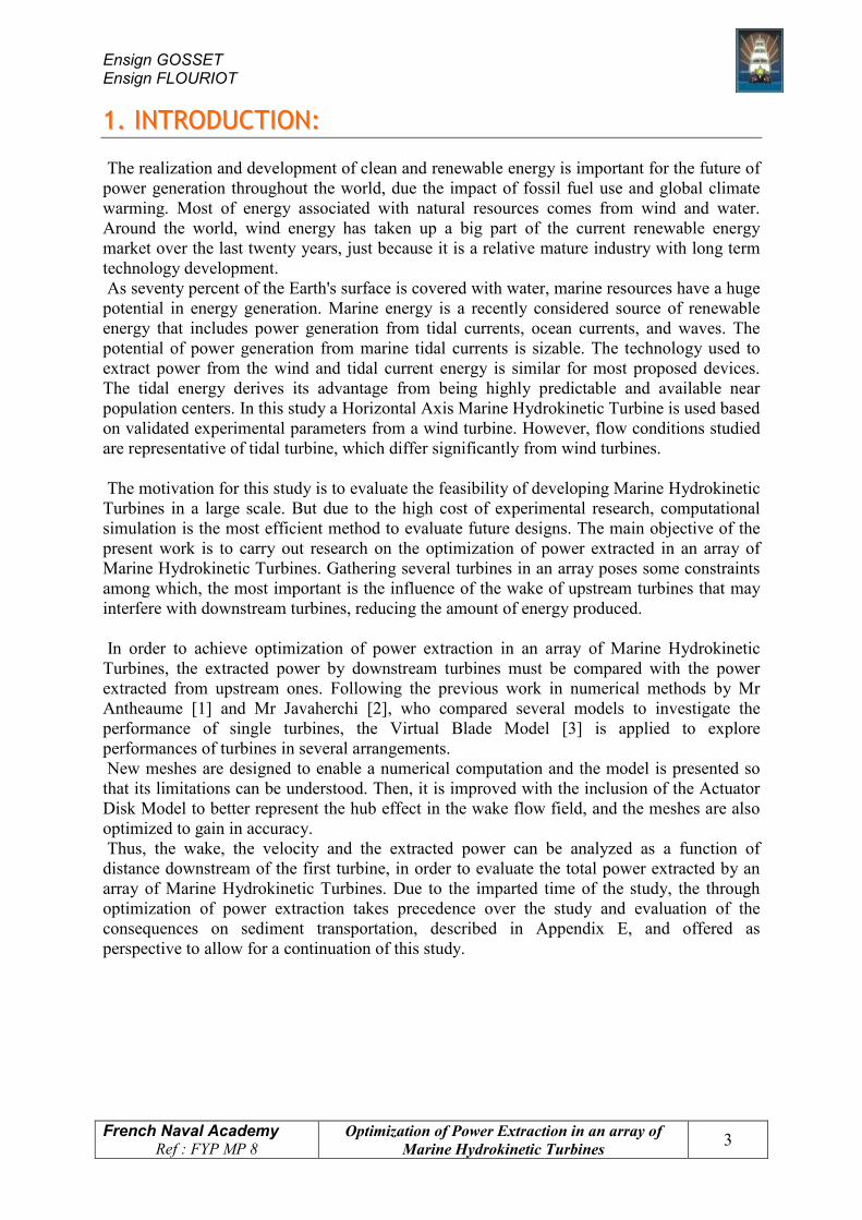
44.. IIMMPPRROOVVEEMMEENNTT OOFF TTHHEE MMOODDEELL With the VBM model we are able to model the turbine blades as a thin disk as it was explained in the previous Section 2.3, but VBM is not an adequate model to represent the hub since the lift would be zero at each section, but the drag would be very relevant. If the hub is not represented in the model due to its complexity, the flow passes through the hub area accelerating in a non-physical way. As a consequence the velocity increases in this area as does the power extracted. The velocity contour is represented below in Figure n° 14. This is not representative of what happens physically in reality. The velocity profile is continuous. In order to model the hub, we use the Actuator Disk Model explained in the following Section 4.1.

4.1 The Actuator Disk Model (ADM)

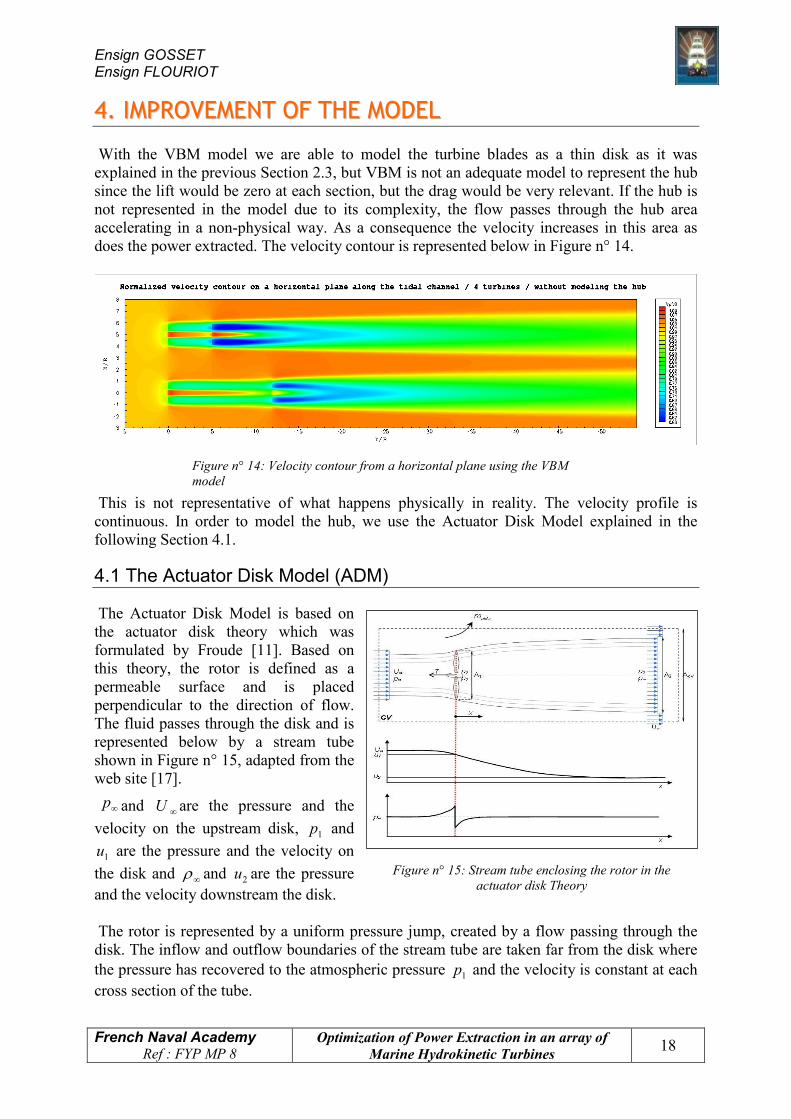
The Actuator Disk Model is based on the actuator disk theory which was formulated by Froude [11]. Based on this theory, the rotor is defined as a permeable surface and is placed perpendicular to the direction of flow. The fluid passes through the disk and is represented below by a stream tube shown in Figure n° 15, adapted from the web site [17].

∞p and ∞U are the pressure and the velocity on the upstream disk, 1p and

1u are the pressure and the velocity on the disk and ∞ρ and 2u are the pressure and the velocity downstream the disk. The rotor is represented by a uniform pressure jump, created by a flow passing through the disk. The inflow and outflow boundaries of the stream tube are taken far from the disk where the pressure has recovered to the atmospheric pressure 1p and the velocity is constant at each cross section of the tube.

Figure n° 14: Velocity contour from a horizontal plane using the VBM model

Figure n° 15: Stream tube enclosing the rotor in the actuator disk Theory




211

2

21

21

upUp ρρ +=+ ∞∞

22

211 2

121

upupp ρρ +=+∆− ∞

)(21 2

22 uUp −=∆ ∞ρ

22

1

uUu

+= ∞

∞

∞ −=U

uUa 1

aUu

212 −=∞

13

21

AUptotal ∞= ρ

11 uFPe =

11 ApF ∆=

11 uApPe ∆=

Applying Bernoulli equation, where ρ is the fluid density, upstream of the disk: (21) Applying Bernoulli equation downstream of the disk: (22) where p∆ is the pressure difference between the front and the back of the disk. Finally from equations (21) and (22), the pressure difference can be expressed as follow: (23) According to the theory by Froude [11], the velocity in the actuator disk is the average value of free stream and the far wake velocities: (24) The velocity at the actuator disk is lesser than the free stream velocity. The axial induction factor defined as follow represents the ratio of this reduction. (25) From equations (24) and (25), the relation between the velocities at each cross section of the tube will be as follow: (26) (27) The total power available in the flow can be written as: (28) where 1A is the surface of the disk. The power extracted by the actuator disk can be written as: (29) where 1F is the force of the flow on the disk and 1u is the velocity on the disk. The force of the flow on the disk can be expressed by: (30) From equations (29) and (30) the power extracted by the actuator disk can be rewritten as: (31)

aUu

−=∞

11




112

22 )(

21

uAuUPe −= ∞ρ

total

e

PP

=η

2)1(4 aa −=η

31

≤a

)21

( 22 νρν

αµ

CS +−=

21

3 )1(421

aaAUPe −= ∞ρ

mSp ∆−=∆

From the equation (23), the power extracted by the actuator disk is: (32) Finally, from equations (26) and (27), the power extracted by the actuator disk is: (33) The efficiency is defined by: (34) From equations (33) and (28) the efficiency can be written as: (35) Although not applicable to Marine Hydrokinetic turbines because of the interplay between potential energy and kinetic energy, the Betz limit [4] states that the maximum power coefficient is: (36) where maxeP is the maximum power extracted by the actuator disk. Therefore from equations (35) and (36), the axial induction factor is defined by the Betz limit by: (37) Instead of modelling the whole rotor in this theory we will only model the hub using ADM. The hub is then modelled as an actuator disk by using a porous media model in Fluent®. This porous media model is an added momentum sink, in the governing momentum equations. The porous media is modelled as an addition of a momentum source term to the standard fluid flow equation (18). This momentum sink contributes to the pressure drop that is proportional to the fluid velocity in the cell. The equation of this momentum sink in the case of simple homogeneous porous media is: (38) where S is the source term , ρ is the fluid viscosity,α is the face permeability of the media,

2C is the pressure jump coefficient and υ is the velocity normal to the porous face. This equation, which is representing the source term, is composed of two parts: a viscous loss term and an inertial loss term. As we know, this model can produce the desirable pressure drop defined in the following equation (39) due to the kinetic energy change of water across the disk. (39) where m∆ is the thickness of the media.

593.02716max ====

totale

ep P

PC η




mCp ∆+=∆ )21

( 22 νρν

αµ

Finally the pressure jump can be rewritten as: (40)

The viscous resistance coefficient α1

and the inertial resistance coefficient 2C are unknown

and will be setting in Fluent®. These coefficients were determined in the manner described as following: First, the value of the velocity on the disk is assumed to take a value close to the velocity at the beginning of the blades. This velocity was extracted from the post-processing with the software TecPlot®. Then, the value of the axial induction factor was determined from equation (26) where ∞U is the velocity at the inlet. In the first case of study, the inlet velocity

is constant and ∞U is equal to 1.2 −sm . From the value of the axial induction factor the efficiency can be determined from the equation (35). Then the velocities at each cross section of the tube and the pressure drop can be written in a table. In table n°3 represented below, the inlet velocity ∞U increases from 0 up to 1.4 −sm . The different velocities on the disk, and downstream the disk, are determined from equations (26) and (27). The pressure drop p∆ is determined from equation (23).

Table n° 3: Velocities for each cross section of the tube and pressure drop

From this table the pressure drop versus the velocity at the disk can be plotted. This plot is represented in Figure n°16, below.

∞U )1(1 aUu −= ∞ )21(2 aUu −= ∞ )(21 2

22 uUp −=∆ ∞ρ

].[ 1−sm ].[ 1−sm ].[ 1−sm ][Pa 0,0 0,000 0,000 0,000 … … … … 2,0 1,830 1,660 621,080 … … … … 4,0 3,660 3,320 2484,320

Figure n° 16: Pressure drop versus the velocity at the disk with an efficiency of 28:5%

u1 [m.s-1]

∆p [Pa]

1R

12x2Ex185.46y2

2

=

−+=

Pressure drop versus velocity

Poly. (Pressure drop versus velocity)




21211 uKuKp +=∆

mK∆

=µα

11m

KC

∆=ρ

22

2

From Figure n°16, a trend line is created through these points, yielding the following equation:

(41)

Finally the viscous resistance coefficient α1

and the inertial resistance coefficient 2C are

defined by: (42) (43) A hypothesis is made to determine the value of the velocity on the disk. 1.8.1 −sm is the first value chosen in accordance with the previous post processing, without any hub model. Using an iterative process, the best value of the velocity on the disk is determined by post processing the normalized velocity profile by the free stream velocity V0, downstream the first turbine as it is shown in Figure n° 17, below.

Figure n° 17: Velocity profile downstream the first turbine for different values of the velocity on the hub from 1.8 to 1.9 m.s-1




The best value for the velocity at the disk is 1.83.1 −sm . As a consequence, the efficiency is 28.5% .This translates into a power extracted by the hub equal to 7.2 kW. Since the hub does not contribute to the power extraction in reality, this power models the energy dissipation in the separated flow in the near wake of the hub. Based on the results shown on that previous Figure n°17, we determined that this ratio provided the most realistic velocity profile in the wake a few diameters downstream, which is the requirement to study the performance of the downstream turbines. In Fluent®, a cell zone is defined at the location of the hub in which the porous media model is applied. The pressure loss in the flow is determined via the user's input parameters which are given below as vector coordinates in the respective x, y, and z axis of the repair:

• Vector for the direction 1: x = 1, y = 0, z = 0 • Vector for the direction 2: x = 0, y = -1, z = 0, which is the direction of the flow. • The third direction is automatically defined as the normal to the two others directions.

Then the viscous resistance coefficient is setting at 1.66.10-08 2−m and the inertial resistance coefficient is setting at 11.3 −m in the three directions defined before. This establishment of a model for the hub is valid for a constant velocity at the inlet but also with a non linear velocity at the inlet because the velocity can be considered as uniform in the area of the hub. Indeed, the diameter of the hub is 2.844 meters. The velocity does not change significantly at the height of the hub. From equation (9) determined in Subsection 3.3.2, the velocity varies from 1.98.1 −sm to 1.02.2 −sm across the hub.

4.2 Analysis of the meshing sensitivity Now that the model is closer to reality in the wake of the rotor, another study is conducted to evaluate the direct impact of the mesh on simulation. As it is illustrated by Figures n°14 and n°17 the free stream velocity increases after passing the area of the rotor. It might be caused by the vicinity of the walls that accelerate the flow. To validate this observation and evaluate the impact on the accuracy of the measurement of power extracted, the next Subsections 4.2.1 to 4.2.3 describe the simulations in which the ADM is applied on the rotor. 4.2.1 Influence of the mesh refinement Two domains, with the same geometrical characteristics are compared to evaluate the impact of refining the meshing along the edges in the y direction, so the length lines that follow the orientation of the flow. Every boundary is at 3R from the center and the whole domain counts 385 088 nodes and 392 962 elements. The resolution at the inlet and the outlet are the same so the size of intervals before activating the ratio, is 1 meter for a 350 meters long domain. Refining the mesh consists in increasing the resolution of the mesh in a special area, but not in decreasing the whole resolution of the volume. In that way, activating a ratio launch an algorithmic calculation that makes the nodes closer and closer to each other in a defined direction.




Few ratio algorithms are available in Gambit® so that the ratio can be applied in: • The end of a edge by using the successive ratio as in Figure n°18 (a) • The middle of the edge by using the bell ratio as in Figure n°18 (b) • Two areas by using the inverted bell ratio as in Figure n°18 (c)

One advantage is that the total number of nodes and elements is conserved so that the time needed for the calculations should be close to each other with or without refinement. Another one is that the accuracy of measure will be better in the area where the intervals between the nodes are tightened. The disadvantage is the deterioration of accuracy in other areas. In this study it is interesting to evaluate this impact because as the accuracy in measuring speed is better by applying a ratio near the turbine, the extracted power measure will be more accurate too. The only constraint to ensure is to avoid any potential jump in discretization in the area of the rotor, by taking in account that in this zone, intervals between the nodes upstream and downstream must be as close as possible to each other as shown in Figure n°18 (a), where a successive refinements are applied on y-direction edges to reduce the resolution near the rotor. Upstream, the value of the ratio is 0.935 and it rises to 0.99 downstream. A measure of the extracted power for each case is computed. The results, presented in next table n°4, show that by applying the spacing ratio, the extracted power is exceeding of 5.1% the measured power on a uniform mesh. As the measure is more accurate, and as the extracted power is higher, every domain used to conduct the simulations in next subsections 4.2.2 and 4.2.3, is meshed with a spacing ratio. 4.2.2 Mesh resolution between inlet and turbine Another parameter to study is the resolution at the inlet. As the fluid flows along all the horizontal planes without any obstacle before the turbine, the velocity applied at the inlet is constant for each plane of the domain. So another factor that could impact the measures of velocity in the upstream area of turbines could be the resolution of the mesh along the y-axis. To conduct this calculation, the same domain is used, as in Subsection 4.2.1, applying different ratios at the inlet at the outlet. The goal of this study is to compare the extracted power of the two turbines. So from equation (44) below, two resolutions G are evaluated. The first one counts 25 intervals at the inlet and the second one 50 intervals in the same area, which means that the resolutions are respectively 0.5 and 1

(44)

Table n° 4: Extracted power and consequences due to the ratio

Impact on the mesh Power (W)

Without ratio Regular interval lengths 102954.94

With ratio Variable interval length 108487.18

mesh

i

lNb

G =

Figure n° 18: Different sorts of spacing ratios applied to y-axis edges

(a) Successive ratio on y-axis edges

Rotor area Equal interval lengths

(c) Inverted bell ratio on y-axis edges (b) Bell ratio on y-axis edges




where iNb is the number of interval counts and meshl is the length of the edge to mesh. For each mesh used to compute a solution, the ratio at the inlet is adapted to the resolution to avoid any jump of discretization. Moreover, three quadratic lines are created parallel to the y axis, with three different radial distances r to this axis. Then, solutions are computed to measure the extracted power for resolution at the inlet. The results are presented in following table n°5 and the differences of velocity measured along the quadratic lines in function of the mesh that is chosen are represented below, in Figure n°19 for four domains meshed with different number of grid points at the inlet and at the outlet, and with or without uniform spacing.

Resolution at the inlet

Total number of nodes in the mesh

Time of calculation using 4 cores Impact on the mesh Power (W)

G = 0.5 357 738 60 minutes Regular interval lengths 107 861,62

G = 1 385 088 67 minutes Variable interval length 108 487,18

.

Table n° 5: Impacts of resolution on the mesh, the computation time and the extracted power

Figure n° 19: Velocity versus normalized distance along three different longitudinal measuring lines

Inlet 50 / Outlet 300 with ratio

1,46

1,56

1,66

1,76

1,86

1,96

2,06

-15-10-50510Y/R [Radius]

Inlet 50 / Outlet 300 with ratio Inlet 50 / Outlet 300

1,46

1,56

1,66

1,76

1,86

1,96

2,06

-15-10-50510

Velocity [m/s]

Inlet 50 / Outlet 300

Y/R [Radius]


1,46

1,56

1,66

1,76

1,86

1,96

2,06

-15-10-50510Y/R [Radius]


Y/R [Radius]


1,46

1,56

1,66

1,76

1,86

1,96

2,06

-15-10-50510

Velocity [m/s]


Distance to the axis r = 1.2 m

Distance to the axis r = 4 m

Distance to the axis r = 3R

Inflexion point

Inflexion point




Table n°5 proves that the extracted power from the mesh with the better resolution is only exceeding of 0.5% the measured power of the other one, in which the resolution is half. Moreover the time of calculation is exceeding of 8.6% with the global resolution because of the rise in number of elements and nodes in the mesh. Once more it is also proved that the spacing ratio improves the results in the area of the rotor. Inflexion points can be seen at r = 4m for meshes without ratio. This highlights the lack of smooth evolution of the fluid variables as they go through the turbine disk when using these kinds of meshes. So, by analyzing these previous results, the best compromise to follow the study is to use a resolution of 0.5 at the inlet and a spacing ratio, to improve accuracy of measures near the rotor zone. In the next Subsection 4.2.3 the influence that the walls may have on the flow in the channel may be checked, without affecting too much the measure of power while keeping the most efficient accuracy and continuity near the rotor zone. 4.2.3 Influence of the domain width to turbine swept area As explained in Subsection 3.4.1 and proved by the analysis of Figures n°14 and n°17 the presence of the walls affects the measure of velocity. The last step of this analysis of meshing sensitivity consists in quantifying this impact to evaluate its importance, in order to choose the best dimensions for the future domains to simulate the flow in tidal channels and turbines realistically. In each of the previous simulations, it is evident, as in Figure n°19 that the velocity near the walls reaches its maximum three radiuses downstream of the turbines. So another series of calculation are conducted to measure the velocity in this area across all the width of the channel at z = 0, with a constant velocity at the inlet, by making the size of the channel, rW .2= , widen up from 4R to 22R. In this experiment, as the velocity at the inlet is constant, there is no variation of velocity in the inlet area on the z-axis, so the meshes are designed by scaling the front square shaped cross section of the previous mesh, and extruding it along the y axis. So the domain is as high as it is wide. Then the velocity versus the radial normalized distance to the axis X/R is plotted below in Figure n°20, three radiuses downstream of the turbine, to compare the effects of the walls in function of the distance from the axis of the turbine, which varies from 2R to 11 R. Figure n° 20: Normalized velocity versus radial distance from the axis three radiuses downstream of the turbine.

-2

-1

0

1

2

0,72 0,76 0,8 0,84 0,88 0,92 0,96 1 1,04Vy/V0

X/R

W = 22R W = 12R

W = 10R W = 8R

W = 6R W = 4R




This comparison of six curves, in relation with the width of the domain, proves that the free stream velocity increases when the domain is tightened. Then, it is decreasing with the distance from the walls. This decrease 10 −= VVyε , between the normalized velocity on the wall Vy/V0, that is measured and V0/V0 = 1 can be quantified in function of the distance Rrd tips −= , of the wall from the blade tips of the turbine. The distance tipsd is

chosen because tipsd = 0 is the minimal value of where a wall could be positioned. Using the previous measures from page 27, and given in table n°6 for the velocity three radiuses behind the turbine and one radius aside, a trend line is extrapolated in Excel®. This allows determining a law for this variation of velocity in function of tipsd , and therefore optimizing this distance with an acceptable size of mesh and time of computation. This plot is presented below in Figure n°21. In order to gain in accuracy, a retrospective of one unit is made to extrapolate the curve close to the origin, from the points given in table n°6, above. The deficit ε follows a -96/100 decreasing power-law as the distance of the wall from the tips increases. The decay rate velocity Ε , for a point of abscise tipsd is given by:

963.104256.0 −−==Ε tipstips

ddddε

and its variation is given by .0836.0 96322

2

2.-

tipstipstips

ddd

ddd

d==

Ε ε

The second derivative of the decrease ε is a decreasing power function so the variation of the decay rate Ε is less and less reduced as long as the domain is widened. It approaches 0.01 when the normalized distance exceeds 2 radiuses As a consequence we can agree that a good spacing between the tips of a turbine and the walls is included in the interval of 2 and 3 radiuses. This avoids manipulating too wide meshes and simplifies the design, while keeping coherent result, and an acceptable time of numerical computation.

W [R] r [R] dtips [R] Vy/V0 at (R, 3R, 0) ε = Vy/V0-1 4R 2 1 1,051645 0,05164 6R 3 2 1,02381 0,02381 8R 4 3 1,01401 0,01401 10R 5 4 1,00948 0,00947 12R 6 5 1,00772 0,00772 22R 11 10 1,00644 0,00643

Table n° 6: Variation of velocity three radiuses long and 1 radius aside downstream of the turbine.

Figure n° 21: Difference ε between Vy/V0 on the wall versus the radial distance from the tips.

0,00000

0,02000

0,04000

0,06000

0,08000

0,10000

0,12000

0,14000

0,16000

0,18000

0,20000

0 2 4 6 8 10Distance [Radius]]

Epsilon

Epsilon

Power (ε)

ε

9356.0

0442.02

963.0

=

= −

R

d tipsε

ε

dtips [Radius]

Ε ε




55.. RREESSUULLTTSS 5.1 Array of three turbines At first, we studied a case with three turbines in order to see the effects on the power, and the efficiency of the third turbine. Turbine n°3 is placed downstream, in the axis of Turbines n°1. Its distance varies from five to fifty radiuses, from the first ones, that are considered as the reference to measure the distances. The positions of the turbines in the domain are represented in Figure n° 22, based on the geometry presented in Subsection 3.1.2. 5.1.1Velocity contour and velocity profile The two goals of this part are to analyze the axisymmetric wake and the evolution of the velocity downstream of the first turbine, by using the VBM and ADM. First, the velocity contour is studied. Figure n° 23 represents the normalized velocity contour on a horizontal plane (x, y, z = 0), with an array of three turbines, where Turbine n°3 was positioned 50R downstream, coaxial with Turbine n°1. Close to the turbine, upstream and downstream the velocity decreases. Then the velocity recovers as the distance goes up. The centerline velocity, which is represented in Figure n°24, shows the velocity recovery.

Figure n° 23: Normalized velocity contour on a horizontal plane with a constant velocity at the inlet

Figure n° 22: Domain with three turbines

Turbine n° 3 at different positions (see top view in figure

n°35 (a) p38) Turbine n° 1

Turbine n° 2




The centerline velocity varies as 101

x . Then, the velocity profile is studied. The velocity contour and the velocity profile on a vertical plane (x = 0, y, z), the x position situated at the center of the turbine, are represented in Figure n°25. This plot allows analyzing the axis velocity profile.

(a) Constant velocity at the inlet

(b) Non linear velocity at the inlet

Figure n° 25: Normalized velocity contour and velocity profile on a vertical plane

Normalized centerline velocity

Power (Normalized centerline velocity)

0.9982R

0.6237xy2

0.1033

=

=Normalized centerline velocity [m.s-1]

Figure n° 24: Normalized centerline velocity versus distances

Distances (Radius)




yd VUV −= ∞

With a constant velocity at the inlet, the wake is axisymmetric. The velocity profile shows that moving further downstream turbine, the velocity deficit decreases. Downstream of the first line of turbines, the velocity deficit gets to its minimum value, at about 35R downstream. There is higher velocity deficit downstream the second turbine in comparison with the first turbine. This is due to the cumulative effect on the flow, as the wake of the upstream turbines is the inlet flow for Turbine n°3. Therefore at 35R downstream of Turbine n°3, the velocity deficit is larger than the corresponding velocity deficit downstream of the first turbine. At the top and bottom of each velocity profile a small acceleration is observed. The cause is the reduction of cross-sectional area. With a nonlinear velocity at the inlet, the velocity is not uniform, thus the wake is not axisymmetric. At the top, the velocity at the inlet is higher than the centerline velocity by 8.5%. As it is detailed in Subsection 3.2.2, at the top the velocity is equal to 2.2 m.s-1 instead of being 2 m.s-1, which was the value used with constant velocity at the inlet. Thus the acceleration of the flow at the top section is larger than with a uniform velocity. The same thing is observed at the bottom, where the deceleration of the flow is larger. In order to study the evolution of the velocity versus distances, the velocity profile at several distances downstream from 5R to 40R is plotted in Figure n°26. The distances chosen to trace that plot are according to a potential placement of Turbine n°3. As the distance increases, the velocity recovers to the free stream value. To confirm that this behavior closely matches the well-known decay of an axisymmetric wake in a turbulent flow, the velocity and momentum deficit are studied as in the next Subsection 5.1.2. 5.1.2 Velocity deficit and momentum deficit The velocity deficit is defined by the following equation:

(45)

dV is the centerline velocity deficit, ∞U is the uniform velocity at the inlet and yV is the centerline velocity in the y axis. According to canonical self similarity theory for the turbulent axisymmetric wake [12,

Subsection 5.4.4, p 151], for example, the centerline velocity deficit varies as 32

−x . In order to

validate the results from the simulations, the centerline velocity deficit is calculated for

Figure n° 26: Normalized velocity profile downstream turbine at the distance 5R, 8R, 10R, 12R, 15R, 20R, 25R, 30R, 40R with a constant velocity at the inlet

Vy/V0

Z/R




several distances downstream of the first turbine. Right after the turbine blade, the wake is inhomogeneous, but moving further downstream, it becomes axisymmetric. Due to the non homogeneity of the flow right after the device, the wake can not be considered as axisymmetric. Therefore the previously derived theory for decay of velocity deficit can not be applied in this region. As a result the velocity deficit is calculated from 10R to 50R downstream of the turbine and is represented versus distances in Figure n°27, below.

The centerline velocity deficit varies as 32

−x as it was expected and also as defined in

reference [12]. The same self-similarity theory [12] defines the momentum flow rate of the average flow from 0 to 3R as following: (46) where r is the radius, ρ the fluid density and ∞U is the velocity at the inlet. The momentum deficit is defined by the following equation:

(47) where dM& is the momentum deficit, ∞M& is the momentum at the inlet, which is defined

below and yM& is the momentum in the y axis. From equation (46), as the velocity at the inlet is uniform, the momentum at the inlet is defined by the following equation: (48)

∫ ∞=R

y drUrM3

0

22 ρπ&

yd MMM &&& −= ∞

29 ∞∞ = URM ρπ&

Centerline velocity deficit [m.s-1]

0.985R

2.096xy2

-0.665

=

=

Centerline velocity deficit

Power (Centerline velocity deficit)

Distance (Radius)

Figure n° 27: Centerline velocity deficit versus distances




3

21

VSCP pρ=

3

21

VS

PC p

ρη ==

The momentum yM& for each distance downstream of the first turbine and the momentum deficit are calculated from the results of the simulation, using the software package MatLab®. The original script is available in Appendix D. Finally the momentum deficit versus distance is represented in Figure n°28, below. For the same postulate as the velocity deficit, the momentum deficit can be calculated from 10R, the distance in which the wake becomes axisymmetric. The deficit should be constant, since it represents the reaction to the drag force exerted by the turbine on the flow. The results from the different cross sections in the simulation vary as

07.0x which is close to 0x . This good agreement with the theory supports the credibility of the simulations. The small increase in the momentum deficit is associated to the limited range over which we can integrate in the radial direction (up to 3R); for larger distances downstream, the wake occupies more of that range and there is a small loss in the integral that would be recovered if the integral could be extended to larger values of r. After having analyzed the flow downstream, the wake effect allows us to analyze both power and efficiency. 5.1.3 Power and efficiency The power is defined by the following equation:

(49)

P is the power, ρ is the fluid density, pC is the power coefficient, S is the surface of the

turbine and V is the velocity. From this equation (49) the efficiency η is defined by:

(50)

Momentum deficit [kg.m.s-1]

9724.0

508382

0707.0

=

=

R

xy

Momentum deficit versus distance Power (Momentum deficit versus distance) Distance (Radius)

Figure n° 28: Momentum deficit versus distance




61

45029 dP =

For the first two turbines the experimental power is equal to 95.2 kW with the efficiency of 24.83%. Then to study the effect of the distance of the third turbine, the power and the efficiency are plotted as a function of the distance where the third turbine is placed as it is shown in Figure n°29, below. The farther the third turbine is from the first ones, the more the power increases. The power increases because the velocity downstream in the wake that impinges on the downstream turbine increases with increased distance. The velocity contour is represented page 29 in Figure n° 23.

The power and therefore the efficiency are increasing as 61

x and the equation that describes this trend line is:

(51)

where P is the power and d the distance normalized by the radius between two turbine in the axial flow. In order to recover the initial extracted power from the first turbine, the distance between two turbines in the axial flow should be 87R. Table n°7, next page 35 contains the distance from which a third turbine should be placed to recover X% of the initial extracted by the first turbines. At this distance, the power and the efficiency should be at the maximum. The first turbine seems to interfere with the other one that is positioned downstream. Wake effects can be a problem for efficiency since a turbine placed right downstream another one would have a reduced incoming velocity and thus would output less power. Ideally we would like to avoid the effect of the wake created by the turbine. But in reality, due to the limited space available, complying with environmental issues, it is necessary to place the turbines closer to each other. This is all the more true that we are dealing with marine current turbines where the available high current velocity sites are narrow and limited in space. However, the more the turbines are in an array, the more is the power extracted. And it is necessary to deal with the spacing between them in order to optimize the power that could be extracted with the available space. Some perspectives have been taken into consideration. For example, by placing two turbines

Figure n° 29: Power and efficiency versus distances

Distances (Radius)

Power (W)

0.9988R

x11.739y2

0.1676

=

=

Efficiency (%)

Power versus distances

0.9988R

x45029y2

0.1676

=

=

Efficiency (Efficiency versus distances)

Power (Power versus distances)

Distances (Radius)

Efficiency versus distances




with a lateral offset of one radius the power extracted increases due to the wake effect. This part of the study is explained in Subsection 5.3.1.

Percentage of initial power Distance d (Radius) 100% 87 95% 64 90% 46 85% 33 80% 23 75% 16 70% 10

Table n° 7: Distance in which the power recovers X% of the initial power

5.2 Array of four turbines First at all, an arrangement of four turbines is experimented. The two last turbines, Turbine n°3 and Turbine n°4 move differently from 5R to 50R. Five cases are studied and figured below in Table n°8:

Distance of Turbine n°3

from Turbine n°1

Distance of Turbine n°4

from Turbine n°2 12R 5R 15R 10R 20R 8R 40R 25R 50R 30R

Table n° 8: Studied cases in an array of four turbines

5.2.1 Velocity contour The following Figure n°30, represents the normalized velocity contour on a horizontal plane (x, y, z = 0), for an array of four turbines with five different positions for the two last turbines, which are given under the profiles. In these contours, the velocity, downstream of the two first turbines, increases when the distance at which the turbines are placed increases. The further from Turbines n°1 and n°2 that Turbines n°3 and n°4 are positioned, the higher the incoming velocity on n°3 and n°4 is. As a consequence the velocity deficit is lower downstream of these.




(b) 10R / 15R

(c) 8R / 20R

(d) 25R / 40R

(e) 30R / 50R

(a) 5R / 12R

Figure n° 30: Normalized velocity contour on a horizontal plane with a velocity profile at the inlet.




5.2.2 Power and efficiency The next plots in Figure n°31 represent the power versus distances. On the blue curve there is an inflexion point between 20R and 25R. The accelerated flow caused by the existence of Turbine n°4, which is in front of Turbine n°3 decreases the amount of velocity deficit in the wake of Turbine n°1, which is inflow of Turbine n°3. As a result the extracted power by Turbine n°3, which is placed in the five configurations at 12R, 15R, 20R, 40R, and 50R increases. The extracted power by Turbine n°3 without the presence of Turbine n°4 is represented by the red point at 12R, 15R, 20R, 40R, and 50R. In order to study the difference of extracted power by Turbine n°3 with the presence of Turbine n°4, the same study done in Subsection 5.1.3 is repeated by fixing three turbines instead of two, and changing the distance of Turbine n°3 right downstream in the axis of the first one. In this configuration, which is represented in Figure n°32, Turbine n°4 is fixed and placed at 8R from Turbine n°2 and the location of Turbine n°3 is changed from 12R to 50R downstream of Turbine n°1. The main goal of this study is to compare the power extracted with an array of three turbines with another one of four turbines, in the perspective of studying the combined wake and distance effect, this comparison is illustrated below in Figure n°33. Therefore it allows the optimization of an array of turbines.

Figure n° 33: Power and efficiency versus distances.

Power (W) Efficiency (%)

Distance (Radius) Distance (Radius)

y = 48124x 0.1575

R2 = 0.9985 y = 44909x 0.1684

R2 = 0.9975

y = 12.545x 0.1575

R2 = 0.9985 y = 11,707x 0.1684

R2 = 0.9975

Array of 4 turbines

Array of 3 turbines

Array of 4 turbines

Power (Array of 3 turbines)

Array of 3 turbines Power (Array of 4 turbines)



Figure n° 32: Domain with four turbines.

Turbine n° 4

Turbine n° 3 at different positions (see top view in Figure

n°34 (b)). Turbine n° 1

Turbine n° 2

Figure n° 31: Power versus distances.

Power vs Distance

Power [W]

Distance [Radius]

Extracted power without Turbine n°4

Inflexion point




These results are showing that the power and therefore the efficiency increase as 35.61

x instead

of increasing as 61

x with three turbines. The following Figure n°34 represents the configuration of both arrays with three and four turbines. In a four-turbine array shown in Figure n°34 (b), the power extracted by Turbine n°3 is higher than the corresponding extracted power from the same turbine in the three-turbine array represented in Figure n°34 (a), More investigations confirm that the accelerated flow caused by the existence of Turbine n°4 decreases the amount of velocity deficit in the wake of Turbine n°1, which is the inflow of Turbine n°3. The lower velocity deficit in configuration (b) compared with (a) leads to gain more available energy inflow, hence more extracted power by the same turbine.

5.3 Optimization of an array of turbines The previous study made in Section 5.1 and 5.2 on the effect of the wake downstream turbine leads to envisage several arrangements with MHK turbines in order to optimize the power extracted in an array. 5.3.1 Array of two turbines The goal of this section is to compare the extracted power from a turbine located coaxially downstream the first one as next page 39, in Figure n° 35 (a) with another case, in which the turbines are not coaxial anymore and have an offset of 1R from their center as in Figure n° 35 (b). These two turbines are both placed at 12R from the first one.

#2

Figure n° 34: Top view of arrays of turbines.

(b) Array of four turbines.

(a) Array of three turbines.

30R

15R

#3 #1 #2

8R 10R 12R 15R

50R

40R

25R

20R

12R

#4

#3

#1 5R

20R

25R

40R

50R

30R

8R

3R 3R




The domain, which is represented in Figure n°35, has a square prism shape, extruded from a cross sectional square that is 8R wide, so 44.24 meters long. The LHS and RHS boundaries which define the edges of the domain are at 3R from the tips of the blades. This distance is longer than the one used in the previous domain, presented in Figure n°6 in order to decrease the effect of the wall. Indeed the velocity increases because of the presence of the outer wall. In reality the velocity should be uniform and equal to 2 1. −sm but in the conducted numerical simulation, it appears that the normalized velocity is greater than 1 in some locations near the edge of the domain. The following Figures n°36 (a) and 36 (b), are showing the velocity contour for these two configurations (a) and (b).

Figure n° 35: Placements of two coaxial (a) or offset (b) turbines in the domain.

Figure n° 36 (a): Normalized velocity contour on a horizontal plane (z=0) for a coaxial placement of two turbines.

Figure n° 36 (b): Normalized velocity contour on a horizontal plane (z=0) for an offset placement of two turbines.




Figure n° 38: Top view of an array of five turbines.

First of all, the velocity downstream the first turbine is greater at the tip of the blades than at the center as proved in Figure n°37. In comparing respectively Figures n° 36 (a) and 36 (b), it is observed that by placing a second turbine (b) downstream with an offset of 1R, the velocity upstream this one is more than the velocity upstream if it would have been on the same axis than the first turbine. As a result, the power extracted by the offset turbine is more than the power extracted by a coaxial turbine (a). The following table n°9 contains the power extracted by the turbines, the efficiency and the lost power. From this table, the efficiency of Turbine n°2 (b) is better than for Turbine n°2 (a). The difference of efficiency is 5%, but the difference in recovered power is 20%. In the same way, Turbine n°2 (b) loses less power than 2 (a).

As a result, improving the placement of the turbines by including an offset between them is a way to optimize the power extracted in an array of turbines.

POWER (kW) EFFICIENCY (%) LOST POWER (%) Turbine n°1 101 26.33 Turbine n°2(a): coaxial 64 16.68 36.63 Turbine n°2(b): offset 82 21.38 18.81

Table n° 9: Power, efficiency and lost power for each turbine.

5.3.2 Generalization of an array of turbine Studying the wake downstream of a turbine, the power and efficiency versus distances leads to consider an array of turbines to optimize the extracted power. Moreover the study carried out in previous Subsection 5.3.1 in comparing the power extracted by the second devices as a function of their position, allows designing an array with several turbines. The following Figure n°38 represents an array of five turbines.

Figure n° 37: Normalized Velocity 2R downstream the first turbine.




ideal

totale

Pn

P

.=η

The position of the turbines was judiciously evaluated in order to extract more power. To understand how the turbines interact between them, several cases are studied by choosing to activate three turbines in the VBM panel, then four and finally all of them. The following table contains the power extracted by the turbine for each case.

Turbines callsigns 123 125 127 1235 1237 1257 12357

P1 (kW) 96 96 96 96 96 96 96 P2 (kW) 96 96 96 96 96 96 96 P3 (kW) 104 104 104 104 P5 (kW) 79 69 79 69 P7 (kW) 75 75 53 53

Table n° 10: Extracted Power by each turbine in the array.

First, the effect of the Turbines n°1 and n°2 on Turbine n°3 is studied. The power extracted by the Turbine n°3 is 4% more than the power extracted by only one turbine in an array which is equal to about 100kW. This configuration is more efficient than in an array with two turbines, in which the second one would be placed with an offset. According to Figure n°37, at the tips of the blades the velocity increases and reaches its maximum. Turbine n°3 is placed between Turbines n°1 and n°2 at 4R downstream. The accelerated flow downstream n°1 and n°2 increases the free stream velocity, which is inflow of Turbine n°3. Upstream Turbine n°3 the velocity is more than upstream only one turbine. As a result the power extracted by Turbine n°3 is more than 100kW.

Then several observations can be made to compare the power extracted in the different arrays and see the effects of turbines on each other, by studying how the flow is coming upstream. The more the turbines are upstream of the last turbine, the more the velocity decreases and therefore the extracted power from this one is lower. For Turbine n°5 the power decreases of 13% in presence of Turbine n°3 upstream of it. For Turbine n°7 the power decreases of 30% in presence of Turbine n°5. At the opposite, the power extracted by Turbine n°7 is exactly the same when here is the Turbine n°3. The spacing between these two ones is 16R and this distance is sufficient so that the flow can recover a value close to the velocity upstream Turbine n°7, without the presence of Turbine n°3. In the case of Turbines n°1, n°2, n°3 and n°5 constituting the array, the power of Turbine n°5 decreases in comparison with the power this one can extract without the presence of Turbine n°3. The cause is that they are distant of 8R and this distance is not enough for the velocity to reach the same velocity with or without Turbine n°3. Finally the total extracted power by these different arrays is compared with the total power that the same number of considered turbines in each studied arrays, knowing that one turbine can individually extract 100kW. The efficiency is consequently defined as following using equation (52): (52) where n is the number of turbines in the array.




The following Figure n°39 represents the efficiency for the different studied arrays.

The efficiency rises up from 81% to 98.6%. This leaves us postulating that Horizontal Marine Hydrokinetic turbines could be deployed in high current sites in the near future. 5.3.3 Perspectives It could be interesting to study the power extracted in function of the offset between two turbines as it was studied in previous Subsection 5.3.1 in varying the lateral distance. According to Figure n°37 the velocity reaches at its maximum of 2m.s-1 from 1.2R. From this distance the power extracted will be at its maximum. Once in fixing this optimized distance, the power extracted can be again examined in varying the longitudinal distance between these two turbines. Moreover, the arrangement of the Turbine n°1, n°2 and n°3 studied in Subsection 5.3.2 could be also optimized in studying in the same way the evolution of the power extracted in function of the lateral and longitudinal distances. The more performing array is the previous one. To envisage designing an array, this arrangement should be used in placing several arrays of three turbines in front of the flow. It can be also conceivable to place several turbines on two or more rings of turbines. 5.3.4 Limitations of the numerical model The advantage of the computational method is to evaluate future designs of array of turbine in having some information on the viability and technical feasibility of an installation of turbine on high current sites. Indeed, due to a high cost, experiments are difficult to carry through, in order to investigate the power extracted and therefore the production of electricity. However computational model have some limitations. The computational domain is not exactly as in reality. One undesirable aspect is the presence of the wall which leads to extract more power than in reality because the velocity is accelerating. In reality the velocity from 1R of the tips of the blades should be uniform and equal to the free stream velocity. In the Subsection 4.2.3 it was shown that in widening the domain the velocity is closer to the real velocity.

Figure n° 39: Efficiency for different arrays of turbines.




66.. CCOONNCCLLUUSSIIOONN Due to high costs and difficulties to locate a good place to experiment in real high current sites because of merchant navigation, computational method is preferred to approach optimization of power extraction for Marine Hydrokinetic Turbines. Few models are available to study arrays. Based on the work from the department of Mechanical Engineering of the University of Washington, Seattle (WA), the Virtual Blade Model, adapted from aeronautical research, is selected from three other models, previously studied in the department. It represents the best compromise in terms of resolution, time of calculation and accuracy and therefore enables the representation of a two bladed turbine. The inclusion of body forces in a thin disk of fluid simulates the rotation of the blades, inside meshed domains, which stand in for a fluid channel. Then the VBM is improved to better represent the effect of the hub by addition of the Actuator Disk Model, to correct the velocity profile at the center of the turbine to produce a decrease in speed of the flow near the centerline of the wake that was previously increased due to a lack of drag in the hub between the blades. Then the dimensions of the meshes are confirmed by analyzing the sensitivity of meshing for a constant velocity at the inlet. Once the model is efficient, several cases of arrays are evaluated, combining from two to five turbines, to find the best arrangement for power extraction. First at all coaxial turbines are tested to quantify how the longitudinal distance between them affects the extracted power on the downstream one. It is demonstrated that the downstream turbine must be positioned eighty seven radiuses behind the front one to recover all its efficiency. So another solution to optimize the spacing is computed, by designing offset turbines. The results show a 50% decrease in lost power, in comparison with coaxial turbines at the same distance, an additional simulation is done consisting in placing a turbine downstream of two others. The aim is to reach the maximum extracted power as possible from the combined increase in speed aside the wakes generated by the front turbines. The analysis of power magnitude with simulations proves that models are in good agreement with our intuition, and some consequent progress is made in terms of optimization to gain in space, and efficiency in producing electricity with a clean, renewable energy. However the effects of turbulence in the wake can alter the transport of sediment in the tidal channels and this phenomenon needs to be studied. Actually, this is another important part of our study, concerning environmental impact that requires a different model to evaluate how turbulence is acting on the seabed, not to degrade it, to keep this type of clean energy viable. A few elements of this phenomenon are approached in Appendix E, to enable another team to continue this study, and give improve on these encouraging results by tracking particles. This would be a good complement to validate an affordable, efficient and clean source of power that must be completely safe for the marine environment. Moreover, in certain arrangements, as the velocity of the flow increases on downstream turbines, the magnitude of the forces applied on the blades and the shaft increases too. So other studies about cavitation at the tips or about material resistance of the blades should be conducted too. These are now the challenge for tomorrow.




AAppppeennddiixxeess

AAppppeennddiixx AA:: BBllaaddee cchhoorrdd aanndd ttwwiisstt ddiissttrriibbuuttiioonn

Section number Span Station (r/R) Chord Length (m) Twist angle (°)

1 0,25 0,7728 -18,074 2 0,273 0,711 -14,292 3 0,298 0,697 -11,909 4 0,353 0,666 -7,979 5 0,408 0,636 -5,308 6 0,424 0,627 -4,715 7 0,463 0,605 -3,425 8 0,518 0,574 -2,083 9 0,573 0,543 -1,15

10 0,576 0,542 -1,115 11 0,628 0,512 -0,494 12 0,683 0,482 0,015 13 0,727 0,457 0,381 14 0,739 0,451 0,475 15 0,794 0,42 0,92 16 0,849 0,389 1,352 17 0,864 0,381 1,469 18 0,904 0,358 1,775 19 0,959 0,328 2,191 20 1 0,305 2,5




AAppppeennddiixx BB:: LLiifftt aanndd ddrraagg ccooeeffffiicciieennttss vveerrssuuss tthhee aannggllee ooff aattttaacckk

lC dC

Reynolds number 750000.0 750000.0 Mach number 0.07 0.07

Number of data points 40 54

AOA (°) lC AOA (°) lC AOA (°) dC AOA (°) dC

-180.00 -0.5600 6.00 0.7521 -180.00 0.3027 8.00 0.0410 -172.00 -0.5600 8.00 0.9312 -175.00 0.3027 10.00 0.0512 -161.00 -0.5600 10.00 1.0854 -170.00 0.3027 12.00 0.0646 -147.00 -0.5600 12.00 1.2040 -165.00 0.3027 14.00 0.0838 -129.00 -0.5600 14.00 1.2578 -160.00 0.3027 16.00 0.1106 -49.00 -0.5600 16.00 1.2380 -140.00 0.3027 17.10 0.0994 -39.00 -0.5600 17.10 0.9400 -120.00 0.3027 18.10 0.2306 -20.10 -0.5600 18.10 0.8500 -110.00 0.3027 19.10 0.3142 -18.10 -0.6700 19.10 0.7000 -100.00 0.3027 20.10 0.3186 -16.10 -0.7900 20.10 0.6600 -90.00 0.3027 22.00 0.3694 -14.20 -0.8400 22.00 0.7000 -80.00 0.3027 24.10 0.4457 -12.20 -0.7000 24.10 0.7900 -70.00 0.3027 26.20 0.5260 -10.10 -0.6300 26.20 0.8800 -60.00 0.3027 30.00 0.5260 -8.20 -0.5600 39.00 0.8800 -50.00 0.3027 50.00 0.5260 -6.10 -0.6400 49.00 0.8800 -30.00 0.3027 60.00 0.5260 -4.10 -0.4200 129.00 0.8800 -20.10 0.3027 70.00 0.5260 -2.10 -0.2100 147.00 0.8800 -18.10 0.3069 80.00 0.5260 0.00 0.1344 161.00 0.8800 -16.10 0.1928 90.00 0.5260 2.00 0.3488 172.50 0.8800 -14.20 0.0898 100.00 0.5260 4.00 0.5564 180.00 0.8800 -12.20 0.0553 110.00 0.5260

40 data points -10.10 0.0390 120.00 0.5260 -8.20 0.0233 140.00 0.5260 -6.10 0.0112 160.00 0.5260 0.00 0.022725 165.00 0.5260 2.00 0.024253 170.00 0.5260 4.00 0.027739 175.00 0.5260 6.00 0.033265 180.00 0.5260 54 data points




AAppppeennddiixx CC:: IImmpplleemmeennttaattiioonn ooff tthhee UUDDFF #include "udf.h" # define Ui -2.0 /* Free stream velocity (m/s)*/ # define Zbottom -16.59 /* Depth (m)*/ DEFINE_PROFILE(inlet_velocity_new, thread, position) { real y[ND_ND]; /* this will hold the position vector */ real z; /* this identifies z as a variable */ face_t f; /*defines a face*/ begin_f_loop(f, thread) /*loop that steps through all faces in a thread*/ { F_CENTROID(y,f,thread);

/*returns coordinates of face centroid in array y[]*/ z = y[2]; F_PROFILE(f, thread, position)=Ui*pow(((z-Zbottom)/Zbottom),(1/7)); } end_f_loop(f, thread) }




clc; close all; clear all; n_data=4; % n_data is the number of data columns in the file exported from Tecplot file='40Raure_matlab_cut1_4R.txt'; fid=fopen(file,'r'); for j=1:n_data+16, %skipping definition lines in data text file fgetl(fid); end

%reading and loading variables X, Y,Z, Vy [data,count]=fscanf(fid,'%f',[n_data inf]); fclose(fid); l=length(data); X_x=data(1,:); X_y=data(2,:); X_z=data(3,:); V_y=data(4,:); %momentum at the inlet M_inf = 9 * pi * 5.53 * 5.53 * 998.2 * 2 * 2 % calculating the average velocity for each segment for j=1 : length(X_x)-1 V_ave(j,1) = (0.5 * (V_y(j)+V_y(j+1)) ); end % finding the area of that segment for j=1 : length(X_x)-1 dA(j,1) = pi * ((X_z(j))^2 - (X_z(j+1))^2); end % calculating the momentum on each segment for j=1 : length(X_x)-1 M_y(j,1) = 998.2 * V_ave(j,1) * V_ave(j,1) * dA(j,1); end % Adding up the values of momentum deficit of different segments (integrating) M_total=sum(M_y) %Momentum deficit on the specific plane M_deficit = M_inf - M_total

AAppppeennddiixx DD:: MMaattLLaabb®® SSccrriipptt ffoorr ccaallccuullaattiioonn ooff tthhee mmoommeennttuumm ddeeffiicciitt




AAppppeennddiixx EE:: PPaarrttiicclleess ttrraacckkiinngg The goal of this study is to determine the impact of the presence of turbines on the sedimentation of the particle on seabed. To study this four different sizes of particles are injected at the inlet and Discrete Phase Model (DPM) and Discrete Random walk (DRW) models are used to predict the trajectories of these particles. DPM models the trajectories of particles based on the mean fluid phase velocity u . To predict the dispersion of the particles due to turbulence, the instantaneous value of the fluctuating gas flow velocity 'u , is included. As a result, the velocity is defined by: 'uuu += Using only the DPM can provide some information on the sedimentation of the particles on seabed. These results are showed in Figure n°40 where 400 particles are injected at the inlet on a plane which is a square with 7 meters long sides. Between 50 and 100 meters downstream turbine, the sedimentation of particles is increased by 2% of the total number particles due to the velocity deficit in the wake of the turbine. Then, the number of particles sedimenting decreases. At the center of the turbine the velocity is lower and this effect can be observed in the second plot. The presence of the turbine leads to have more sedimented particles on seabed from 50 meters downstream and then less sedimented particles from 200 meters. This can impact the geometry and the sedimentation on seabed. These results can give us an approximation of the effect of the sedimented particles on seabed but as this model is based only on the mean velocity, the sedimentation is not realistic. Adding DRW can better describe the trajectories of particles due to turbulence. In this model the fluctuating velocity components are discrete piecewise constant functions of time given by the characteristic lifetime of eddies. The obtained results are not those expected. Indeed the turbulence model used, SST k-ω model, which assumes isotropy, leads to high level of fluctuations perpendicular to the bottom wall and to an over-prediction of particle dispersion by the turbulence fluctuations. This model predicts particle trajectories where the particles move in and out of the wake and therefore are not subject to the wake effects except for a short fraction of their trajectories. The effect on sedimentation is then significantly under predicted. Further investigation by Teymour Javerherchi and Dr. Alberto Aliseda seem to indicate that using the Reynolds stress model instead of the SST k-ω model could provide a better prediction of the deposition rates of sediment particles. Indeed this model, which account for the anisotropy of turbulence, provides a more accurate description of the turbulent flow field near the bottom wall. Modeling the flow with this model would be a first step in improving the accuracy of the predictions from the computational simulations and studying the environmental effect on the seabed of Marine Hydrokinetic turbines.

Figure n°40: Percentage of Sedimented Particles on seabed without turbine (left) and with turbine (right).




AAppppeennddiixx FF:: GGaanntttt ddiiaaggrraamm

Aug

ust

Sept

embe

r N

ovem

ber

N

ovem

ber

Oct

ober

Pres

enta

tion

coac

hing

Tue

sday

, 16t

h N

ovem

ber

Frid

ay, 1

7th

Dec

embe

r

Pres

enta

tion

Mem

oir

layo

ut

Pres

enta

tion

at th

e M

echa

nica

l E

ngin

eeri

ng

Dep

artm

ent

in th

e U

nive

rsity

of

Was

hing

ton

Des

igni

ng

the

post

er

Mem

oir w

ritin

g

Lea

rnin

g

the

Softw

are:

Fl

uent

®,

Gam

bit®

T

ecpl

ot®

Mod

elin

g si

ngle

turb

ine

dom

ain

and

offs

et a

rray

s.

Firs

t pos

t pr

oces

sing

Dis

tanc

e w

ork

usin

g a

FTP

serv

er fr

om F

renc

h N

aval

A

cade

my

to e

xcha

nge

wor

k fil

es fo

r Flu

ent®

and

Gam

bit®

. W

ritin

g th

e m

emoi

r usi

ng th

e co

rrec

tion

func

tion

of th

e so

ftw

are

Wor

d®, a

nd

exch

angi

ng fi

les

regu

larl

y.

Exp

erim

ent a

bout

par

ticle

tr

acki

ng

Eva

luat

ion

abou

t mes

hing

se

nsiti

vity

Impr

ovem

ent o

f the

m

odel

. D

efin

ition

of

the

para

met

ers

for t

he

hub,

firs

t tes

t. D

esig

n of

the

mul

ti tu

rbin

e ar

ray.




RReeffeerreenncceess Classical references

[1] Sylvain Antheaume. Modeling a wind turbine, comparison of the SRF and VBM models. August 18, 2009.

[2] Amir Teymour Javaherchi. Numerical Modeling of Tidal Turbines: Methodology Development and Potential Physical Environmental Effects. Master thesis, November 2010.

[3] Michael Ruith Sutikno Wirogo. Virtual Blade Model. 2004.

[4] L.J. Fingersh D.W. Jager J.R. Cotrell S. Schreck M.M. Hand, D.A. Simms and S.M. Larwood. Unsteady aerodynamics experiment phase VI: Wind tunnel test configurations and available data campaigns. National Renewable Energy Laboratory (NREL) / TP-500-29955, December 2001.

[5] Xiaojing Sun. Numerical and experimental investigation of tidal current energy extraction. University of Edinburgh, 2008.

[6] Tutorial of the Virtual Blade Model.

[7] Bruce R. Munson, Donald F. Young, Theodore H. Okiishi, Fundamentals of fluid mechanics, 4th Edition.

[8] F. R. Menter. Two-Equation Eddy-Viscosity Turbulence Models for Engineering Applications. AIAA Journal, Vol. 32 No. 8 pp. 1598-1605, August 1994.

[9] Theory guide. Ansys Fluent® 12.0, April 2009.

[10] User’s guide. Ansys Fluent® 12.0, April 2009.

[11] R. E. Froude. On the played in propulsion by difference in pressure. Transaction of the Institute of Naval Architects, vol. 30, pp. 390-423, 1889.

[12] Stephen B. Pope. Turbulent flows. Cambridge University press, 2000.

Web references [13] National Oceanic and Atmospheric Administration: Tidal Current tables – Strait of

San Juan de Fuca, Predicted Tidal Currebt [On line]. 27th October, 2010 – [Updated on 2010-10-15]. TXT files. Available on the Internet: <http://www.co-ops.nos.noaa.gov/currents04/STAITJD.shtml>.

[14] National Oceanic and Atmospheric Administration: Office of Coast Survey – Strait of San Juan de Fuca to Strait of Georgia Nautical Chart n°18421. [On line]. 27th October, 2010 – [Updated on 2010/10/19]. Flash Player File. Software to read the file: Adobe flash player 9.0.

Available on the Internet: <http://www.co-ops.nos.noaa.gov/OnLineViewer/18421.shtml>.

http://www.co-ops.nos.noaa.gov/currents04/STAITJD.shtm

http://www.co-ops.nos.noaa.gov/OnLineViewer/18421.shtm




[15] Fluent®: User’s help - Modeling Turbulent Flows in Fluent®. [On line]. 4th November, 2010 – [Updated on 2010/10/30]. PDF Document. Software to read the file: Adobe Acrobat Reader.

<http://www.fluent.com/software/university/blog/turbulent.pdf>.

[16] University of Starthclyde: Energy Research Unit - Momentum Theory by Froude for an Actuator Disk [On line]. October 2010 – [Updated on 2010-10-18]. Available on the Internet: <http://www.esru.strath.ac.uk/EandE/Web_sites/05-06/marine_renewables/technology/Froude.htm>.

http://www.fluent.com/software/university/blog/turbulent.pdf

A Gosset G Flouriot Report - University of Washington

Documents

Transcript of A Gosset G Flouriot Report - University of Washington