A globally divergence-free discontinuous galerkinmethod for induction and related equations

Praveen Chandrashekarpraveen@math.tifrbng.res.in

Center for Applicable MathematicsTata Institute of Fundamental Research

Bangalore-560065, Indiahttp://cpraveen.github.io

GIAN Course on Computational Solution of Hyperbolic PDEIIT Delhi, 4–15 December 2017

Supported by Airbus Foundation Chair at TIFR-CAM, Bangalorehttp://math.tifrbng.res.in/airbus-chair

1 / 55

Joint work withDinshaw Balsara

Univ. of Notre Dame

2 / 55

Maxwell EquationsLinear hyperbolic system

∂B

∂t+∇×E = 0,

∂D

∂t−∇×H = −J

B = magnetic flux density D = electric flux densityE = electric field H = magnetic field

J = electric current density

B = µH, D = εE, J = σE µ, ε ∈ R3×3 symmetric

ε = permittivity tensor

µ = magnetic permeability tensor

σ = conductivity

∇ ·B = 0, ∇ ·D = ρ (electric charge density),∂ρ

∂t+∇ · J = 0

3 / 55

Ideal MHD equationsNonlinear hyperbolic system

Compressible Euler equations with Lorentz force

∂ρ

∂t+∇ · (ρv) = 0

∂ρv

∂t+∇ · (pI + ρv ⊗ v −B ⊗B) = 0

∂E

∂t+∇ · ((E + p)v + (v ·B)B) = 0

∂B

∂t−∇× (v ×B) = 0

Magnetic monopoles do not exist: =⇒ ∇ ·B = 0

4 / 55

Model problem

∂B

∂t+∇×E = −M

Divergence evolves according to

∂

∂t(divB) +∇ ·M = 0 (1)

In 2-D∂Bx

∂t+∂Ez

∂y= −Mx,

∂By

∂t− ∂Ez

∂x= −My

5 / 55

Model problem

In MHD, B represents the magnetic field and M = 0

∂B

∂t+∇×E = 0, E = −v ×B

Magnetic monopoles do not exist: =⇒ ∇ ·B = 0If

∇ ·B = 0 at t = 0

then

∂

∂t(∇ ·B) +∇ · ∇ ×E = 0 =⇒ ∇ ·B = 0 for t > 0

In 2-D, the induction equation can be written as

∂Bx

∂t+∂E

∂y= 0,

∂By

∂t− ∂E

∂x= 0, E = vyBx − vxBy

6 / 55

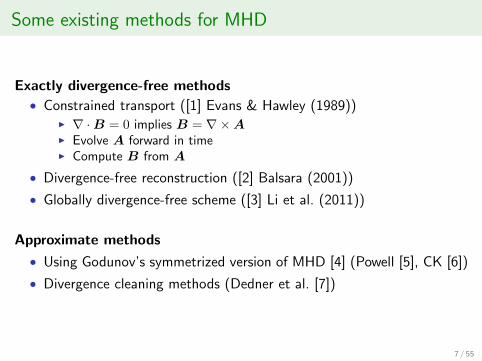
Some existing methods for MHD

Exactly divergence-free methods

• Constrained transport ([1] Evans & Hawley (1989))I ∇ ·B = 0 implies B = ∇×AI Evolve A forward in timeI Compute B from A

• Divergence-free reconstruction ([2] Balsara (2001))

• Globally divergence-free scheme ([3] Li et al. (2011))

Approximate methods

• Using Godunov’s symmetrized version of MHD [4] (Powell [5], CK [6])

• Divergence cleaning methods (Dedner et al. [7])

7 / 55

Approximation of magnetic field

When dealing with problems where the vector field B must bedivergence-free, it is natural to look for solutions in H(div,Ω) which isdefined as

H(div,Ω) = B ∈ L2(Ω) : div(B) ∈ L2(Ω)

To approximate functions in H(div,Ω) on a mesh Th, we need thefollowing compatibility condition.

Theorem (See [8], Proposition 3.2.2)

Let Bh : Ω→ Rd be such that

1 Bh|K ∈H1(K) for all K ∈ Th2 for each common face F = K1 ∩K2, K1,K2 ∈ Th, the trace of

normal component n ·Bh|K1 and n ·Bh|K2 is the same.

Then Bh ∈ H(div,Ω). Conversely, if Bh ∈ H(div,Ω) and (1) holds, then(2) is also satisfied.

8 / 55

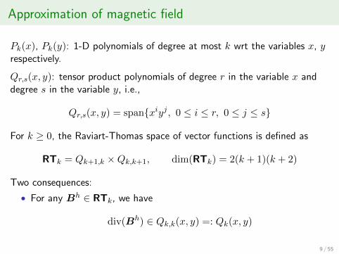
Approximation of magnetic field

Pk(x), Pk(y): 1-D polynomials of degree at most k wrt the variables x, yrespectively.

Qr,s(x, y): tensor product polynomials of degree r in the variable x anddegree s in the variable y, i.e.,

Qr,s(x, y) = spanxiyj , 0 ≤ i ≤ r, 0 ≤ j ≤ s

For k ≥ 0, the Raviart-Thomas space of vector functions is defined as

RTk = Qk+1,k ×Qk,k+1, dim(RTk) = 2(k + 1)(k + 2)

Two consequences:

• For any Bh ∈ RTk, we have

div(Bh) ∈ Qk,k(x, y) =: Qk(x, y)

9 / 55

Approximation of magnetic field

• The restriction of Bh = (Bhx , B

hy ) to a face is a polynomial of degree

k, i.e.,

Bhx(±∆x/2, y) ∈ Pk(y), Bh

y (x,±∆y/2) ∈ Pk(x)

For doing the numerical computations, it is useful to map each cell to areference cell.

ξi, 0 ≤ i ≤ k + 1 = Gauss-Lobatto-Legendre (GLL) nodes

ξi, 0 ≤ i ≤ k = Gauss-Legendre (GL) nodes

Let φi and φi be the corresponding 1-D Lagrange polynomials. Then themagnetic field is given by

Bhx(ξ, η) =

k+1∑i=0

k∑j=0

(Bx)ijφi(ξ)φj(η), Bhy (ξ, η) =

k∑i=0

k+1∑j=0

(By)ijφi(ξ)φj(η)

10 / 55

Approximation of magnetic field

Bx ∈ Q1,0 By ∈ Q0,1

Location of dofs of Raviart-Thomas polynomial for k = 0

Bx ∈ Q2,1 By ∈ Q1,2

Location of dofs of Raviart-Thomas polynomial for k = 1

11 / 55

Approximation of magnetic field

Bx ∈ Q3,2 By ∈ Q2,3

Location of dofs of Raviart-Thomas polynomial for k = 2

Our choice of nodes ensures that the normal component of the magneticfield is continuous on the cell faces.

We have the error estimates on Cartesian meshes [9], [10]

‖B −Bh‖L2(Ω) ≤ Chk+1|B|Hk+1(Ω)

‖div(B)− div(Bh)‖L2(Ω) ≤ Chk+1|div(B)|Hk+1(Ω)

12 / 55

Construction of Bh from moments

e+xe−x

e−y

e+y

C

0 1

2 3The edge moments are given by∫

e∓x

Bhxφdy ∀φ ∈ Pk(y)

and ∫e∓y

Bhyφdx ∀φ ∈ Pk(x)

The cell moments are given by∫CBh

xψdxdy ∀ψ ∈ ∂xQk(x, y) := Qk−1,k(x, y)

13 / 55

Construction of Bh from moments

and ∫CBh

yψdxdy ∀ψ ∈ ∂yQk(x, y) := Qk,k−1(x, y)

Note thatdimPk(x) = dimPk(y) = k + 1

anddim ∂xQk(x, y) = dim ∂yQk(x, y) = k(k + 1)

so that we have in total

4(k + 1) + 2k(k + 1) = 2(k + 1)(k + 2) = dim RTk

The moments on the edges e∓x uniquely determine the restriction of Bhx on

those edges, and similarly the moments on e∓y uniquely determine the

restriction of Bhy on the corresponding edges. This ensures continuity of

the normal component of Bh on all the edges.

14 / 55

Theorem

If all the moments are zero for any cell C, then Bh ≡ 0 inside that cell.

Proof: The edge moments being zero implies that

Bhx ≡ 0 on e∓x and Bh

y ≡ 0 on e∓y

Now take ψ = ∂xφ for some φ ∈ Qk in the cell moment equation of Bhx

and perform an integration by parts

−∫C

∂Bhx

∂xφdxdy −

∫e−x

Bhxφdy +

∫e+x

Bhxφdy = 0

and hence ∫C

∂Bhx

∂xφdxdy = 0 ∀φ ∈ Qk

Since ∂Bhx

∂x ∈ Qk, this implies that ∂Bhx

∂x ≡ 0 and hence Bhx ≡ 0. Similarly,

we conclude that Bhy ≡ 0.

15 / 55

Theorem

Let Bh ∈ RTk satisfy the moments∫e∓x

Bhxφdy =

∫e∓x

Bxφdy ∀φ ∈ Pk(y) (2)∫e∓y

Bhyφdx =

∫e∓y

Byφdx ∀φ ∈ Pk(x) (3)∫CBh

xψdxdy =

∫CBxψdxdy ∀ψ ∈ ∂xQk(x, y) (4)∫

CBh

yψdxdy =

∫CByψdxdy ∀ψ ∈ ∂yQk(x, y) (5)

for a given vector field B ∈ H(div,Ω). If div(B) ≡ 0 then div(Bh) ≡ 0.

16 / 55

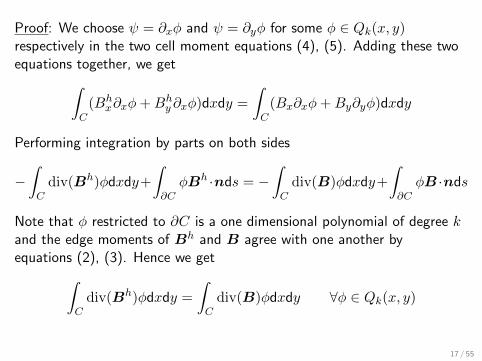
Proof: We choose ψ = ∂xφ and ψ = ∂yφ for some φ ∈ Qk(x, y)respectively in the two cell moment equations (4), (5). Adding these twoequations together, we get∫

C(Bh

x∂xφ+Bhy ∂xφ)dxdy =

∫C

(Bx∂xφ+By∂yφ)dxdy

Performing integration by parts on both sides

−∫C

div(Bh)φdxdy+

∫∂CφBh ·nds = −

∫C

div(B)φdxdy+

∫∂CφB ·nds

Note that φ restricted to ∂C is a one dimensional polynomial of degree kand the edge moments of Bh and B agree with one another byequations (2), (3). Hence we get∫

Cdiv(Bh)φdxdy =

∫C

div(B)φdxdy ∀φ ∈ Qk(x, y)

17 / 55

If div(B) ≡ 0 then∫C

div(Bh)φdxdy = 0 ∀φ ∈ Qk(x, y)

Since div(Bh) ∈ Qk(x, y) this implies that div(Bh) ≡ 0 everywhere insidethe cell C.

Remark: The proof makes use of integration by parts for which thequadrature must be exact. The integrals involving Bh can be evaluatedexactly using Gauss quadrature of sufficient accuracy. This is not the casefor the integrals involving B since it can be an arbitrary nonlinearfunction. When div(B) = 0, we have B = (∂yΦ,−∂xΦ) for some smoothfunction Φ. We can approximate Φ by Φh ∈ Qk+1 and compute theprojections using (∂yΦh,−∂xΦh) in which case the integrations can beperformed exactly.

18 / 55

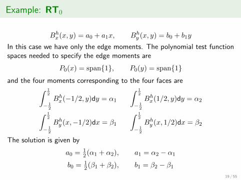
Example: RT0

Bhx(x, y) = a0 + a1x, Bh

y (x, y) = b0 + b1y

In this case we have only the edge moments. The polynomial test functionspaces needed to specify the edge moments are

P0(x) = span1, P0(y) = span1and the four moments corresponding to the four faces are∫ 1

2

− 12

Bhx(−1/2, y)dy = α1

∫ 12

− 12

Bhx(1/2, y)dy = α2∫ 1

2

− 12

Bhy (x,−1/2)dx = β1

∫ 12

− 12

Bhy (x, 1/2)dx = β2

The solution is given by

a0 = 12(α1 + α2), a1 = α2 − α1

b0 = 12(β1 + β2), b1 = β2 − β1

19 / 55

Example: RT1

Bhx(x, y) = a0 + a1x+ a2y + a3xy + a4(x2 − 1

12) + a5(x2 − 112)y

Bhy (x, y) = b0 + b1x+ b2y + b3xy + b4(y2 − 1

12) + b5x(y2 − 112)

The polynomial test function spaces needed to specify themoments (2)-(5) are

P1(x) = span1, x, P1(y) = span1, y

∂xQ1(x, y) = span1, y, ∂yQ1(x, y) = span1, x

20 / 55

Example: RT2

The polynomial test function spaces needed to specify the edge momentsare

P2(x) = span1, x, x2 − 112, P2(y) = span1, y, y2 − 1

12

while those needed for the cell moments are given by

∂xQ2(x, y) = span1, x, y, xy, y2 − 112 , x(y2 − 1

12)

∂yQ2(x, y) = span1, x, y, xy, x2 − 112 , (x

2 − 112)y

21 / 55

DG scheme for the induction equation

Constructing Bh from the edge and cell moments allowed us to getdivergence-free approximation.

We will construct a scheme to evolve the same moments in time.

e+xe−x

e−y

e+y

C

0 1

2 3 Consider the right edge e+x . Multiply by test

function φ ∈ Pk(y)∫e+x

(∂Bx

∂t+∂E

∂y

)φdy = −

∫e+x

Mxφdy

and integrate by parts in second term∫e+x

∂Bx

∂tφdy −

∫e+x

E∂φ

∂ydy + (Eφ)3 − (Eφ)1 = −

∫e+x

Mxφdy

22 / 55

DG scheme for the induction equation

Edge moments are evolved by∫e∓x

∂Bhx

∂tφdy −

∫e∓x

E∂φ

∂ydy + [Eφ]e∓x = −

∫e∓x

Mxφdy, ∀φ ∈ Pk(y)

∫e∓y

∂Bhy

∂tφdx+

∫e∓y

E∂φ

∂xdx− [Eφ]e∓y = −

∫e∓y

Myφdy, ∀φ ∈ Pk(x)

where

E = numerical flux from a 1-D Riemann solver required on the faces

E = numerical flux from a multi-D Riemann solver needed at vertices

[Eφ]e−x = (Eφ)2 − (Eφ)0, [Eφ]e+x

= (Eφ)3 − (Eφ)1

[Eφ]e−y = (Eφ)1 − (Eφ)0, [Eφ]e+y

= (Eφ)3 − (Eφ)2

23 / 55

DG scheme for the induction equation

The cells moments are evolved by the following standard DG scheme∫C

∂Bhx

∂tψdxdy −

∫C

E∂ψ

∂ydxdy +

∫∂C

Eψnyds = −∫C

Mxψdxdy, ∀ψ ∈ ∂xQk(x, y)

∫C

∂Bhy

∂tψdxdy +

∫C

E∂ψ

∂xdxdy −

∫∂C

Eψnxds = −∫C

Myψdxdy, ∀ψ ∈ ∂yQk(x, y)

Note that the same 1-D numerical flux E is used in both the edgeand cell moment equations whereas the vertex numerical flux E isneeded only in the edge moment equations.

24 / 55

Theorem

Assuming that M = 0, the DG scheme (22)-(22) preserves the divergenceof the magnetic field.

Proof: For any φ ∈ Qk(x, y) take ψ = ∂xφ and ψ = ∂yφ in the two cellmoment equations respectively and add them together to obtain∫

C

[∂Bh

x

∂t∂xφ+

∂Bhy

∂t∂yφ

]dxdy −

∫∂CE(nx∂yφ− ny∂xφ)ds = 0

Note that two of the cell integrals cancel since ∂x∂yφ = ∂y∂xφ.Performing an integration by parts in the first term, we obtain

−∫Cφ∂

∂tdiv(Bh)dxdy+

∫∂Cφ∂

∂t(Bh·n)ds−

∫∂CE(nx∂yφ−ny∂xφ)ds = 0

25 / 55

Now, let us concentrate on the last two terms which can be re-arranged asfollows ∫

e+x

φ∂Bh

x

∂tdy −

∫e−x

φ∂Bh

x

∂tdy +

∫e+y

φ∂Bh

y

∂tdx−

∫e−y

φ∂Bh

y

∂tdx

−∫e+x

E∂yφdy +

∫e−x

E∂yφdy +

∫e+y

E∂xφdx−∫e−y

E∂xφdx

The restriction of φ on each edge is a one dimensional polynomial ofdegree k. We can use the edge moment equations to simplify as

=− [Eφ]e+x

+ [Eφ]e−x

+ [Eφ]e+y− [Eφ]

e−y

=− (Eφ)3 + (Eφ)1 + (Eφ)2 − (Eφ)0 + (Eφ)3 − (Eφ)2 − (Eφ)1 + (Eφ)0

= 0

Hence we have∫Cφ∂

∂tdiv(Bh)dxdy = 0 ∀φ ∈ Qk(x, y)

Since div(Bh) ∈ Qk(x, y) we conclude that the divergence is preserved bythe numerical scheme.

26 / 55

Remark: The above proof required integration by parts in the termsinvolving the time derivative. These integrals can be computed exactlyusing Gauss quadrature of sufficient order. The other cell integral in theDG scheme can be computed using any quadrature rule of sufficient orderand need not be exact. All the edge integrals which involve the numericalflux E appearing in the edge moment and cell moment evolution equationsmust be computed with the same rule and it is not necessary to be exactfor the above proof to hold. However, from an accuracy point of view,these quadratures must be of a sufficiently high order to obtain optimalerror estimates.

Remark: The preservation of divergence does not rely on the specific formof the fluxes E, E but only on the fact that we have a unique flux E at allthe vertices, and that we use the same 1-D numerical flux E in both theedge and cell moment equations.

27 / 55

Theorem (M 6= 0)

The divergence evolves consistently with equation (1) in the sense that∫Cφ∂

∂tdiv(Bh)dxdy−

∫CM ·∇φdxdy+

∫∂CφM ·nds = 0, ∀φ ∈ Qk

Since div(Bh) ∈ Qk, we can expect div(Bh) to be accurate to O(hk+1).

In case of Maxwell equations, if we want to compute charge density

ρ = ∇ ·D

we can get ρ to same accuracy as the vector fields, even though we take aderivative !!!

28 / 55

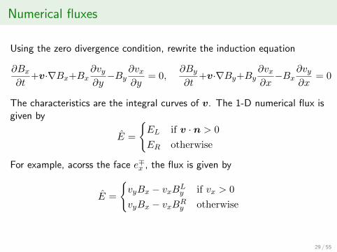
Numerical fluxes

Using the zero divergence condition, rewrite the induction equation

∂Bx

∂t+v·∇Bx+Bx

∂vy∂y−By

∂vx∂y

= 0,∂By

∂t+v·∇By+By

∂vx∂x−Bx

∂vy∂x

= 0

The characteristics are the integral curves of v. The 1-D numerical flux isgiven by

E =

EL if v · n > 0

ER otherwise

For example, acorss the face e∓x , the flux is given by

E =

vyBx − vxBL

y if vx > 0

vyBx − vxBRy otherwise

29 / 55

Numerical fluxes

BDL = (BDx , B

Ly ) BDR = (BD

x , BRy )

BUL = (BUx , B

Ly ) BUR = (BU

x , BRy )

The corner flux is given by

E =

EDL if vx > 0, vy > 0

EUL if vx > 0, vy < 0

EDR if vx < 0, vy > 0

EUR if vx < 0, vy < 0

which can be written in compact form as

E =vy2

(BUx +BD

x )− vx2

(BLy +BR

y )− |vy|2

(BU

x −BDx

)+|vx|2

(BR

y −BLy

)

30 / 55

Numerical fluxes

An equivalent expression is given by [11]

E =vy4

(BULx +BUR

x +BDLx +BDR

x )− vx4

(BULy +BUR

y +BDLy +BDR

y )

− |vy|2

(BUL

x +BURx

2− BDL

x +BDRx

2

)+|vx|2

(BUR

y +BDRy

2−BUL

y +BDLy

2

)

with the understanding that BDLx = BDR

x , etc.

31 / 55

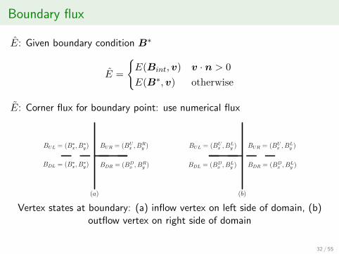
Boundary flux

E: Given boundary condition B∗

E =

E(Bint,v) v · n > 0

E(B∗,v) otherwise

E: Corner flux for boundary point: use numerical flux

BDL = (B∗x, B

∗y) BDR = (BD

x , BRy )

BUL = (B∗x, B

∗y) BUR = (BU

x , BRy )

(a)

BDL = (BDx , B

Ly ) BDR = (BD

x , BLy )

BUL = (BUx , B

Ly ) BUR = (BU

x , BLy )

(b)

Vertex states at boundary: (a) inflow vertex on left side of domain, (b)outflow vertex on right side of domain

32 / 55

Implementation details

0

4

1

5

8

10

9

11

2

6

3

7

Bx By

Mx 0 0 0 0 00 Mx 0 0 0 00 0 My 0 0 00 0 0 My 0 0Nx

l Nxr 0 0 Qx 0

0 0 Nyb Ny

t 0 Qy

33 / 55

Numerical Results

34 / 55

• Edge quadrature using (k + 2)-point GL rule

• Cell quadrature using (k + 2)× (k + 2)-point GL rule

• Time integration by 3-stage, 3-rd order SSPRK

• Time step

∆t <1

(2k + 1) max(|vx|∆x +

|vy |∆y

)• Code written using deal.II library

35 / 55

Test 1a: Approximation property

Take B = (∂xΦ,−∂xΦ) where

Φ(x, y) = sin(2πx) sin(2πy), (x, y) ∈ [0, 1]× [0, 1]

h ‖B −Bh‖L2(Ω) ‖div(Bh)‖L2(Ω)

0.1250 1.0189e-01 - 3.7147e-14

0.0625 2.5519e-02 2.00 9.5162e-14

0.0312 6.3826e-03 2.00 3.7880e-13

0.0156 1.5958e-03 2.00 1.4840e-12

0.0078 3.9896e-04 2.00 5.8016e-12

k = 1

h ‖B −Bh‖L2(Ω) ‖div(Bh)‖L2(Ω)

0.1250 6.7521e-03 - 1.3265e-13

0.0625 8.4659e-04 3.00 3.7389e-13

0.0312 1.0590e-04 3.00 1.3266e-12

0.0156 1.3241e-05 3.00 5.2716e-12

0.0078 1.6552e-06 3.00 2.0924e-11

k = 2

36 / 55

Test 1b: Approximation property

B = ∇Φ where

Φ(x, y) =1

10exp[−20(x2 + y2)], (x, y) ∈ [−1,+1]× [−1,+1]

h ‖B −Bh‖L2(Ω) ‖div(B)− div(Bh)‖L2(Ω)

0.0625 9.0930e-04 - 2.7438e-02 -

0.0312 2.2445e-04 2.02 6.9076e-03 1.99

0.0156 5.5927e-05 2.00 1.7299e-03 2.00

0.0078 1.3970e-05 2.00 4.3267e-04 2.00

0.0039 3.4918e-06 2.00 1.0818e-04 2.00

k = 1

h ‖B −Bh‖L2(Ω) ‖div(B)− div(Bh)‖L2(Ω)

0.0625 4.7750e-05 - 1.8703e-03 -

0.0312 5.9190e-06 3.01 2.3550e-04 2.99

0.0156 7.3827e-07 3.00 2.9491e-05 3.00

0.0078 9.2233e-08 3.00 3.6881e-06 3.00

0.0039 1.1528e-08 3.00 4.6106e-07 3.00

k = 2

37 / 55

Test 2: Smooth test case

The initial condition is given by B0 = (∂yΦ,−∂xΦ) where

Φ(x, y) =1

10exp[−20((x− 1/2)2 + y2)]

and the velocity field is v = (y,−x). The exact solution is a pure rotationof the initial condition and is given by

B(r, t) = R(t)B0(R(−t)r), R(t) =

[cos t − sin tsin t cos t

]Animation

38 / 55

Test 2a: Smooth test case

We compute the numerical solution on the computational domain[−1,+1]× [−1,+1] upto a final time of T = 2π at which time thesolution comes back to the initial condition.

(a) (b) (c)Contour of |Bh| for Test 2a, 10 contours between 0 and 0.3867: (a)

initial, (b) final, k = 1, (c) final, k = 2

39 / 55

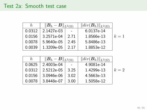
Test 2a: Smooth test case

h ‖Bh −B‖L2(Ω) ‖div(Bh)‖L2(Ω)

0.0312 2.1427e-03 - 6.0137e-140.0156 3.2571e-04 2.71 1.8566e-130.0078 5.9640e-05 2.45 5.8486e-130.0039 1.3209e-05 2.17 1.8853e-12

k = 1

h ‖Bh −B‖L2(Ω) ‖div(Bh)‖L2(Ω)

0.0625 2.4003e-04 - 4.9081e-140.0312 2.5212e-05 3.25 1.4299e-130.0156 3.0946e-06 3.02 4.5663e-130.0078 3.8448e-07 3.00 1.5058e-12

k = 2

40 / 55

Test 2b: Smooth test case

We compute the numerical solution on the computational domain[0, 1]× [0, 1] upto a final time of T = π/4.

(a) (b) (c)Contour of |Bh| for Test 2b, 10 contours between 0 and 0.3867: (a)

initial, (b) final, k = 1, (c) final, k = 2

41 / 55

Test 2b: Smooth test case

h ‖Bh −B‖L2(Ω) ‖div(Bh)‖L2(Ω)

0.0312 6.5882e-04 - 2.8687e-140.0156 1.4979e-04 2.13 9.8666e-140.0078 3.6394e-05 2.04 3.2902e-130.0039 9.0308e-06 2.01 1.1356e-12

k = 1

h ‖Bh −B‖L2(Ω) ‖div(Bh)‖L2(Ω)

0.0625 1.4110e-04 - 2.4986e-140.0312 1.7238e-05 3.03 7.9129e-140.0156 2.1442e-06 3.00 2.5910e-130.0078 2.6749e-07 3.00 9.2720e-13

k = 2

42 / 55

Test 3: Smooth test case, divergent solution

The exact solution is taken to be

B(x, y, t) =

[cos t − sin tsin t cos t

]B0(x, y)

where

B0 = ∇φ, φ =1

10exp(−20(x2 + y2))

so that ∇ ·B 6= 0, and the velocity field is taken as

v = ∇>ψ, ψ =1

πsin(πx) sin(πy)

The right hand side source term M is computed from the above solutionusing the formula M = −∂B

∂t +∇× (v ×B). The problem is solved onthe domain [−1,+1]× [−1,+1] until a final time of T = 2π.

43 / 55

Test 3: Smooth test case, divergent solution

(a) (b) (c)Contour plot of Bx for Test 3 showing 16 contours between -0.3838 and

+0.3838: (a) initial condition, (b) final, k = 1 and (c) final, k = 2

44 / 55

Test 3: Smooth test case, divergent solution

h ‖Bh −B‖L2(Ω) ‖div(B)− div(Bh)‖L2(Ω)

0.0312 8.5550e-04 - 6.9076e-03 -0.0156 1.8915e-04 2.17 1.7299e-03 1.990.0078 3.8730e-05 2.29 4.3267e-04 1.990.0039 7.8346e-06 2.30 1.0818e-04 1.99

k = 1

h ‖Bh −B‖L2(Ω) ‖div(B)− div(Bh)‖L2(Ω)

0.0625 3.4775e-04 - 1.8703e-03 -0.0312 3.3408e-05 3.38 2.3550e-04 2.990.0156 3.0287e-06 3.46 2.9491e-05 2.990.0078 2.7345e-07 3.47 3.6881e-06 2.99

k = 2

45 / 55

Test 4: Discontinuous test case

We take the potential

Φ(x, y) =

2y − 2x x > y

0 otherwise

and the velocity field is v = (1, 2). This leads to a discontinuous magneticfield with the discontinuity along the line x = y

B0 =

(2, 2) x > y

(0, 0) x < y

The exact solution is given by

B(x, y, t) = B0(x− t, y − 2t)

Animation

46 / 55

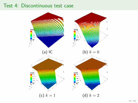
Test 4: Discontinuous test case

(a) IC (b) k = 0

(c) k = 1 (d) k = 247 / 55

Summary

• DG scheme on Cartesian meshes

• Globally divergence-free solutions

• Arbitrary orders possible

• Local mass matrices: good for explicit time-stepping

48 / 55

Ongoing work

• Adaptive mesh refinement

• Unstructured grids

• Limiters

• Application toI Maxwell equations (CED)I Magnetohydrodynamics (MHD)

Thank You

49 / 55

Ongoing work

• Adaptive mesh refinement

• Unstructured grids

• Limiters

• Application toI Maxwell equations (CED)I Magnetohydrodynamics (MHD)

Thank You

50 / 55

References

[1] C. R. Evans, J. F. Hawley, Simulation of magnetohydrodynamic flows -A constrained transport method, Astrophysical Journal 332 (1988)659–677.doi:10.1086/166684.

[2] D. S. Balsara, Divergence-free adaptive mesh refinement formagnetohydrodynamics, Journal of Computational Physics 174 (2)(2001) 614 – 648.doi:http://dx.doi.org/10.1006/jcph.2001.6917.URL http://www.sciencedirect.com/science/article/pii/

S0021999101969177

51 / 55

References

[3] F. Li, L. Xu, S. Yakovlev, Central discontinuous galerkin methods forideal MHD equations with the exactly divergence-free magnetic field,Journal of Computational Physics 230 (12) (2011) 4828 – 4847.doi:http://dx.doi.org/10.1016/j.jcp.2011.03.006.URL http://www.sciencedirect.com/science/article/pii/

S0021999111001495

[4] S. K. Godunov, The symmetric form of magnetohydrodynamicsequation, Num. Meth. Mech. Cont. Media 34 (1972) 1–26.

[5] K. Powell, An approximate Riemann solver for magnetohydrodynamics(that works in more than one dimension), Tech. Rep. 94-24, ICASE,NASA Langley (1994).

52 / 55

References

[6] P. Chandrashekar, C. Klingenberg, Entropy stable finite volume schemefor ideal compressible mhd on 2-d cartesian meshes, SIAM Journal onNumerical Analysis 54 (2) (2016) 1313–1340.arXiv:https://doi.org/10.1137/15M1013626,doi:10.1137/15M1013626.URL https://doi.org/10.1137/15M1013626

[7] A. Dedner, F. Kemm, D. Kroner, C.-D. Munz, T. Schnitzer,M. Wesenberg, Hyperbolic divergence cleaning for the MHD equations,Journal of Computational Physics 175 (2) (2002) 645 – 673.doi:http://dx.doi.org/10.1006/jcph.2001.6961.URL http://www.sciencedirect.com/science/article/pii/

S002199910196961X

[8] A. M. Quarteroni, A. Valli, Numerical Approximation of PartialDifferential Equations, 1st Edition, Springer Publishing Company,Incorporated, 2008.

53 / 55

References

[9] F. Brezzi, M. Fortin, Mixed and Hybrid Finite Element Methods,Springer-Verlag New York, Inc., New York, NY, USA, 1991.

[10] D. N. Arnold, D. Boffi, R. S. Falk, Quadrilateral H(div) finiteelements, SIAM Journal on Numerical Analysis 42 (6) (2005)2429–2451.arXiv:https://doi.org/10.1137/S0036142903431924,doi:10.1137/S0036142903431924.URL https://doi.org/10.1137/S0036142903431924

[11] D. S. Balsara, R. Kappeli, Von Neumann stability analysis of globallydivergence-free RKDG schemes for the induction equation usingmultidimensional riemann solvers, Journal of Computational Physics336 (2017) 104 – 127.

54 / 55

References

doi:https://doi.org/10.1016/j.jcp.2017.01.056.URL http://www.sciencedirect.com/science/article/pii/

S0021999117300724

55 / 55