A Global VAR Model for the Analysis of

Wheat Export Prices

Luciano Gutierrez

Dipartimento di Agraria, University of Sassari, Italy ∗

Francesco Piras

Dipartimento di Agraria, University of Sassari, Italy.

Abstract

Reasonable limited volatility is a common feature of agricultural markets, particularly in

international markets. However, occasionally, more pronounced and even extreme upward or

downward price spikes have been recently registered. Food commodity prices fluctuations has

important impacts on poverty and food insecurity across the world. Conventional models have

not provided a complete picture of recent price spikes in agricultural commodity markets, while

there is an urgent need for appropriate policy responses. Perhaps new approaches are needed

in order to better understand international spill-overs, the feedback between the real and the

financial sectors and also the link between food and energy prices. In this paper, we present

results from a new worldwide dynamic model that provides short and long-run impulse responses

of wheat international price to various real and financial shocks. The results show that stocks, oil

price and US dollar depreciation affect worldwide wheat prices.

Keywords: Global Dynamic Models, Price analysis, Wheat market.

JEL Classification: G14, Q14, C12, C15.

∗Corresponding author: Telephone: +39.079.229.056, Fax: +39.079.229.356, E-mail address: lgutierr@uniss.it.

1

1 Introduction

During the food crisis of 2006-2008 and 2010-2011 the world observed large increases in the prices ofwheat, rice and maize on international markets. The surges in prices on international markets ledto substantial increases in domestic prices. According to FAO 1 by July 2008, domestic wheat, rice,and maize prices where each, on average among countries, about 40% higher (adjusted for inflation)than they were in January 2007. Although, in recent years numerous factors have been proposedin the literature as explaining recent commodity price movements, there is no general consensus onthe relative weight that should be attributed to each of them. Many authors have stressed that moreconsideration should be given to the effects of growing food demand in developing countries, especiallyin China and India, and also to the lower production growth rate as being among the causes of therecent food price spike (see for example Trostle, 2008; Von Braun, 2007; Dewbre et al. 2008, andKrugman, 2011). Other studies have argued that biofuel programs in the United States and EuropeanUnion are behind the run-up in food prices. These programs provide subsidies for biofuels leadingto greater use of corn and vegetable oil and resulting in price increases for these commodities (seeMitchell, 2008 and Headey and Fan, 2008). On the other hand Baffes and Haniotis (2010) suggestedthat the link between food prices and energy prices is the main factor in recent commodity pricemovements. Energy prices affect food commodity prices by influencing the cost of inputs, such asnitrogen fertilizer, and the cost of transport. The use of agricultural commodities to produce biofuelsis also an additional reason for a possible link between energy and food commodity prices. Besidesthe above mentioned factors, the list of possible causes analysed in the recent literature includes thedecline of commodity stocks (Abbot, Hurt and Tyner, 2008; Piesse and Thirtle 2009), a weak U.S.dollar (Abbot, Hurt and Tyner, 2008; Mitchell, 2008), panic buying (Timmer, 2009), bans on exports(Dollive, 2008; Headey, 2011) and speculation (Irwin, Sanders and Merrin, 2010; Cooke and Robles2009; Sanders, Irwin and Merrin, 2010; Gilbert, 2010a; 2010b; Gutierrez, 2013).

The aim of the paper is to model the impacts of the main factors behind the wheat export pricedynamics. In details, the research provides a worldwide dynamic model for the analyses of short andlong-run impulse responses of wheat commodity prices to various real and financial shocks. Specifically,we propose a GLObal Wheat Market Model (GLOWMM) to study the dynamic of wheat export prices.The model is specified by using the Global Vector AutoRegressive (GVAR) model proposed by Pesaranet al. (2004) and Dees et al. (2007). The methodology allows the analysis of wheat export prices forthe six main export countries, USA, Argentina, Australia, Canada, Russia and EU. Specifically, singlecountry wheat export prices are modelled as persistence processes that reverts to a time-varying meandetermined by both country-specific and foreign-specific variables plus the effect of global variables,as the oil price. These single country models are then aggregated into a global model by using exportweighting matrices. Thus we can evaluate the first and second round inflationary effects on wheatexport prices of various shocks as a reduction of the wheat stock to utilization ratio, an increase inthe oil price and a US currency devaluation relative to the main competitor’s currencies.

The paper is organized as follows. Section 2 provides the motivation for this study and describesthe econometric model. In Section 3 data and empirical results are discussed. Section 4 concludes.

2 Motivation and methodology

Amid the recent food commodity prices turmoil, policy makers have become increasingly concernedon what happened (and why) on world food markets in recent years. As shown in Figure 1 whichreports the FAO Food Price Index, food prices have increased abruptly since 2002 and especially sincelate 2006 leading to unprecedented highs between 2006 and 2008. In the second half of 2008 pricesdeclined again but market turbulence returned in late 2010 recalling back the negative memories of2008 crises (Tangermann, 2011; Serra and Gil, 2012).

A wide strand of different explanations for recent food prices increased volatility has been proposedin the literature. The identification of the main factors is still under debate. Obviously it is not aneasy task to depict a clear picture of food price crisis because it is a global phenomenon that involves alarge number of distinct events. Many authors have considered some explanations more reliable thanothers.

Figure 1 about here

1FAO Global information and Early a Warning System

2

Unfavourable weather condition in major producing countries have been viewed as one importantfactors according to OECD report (2008), Tangermann (2011) and OECD-FAO (2011). Despite ofthis, Headey and Fan (2008) suggest that production shortfalls are a normal occurrence in agriculturaland low production in several countries were offset by large crop in other regions. Macroeconomicconditions such as strong GDP growth and subsequent stronger demand for food in some developingcountries have also been considered as a permanent factor behind the recent prices spike (see VonBraun, 2007; Trosle, 2008; Carter et al., 2011; Krugman, 2011). Other studies have argued that lowlevel of real interest rates and growing money supply diverted investments away from financial assetstowards physical assets, including commodities. This excess of liquidity in the global economy, witha depreciation of US dollar, resulted in inflation and in its turn, in rising commodity prices and anincreased commodities demand for importing countries (see Calvo, 2008; Abbot et al. 2008; Mitchell,2008; Timmer, 2009; Gilbert, 2010a; Tangermann 2011).

The excess of liquidity fostered financial investments in commodity future markets convincingsome authors that speculation and not fundamentals were behind the commodities price boom andbust (Baffes and Haniotis, 2010; Masters, 2008; Soros ,2008; Calvo, 2008). Cooke and Robles (2009),Gilbert (2010b) and Gutierrez (2013) found evidences that financial activities in future markets maybe of use in explaining the change in food price. However, a large strand of literature challengedthe arguments proposed by the bubble proponents through logical inconsistencies, conceptual errorsand empirical evidences showing that speculation did not have a significant role in rising commoditiesfood prices (see Krugman, 2009; Wolf, 2008; Wright, 2009; Irwin et al., 2009; Sanders and Irwin,2010; Baffes and Haniotis, 2010). Other possible causes analysed in literature include the decline ofcommodity stocks, the rising of crude oil price, biofuels production and finally panic buying, ban andexport restrictions.

The competitive storage model explains how commodity stocks can play a main role in bufferingprice volatility (see the pioneering work of Gustafson 1958; but also Samuelson 1971; Wright andWilliams 1982; Scheinkman and Schechtman 1983; Williams and Wright 1991 and Deaton and Laroque1992). Starting on the years 1999-2000, the global stock level for major cereals has been declinedreaching its historical low level in 2007 (Dawe, 2009; Wright, 2011; Tangermann, 2011). Therefore, itis not surprising that literature has identified the reduction of commodity stocks as one of the mainfactors in recent food price spike (Piesse and Thirtle, 2009; Trostle, 2008; Dawe, 2009). Empiricalevidence have been provided by Kim and Chavas (2002), Balcombe (2011), Carter et al. (2011),Hochman et al. (2011), Serra and Gil (2012). The oil price represents a permanent factor in foodprice formation and some authors have highlighted its possible importance as major factor in therecent prices boom (see Baffes, 2007; Baffes and Haniotis, 2010; Balcombe, 2011, among others).Moreover, as oil price increases, biofuels becomes more competitive. Mitchell (2008), Baffes (2007),OCSE-FAO (2011) and Tangermann (2011) suggest that biofuels contributed to the price crisis in2006-2008. Hochman et al. (2011) provide a complete literature about quantitative estimates ofbiofuels impact on food commodity price index.

In the paper, we focus on wheat market for two reasons. First rising food prices mainly affects lowerincome consumers, especially in poor countries where households spend a great part of their income onfood. This is particular true for cereals and especially wheat. It represents the most relevant sourceof food in developing countries. Second, market assumptions for the analysis of wheat are deeplychanged during the last decades evolving from an oligopoly between US and Canada with the latteras a price leader (McCalla, 1966) to a tripoly including also Australia (Alouze et al. 1978) and henceto a price leadership model with US price leader (Oleson 1979; Wilson, 1986). However, Westcott andHoffman (1999) recognize that although US is the largest word wheat exporter its market share is notenough to be considered a price leader anymore. In essence, wheat market is nowadays characterizedby a relative small number of wheat producing and exporting countries that sell to a relative largegroup of importers, mostly developing countries. While new market assumptions can be introducedfor example in general equilibrium models, more flexible models can be provided and used for theanalysis of worldwide commodity markets.

To this end, in this paper we introduce and evaluate an innovative econometric methodologyrepresented by the Global Vector Autoregressive model. The GVAR approach is particular appealingfor the analysis of the worldwide wheat market for two reasons. First, it is specifically designed tomodel fluctuations and interactions between countries. This is a crucial asset given the features ofworld wheat market and the global dimension of the food prices crisis that cannot be downsized to onecountry, rather involves a large number of countries. Secondly, the GVAR allows to model the dynamic

3

of wheat export prices as results of the effects exerted by the country-specific and by foreign-specificvariables. The foreign-specific variables are defined as weighted average of wheat export prices, thestock to utilization ratio and the effective exchange rate fluctuations in all competitor countries. Thusboth country-specific and foreign-specific effects can be jointly modelled. Finally the GVAR modelcombines a number of atheoretic relationships. Unlike structural models, as for example generalequilibrium models, the approach does not attempt to make restrictions, for example on the basis ofeconomic theory. Causal relationships are analyzed by means of the impulse response functions that,built from the GVAR estimates, allow to highlight how shocks on wheat stocks and demand, exchangerates, input prices or global oil price propagate at domestic and global level.

2.1 The analytical framework

Before presenting the GVAR methodology, it is useful to introduce a simple model which may accountfor the main relationships among the dynamics of export prices, cost prices, stock and demand factorsand exchange rates. For each country the export price equation can be derived for example within amark-up framework. Oligopolist behaviour in wheat international market has been largely analyzedin many study as McCalla(1966), Alouze et al. (1978), Oleson (1979), Wilson, (1986), Arnade andPick (1997) and more recently Arnade and Vocke (2013). Setting-up the model, we assume that thelog of export prices expressed in US dollar in country i for i = 0, ..., N and at time t for t = 1, ..., T ,pxit, is set as mark-up mkit on the marginal production cost, cpit (expressed in log)

pxit = (1 +mkit) + cpit + εit. (1)

Using a pricing to market strategic behaviour (Krugman, 1987; Knetter, 1992; Athukorala and Menon,1994 among others), the mark-up in each country i is hypothesised to depend on the competitivepressure in the world market and stock and demand pressures in both the home and world market.These effects can be modelled by the following equations

mkit = mk

∑j =i

wj

(pxl

jt − ejt)−

(pxl

it − eit) (2)

pxlit = pxl (zit, Sit) . (3)

In equation (2) the mark-up depends on the ratio between the price of competitors given by theaverage of competitors’ prices weighted by the share, wj , that each country has in the world exportmarket, and the home price. In order to include the effects of exchange rates, the export price pxit

is defined as ratio of the home price expressed in local currency, pxlit, and the log of the bilateral

exchange rate of local currency in country i per unit of US dollar. Finally, in equation (3)the homeprice is assumed for each country i to depend on the supply and demand effects synthesised in thestock to utilization ratio variable, zit, an other variables which may affect home prices defined bythe variables Sit. Substituting (2) and (3) in (1) and assuming a linear relationship among the logvariables, it easily to see that the export price equation can be expressed as

pxit = α+ β1cpit + β2eit + β3zit + β4Sit + β5e∗t + β6z

∗t + β7S

∗t + εit. (4)

where e∗t =∑

j =i wjejt, z∗t =∑

j =i wjzjt and S∗t =

∑j =i wjSjt. From (4) emerges that export

prices are influenced by a set of home variables and a set foreign variables computed as average ofthe exchange rates, e∗t , the average stock to use ratio, z∗t and other variables S∗

t which all accountfor the effects of external competitors’ factors on the dynamics of countries export prices. Similarequation can be derived for the stock to use variable zit. The original feature of the GVAR modellingapproach lies in the ability to estimate models expressed in the form (4). Specifically, the GVARmodel is basically composed of a number of countries modelled individually and estimated as a vectorautoregression and the dynamics of home variables are linked each others by including foreign-specificand global variables related to the international export patterns of each country. The specification ofthe GVAR model proceeds in two stages. In the first stage, i.e. the estimation stage, the reduced formvector autoregression VAR model, augmented with the exogenous, X, variables, labelled VARX(p, q),is estimated for each country i, and in the second stage all individual country VARX models arestacked and linked using weight matrices.

4

Specifically, modelling each country i as a VARX(p, q),

Φi (L, pi) yit = ai0 + Λi (L, qi) y∗it +Ψi (L, qi) dt + ϵit (5)

where the indexes i = 1, ..., N ; t = 1, ..., T , ai0 is a (ki × 1) vector of deterministic intercepts, yit is a(ki × 1) vector of country-specific (domestic) variables and corresponding (ki × ki) matrices of laggedcoefficients, denoted by Φi (L, pi) = I−

∑pi

p=1 ΦiLi, where L is the lag operator; y∗it is a (ki × 1) vector

of trade-weighted foreign variables and corresponding (ki × k∗i ) matrix of lag polynomial denoted byΛi (L, qi); Ψi (L, qi) is a matrix lag polynomial associated to the global exogenous variables dt. Finallyϵit is a (ki × 1) vector of zero mean, idiosyncratic country-specific shocks, assumed to be seriallyuncorrelated and with time invariant covariance matrix

∑ii, i.e ϵit ∼ iid (0,

∑ii). The GVAR model

assumes the weak exogeneity of y∗it, i.e. the models rules out long-run feedbacks from yit to y∗it.The first step of the analysis is to fix the order of the matrices polynomial Φi (L, pi), Λi (L, qi) and

Ψi (L, qi). We use the Akaike information criterion (AIC). We allow at maximum for a VARX(3, 1),the maximum pi allowed is pi = 3 and qi is qi = 1 in order to reduce the number of estimatedparameters and avoid degrees of freedom problems. In the second stage of the GVAR methodology,we cast the country-specic models into their global representation. To show how the GVAR model isconstructed, consider a generic country i in (5) with pi = 2 and qi = 2 and assume that Ψi (L, qi) = 0

yit = ai0 +Φi1yit−1 +Φi2yit−2 + Λi0y∗it + Λi1y

∗it−1 + Λi2y

∗it−2 + εit. (6)

First, for each country we group both the domestic and foreign variables as

zit =

(yity∗it

), (7)

Therefore each country VARX model (6) becomes

Aizit = ai0 +Bi1zit−1 +Bi2zit−2 + εit (8)

whereAi = (Iki ,−Λi0) , Bi1 = (Φi1,,Λi1) , Bi2 = (Φi2,,Λi2) . (9)

The next step we create a vector of variables

yt =

y0ty1t...

yNt

, (10)

and using the weight matrix Wi constructed as the export weights of each country relative to theexport of all competitor’s countries, we obtain the following identity

zit = Wiyt ∀i = 0, 1, ..., N. (11)

The previous relationship allows each country model to be written in terms of the global vector yt ,thus it is the fundamental device through which each country wheat market is linked to the globalGVAR model. Using now the identity (11) in each country VARX model (9) we obtain

AiWiyit = ai0 +Bi1Wiyit−1+Bi2Wyit−2 + εit. (12)

Finally by stacking each country-specific model in (12), we end with the Global VAR for all endogenousvariables in the system yt,

Gyit = ai0 +H1yit−1 +H2yit−2 + εt (13)

where

G =

A0W0

A1W1

.

..ANWN

, H1 =

B01W0

B11W1

.

..BN1WN

, H2 =

B02W0

B12W1

.

..BN2WN

, a0 =

a00a10...

aN0

, εt =

ε0tε1t...

εNt

.

If the G matrix is non singular, it can be inverted obtaining the Global VAR model in its reduced

5

form, i.eyt = b0 + F1yt−1 + F2yt−2 + vt (14)

where

F1 = G−1H1, F2 = G−1H2, b0 = G−1a0, vt = G−1εt.

3 The empirical results

In the application, we employ data for the main six wheat export countries: Argentina, Australia,Canada, Russia, EU and USA at monthly frequency for the period July 2000 to January 2012. TheGVAR model includes five variables for each country-specific VARX model: the wheat export pricespeit, expressed in US dollars, the home wheat stock to utilization ratio zit, the fertilizer price pfitexpressed in US dollars. We first build the indexes of all variables using the period (July/2000-June/2001)=100 as the base year.

The fluctuation of the exchange rate influences the dynamic of export prices. As previously intro-duced the GVAR model accounts for the effects of country-specific and foreign-specific variables.

Thus the foreign-specific variables are constructed as (geometric) average of the single countryvariables using as weights the export-country shares. The weights are presented in Table 1. Thechoice of weights based on exports is undertaken with the rationale that exogenous shocks, as a wheatstock reductions or and exchange rate devaluation, could pass-through on export prices in all countriesthrough the trade channel. We use fixed weights over time computed as average of the years 2008-2010. Data are from the International Grain Council. Thus, both country-specific and foreign-specificvariables will affect the system. As for the exchange rate, wheat export prices in a specific countrywill be influenced by home variables as the stock to utilization ratio, the deflated exchange rate, thedynamics of fertilizer input prices and by the foreign-specific variables given by the average wheatstocks to utilization ratio, z∗it, the rer∗it variable, the average wheat foreign prices pe∗it .

Table 1 about here

Finally, the home wheat export prices will be also influenced by global variables, i.e. variablescommon to all countries, as the oil price pot . All variables, with the exception of the stock to utilizationratio, are log transformed. In the Data Appendix we present the data sources and the key steps usedfor their analysis.

The first step in the analysis is to test the nonstationary properties of our series.2 The resultsare presented in Table (2). Given that the majority of the series are I(1), the cointegrating VARXcountry models are estimated subject to the reduced rank restriction (Johansen, 1992 and 1995).

Table 2 about here

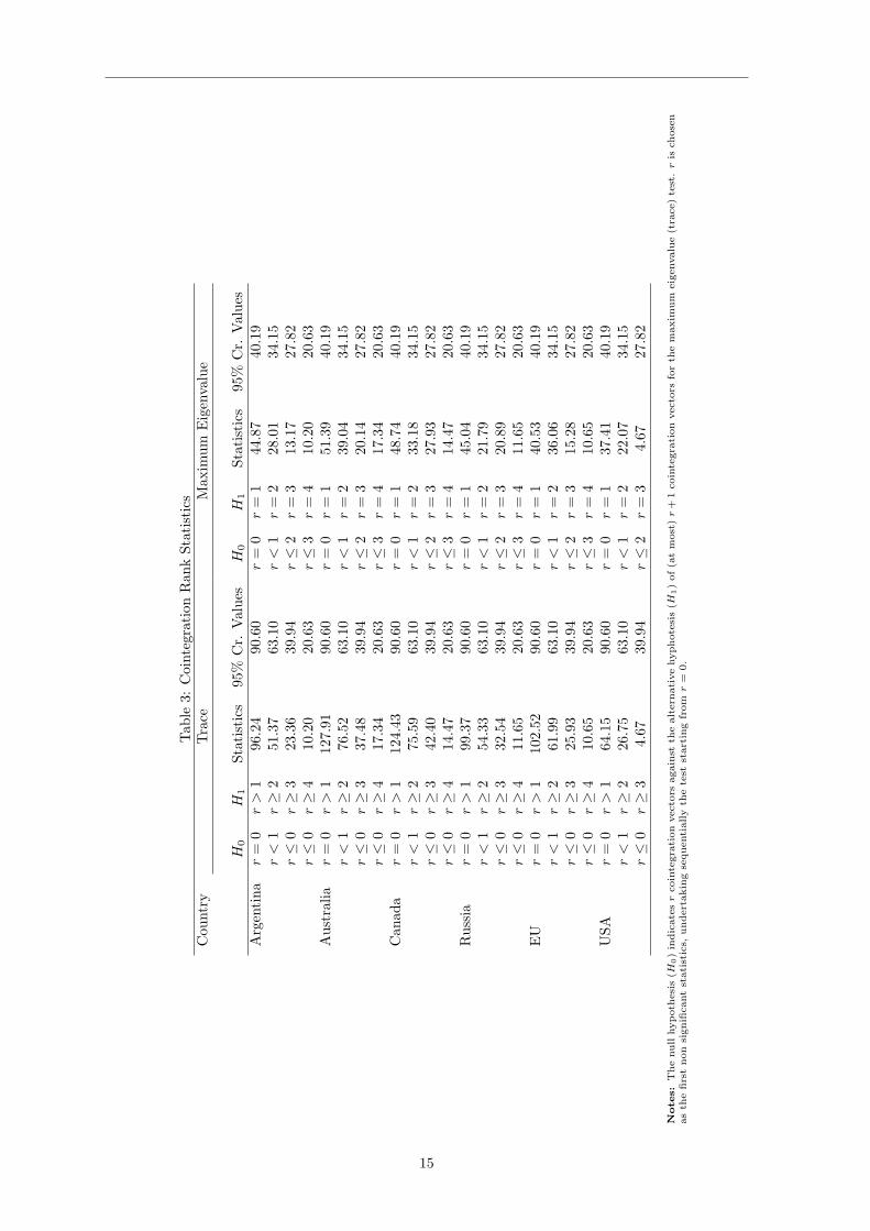
To this end we employ the trace and maximum eigenvalue statistics. Both tests are conducted atthe 95% significance level when a restricted intercept is included in the model. The rank statistics arereported in Table (3), while the number of cointegrating relationships for each VARX country modeland the VARX autoregressive orders p, q are reported in table (4). The VARX orders are estimatedusing the Akaike criterion. For all country models, with the exception of Australia, the rank testssuggest one cointegration relation. For Australia, both tests indicate the presence of two cointegratingrelations. Thus, each country model has been estimated using its Vector Error Cointegration (VEC)form or, in other words, each country model is estimated subject to reduced rank restriction.

Table 3 about here

Table 4 about here

The estimation of the cointegrating VEC models gives the opportunity to analyze the effects offoreign variables on their home counterparts. Specifically, the model allows for the analysis of theimpact on the home variables of a 1% change of the corresponding foreign-specific variables. Theseimpacts have been labelled as impact elasticities and permit the analysis of the co-movements among

2All the procedures for the analysis of the GVAR model have been written using GAUSS 11.

6

the home and foreign variables. In table (5), we present the impact elasticities and their t-statistics.Looking at wheat export prices, we find that all the estimates are positive and significant, with theexception of Russia estimate that it is not significant at the 5% significance level. Moreover, USA,Canada and Australia show an impact elasticity close to one. Positive but mainly non significantco-movements are evidenced by the real exchange rate variable. EU is the only region that shows apositive an significant estimate. Finally the stock-to utilization ratio variable presents both positiveand negative co-movements. Argentina reports a negative and significant correlation, the elasticityfor Russia is negative but not significant. However, the elasticities are positive and significant for theremaining countries.

Table 5 about here

The GVARmodel requires to account for the hypothesis of weak exogeneity for both the foreign andglobal variables. We use the exogeneity test proposed by Johansen (1992). For each country-specificmodel, the following regression is performed

∆yit,l = µil +

ri∑j=1

γij,lECM ji,t−1 +

pi∑k=1

ϕik,l∆yi,t−k +

qi∑m=1

θik,l∆yi,t−m + ϵit,l (15)

where the ∆yi,t−k is the group of home variables expressed in differences, with k = 1, ..., pi and piis the lag order of the home component for each of ith country model, ∆yi,t−m is the set of foreign-specific and global variables in differences, with m = 1, ..., q and q is the lag order of the foreign-specificand global components for each of ith country model, and finally ECM j

i,t−1 is the estimated errorcorrection term, with j = 1, ..., ri, and ri is the number of cointegrating relations, i.e. the rank, foundin the ith country model. The procedure consists in testing by means of an F the joint hypothesisthat γij,l = 0 for each j = 1, ..., ri. Results of Table 6 indicate that the hypothesis of weak exogeneitycannot be rejected.

Table 6 about here

4 Generalized Impulse Response Analysis

In the absence of strong a priori information to identify the short-run dynamics of our system, we usethe generalised impulse response function (GIRF) approach proposed in Koop, Pesaran and Potter(1996) and further developed in Pesaran and Shin (1996). The GIRF has the nice property of beinginvariant to the ordering of the variables and of the countries. This is of particular importance inour system where there is not a clear economic a priori knowledge which can establish a reasonableordering. To assess the dynamic properties of the GVAR model and the time profile of the effects ofshocks to home foreign variables, we analyze the implications of five different external shocks:

• A one standard error negative shock to US stock to utilization ratio

• A one standard error negative shock to global stock to utilization ratio

• A one standard error positive shock to oil price

• A one standard error negative shock to real effective exchange rate

• A one standard error positive shock to fertilizer price

Due to space limitation we only present the GIRF impulse responses of the wheat export pricesfor the various countries analyzed and we focus on the first two years following the shock.

The first shock we consider is a negative shock to the USA stock to utilization ratio. In this casea one-standard deviation shock corresponds to a decrease of 0.11% of the value of the variable.3 InFigure 2, we show the effect of this shock on the wheat export prices with the solid line, while the 90%bootstrapped confidence intervals are represented by the thinner lines 4. Unsurprisingly, a negativeshock to US stock to utilization ratio raises the export prices in all countries. In US the response

3During the period of analysis, the average value of the variable is 0.511.4The confidence interval is calculated using the sieve bootstrap method with 1000 replications.

7

impact is +1.6%, after three months the wheat export price reaches the maximum of +4.9%. Similarshapes are evidenced by other countries. Argentina, Australia, Canada show similar impacts after thestock to utilization ratio shock, while Russia and EU present minor impact with long-run increase ofwheat export prices of +2.0%.

Figure 2 about here

The second shock we analyze is what can be labelled the perfect storm of the stock to utilizationratio variable. We simulate a decrease of this variable in all countries, i.e. we assume a general reduc-tion in stock detained by the main export countries. The one-standard deviation shock correspondsin this case to an average decrease of 0.14%5. The impact on export prices is shown in Figure 3. Asexpected, the contemporaneous effect on wheat export prices is relevant. The export prices raise fromthe minimum value of +1.3% in Argentina to the maximum value of +3.0% in USA. Second-roundeffects are also relevant. Export prices in the first rapidly increase reaching values that ranges from+6.6% in Canada to +13.1% in Russia before reducing in the following months.

Figure 3 about here

The devaluation of the US exchange rate has been ascribed as one of the main factors behindthe commodity prices upsurge during the period 2007-2008. For this reason we simulate the effectof reduction on the rer∗it variable that can be interpreted as a global (real) devaluation of the USexchange rate. A one standard error shock in this case is equivalent to a fall of around 15% of the USdollar against the competitors’ currencies. Interestingly, the shock is accompanied by a raise of wheatexport prices of the same entity. Thus, with the exception of Argentina and Australia that show alower impact, on average we note an unitary elasticity of wheat export prices to a devaluation.

Figure 4 about here

In Figure 5 are presented the impulse responses of a one standard error shock on the fertilizerprice. In this case the one standard error shock means a raise of fertilizer price of 19.4%. Thisincrease is associated with an increase in wheat export prices of 1.4%. The full effect after 24 monthsis differentiated. Russia and EU show the same long-run impact +7%, the long-run impact for USAremains at a baseline of 4% and for the other countries the magnitude of the rate of growth of wheatprices remains limited between 1% and 2%.

Figure 5 about here

We finally analyze the effect of a global oil price shock to the dynamics of the export prices. Theresults are reported in Figure 6. A positive standard error unit shock to nominal oil prices correspondsto an increase of about 8.6 percent of the oil price index in one month. The impact of wheat exportprices vary significantly among countries. For US and EU area the impact is quite similar and equalto 1.0%. Australia is the country that seems to suffer more for an oil shock with an impact on wheatexport price close to 1.5%.

Figure 6 about here

5 Concluding Remarks

In this paper, we have employed the Global Vector Autoregressive (GVAR) methodology for theanalysis of short and long-run response of wheat export prices to both different country-specific andcommon shocks. Impulse response analysis reveals that a decrease of wheat stocks with respect to thelevel of consumption, and increase of oil prices and real exchange rate devaluation have all inflationaryeffects on wheat export prices although their impacts are different among the main export countries.Unfortunately by construction the model is nonstructural. Structural interpretations of VAR modelsrequire additional identifying assumptions that must be motivated mainly on institutional knowledge,economic theory, or other constraints on the model responses. Only after having identified the modelwe can assess the causal effects of all previous shocks on the model variables. However this work canbe done using the approach proposed by Dees et al. (2007), and we leave this for future research.

5This value has been obtained as using single countries export shares

8

Acknowledgement

An earlier version of this paper was presented at the University of Ceara, Brasil, at the MACSURWorkshop on ”TradeM: New Ideas for Model Integration”; University of Haifa, Israel and at the SpecialSession entitled ”Integrated modelling of climate impacts on food and farming at regional to supra-national scales”, UNCCD 2nd Scientific Conference, Bonn Germany. We thank participants of thesessions for their valuable comments and suggestions. The research was supported by a MIUR grantand research funds from the Italian Ministry of Agriculture under the project MACSUR, ”ModellingEuropean Agriculture with Climate Change for Food Security”.

9

References

Abbott, P.C., Hurt, C. and Tyner, W.E. (2008). Whats driving food prices? Issue Report, FarmFoundation, June 2008.Alaouze, C.M., Watson A.S., Sturgess N.H. (1978). Oligopoly Pricing in the World Wheat Market.American Journal of Agricultural Economics 60, 2: 173-85.Arnade C. and Pick D. (1999). Alternative Approach to Measuring Oligopoly Power: A Wheat MarketExample, Applied Economic Letters, 6: 195-198.Arnade C. and Vocke G. (2013). Investigating the Divergence in Wheat Prices. Paper presented atAAEA & CAES Joint Annual Meeting, Washington, D.C., 4-6 August 2013.Baffes, J. and Haniotis, T. (2010). Placing the 2006/08 commodity price boom into perspective.Policy Research Working Paper 5371, The World Bank Development Prospects Group, Washington,DC: World Bank.Baffes, J. (2007). Oil spills over into other commodities.Policy Research Working Paper, WashingtonD.C.: World Bank 2007.Balcombe, K. (2011). Safeguarding food security in volatile global markets, chapter 5, FAO; Rome2011, edited by Adam Prakash.Calvo , G. (2008). Exploding Commodity Price, Lax Monetary Policy, and Sovereign Wealth Funds.VOXEU, June 20, 2008.Carter, C.A., Rausser, G.C., Smith, A. (2011), Commodity Booms and Busts, The Annual Review ofResource Economics, 2011. 3:87-118.Cooke, B. and Robles, M. (2009). Recent food price movements: A time series analysis. DiscussionPaper n. 00942, International Food Policy Research Institute (IFPRI), December 2009, Washington,DC: IFPRI.Dawe, D. (2009), The Unimportance of Low World Grain Stocks for Recent World Price Increases.Agricultural and Development Economics Division (ESA) Working Paper 09-01. Rome: Food andagriculture Organization.Deaton, A., Laroque, G. (1992). On the behaviour of commodity prices, Review of Economic Studies,59(1):1-23.Dees, S., Di Mauro, F., Pesaran, M.H. and Smith, L.V. (2007). Exploring the international linkagesof the euro area : a global VAR analysis.Journal of Applied Econometrics, 22(1): 1-38.Dewbre, J., Giner, C., Thompson W. and Von Lampe M. (2008). High food commodity prices: Willthey stay? Who will pay? Agricultural Economics 39: 393-403.Dollive, K. (2008). The Impact of Export Restraints on Rising Grain Prices. Office of EconomicsWorking Paper No. 2008-08-A, US International Trade Commission, Washington, DC.Gilbert, C. (2010a). How to Understand High Food Prices. Journal of Agricultural Economics 61:398-425.Gilbert, C. (2010b). Speculative influences on commodity futures prices 2006-2008, Discussion papersn. 197, United Nations Conference on Trade and Development(UNCTAD), New-York: UNCTAD.Gustafson, R. (1958). Carryover levels for grains, Washington DC:USDA, Technical bulletin 1178.Gutierrez, L. (2013), Speculative bubbles in agricultural commodity markets. European Review ofAgricultural Economics, 40(2):217-238.Headey, D. (2011). Rethinking the global food crisis: The role of trade shocks, Food Policy 36:136-146.Headey, D., and Fan, S. (2008). Anatomy of a crisis: the causes and consequences of surging foodprices, Agricultural Economics 39: 375-391.Hochman, G., Rajagopal, D., Timilsina, G., Zilberman, D. (2011). The Role of Inventory Adjustmentsin quantifying Factors Causing Food Price Inflation. World bank. Policy Research Working Paper5744, August 2011.Irwin, S. H., Sanders, D.R. and Merrin R. P. (2010). Devil or Angel? The Role of Speculation inthe Recent Commodity Price Boom (and Bust), Journal of Agricultural and Applied Economics 41:377-391.Irwin, S. H., Garcia, P., Good, D.L. and Kunda, E.L. (2009). Poor convergence performance ofCBOT corn, soybean and wheat futures contracts: Causes and solutions, Marketing and OutlookResearch Report 2009-02, Department of Agricultural and Consumer Economics University of Illinoisat Urbana-Champaign.Johansen, S. (1992). Cointegration in Partial Systems and the Efficiency of Single-Equation Analysis.Journal of Econometrics, 52, 231-254.

10

Johansen, S. (1995), Likelihood-Based Inference in Cointegrated Vector Autoregressive Models, OxfordUniversity Press, Oxford.Kim, K. and Chavas, J. P. (2002). A dynamic analysis of the effects of a price support program onprice dynamics and price volatility. Journal of Agricultural and Resource Economics 27: 495514.Knetter M. (1987). International Comparisons of Pricing to Market Behavior. NBER Working PaperNo 4098.Koop, G., Pesaran, M.H. and S. Potter (1996). Impulse Response Analysis in Nonlinear MultivariateModels, Journal of Econometrics, 74, 119-147.Krugman, P. (1987). Pricing to Market when the Exchange Rates Changes, S.W. Arndt and J.D.Richardson,eds., Real-Financial Linkages Among Open Economies, Cambridge: MIT Press.Krugman, P. (2009) More on Oil and Speculation. New York Times, May, 13 2008.Krugman, P. (2011). Soaring food prices. New York Times, February, 5 2011.Masters, M. W. (2008). Testimony Before the U.S. Senate Committee of Homeland Security andGovernment Affairs. Washington DC, 20 May 2008.McCalla A.F. (1966). A Duopoly Model of World Wheat Pricing. Journal of Farm Economics 4, no.3:711-27.Mitchell, D. (2008). A note on rising food prices. Policy Research Working Paper 4682, Washington,DC: World Bank.Ng, S., and P. Perron (2001). Lag Length Selection and the Construction of Unit Root Tests withGood Size and Power. Econometrica 69, 1519-1554.OECD (2008). Rising Food Prices Causes and Consequences. Policy Report, 2008.OECD-FAO (2011), Agricultural Outlook 2011-2020. Paris: OECD.Oleson, B.T. (1979). Price Determination and Market Share Formation in the International WheatMarket. Unpublished Ph.D. dissertation. St. Paul: University of Minnesota, Department of Agricul-tural Economics.Piesse, J., and Thirtle, C. (2009). Three bubbles and a panic: An explanatory review of recent foodcommodity price events. Food Policy 34: 119-129.Pesaran, M.H., Schuermann, T., Weiner, S. (2004). Modelling Regional Interdependencies using aGlobal Error-correcting Macroeconometric Model, Journal of Business and Economics Statistics 22:129-162.Pesaran, M.H. and Shin (1996). Cointegration and Speed of Convergence to Equilibrium, Journal ofEconometrics, 71, 117-143.Samuelson, P. (1971). Stochastic speculative price, Proceedings of the National Academy of Sciences,68(2): 335-337.Sanders, D.R., Irwin, S. H., and Merrin, R.P. (2010). The Adequacy of Speculation in AgriculturalFutures Markets: Too Much of a Good Thing? Applied Economic Perspectives and Policy, 32: 77-94.Sanders, D.R., and Irwin, S. H. (2010). A speculative bubble in commodity future prices? Cross-sectional evidence. Agricultural Economics 41: 25-32.Scheinkman, J., Schechtman, J. (1983). A simple competitive model with production and storage.Review of Economic Studies, 50: 427-441.Serra T., Gil J.M., (2012). Price volatility in food markets: Can stock building mitigate price fluctu-ations? European Review of Agricultural Economics, 1-22.Soros G., (2008). Testimony before the U.S. Senate Commerce Committee Oversight: hearing onFTC Advanced Rulemaking on Oil Market Manipulation. Washington, D.C., June 3Tangermann, S. (2011), Policy Solutions to Agricultural Market Volatility: A Synthesis. ICTSD June,2011.Timmer, C.P. (2009). Did speculation affect world rice prices? ESA Working Paper n. 09-07, Foodand Agricultural Organization of the United Nations (FAO), Rome: FAO.Trostle, R. (2008). Global agricultural supply and demand: Factors contributing to the recent in-crease in food commodity prices. Outlook Report n. WRS-0801. Economic Research Service, U.S.Department of Agriculture.Von Braun, J. (2007). The World food situation: New driving forces and required actions. Interna-tional Food Policy Research Institute (IFPRI), December 2007, Washington, DC: IFPRI.Westcott, P.C., Hoffman, L.A. (1999). Price Determination for Corn and Wheat: The Role of mar-ket Factors and Government Programs. Market and Trade Economics Division, Economic ResearchService, U.S. Department of Agriculture. Technical Bulletin No. 1878. Washington, DC, July 1999.

11

Williams, J. C., Wright, B. D. (1991) Storage and Commodity Markets. Cambridge University Press1991.Wilson, W.W. (1986). Competition in the International Wheat Market, Department of AgriculturalEconomics, agricultural Experiment Station North Dakota State University Fargo, North Dakota.Agricultural Economics Report No. 212. June 1986.Wolf, M.(2008) .Food crisis is a chance to reform global agriculture. Financial Times, April 30, 2008.Wright, B. (2009). A Note on International Grain Reserves and Other Instruments to Address Volatil-ity in Grain Markets. Technical background paper presented at the World Grain Forum 2009, St.Petersburg, Russia, June 6-7.Wright, B. D, Williams, J. C. (1982). The Economic role of commodity storage. The EconomicJournal, 92: 596-614.Wright, W. (2011). The economics of grain price volatility. Applied Economic Perspectives and Policy33: 3258.

12

Data AppendixIn this appendix we describe our data sources and key steps in the analysis of our data.Wheat Export Prices:- Source: International Grain Council. Index : 2000.7 - 2001.6 = 100.Stock to utilization ratio- Source: USDA, Grain World Markets and Trade- Ratio of Predicted Ending Stocks on Predicted ConsumptionNominal Exchange rate- Source : IMF Financial Statistics and Financial Statistics of the Federal Reserve Board.- Real exchange rate : Ration of Nominal exchange rate of each country over wheat export prices of the same country. Index :2000.7 - 2001.6 = 100.Fertilizer prices- Source: World Bank Commodity Price Data (Pink Sheet)- DAP (Diammonium Phosphate) price. Nominal US dollar. Index : 2000.7 - 2001.6 = 100.Oil price- Source: World Bank Commodity Price Data (Pink Sheet)- Crude oil price. Nominal US dollar. Index : 2000.7 - 2001.6 = 100.

13

Table 1: Trade Weights Based on Wheat Export StatisticsVariables Argentina Australia Canada Russia EU USAArgentina 0.00000 0.12179 0.16149 0.32007 0.18444 0.21220Australia 0.04941 0.00000 0.17480 0.34646 0.19965 0.22969Canada 0.05163 0.13775 0.00000 0.36201 0.20861 0.24000Russia 0.06291 0.16786 0.22257 0.00000 0.25420 0.29246EU 0.05300 0.14142 0.18752 0.37166 0.00000 0.24640USA 0.05477 0.14613 0.19376 0.38404 0.22130 0.00000

Notes: International Grain Council. Trade weights are computed as averages of shares of exports over the period 2008-2010.They are displayed in row by country. Each row, but not column, sums to 1

Table 2: Augmented Dickey-Fuller unit root statistics for Home and Foreign VariablesVariables Argentina Australia Canada Russia EU USApeit -1.610 -2.530 -1.735 -1.484 -1.339 -1.901zit -1.100 -3.088 -2.959 -2.411 -1.489 -1.953rerdit -2.800 -1.669 -0.500 -0.500 -1.539 -

pft -1.190 -1.190 -1.190 -1.190 -1.190 -1.190pe∗it -1.370 -1.324 -1.367 -1.386 -1.787 -1.510z∗it -2.006 -2.363 -1.822 -2.243 -2.857 -2.827rer∗it -1.574 -1.640 -1.380 -2.623 -1.323 -1.576po∗t -1.109 -1.109 -1.109 -1.109 -1.109 -1.109

Notes: The ADF statistics are based on univariate AR(p) models in the levels with p chosen according to Ng and Perron (2001)procedure. The regressions for all variables include an intercept. The 95% critical value of the ADF statistics for regressionswithout trend is -2.59.

14

Tab

le3:

CointegrationRan

kStatistics

Cou

ntry

Trace

Max

imum

Eigenvalue

H0

H1

Statistics

95%

Cr.

Values

H0

H1

Statistics

95%

Cr.

Values

Argentina

r=

0r>

196

.24

90.60

r=

0r=

144

.87

40.19

r<

1r≥

251

.37

63.10

r<

1r=

228

.01

34.15

r≤

0r≥

323

.36

39.94

r≤

2r=

313

.17

27.82

r≤

0r≥

410

.20

20.63

r≤

3r=

410

.20

20.63

Australia

r=

0r>

112

7.91

90.60

r=

0r=

151

.39

40.19

r<

1r≥

276

.52

63.10

r<

1r=

239

.04

34.15

r≤

0r≥

337

.48

39.94

r≤

2r=

320

.14

27.82

r≤

0r≥

417

.34

20.63

r≤

3r=

417

.34

20.63

Can

ada

r=

0r>

112

4.43

90.60

r=

0r=

148

.74

40.19

r<

1r≥

275

.59

63.10

r<

1r=

233

.18

34.15

r≤

0r≥

342

.40

39.94

r≤

2r=

327

.93

27.82

r≤

0r≥

414

.47

20.63

r≤

3r=

414

.47

20.63

Russia

r=

0r>

199

.37

90.60

r=

0r=

145

.04

40.19

r<

1r≥

254

.33

63.10

r<

1r=

221

.79

34.15

r≤

0r≥

332

.54

39.94

r≤

2r=

320

.89

27.82

r≤

0r≥

411

.65

20.63

r≤

3r=

411

.65

20.63

EU

r=

0r>

110

2.52

90.60

r=

0r=

140

.53

40.19

r<

1r≥

261

.99

63.10

r<

1r=

236

.06

34.15

r≤

0r≥

325

.93

39.94

r≤

2r=

315

.28

27.82

r≤

0r≥

410

.65

20.63

r≤

3r=

410

.65

20.63

USA

r=

0r>

164

.15

90.60

r=

0r=

137

.41

40.19

r<

1r≥

226

.75

63.10

r<

1r=

222

.07

34.15

r≤

0r≥

34.67

39.94

r≤

2r=

34.67

27.82

Notes:Thenullhypoth

esis(H

0)indicatesrcointegra

tionvecto

rsagainst

thealtern

ativehyphotesis(H

1)of(a

tmost)r+

1cointegra

tionvecto

rsforth

emaxim

um

eigenvalue(tra

ce)test.ris

chosen

asth

efirstnon

significantstatistics,

undertakingsequentiallyth

etest

startingfrom

r=

0.

15

Table 4: VARX Order and Number of Cointegrating RelationshipCountry pi qi Cointegrating

RelationshipArgentina 1 1 1Australia 3 1 2Canada 1 1 1Russia 3 1 1EU 1 1 1USA 3 1 1

Notes: Rank orders are derived using Johansen’s trace statistics at the 95% critical value level.

Table 5: Contemporaneous Effects of Foreign variables on Home-Specific CounterpartsCountry pe∗it z∗it rer∗itArgentina 0.323

(3.013)−0.534(−8.369)

0.763(0.109)

Australia 0.995(4.426)

0.872(7.666)

0.402(1.727)

Canada 1.191(3.817)

0.629(8.172)

−0.134(−0.368)

Russia 0.311(0.647)

−0.119(−0.905)

0.672(1.412)

EU 0.729(4.495)

0.088(6.269)

0.89(3.814)

USA 0.980(7.754)

0.214(2.928)

−−(−−)

Table 6: F Statistics for Testing the Weak Exogeneity of Country-specific Foreign and Global VariablesCountry pe∗it z∗it rer∗it poitArgentina F(1,127) 1.673

(0.194)0.657(0.419)

2.684(0.104)

0.682(0.410)

Australia F(2,116) 0.729(0.485)

1.248(0.291)

1.016(0.365)

0.756(0.472)

Canada F(1,127) 0.222(0.638)

0.203(0.653)

0.628(0.429)

1.558(0.214)

Russia F(1,117) 0.195(0.660)

0.257(0.613)

0.359(0.550)

0.007(0.782)

EU F(1,127) 3.041(0.084)

2.792(0.097)

1.669(0.199)

0.529(0.468)

USA F(1,121) 1.101(0.296)

0.154(0.695)

−−(−−)

0.601(0.440)

Notes: In parentheses the p-values

16

Figure 1: FAO Food and Cereals prices indexes (logarithms) 1990.1 - 2013.3

4.00

4.20

4.40

4.60

4.80

5.00

5.20

5.40

5.60

5.80

1/1990 1/1993 1/1996 1/1999 1/2002 1/2005 1/2008 1/2011

Food Prices Cereals Prices

17

Figure 2: GVAR Impulse Responses of Wheat Export Prices to a USA Stock to Utilization RatioShock.

(a) Argentina (b) Australia

(c) Canada (d) Russia

(e) EU (f) USA

18

Figure 3: GVAR Impulse Responses of Wheat Export Prices to a Global Stock to Utilization RatioShock.

(a) Argentina (b) Australia

(c) Canada (d) Russia

(e) EU (f) USA

19

Figure 4: GVAR Impulse Responses of Wheat Export Prices to a US dollar devaluation shock.

(a) Argentina (b) Australia

(c) Canada (d) Russia

(e) EU (f) USA

20

Figure 5: GVAR Impulse Responses of Wheat Export Prices to a Global fertilizer input price shock.

(a) Argentina (b) Australia

(c) Canada (d) Russia

(e) EU (f) USA

21

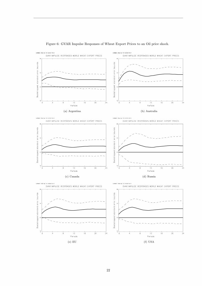
Figure 6: GVAR Impulse Responses of Wheat Export Prices to an Oil price shock.

(a) Argentina (b) Australia

(c) Canada (d) Russia

(e) EU (f) USA

22