A Global Perspective on Railway Inefficiency and the Rise of State Ownership, 1880-1912

Dan Bogart1

Department of Economics UC Irvine

3151 Social Science Plaza A

Irvine CA 92697-5100

Abstract

Railways were one of the important sectors in the early twentieth century and the rise of state ownership was one of the most significant policy changes affecting railways. This paper estimates the inefficiency of railway sectors using stochastic frontier models and a cross-country data set on railway outputs and costs. It also investigates whether inefficiency changed in countries with nationalizations or greater state railway construction. The results show that the trends in inefficiency differed substantially across countries from the 1880s to 1912. The results also show that inefficiency increased with greater nationalizations and decreased with greater state railway construction. Overall the rise of state ownership contributed to lower inefficiency, but the effects depended on whether state ownership increased through nationalizations or new construction. Keywords: Railways; State Ownership; Cost Inefficiency; Stochastic Frontier Estimation;

Globalization

JEL Classifications: N40, N70, L92, P52

1 I would like to thank participants at the International Transport Economics Conference at the University of Minnesota and seminar participants at UC Davis, Kyoto University, UCLA, IMT Lucca, Warwick University, and LSE for comments on earlier versions of this paper. I would also like to thank Jan-Luiten Van Zanden, David Good, Michael Mesch, Max-Stephan Schulze, Roman Studer, Petra Gerlach, Steve Nafziger, Giovanni Federico, and Ola Grytten for providing invaluable help in locating data. Finally I would like to thank Quan Trinh, Sarah Chiu, and Cecilia Lanata Briones for valuable research assistance.

1

1. Introduction

Economic historians often analyze railways through their contribution to social savings.

Contemporaries at the turn of the twentieth century also discussed the developmental effects of

railways, but with equal interest they analyzed the performance of railways as a sector. In 1910

railway revenues equaled around 6% of GDP in countries like Britain and Germany.2 Railway

tracks, locomotives, and stations also constituted a relatively large share of the total capital stock.

According to estimates in the 1880s, railways accounted for around 9% of total wealth in

countries like Britain and Germany (Mulhall 1892, p. 589). Given the large size of the railway

sector and its potential spillover effects on other sectors in the economy, any excess in operating

costs could have substantial implications.

Railway operating expenses differed greatly across countries from the 1880s to 1913 in

part because the scale of outputs (i.e. ton miles and passenger miles), the density of services, and

the price of inputs were all substantially different. However, even after accounting for these

factors, there remain differences in operating expenses both across countries and within

countries. Varying degrees of inefficiency are one reason why expenses differed. In general,

inefficiency arises when firms or organizations do not minimize costs with respect to a given

output level, input price vector, and available technology. In the railway context inefficiency

would be associated with the failure to adopt more energy-efficient locomotives, poor network

design, or the lack coordination across railway lines. Inefficiency would also be associated with

the misallocation of inputs, such as the failure to reduce the use of labor when wages increased

relative to fuel or capital prices. Environmental factors like geography are another explanation

for residual differences in expenses. Variation in elevation or rainfall could contribute to 2 The GDP figures are taken from Mitchell (1992). The sources for revenue will be discussed in the data section.

2

differences in expenses because railways traversed the landscape of a country. Distinguishing

between inefficiency and environmental factors is important because there was scope for

lowering inefficiency through the actions of policy makers, railway managers, and workers.

This paper addresses two questions. How did railway inefficiency differ across countries

from the 1880s to 1912? How did the rise of state ownership influence railway inefficiency

across countries and over time? The rise of state ownership marked one of the major policy

shifts in the railway sector from the 1870s to 1913. Private ownership and operation was

predominant in most countries in 1870. Afterwards there was an evolution towards greater state

ownership and operation through greater construction of state-owned railways and

nationalizations of privately-owned railways. Contemporaries hotly debated the benefits and

costs of state ownership. Some stressed the failings of companies to deliver efficient services

while others pointed to the lack of commercial discipline and the politicization of state railways.3

Today private ownership is generally believed to be more efficient than state ownership

because it encourages competition and arguably provides stronger incentives for investment and

innovation.4 However, it is not obvious that private ownership contributed to efficiency in the

railway context c.1900. Private companies were often guaranteed interest or dividends and thus

had less incentive to cut costs. Moreover it may have been difficult for private companies to

achieve cost savings through the coordination of services.

Although state ownership and operation of railways presented certain advantages,

nationalizations of privately-owned railways arguably raised inefficiency. The transfer price was

often linked to the profits of railway companies over the previous 5 years. Companies

3 For a sample of works see Edwards (1907), Cunningham (1906), Raper (1912), and Dunn (1913). 4 See Shleifer (1998) for summary of recent views on the efficacy of private ownership.

3

anticipating nationalizations had an incentive to cut maintenance expenditures in order to

temporarily boost profits, but once ownership was transferred the added costs of forgone

maintenance set in. More generally the uncertainty surrounding nationalizations may have

encouraged private companies to delay investment or misallocate inputs.

Inefficiency is estimated in this paper using stochastic frontier models and cross-country

data on railway performance. The cross-country data are drawn from a number of sources like

the Statistical Abstract of Foreign Countries, published by the British Board of Trade. It includes

total expenses, railway miles, passenger-miles, ton-miles, and construction costs for railways in

18 of the largest economies. Additional sources were used to combine the railway data with

information on fuel prices and wages in these same economies. The stochastic frontier

methodology involves the estimation of a cost function with the addition of a random term

measuring inefficiency.5 Following other studies, the specification of the cost function includes

variables for scale, density, input prices, and country fixed effects.

The results show that the average level of inefficiency was 0.058, implying the average

country could have reduced its costs by 5.8% in a typical year if it had eliminated all

inefficiency. More significantly the estimates suggest that the trends in inefficiency differed

substantially across countries. The US, Belgium, France, and the Netherlands had the most

efficient railway sectors by the 1900s, while Canada and Italy had the least efficient. In the

1890s the ranking of inefficiencies was quite different. Italy, Sweden, Austria, and Switzerland

had the most efficient railway sectors, while the US and the Netherlands had the least inefficient.

5 For an introduction to stochastic frontier models see Kumbhaker and Lovell (2000).

4

The effects of ownership policies are analyzed using regressions of inefficiency on

variables for the degree of nationalizations, privatizations, and state railway construction. The

results show that inefficiency increased with nationalizations and that inefficiency decreased

with greater state railway construction. By themselves these results do not imply causation, but

they strongly suggest that ownership policies mattered for inefficiency. They also reveal that the

effects of state ownership differed depending on whether there were nationalizations or new state

construction. In countries like Russia, Germany, India, and Italy state ownership tended to

reduce inefficiency because state construction was substantial, but in Switzerland and Japan it

tended to raise inefficiency because they had large nationalizations.

This paper contributes to the historical literature on railway efficiency and productivity. It

builds on the studies by Crafts, Mills, and Mulatu (2007), Crafts, Leunig, and Mulatu (2008),

Leunig (2006), Arnold and McCartney (2005), and Herranz-Loncan (2006), which estimate

freight charges, fares, travel speeds, rates of return, productivity, and inefficiency for British and

Spanish railways before 1912. It also builds on the work of Foreman-Peck (1987) and Bogart

(2009) who analyze construction costs and network development in a cross-country setting.6

The paper also offers a new perspective on the role of policy choices in the global economy

from 1870 to 1913. In this period there was greater government intervention through increased

spending on social services and infrastructure.7 Railways provide an important case to evaluate

the effects of greater government intervention.

6 The paper also relates to the contemporary literature on efficiency estimation. A number of studies have analyzed efficiency at the network or country-level and examined its relationship with ownership or regulatory policies. Some examples include Parisio (1999), Christopoulos, Loizides, and Tsionas (2001), and Cantos and Maudos (2001). 7 See Lindert (2004) and Millward (2004) for studies of social spending and infrastructure.

5

The paper is organized as follows. Section 2 introduces the data. Section 3 displays some

basic patterns in the data. Section 4 discusses the methodology for estimating inefficiency.

Section 5 reports the inefficiency estimates by country and decade. Section 6 analyses the

connection between inefficiency and state ownership. Section 7 concludes.

2. Data

2.1 Railway Performance

Contemporaries collected a substantial amount of data on the financial performance of

railways. Almost every aspect was measured including construction costs, operating expenses,

revenues, and outputs. The British Board of Trade published summary data on railways in

Britain, foreign countries, and British colonies annually starting in the 1870s. The main Board of

Trade publications are the Statistical Abstract for the United Kingdom, the Statistical Abstract

for the Principal and Other Foreign Countries, and the Statistical Abstract for the Several

Colonial and other Possessions of the United Kingdom. These volumes marked one of the first

attempts to compile and present comparable cross-national data. The information is clearly

presented and is easily entered into spreadsheets for statistical analysis.8

The main variables are total railway miles, passengers transported, tons shipped, total

expenses, and construction costs. Railway miles measure the total length of the network.

Passengers transported and tons shipped partly characterize outputs, but they do not incorporate

the distance of the trip or the haul. In some cases the Statistical Abstracts reported the average

haul and the average trip, which along with the data on passengers and tons shipped can be used

8 The statistical Abstracts are now available through web-based versions of the Parliamentary papers. See www. parlipapers.chadwyck.com for details.

6

to calculate passenger miles and ton miles.9 In other cases, International Historical Statistics and

secondary sources provide data on ton miles and passenger miles. The appendix provides full

details on the sources used in each country.

Total expenses measure the operational costs of railways. The data in the Statistical

Abstracts do not distinguish between different types of expenses, so it is not possible to calculate

cost shares. Other data sources show that expenses include the wage bill for train staff and

station staff, spending on fuel, spending on maintenance to the track, plant, and equipment, and

purchases of new capital goods like locomotives.10 The Statistical Abstracts do not report total

expenses for Britain, Australia, India, and Canada; instead they report working expenses, which

are total expenses less spending on new capital goods. In these cases total expenses were

estimated using data from countries that report both working and total expenses.11 The appendix

provides more details.

Construction spending is usually provided separately and is not included in total

expenses. Construction costs were expenses associated with building the track and purchasing

land for the permanent way. Construction costs therefore increased as rail mileage grew, but

they did not necessarily increase at a constant rate because the price of land, materials, and labor

evolved over time.

The financial data on railways needs to be converted into real terms and into a common

currency in order to be comparable across countries and over time. The approach used here is to 9 Passenger miles are calculated by multiplying the number of passengers transported by the average trip in miles; ton miles are calculated by multiplying tons shipped by the average haul in miles. 10 See for example, Estadistica de Los Ferrocarriles en Explotacion for a detailed report on the total expenses of railways in Argentina. 11 Total expenses were estimated using working expenses and the predicted ratio of working to total expenses. The ratio of working to total expenses is fairly constant in most countries and averages 0.94. To improve the estimate the effects of mileage growth were also incorporated. The predicted ratio in year t was estimated to equal 0.94 - 0.0763*(Mileage Growth in year t).

7

first deflate expenses and construction costs in the domestic currency using a domestic consumer

price index with base year 1905 and then convert the figures into 1905 British pounds using the

official exchange rate for 1905.12 Within a particular country the series will represent ‘real’

changes in the expenses of railways. Across countries the series will reflect differences in

expenses valued at the exchange rate. The choice of the 1905 exchange rate matters little

because most countries had a fixed exchange rate during the period under study. Moreover a

different exchange rate for France or any other country will only scale the level of expenses in

France upwards or downwards. In the subsequent efficiency analysis scalar changes in any

variable will be absorbed into the country fixed effects.13

2.2 Input Prices

Different sources are needed to identify the prices of inputs—fuel, labor, and capital.

Coal prices are used to measure the price of fuel because it was the primary source for most

railways. Average coal prices are available for many countries in the Returns Relating to the

Production and Consumption of Coal published by the British Board of trade. The Returns

specify the ‘pit-head’ price of coal in shillings per metric ton for Britain, Russia, Sweden,

Germany, Belgium, France, Spain, Austria, Hungary, Japan, the US, India, Canada, and

Australia. For most years and countries the exchange rate was fixed so the series are effectively

expressed as a domestic coal price series converted at the official exchange rate in 1905. The

12 Consumer Prices indices are generally drawn from Global Financial Database (GFD). The CPI was preferred to the GDP deflator because it is more readily available for the countries studied here. The exchange rates are available in the Statistical Abstracts. See the appendix for details on each country. 13 Another possibility is to use PPP exchange rates. Williamson (1995) provides PPP exchange rates for a sample of countries around 1905. Total expenses for French railways in year t could be converted to PPP adjusted British pounds by multiplying expenses by the formula: (PPP exchange rate pounds per franc 1905) *(CPI UK t)/(CPI France t). A comparison was made between the PPP adjusted total expenditure series and the deflated and converted series used in the analysis for the sample of countries in Williamson. The two series are not identical but they are highly correlated (the correlation coefficient is above 0.99). The reason is that the CPI for the UK is essentially constant for the period from 1883 to 1910 making the two series proportion to one another.

8

coal price series are deflated using the domestic consumer price index for each country to

express coal prices in real terms. The Returns did not cover all countries for which there is

railway data. Information on Dutch, Norwegian, Italian, and Argentine coal prices were taken

from other sources which are described in the appendix.

The earnings of railway employees in the late 1900s are available for the US, UK,

Germany, and Italy in a report by the Bureau of Railway Economics (1912). The report shows

that the average weekly earnings for railway employees were $13.02 for the US, $6.15 for the

UK, $6.25 for Germany, and $5.55 for Italy from 1905 to 1909.14 Williamson’s (1995) data

reports average weekly earnings for skilled and unskilled builders around 1905 in shillings per

week. Converting these earnings into dollars using Williamson’s exchange rate implies that the

average weekly earnings for skilled and unskilled builders were $23.8 and $14.3 for the US, $9.1

and $6.2 for the UK, $6.9 and $5.2 for Germany, $3.4 and $2.1 for Italy (p. 184). With the

exception of Italy, the weekly earnings of the unskilled are very similar to the figures for railway

employees. Building on these data, wages for railway workers are measured using the weekly

wages of unskilled labor in each country (see the appendix for sources).15 The wages are all

deflated using a domestic consumer price index with base year 1905 and then converted to

British shillings using the 1905 official exchange rate.

The user cost of capital is represented by the expression )( δ+rp

p k

, where kp is the price

of capital goods, p is the price of other goods in the economy, r is the interest rate, and δ is the

14 The Bureau of Railway economics used the exchange rate to convert earnings into US dollars. 15 In the later analysis the wages of skilled workers were also included as a robustness check but the results were unaffected.

9

depreciation rate.16 The prices for new capital goods, like locomotives, and materials for repairs

like timber, iron, steel, bricks, etc. are not available for most countries. Fortunately, materials for

repairs to the track and stations were the same or similar as those used for construction of the

track and station. Therefore the construction cost per mile provides a reasonable proxy for the

average price of capital goods. Construction costs are published in the Statistical Abstracts for

most countries. Secondary sources were used for Spain, Italy, and Belgium where construction

costs are not reported (see the appendix for details). The average construction cost per mile was

deflated and converted using the same procedures for wages and coal prices. The interest rate

was assumed to equal the yield on government bonds, which are largely available in Global

Financial Data. The depreciation rate was assumed to be 4% which reflects a 25 year life span

for buildings and locomotives.

2.3 Ownership Variables

The Statistical Abstracts provide information on the number of miles belonging to the

state and the number of miles belonging to companies in each country and year starting in the

1870s. The Report on State Railways, published by the Board of Trade, provides greater details

on ownership and operational practices across countries in 1912. It indicates that private

ownership and operation or state ownership and operation were the dominant forms. Only 3% of

the world’s railway miles were state-owned and privately operated in 1912 and only 1% were

privately owned and state operated.17

The fraction of miles owned by the state provides a simple measure of the extent of state

ownership in a country. It can be misleading though because it masks the sources of state 16 Collins and Williamson (2001) use a similar expression in their study of the user cost of capital . 17 In the sample, the Netherlands, India, and Italy had some state-ownership and private operation. Norway and Austria had some private ownership and state operation.

10

ownership. The number of miles owned by the state can be decomposed into miles initially

owned and constructed by the state plus miles nationalized minus miles privatized.18 These three

variables are used to analyze state ownership because the effects can be different in each case.

Table 1 summarizes the fraction of miles nationalized and constructed by the state in 1880 and

1910 for the sample of countries analyzed here. In 1880 nationalizations were rare outside of a

few countries like Belgium, Germany, India, and Italy. The state constructed a relatively large

proportion of the miles in some countries, including Norway, the Netherlands, Belgium,

Argentina, Germany, and Australia. In others like Britain, Spain, and the US construction of

state-owned railways was absent or negligible.

By 1910 nationalizations had become more common. State-takeovers affected a

relatively large proportion of the miles in Russia, Belgium, Italy, and Germany. The most

extreme cases were Japan, Switzerland, and Austria where over 50% of all miles had been

nationalized by 1910. The degree of state construction also differed across countries by 1910. In

Russia, Germany, Italy, and India the state constructed a greater proportion of the mileage

between 1880 and 1910 and private companies built a lower proportion. In Norway, Japan,

Argentina, Canada, and Australia the opposite trend occurred. The state constructed a smaller

proportion of the mileage, companies a greater proportion. Privatizations were rare in 1880. By

1910 they occurred in Argentina and to a lesser extent in France and the Netherlands.

Other variables are also incorporated as controls. The average elevation, the standard

deviation of elevation, and the skew of elevation can be approximated using data from the Center

for International Earth Science Information Network (CIESIN).19 CIESIN also provides data on

18 See Bogart (2009) for details on the measurement of nationalizations and state ownership. 19 The land area of all countries was normalized to be 100 square meters. The number of square meters within an elevation class was assumed to be equal to the percentage of land in each elevation class. Land was assumed to be

11

the percentage of land area within 100 km of the coast. The number of miles of navigable rivers

and canals is taken from Mulhall (1892, p. 102) and Vernon-Harcourt (1896). The average age

of the network is calculated using the number of miles added in each year as an indicator for the

‘birth’ of track miles. GDP per capita and GDP per capita growth are available from Maddison

(2003) and are expressed in 1990 PPP adjusted US dollars.20 The use of PPP dollars is not crucial

in this context because the GDP figures are correlated with an index of inefficiency.

3. Preliminaries

There were substantial differences in the operating expenses of railways across counties

and over time. Only some of these differences in costs can be explained by variation in scale,

density, and input prices. This section illustrates these points and sets the stage for the

estimation of inefficiency in the following section.

Figure 1 plots the natural log of total operating expenses against the natural log of ton

miles shipped in 1910. Clearly the log of ton-miles explains a substantial portion of the variation

in the log of total expenses. As the graph indicates total expenses are greatest in countries like

the US, Germany, and Russia in large part because they had the greatest ton-miles. However, the

graph also reveals that some countries had similar ton-miles, but total expenses differed.

Consider, for example, that total expenses are lower in India than Canada even though they have

similar ton-miles.

equal to the lower bound in its elevation class to simplify the calculations. Then average, standard deviation, and skew were calculated over the distribution. See Center for International Earth Science Information Network, Columbia University, 2007. National Aggregates of Geospatial Data: Population, Landscape and Climate Estimates, v.2 (PLACE II), Palisades, NY: CIESIN, Columbia University. Available at: http://sedac.ciesin.columbia.edu/place/. 20 GDP data for Russia are taken from Gregory (1982).

12

There are other factors besides ton-miles that can explain differences in operating

expenses across countries. Around 93% of the variation in the natural log of total expenses can

be explained by a pooled OLS regression that includes the log of ton miles, passenger miles, rail

miles, unskilled wages, coal prices, and capital prices as right-hand side variables. Expenses

were higher in countries with higher ton miles and passenger miles. Expenses were higher in

countries with greater wages, coal prices, or capital costs. They were also higher in countries

with a larger rail network all else equal.

Differences in scale, density, and input prices are clearly crucial factors, but they do not

provide a complete characterization of expenses. As an illustration figure 2 plots the residual of

log expenses for Canada and India computed from the pooled regression. Canada’s residual

expenses are initially lower than India, but after the 1900s they rise rapidly. India’s residual

expenses decrease from the 1880s to the 1890s and are significantly below Canada by 1912.

The literature on efficiency estimation characterizes residual operating expenses into two

main types: inefficiency and time-invariant heterogeneity. Inefficiency refers to the added

expenses arising from the failure to adopt best-practice technologies or the misallocation of

inputs. Time-invariant heterogeneity reflects fixed environmental factors which affect costs but

are beyond the control of railway planners, managers, and employees. A goal of the estimation is

to separate inefficiency from time-invariant heterogeneity. It is difficult to fault railway

decision-makers if their geographic environment necessitated extra expenditures on labor, fuel,

and capital. On the other hand they could be faulted if there were added expenses due to the

failure to adopt technologies or misallocate inputs. Current estimation techniques allow the

econometrician to separate inefficiency from all time-invariant heterogeneity by including fixed

effects. Unfortunately, the techniques do not allow the econometrician to estimate inefficiency

13

arising from culture and other institutional factors which do not evolve within the time-span of

the observed data. The following section addresses these issues further and introduces the

econometric methodology.

4. Methodology for Estimating Inefficiency

In the railway context, the translog is the most commonly-used cost function because it

allows for flexible substitution between inputs. It also ‘nests’ the Cobb-Douglas cost function as

a special case. In the main specification the translog cost function will be estimated using the

‘true fixed effects’ model taking the following form:

ititi

K

k

jii

kiikj

J

j

J

l

lii

jiijl

J

j

K

l

lii

kiikl

K

k

J

j

jiij

K

k

kiikit

vuttpq

ppqqpqc

++++++

++++=

∑∑

∑∑∑∑∑∑

==

======

αµµβ

ββββ

221

11

111111

lnln

lnln5.0lnln5.0lnlnln

where itcln is the natural log of real expenses for country i in year t, kitqln is the log of output k

(i.e. ton-miles, passenger-miles, and rail miles) for country i in year t, jitpln is the log of the real

price of input j (i.e. labor, fuel, and capital) for country i in year t, t and 2t are the year and year

squared respectively, iα is a fixed effect for country i, itu is a half-normal random variable with

mean 0 and variance 2uσ , and itv is a normal random variable with mean 0 and variance 2

vσ .

The term itu measures cost inefficiency so that a higher value corresponds with higher costs.

Cost inefficiency is estimated for each country and year using the composite error term

ititit vu +=ε and the parameter estimates for 2uσ and 2

vσ . The conditional mean for cost

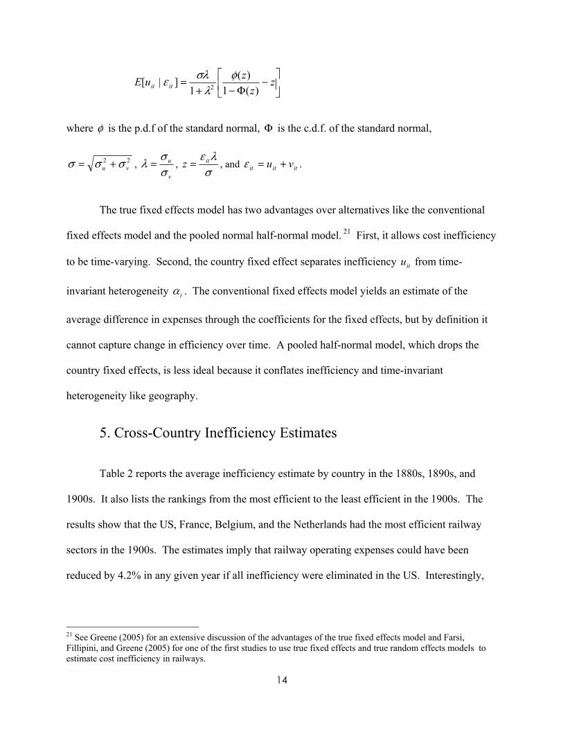
inefficiency is calculated using the following formula from Jondrow et. al. (1982):

14

⎥⎦

⎤⎢⎣

⎡−

Φ−+= z

zzuE itit )(1)(

1]|[ 2

φλ

σλε

where φ is the p.d.f of the standard normal, Φ is the c.d.f. of the standard normal,

22vu σσσ += ,

v

u

σσλ = ,

σλε itz = , and ititit vu +=ε .

The true fixed effects model has two advantages over alternatives like the conventional

fixed effects model and the pooled normal half-normal model. 21 First, it allows cost inefficiency

to be time-varying. Second, the country fixed effect separates inefficiency itu from time-

invariant heterogeneity iα . The conventional fixed effects model yields an estimate of the

average difference in expenses through the coefficients for the fixed effects, but by definition it

cannot capture change in efficiency over time. A pooled half-normal model, which drops the

country fixed effects, is less ideal because it conflates inefficiency and time-invariant

heterogeneity like geography.

5. Cross-Country Inefficiency Estimates

Table 2 reports the average inefficiency estimate by country in the 1880s, 1890s, and

1900s. It also lists the rankings from the most efficient to the least efficient in the 1900s. The

results show that the US, France, Belgium, and the Netherlands had the most efficient railway

sectors in the 1900s. The estimates imply that railway operating expenses could have been

reduced by 4.2% in any given year if all inefficiency were eliminated in the US. Interestingly,

21 See Greene (2005) for an extensive discussion of the advantages of the true fixed effects model and Farsi, Fillipini, and Greene (2005) for one of the first studies to use true fixed effects and true random effects models to estimate cost inefficiency in railways.

15

the US, France, Belgium, and the Netherlands were among the least inefficient in the 1890s. For

the Netherlands this represented a reversal of its earlier status as the most efficient in the 1880s.

There were a large number of countries with ‘medium’ inefficiency in the 1900s. Russia

and Australia had an average inefficiency of 0.051 and 0.052; Britain and India had 0.055 and

0.056; Norway and Spain had 0.057 and 0.058; Argentina and Germany both had an average

inefficiency of 0.059. The trends were varied in this group. Britain, Germany, and Argentina’s

inefficiency increased throughout the period. In India, Norway, and Spain it tended to decrease

over time. India’s efficiency improvements are evident in figure 2 which shows that its residual

costs decreased from the 1880s to the 1890s.

Canada and Italy had the least efficient railway sectors in the 1900s. The estimates

suggest that both countries could have reduced their expenses by at least 7.3% if they eliminated

all inefficiency. Both arrived at this point because their inefficiency increased in the 1900s.

Canada’s rising inefficiency is evident in figure 2 which shows that Canada’s ‘residual’ expenses

were rising in the 1900s. Japan, Switzerland, Austria, and Sweden were slightly more efficient

than Canada and Italy. In all four countries inefficiency increased from the 1890s to the 1900s.

The results also show that the most efficient railway sectors in the 1880s or 1890s were

not necessary the most efficient by the 1900s. The correlation between cost inefficiency in the

1880s and 1890s is negative (see the bottom of table 2). The same is true of the correlation

between cost inefficiency in the 1890s and 1900s. This pattern suggests that greater efficiency

was in many cases replaced by greater inefficiency.

The estimated inefficiency differences across countries are robust to different

specifications. Table 3 reports the summary statistics of inefficiency for alternative

16

specifications like the Cobb-Douglas, the Cobb-Douglas assuming homogeneity of degree one in

input prices, and the translog without country fixed effects.22 It also reports the correlation of the

inefficiency estimates between the translog model with country fixed effects and the rest. The

mean inefficiency estimates are similar between the Cobb-Douglas models and the translog

model with country fixed effects (see columns 1 to 3). More importantly the inefficiency

estimates are highly correlated across these three specifications. This suggests that the estimates

are fairly consistent on which countries had relatively high efficiency and which had relatively

low efficiency.

The inefficiency estimates are different in the translog model without country fixed

effects. Column (4) in table 3 shows that the mean and standard deviation of inefficiency is

higher in this model. Nevertheless there is a reasonably high correlation between the translog

models with and without country fixed effects. Thus inefficiency levels differ in the two models,

but the relative inefficiency differences are similar.

The inefficiency estimates from the translog model without country fixed effects are of

additional interest. They should not be interpreted as inefficiency in a strict sense because they

conflate time-invariant heterogeneity, like geography, with the failure to adopt new technologies

or the misallocation of inputs. Nevertheless they do provide a useful metric for the residual

differences in operating expenses across countries. Table 4 reports the average ‘inefficiency’

estimate by country in the 1880s, 1890s, and 1900s for the translog model without country fixed

effects. The rankings of the countries are generally similar as before. The US, France, and

Belgium still have low inefficiency in the 1900s; Canada and Italy have high inefficiency in the

22 In addition, alternative distributions were tried such as the Gamma and Exponential but the estimates could not be computed. This is not a major concern because most studies find the inefficiency estimates to be similar in the half-normal model compared to the Gamma or Exponential.

17

1900s. The most notable changes are the Netherlands, whose inefficiency is now higher, and

Japan, Switzerland, and Sweden, whose inefficiency is now lower.

The estimates of the cost function are also of interest. Table 5 shows the coefficient

estimates for the translog model with country fixed effects. For comparison, results from the

Cobb-Douglas model are also reported. In the Cobb-Douglas model, the coefficients for ton

miles and passenger miles sum to 0.73, implying economies of scale. The coefficient for rail

miles is 0.3 implying that higher costs result when there is an increase in network size while

holding ton miles and passenger miles constant. The coefficients on the prices for fuel, unskilled

labor, and capital are all positive and significant.

The translog model differs from the Cobb-Douglas because it shows that increases in

input prices have different effects depending on the level of ton miles, passenger miles, and rail

miles. The implication is that the Cobb-Douglas model is too restrictive because the elasticity of

substitution between inputs is not constant. The time trend coefficients in the translog model

suggest that operating costs decreased more rapidly in the 1880s and 1890s than the 1900s. In

1890 costs were 10% lower than in 1882; in 1900 costs were 19% lower than in 1882, and in

1910 they were 22% lower than in 1882. These figures suggest that the railway sector was

experiencing more rapid technological change in the 1880s and 1890s than the 1900s.

Overall the estimates yield a new metric of railway inefficiency across countries and over

time. They suggest that inefficiency was trending upwards in some countries, downward in

others, or some combination. There are a range of factors contributing to the different trends in

inefficiency across countries. The following section focuses on the role of state ownership.

6. State Ownership and Inefficiency

18

State ownership was on the rise from the 1880s to the 1900s. Commentators at the time

consistently pointed to the choice between state or private ownership as being one of the most

important policy decisions facing countries. A number of theories suggest that state or private

ownership can influence inefficiency by altering the incentives of managers, planners, regulators,

and other actors in the industry. The relationship between inefficiency and state ownership is

assessed by a regression of inefficiency in country i and year t on variables measuring the extent

of nationalizations, privatizations, and state railway construction. The first specification includes

control variables for elevation, navigable rivers, the percentage of land area within 100km of the

coast, the average age of the track mileage, GDP per capita, and GDP per capita growth. The

second set of specifications also includes country fixed effects, country specific time trends, and

year fixed effects.

Table 6 shows the results which focus on the cross-country variation. Column (1) reports

estimates from a regression using the broadest measure of state ownership: the fraction of miles

owned by the state. In this specification, and in all others, the inefficiency estimates come from

the baseline translog model summarized in table 2. The results suggest that countries with

greater state ownership did not have significantly higher inefficiency. By itself this finding is

difficult to interpret because state ownership came in various forms. In column (2) state

ownership is decomposed into the fraction of miles nationalized, the fraction constructed by the

state, and the fraction privatized. Column (3) does the same after adding the control variables. In

both specifications nationalizations, privatizations, and greater state railway construction all have

an insignificant relationship with inefficiency.23

23 The results for the control variables are not reported to save space. Only the average age was statistically significant. The coefficient was negative implying that countries with older track mileage were less inefficient.

19

The preceding analysis does not take into account differences in the average level of

inefficiency across countries, differences in the trend of inefficiency across countries, or year

specific shocks to inefficiency. The specifications in table 7 account for these factors by

including country fixed effects, country specific time trends, and year fixed effects into the

regression.24 The results in column (1) show that the effects of ownership are more evident once

these factors are controlled for. There is a positive and significant relationship between

inefficiency and the fraction of miles nationalized, suggesting that inefficiency increased as

nationalizations increased within a country. There is also a negative and significant relationship

between inefficiency and the fraction of miles constructed by the state, suggesting that

inefficiency decreased as state railway construction increased within a country. Lastly, there is

no significant relationship between privatizations and inefficiency.

The same conclusions are suggested by the results in columns (2), (3), and (4). In (2) the

error term in the regression is assumed to be first-order autoregressive and corrects for problems

of serial correlation. The coefficient estimates and their significance are largely unaffected,

except for the privatization variable. In (3) a tobit specification is used to correct the standard

errors for the truncation of the inefficiency index. The coefficient estimates and their

significance are unaffected once again. In (4) the left-hand side variable is replaced by the

inefficiency estimate from the translog model without country fixed effects. Here the estimates

show an even stronger relationship between nationalizations, greater state railway construction,

and inefficiency.25

24 Although the inefficiency estimates are derived from a translog model with country fixed effects, this does not imply that country-specific trends or year specific shocks have been purged from inefficiency. Therefore country fixed effects, country specific time trends, and year fixed effects can still be included in the regression. 25 The results for the control variables are not reported to save space. They show that inefficiency did not increase as a countries’ network aged or if its GDP per capita growth was higher. The results show that increases in GDP per

20

The estimates for the nationalization and state railway construction variables are

generally similar when individual countries are dropped. For example, the estimates are largely

unchanged when India or Italy are dropped. Both had significant state ownership and private

operation. The estimates are also similar when Norway or Austria are dropped. They both had

significant private ownership and state operation. The results are sensitive to the exclusion of one

country: the Netherlands. The Netherlands is an interesting case because its inefficiency varied

significantly over time and therefore its changes in inefficiency are perhaps an outlier. Column

(5) in table 7 shows results after dropping the Netherlands from the estimation. The coefficient

on the nationalization variable drops from 0.109 to 0.069 and the coefficient on state railway

construction decreases in absolute terms from -0.54 to -0.205. Despite their lower magnitude

both variables remain statistically significant.

It is revealing to examine the trends in inefficiency prior to nationalizations and

privatizations. If nationalizations were preceded by greater inefficiency then there might be a

concern that nationalizations were a response to greater inefficiency rather than a contributing

factor. The specifications in table 8 address this issue by relating inefficiency and the fraction

nationalized one, two, or three years before it occurred. The coefficient for the fraction

nationalized one year before is positive and significant. The finding is not surprising because the

process of nationalization often took a year to implement. For example, Japan’s nationalization

was authorized by a law passed in 1906. The assets were transferred from private companies to

the state in 1907 and 1908, which is when the nationalization is dated in the data. If

nationalizations reduced the incentives to invest or maintain railways, then inefficiency should

begin to rise when they were announced, not when the assets were transferred.

capita were associated with higher inefficiency. It is not immediately obvious though why greater income per capita contributed to higher inefficiency. Further study is needed before firm conclusions can be drawn.

21

The results in table 8 also show that inefficiency is insignificantly related to the fraction

nationalized two or three years before. This finding indicates there is no evidence that greater

inefficiency preceded the announcement to nationalize. Figure 3 illustrates this point by plotting

inefficiency 3 years before and 3 years after five major nationalizations: Russia 1894, France

1908, Switzerland 1902, Japan 1907, and Austria 1908. In all cases inefficiency is relatively

stable prior to the year before the nationalization and then rises afterwards.

A similar analysis is conducted for privatizations. The fraction privatized is positive and

significant two or three years before it occurred. This finding indicates that privatizations were

preceded by rising inefficiency and perhaps they were a policy response to inefficiency problems

in the railway sector.

Another issue concerns the long-term effects of nationalizations. Table 9 includes an

interaction between the year and the fraction of miles nationalized to investigate whether the

trend in inefficiency changed after nationalization. The coefficient on the interaction term is

negative and significant, implying that the trend in inefficiency was downward following

nationalizations. Thus the results show that nationalizations initially raised inefficiency but then

inefficiency tended to decrease afterwards. The results in column (2) investigate the timing of the

decline in more detail. The specification includes a variable for the fraction nationalized 3 years

after it occurred. The coefficient is -0.034 suggesting that inefficiency decreased significantly

three years after nationalization.

Together the results point to the conclusion that nationalizations raised inefficiency and

greater construction of state-owned railways reduced inefficiency. Which effect dominated?

Table 10 provides estimates of the net effect of state ownership in each country using the

22

coefficient estimates in column (5) of table 7, the change in the fraction of miles nationalized,

and the change in the fraction of miles constructed by the state between 1890 and 1910 in each

country. The net effect of state ownership was to reduce inefficiency in some countries like

Russia, Germany, India, and Italy. In other countries the net effect of state ownership on

inefficiency was zero or positive. Switzerland and Japan experienced the largest increase in

inefficiency because they had large nationalizations.

The bottom of table 10 reports the weighted average of the net effect of state ownership.

The weights are based on the number of rail miles in each country to give greater importance to

inefficiency changes in countries with larger networks. Across the sample of countries

nationalizations tended to raise inefficiency by 0.003 and state railway construction lowered

inefficiency by 0.005, yielding a net reduction in inefficiency of 0.002. Thus the overall net

effect of state ownership was to lower inefficiency.

7. Conclusion

Railway inefficiency could impose significant costs on economies in the early twentieth

century not only because the railway sector was relatively large, but also because railways had

spillover effects on the rest of the economy. This paper estimates inefficiency using stochastic

frontier models and cross-country data on railway outputs and costs. The results show there were

significant differences in inefficiency across countries and over time. Specifically, the US,

Belgium, France, and the Netherlands had the most efficient railway sectors by the 1900s, but

none of these four countries was in the top ranks of efficiency in the 1890s.

The paper also shows that nationalizations raised inefficiency while greater state railway

construction lowered inefficiency. The results suggest that state ownership per se did not

23

contribute to inefficiency. If that were the case the coefficients on the fraction of miles

nationalized and the fraction of miles built by the state should have been positive, but the latter is

generally negative. Instead the results suggest that large changes in ownership were associated

with increases in inefficiency. This makes sense if private companies stopped maintaining their

track or exerted less effort in monitoring employees once they anticipated nationalizations. It

might also be the case that the transfer of managerial control from the private sector to the

government was generally problematic.

The results also suggest that greater private railway construction c.1900 contributed to

higher inefficiency. Recall that most private railway companies received some type of

guaranteed return on their dividends or bonds. Guarantees were deemed necessary because

private companies were building secondary lines in areas with marginal economic potential.

However, they arguably dulled the incentives for private railways to cut costs. The estimates

also suggest that state railway construction was more efficacious. By the 1890s and 1900s state

bureaucracies were becoming increasingly sophisticated. It appears they were able to resolve the

incentive problems highlighted by their critics at the turn of the century and today.

More broadly the results speak to the effects of policy choices in the period from 1880 to

1912. State intervention in the economy was on the rise in this period. State ownership of

railways provides one of the best examples of this broader phenomenon. The evidence suggests

that this particular case of state intervention was largely beneficial, particularly in countries

where the state built new railways rather than nationalizing private railways.

24

Data Appendix by Country

Russia. The complete data cover the years from 1891 to 1907. The Statistical Abstracts provide

data on railway miles, passengers carried, average journey, tons shipped, average haul, total

expenses, and train miles from 1899 to 1910. Expenses are converted into British pounds using

the official exchange rate of 0.105 pounds for one Rouble in 1905. The 1899 figures for the

average haul and the average journey were assumed to apply for the years 1891 to 1898. Ton

miles and passenger miles are calculated by multiplying tons by the average haul and passengers

by the average journey. Coal prices per metric ton are reported in Returns relating to the

Production, Consumption, etc. of Coal from 1891 to 1907. The prices are reported as average

values in shillings. The official exchange rate was essentially constant (0.10 from 1891 to 1896

and 0.105 from 1897 to 1907) so the reported coal price series is already expressed in shillings at

the 1905 official exchange rate. Weekly wages for unskilled and skilled workers are based on

the real annual earnings of building and railroad staff reported in Allen (2003, p. 38). The series

were converted into weekly nominal earnings using Gregory’s (1982) retail price index and then

converted into British shillings using the 1905 exchange rate. Construction costs per mile were

estimated using Mulhall’s (1892) construction cost figure in 1888 and Gregory (1982) annual

series on railway investment from 1888 to 1907. Gregory’s annual investment series is

converted to 1905 shillings using the exchange rate. Mulhall’s figure for construction is already

expressed in British pounds. All financial variables are deflated using the retail price index from

Gregory (1982) which was converted to the base year 1905. Bond yields come from the Russia

5s of 1822 in London. They are available in GFD which uses the Economist and Banker’s

Magazine (1844-1928).

25

Norway: The complete data cover the years from 1880 to 1912. The Statistical Abstracts

provide data on railway miles, passengers carried, tons shipped, total expenses, train miles, and

construction costs. Expenses and construction costs are converted into British pounds using the

official exchange rate of 0.056 pounds per Kroner in 1905. Ton miles and passenger miles are

taken from Mitchell (1992). Coal prices per metric ton were provided by Ola H Grytten. They

were converted into British pounds using the 1905 official exchange rate. Weekly wages for

unskilled and skilled workers are based on day wages for workers in road construction and

railway staff in Grytten (2007 pp. 281-282, 315-316). The wages are converted into British

shillings using the 1905 exchange rate. All financial variables are all deflated using the

Norwegian consumer price index from Grytten (2004) with base year 1905. Yields are taken

from the 10-year government bond. They are available in GFD and are drawn from The

Economist (1876-1917).

Sweden: The complete data cover the years from 1896 to 1912. The Statistical Abstracts provide

data on railway miles, passengers carried, tons shipped, total expenses, train miles, and

construction costs. Expenses and construction costs are converted into British pounds using the

official exchange rate of 0.056 British pounds per Kronor. Ton miles and passenger miles are

taken from Mitchell (1992). Coal prices per metric ton are reported in Returns relating to the

Production, Consumption, etc. of Coal from 1896 to 1912. The prices are reported as average

values in shillings. The official exchange rate was constant from 1896 to 1912 so the reported

coal price series is already expressed in shillings at the 1905 official exchange rate. Weekly

wages for unskilled and skilled workers are taken from the yearly wages of workers in sawmills

and engineering listed in Bjorklund and Stenlund (1995, p.253). Wages are converted into

shillings using the 1905 exchange rate. All financial variables are deflated using the Swedish

26

consumer price index from Mitchell (1992) with base year 1905. Yields are taken from the 10-

year government bond. They are available in GFD and are drawn from The Economist (1868-

1918).

Netherlands: The complete data cover the years from 1884 to 1902, 1904, 1906, and 1910. The

Statistical Abstracts provide data on railway miles, passengers carried, tons shipped, total

expenses, train miles, and construction costs (state railways only). Expenses and construction

costs are converted into British pounds using the official exchange rate of 0.083 British pounds

per Guilden. Ton miles and passenger miles are taken from Mitchell (1992). Coal prices are

provided by Arthur van Riel through the Global Price and Income History Group

(http://iisg.nl/hpw/data.php#netherlands). The official exchange rate was constant from 1884 to

1910 so the reported coal price series is already expressed in shillings at the 1905 official

exchange rate. The wages for unskilled and skilled workers are based on day wages for laborers

and craftsman in Amsterdam (Allen 2001). The wages of builders are converted into an index

with base year 1905 and multiplied by the weekly earnings of unskilled workers in 1905

shillings, which is estimated using Williamson’s figures for the Netherlands and Britain (1995).

The wages for skilled workers are equal to the weekly wages of unskilled in shillings multiplied

by the ratio of craftsman to builders wages. All financial variables are deflated using the Dutch

consumer price index from Mitchell (1992) with base year 1905. Yields are taken from the 10-

year government bond. They are available in GFD which uses the Economist and Banker’s

Magazine (1844-1928).

Belgium: The complete data cover the years from 1883 to 1910 except 1903 and 1908. The

Statistical Abstracts provide data on railway miles, passengers carried, tons shipped, total

expenses, and construction costs. Expenses and construction costs are converted into British

27

pounds using the official exchange rate of 0.04 British pounds per Belgian Franc in 1905. The

Statistical Abstracts provide the average journey from 1901 to 1912 and the average haul in

1908, 1911, and 1912. The average journey in 1901 was assumed to apply to the period from

1883 to 1900. The average haul in 1908 was assumed to apply for the entire period from 1883 to

1910. Ton miles and passenger miles are then calculated by multiplying tons by the average haul

and passengers by the average journey. The Statistical abstracts provide information on train

miles for all railways from 1901 to 1910 and for state railways from 1883 to 1902. Total train

miles from 1883 to 1900 are assumed to grow at the same annual rate as state railway train miles.

Coal prices per metric ton are reported in Returns relating to the Production, Consumption, etc.

of Coal from 1884 to 1912. The prices are reported as the average value ‘when on the truck for

transportation’ in shillings. The official exchange rate was constant from 1883 to 1912 so the

reported coal price series is already expressed in shillings at the 1905 official exchange rate.

Weekly earnings for unskilled and skilled workers is based on the nominal annual earnings for

manufacturing workers and civil servants in Scholliers (1995, p. 204). The weekly earnings are

converted to shillings using the 1905 exchange rate. All financial variables are deflated using the

Belgian consumer price index from Mitchell (1992) with base year 1905. Yields are taken from

the 10-year government bond. They are available in GFD which uses the Economist and

Banker’s Magazine (1845-1898).

France: The complete data cover the years from 1883 to 1911. The Statistical Abstracts provide

data on railway miles, passengers carried, tons shipped, total expenses, train miles, and

construction costs. Expenses and construction costs are converted into British pounds using the

official exchange rate of 0.04 British pounds per French Franc in 1905. Ton-miles and

passenger-miles are taken from Mitchell (1982). Coal prices per metric ton are reported in

28

Returns relating to the Production, Consumption, etc. of Coal from 1884 to 1912. The prices are

reported as the average value at the pit’s mouth in shillings. The official exchange rate was

constant from 1883 to 1912 so the reported coal price series is already expressed in shillings at

the 1905 official exchange rate. The wages for unskilled and skilled workers are based on the

day wages for laborers and craftsman in Paris (Allen 2001). The wages of builders are converted

into an index with base year 1905 and multiplied by the weekly earnings of unskilled workers in

1905 shillings from Williamson (1995). The wages for skilled workers are equal to the weekly

wages of unskilled in shillings multiplied by the ratio of craftsman to builders’ wages. All

financial variables are deflated using the French consumer price index from Mitchell (1992) with

base year 1905. Yields are taken from the 10-year government bond. They are available in GFD

which uses Investor’s Monthly Manual, London, The Economist (1866-1873), and L’Economiste

Francais (1874-1897).

Switzerland: The complete data cover the years from 1894 to 1912. The Statistical Abstracts

provide data on railway miles, passengers carried, tons shipped, total expenses, train miles, and

construction costs. Expenses and construction costs are converted into British pounds using the

official exchange rate of 0.04 British pounds per Swiss Franc in 1905. Ton miles and passenger

miles are then calculated by multiplying tons by the average haul and passengers by the average

journey. The Statistical abstracts report average haul and the average journey for 1906 to 1912.

The average haul and journey in 1906 was assumed to apply for the whole period from 1894 to

1912. Coal prices are published in Siegenthaler (1996) and were converted to shillings per ton

using the 1905 exchange rate. The wages for unskilled and skilled workers are based on the day

wages for laborers and craftsman (Studer forthcoming). The wages are converted in 1905

shillings per week using the exchange rate. All financial variables are deflated using the Swiss

29

consumer price index from Mitchell (1992) with base year 1905. Yields on government bonds

come from Flandreau and Zumer (2004).

Spain: The complete data cover the years from 1884 to 1909. The Statistical Abstracts provide

data on railway miles, passengers carried, tons shipped, and total expenses. The statistical

abstracts provide data on total expenses from 1898 to 1909. For earlier years total expenses are

estimated from working expenses using the formula discussed in the text. Expenses are

converted into British pounds using the official exchange rate of 0.04 British pounds per Pasetas

in 1905. Ton-miles and passenger-miles are taken from Mitchell (1982). Construction costs per

mile were estimated using Mulhall’s (1892) figure construction costs in 1880 and Herranz-

Locain’s (2005) annual series on railway investment from 1880 to 1909. Herranz’s annual

investment series is converted to 1905 shillings using the exchange rate. Mulhall’s figure for

construction is already expressed in British pounds. Coal prices per metric ton are reported in

Returns relating to the Production, Consumption, etc. of Coal from 1884 to 1912. The prices are

reported as the average value at the pit’s mouth in shillings. The official exchange rate was

constant from 1884 to 1909 so the reported coal price series is already expressed in shillings at

the 1905 official exchange rate. The wages for unskilled and skilled workers are based on the

day wages for laborers and craftsman in Madrid (Allen 2001). The wages of builders are

converted into an index with base year 1905 and multiplied by the weekly earnings of unskilled

workers in 1905 shillings from Williamson (1995). The wages for skilled workers are equal to

the weekly wages of unskilled in shillings multiplied by the ratio of craftsman to builders’

wages. All financial variables are deflated using the Spanish consumer price index from

Flandreau and Zumer (2004) with base year 1905. Yields are taken from the 10-year government

30

bond. They are available in GFD which uses Banker’s Magazine and The Economist (1845-

1910).

Italy: The complete data cover the years from 1890-91, 1898-1901, 1903, 1906, 1911. The

Statistical Abstracts provide data on railway miles, passengers carried, tons shipped, train miles,

and total expenses. Expenses and construction costs are converted into British pounds using the

official exchange rate of 0.04 British pounds per Lire in 1905. Ton-miles and passenger-miles

are taken from Mitchell (1982). Italian coal prices per ton are published in Cianci (1933). They

are converted to British shillings using the 1905 exchange rate. The wages for unskilled and

skilled workers are based on the day wages for construction and engineering (Scholliers and

Zamagni 1995, p. 231). The wages are converted in 1905 shillings per week using the exchange

rate. All financial variables are deflated using the Italian consumer price index from Mitchell

(1992) with base year 1905. Yields are taken from the 10-year government bond. They are

available in GFD which uses The Economist (1863-1914).

Japan: The complete data cover the years from 1894 to 1911. The Statistical Abstracts provide

data on railway miles, passengers carried, tons shipped, total expenses, train miles, and

construction costs. Ton miles and passenger miles are taken from Mitchell (1995). Expenses and

construction costs are converted into British pounds using the official exchange rate of 0.102

British pounds per Yen in 1905. Coal prices per metric ton are reported in Returns relating to the

Production, Consumption, etc. of Coal from 1894 to 1911. The prices are reported as the average

market value in shillings. The exchange rate was essentially constant from 1894 to 1911 (0.105

in 1895 and 1896 and 0.108 in 1897) so the reported coal price series is essentially expressed in

shillings at the 1905 official exchange rate. The wages for unskilled and skilled workers are

based on day wages for laborers and craftsman (masons) in (Allen 2001), which are provided by

31

David Jacks, Peter Lindert, and Salvadore Puente through the Global Price and Income History

Group and are based on the Financial and Economic Annual of Japan. The wages are converted

into shillings per week using the exchange rate in 1905. All financial variables are deflated

using the Japanese consumer price index from Williamson listed in GFD with base year 1905.

Yields are taken from the 10-year government bond. They are available in GFD which uses The

Economist (1870-1914).

US: The complete data cover the years from 1883 to 1911. The Statistical Abstracts provide data

on railway miles, passengers carried, passenger miles, tons shipped, ton miles, total expenses,

train miles, and construction costs. Expenses and construction costs are converted into British

pounds using the official exchange rate of 0.208 British pounds per dollar in 1905. Coal prices

per metric ton are reported in Returns relating to the Production, Consumption, etc. of Coal from

1883 to 1911. The prices are reported as the average spot value in shillings. The exchange rate

was constant from 1883 to 1911 so the reported coal price series is expressed in shillings at the

1905 official exchange rate. The wages for unskilled and skilled workers are based on weekly

earnings for low skilled labor and railway staff (Margo 2006). All financial variables are

deflated using the US consumer price index from U.S. Government, Statistical Abstract of the

United States listed in GFD with base year 1905. Yields are taken from the 10-year government

bond. They are available in GFD which uses the Congressional Budget Office.

Argentina: The complete data cover the years from 1897 to 1912. The Statistical Abstracts

provide data on railway miles, passengers carried, tons shipped, total expenses, train miles, and

construction costs. Expenses and construction costs are converted into British pounds using the

official exchange rate of 0.2 British pounds per peso in 1905. Ton miles, passenger miles, and

average coal prices are taken from Estadistica de Los Ferrocarriles en Explotacion. Coal prices

32

are converted in shillings using the 1905 exchange rate. The wages for unskilled and skilled

workers are based on weekly earnings for railway construction workers and railway staff in

Estadistica de Los Ferrocarriles en Explotacion. All financial variables are deflated using the

Argentina consumer price index from Williamson (1995) with base year 1905. Yields are taken

from the 10-year government bond. They are available in GFD which uses The Economist (1859-

1930).

Britain: The complete data cover the years from 1883 to 1912. The Statistical Abstracts for the

United Kingdom provide data on railway miles, passengers carried, tons shipped, train miles, and

construction costs. Total expenses are estimated from working expenses using the formula

discussed in the text. Ton miles and passenger miles are taken from Crafts, Mills, and Mulatu

(2007). Coal prices per metric ton are reported in Returns relating to the Production,

Consumption, etc. of Coal from 1883 to 1912. The prices are reported as the average value at the

pit’s mouth in shillings. The wages for unskilled and skilled workers are based on the day wages

for laborers and craftsman in London (Allen 2001). The wages of laborers are converted into an

index with base year 1905 and multiplied by the weekly earnings of unskilled workers in 1905

shillings from Williamson (1995). The wages for skilled workers are equal to the weekly wages

of unskilled in shillings multiplied by the ratio of craftsman to builders’ wages. All financial

variables are deflated using the UK consumer price index from Mitchell (1992) with base year

1905. Yields are taken from the 2.5% consol. They are available in GFD which uses Central

Statistical Office, Annual Abstract of Statistics, London: CSO (1853-1912).

Germany: The complete data cover the years from 1883 to 1912. The Statistical Abstracts

provide data on railway miles, passengers carried, passenger miles, tons shipped, ton miles, total

expenses, train miles, and construction costs. Expenses and construction costs are converted into

33

British pounds using the official exchange rate of 0.08 British pounds per mark in 1905. Coal

prices per metric ton are reported in Returns relating to the Production, Consumption, etc. of

Coal from 1883 to 1912. The prices are reported as the average value at the pit’s mouth in

shillings. The official exchange rate was constant from 1883 to 1912 so the reported coal price

series is expressed in shillings at the 1905 official exchange rate. The wages for unskilled and

skilled workers are based on the day wages for laborers and craftsman in Leipzig (Allen 2001).

The wages of laborers are converted into an index with base year 1905 and multiplied by the

weekly earnings of unskilled workers in 1905 shillings from Williamson (1995). All financial

variables are deflated using the German consumer price index from Mitchell (1992) with base

year 1905. Yields are taken from the 10-year bench-mark bond. They are available in GFD

which uses the Bundesbank.

India: The complete data cover the years from 1891 to 1912. The Statistical Abstracts for British

India provide data on railway miles, passengers carried, passenger miles, tons shipped, ton miles,

train miles, and construction costs. Total expenses are estimated from working expenses using

the formula discussed in the text. Expenses and construction costs are converted into British

pounds using the official exchange rate of 0.067 British pounds per rupee in 1905. Coal prices

per metric ton are reported in Returns relating to the Production, Consumption, etc. of Coal from

1883 to 1912. The prices are reported as the average value at the pit’s mouth in shillings using

various exchange rates before 1898 and a constant exchange rate afterwards. Before 1898 Coal

prices are converted back to rupees and then back to shillings using the official exchange rate in

1905. The wages for unskilled and skilled workers are based on the day wages for laborers and

craftsman in five areas Karachi, Beglum, Ahmadgar, Bombay, and Ahmadbad. The wage data

comes from the Statistical Abstract for British India. All financial variables are deflated using

34

the Indian consumer price index from Department of Statistics, Commercial Intelligence

Department listed in GFD with base year 1905. Yields are taken from the 10-year government

bond. They are available in GFD which uses The Economist (1845-1920).

Canada: The complete data cover the years from 1886 to 1912. The Statistical Abstracts provide

data on railway miles, passengers carried, tons shipped, train miles, and construction costs. Total

expenses are estimated from working expenses using the formula discussed in the text. Expenses

and construction costs are converted into British pounds using the official exchange rate of 0.205

British pounds per Canadian dollar in 1905. Coal prices per metric ton are reported in Returns

relating to the Production, Consumption, etc. of Coal from 1886 to 1912. The prices are reported

as the average value in shillings. The official exchange rate was constant from 1886 to 1912 so

the reported coal price series is expressed in shillings at the 1905 official exchange rate. Wage

rates for unskilled and skilled workers are taken from Historical Statistics of Canada and are

converted to British pounds. All financial variables are deflated using the consumer price index

from Minns and MacKinnon (2006) with base year 1905. Yields are taken from the 10-year

government bond. They are available in GFD which uses The Bank of Canada.

Austria: The complete data cover the years from 1894 to 1910. The Statistical Abstracts provide

data on railway miles, passengers carried, tons shipped, train miles, total expenses, and

construction costs. Expenses and construction costs are reported in Gulden before 1900 and are

converted into British pounds using the official exchange rate of 0.083 British pounds per

Gulden. After 1905 expenses and construction costs are reported in Kronen and are converted

into British pounds using the official exchange rate of 0.042 British pounds per Kronen. Ton

miles and passenger miles are taken from Mitchell (1992). Coal prices per metric ton are

reported in Returns relating to the Production, Consumption, etc. of Coal from 1883 to 1912. The

35

prices are reported as the average value at the pit’s mouth in shillings. The prices appear to be

reported using the official exchange rate for Kronen. Weekly wages for unskilled workers are

taken from Mesch (1984). They are converted into British pounds using the exchange rate from

1905. The wages for skilled workers are equal to the weekly wages of unskilled in shillings

multiplied by the ratio of craftsman to builders’ wages in Leipzig drawn from Allen (2001). All

financial variables are deflated using the Austrian consumer price index from Statistical Office,

Statistische Nachrichten listed in GFD with base year 1905. Yields are taken from the 10-year

government bond. They are available in GFD which uses The Economist (1874-1932).

Australia: The complete data cover the years from 1905 to 1912. The Statistical Abstracts

provide data on railway miles, passengers carried, tons shipped, train miles, and construction

costs. Total expenses are estimated from working expenses using the formula discussed in the

text. Expenses and construction costs are expressed in British pounds. Coal prices per metric

ton are reported in Returns relating to the Production, Consumption, etc. of Coal from 1883 to

1912. The prices are reported as the average value at the pit’s mouth in shillings. Wages for

unskilled and skilled workers are taken from the Statistical Abstracts for British Colonies. They

are already expressed in British pounds. All financial variables are deflated using the Australian

consumer price index from the Australian Bureau of Statistics, Digest of Current Economic

Statistics listed in GFD with base year 1905. Yields are taken from the 10-year government

bond. They are available in GFD which uses The Economist (1858-1931).

36

References

Allen, Robert. “The Great Divergence in European Wages and Prices from the Middle Ages to

the First World War.” Explorations in Economic History 38 (2001), pp. 411-447.

Arnold A. and S. McCartney. “Rates of return, concentration levels and strategic change in the

British railway industry 1830-1913.” Journal of Transport History 25 (2005), pp. 41

60.

Bjorklund, Jorgen and Hans Stenlund. “Real Wages in Sweden, 1870-1950: a Study of six

Industrial Branches.” In Scholliers, P. and Zamagni, V., Labour’s Reward: Real Wages

and economic change in 19th and 20th century Europe, New York: Edward Elgar, 1995.

Bogart, Dan. “Nationalizations and the Development of Transport Systems: Cross-Country

Evidence from Railroad Networks: 1860-1912.” Journal of Economic History 69 (March

2009): 202-237.

British Board of Trade, The Statistical Abstract for the Principal and Other Foreign

Countries, Various Years.

British Board of Trade, The Statistical Abstract for the Several Colonial and other Possessions of

the United Kingdom, Various Years.

British Board of Trade, The Statistical Abstract for the United Kingdom, Various Years.

British Board of Trade, Returns Relating to the Production and Consumption of Coal,

Various Years.

British Board of Trade. Report on State Railways: British Possessions and

37

Foreign Countries. London, 1913.

Bureau of Railway Economics. A Comparative Study of Railway Wages and the Cost of Living in The

United States, the United Kingdom, and the Principal Countries of Continental Europe. New

York, 1912.

Cantos, Pedro and Joaquin Maudos, “Regulation and Efficiency: the Case of European

Railways,” Transportation Research Part A 35 (2001): 459-472.

Center for International Earth Science Information Network (CIESIN), Columbia University,

2007. National Aggregates of Geospatial Data: Population, Landscape and Climate

Estimates, v.2 (PLACE II), Palisades, NY: CIESIN, Columbia University. Available at:

http://sedac.ciesin.columbia.edu/place/.

Christopoulos, Dimitris, John Loizides, and Efthymios Tsionas. “Efficiency in European

Railways: Not as inefficient as one might think,” Journal of Applied Economics 4 (May

2001): 63-88.

Cianci, Ernesto. Annali di Statistica series 6 Vol. 20 Rome: ISTAT, 1933.

Collins, William J. and Jeffrey G. Williamson. Capital-Goods Prices and Investment, 1870

1950. Journal of Economic History 61 (March 2001): 59-94.

Crafts, Nicholas, Terence C. Mills, and Abay Mulatu. “Total factor productivity growth on

Britain’s railways, 1852–1912: A reappraisal of the evidence,” Explorations in

Economic History 4 (Oct 2007): 608-634.

Crafts, Nicholas, Timothy Leunig, and Abay Mulatu. “Were British Railway Companies Well

Managed in the early twentieth Century?,” Forthcoming, Economic History Review.

38

Cunningham, William. Should our Railways be Nationalized? London, 1906.

Dunn, Samuel Orace. Government Ownership of Railways. New York, 1913.

Edwards, Clement. Railway Nationalizations. New York, 1907.

Farsi, Mehdi, Massimo Filippini, and William Greene. “Efficiency Measurement in

Network Industries: Application to Swiss Railway Companies,” Journal of Regulatory

Economics 20 (2005): 69-90.

Flandreau, Mark and Frédréric Zumer. The Making of Global Finance, 1880-1913, OECD, 2004.

Foreman-Peck, James. “Natural Monopoly and Railway Policy in the Nineteenth Century.”

Oxford Economic Papers 39 (1987): 699-718.

Greene, William. “Reconsidering Heterogeneity in Panel Data Estimation of the Stochastic

Frontier Model,” Journal of Econometrics 126 (2005): 269-303.

Gregory, Paul. Russian National Income, 1885-1913. Cambridge: Cambridge University Press,

1982.

Grytten, Ola H. “Nominal wages in Norway 1726–1940 by occupation,” in Eitrheim, Øyvind,

Jan T. Klovland and Jan F. Qvigstad (eds.). Historical Monetary Statistics for Norway

Part II. Norges Bank Occasional Papers no. 38, 2007.

Grytten, O.H. "A consumer price index for Norway 1516-2003", 47-98, Historical Monetary

Statistics for Norway 1819-2003, Norges Bank Occasional Papers no. 35, Oslo, 2004.

39

Herranz-Locan, Alfonso. “The Spanish Infrastructure Stock, 1844-1935.” Research in

Economic History 23 (2005): 85-129.

Herranz-Locan, Alfonso. “Railroad Impact in Backward Economies: Spain, 1850-1913.”

Journal of Economic History 66 (Dec. 2006): 853-881.

Jondrow, J., K. Lovell, I. Materov, and P. Schmidt. “On the Estimation of Technical

Inefficiency in the Stochastic Frontier Production Function Model,” Journal of

Econometrics 19 (1982): 233-238.

Kumbhaker, Subal and C.A. Knox Lovell. Stochastic Frontier Analysis. Cambridge:

Cambridge University Press, 2000.

Leacy, F. H. Historical Statistics of Canada. Ottawa, 1983.

Leunig, Tim Leunig, Timothy. "Time is Money: A Re-Assessment of the Passenger Social

Savings from Victorian British Railways," The Journal of Economic History 66 (Sept.

2006): 653-673.

Lindert, Peter. Growing Public: Social Spending and Economic Growth since the Eighteenth

Century. Cambridge, 2004.

MacKinnon, Mary and Chris Minns. “The Costs of Doing Hard Time: A Penitentiary based

Regional Price Index for Canada, 1883-1923,” The Canadian Journal of Economics 40

(May 2007): 528-560.

MacKinnon, Mary. “New Evidence on Canadian Wage Rates, 1900-1930,” The Canadian

Journal of Economics 29 (Feb. 1996): 114-131.

40

Maddison, Angus. The world economy: historical statistics. Paris: Development Centre, OECD,

2003.

Margo, Robert A. , “Hourly and weekly earnings in selected industries and for lower skilled

labor: 1890–1926.” Table Ba4314-4319 in Historical Statistics of the United States,

Earliest Times to the Present: Millennial Edition, edited by Susan B. Carter, Scott

Sigmund Gartner, Michael R. Haines, Alan L. Olmstead, Richard Sutch, and Gavin

Wright. New York: Cambridge University Press, 2006. http://dx.doi.org/10.1017/ISBN

9780511132971.Ba4214-4544

Mesch, Michael. Arbeiterexistenz in der Spatgrunderzeit. Europaverlag Wien, 1984.

Millward, Robert. Private and Public Enterprise in Europe. Cambridge: Cambridge

University Press, 2004.

Minster for Home Affairs, Australia. Year Book of the Commonwealth of Australia, 1910

Mitchell, B.R. International Historical Statistics: Africa, Asia, & Oceania, 1750-1988. New

York: MacMillan, 1995.

Mitchell, B.R. International Historical Statistics: The Americas, 1750-2000. New York:

Palgrave MacMillan, 2003.

Mitchell, B.R. International Historical Statistics: Europe, 1750-1988. New York, MacMillan,

1992.

Mulhall, Michael. Dictionary of Statistics. London: Routledge, 1892.

41

Parisio, Lucia. “A comparative Analysis of European Railway Efficiency: a cost frontier

approach, Applied Economics 31 (1999): 815-823.

Raper, Charles Lee. Railway Transportation: a History of its Economics and its relation to the

State. New York, Knickerbocker Press, 1912.

Republic of Argentina, Ministerio de Obras Publicas. Estadistica de Los Ferrocarriles en

Explotacion, Various Years.

Shleifer, Andre. “State versus Private Ownership,” Journal of Economic Perspectives 12

(Fall 1998).

Scholliers, Peter. “A century of real industrial wages in Belgium, 1840-1939.” In Scholliers, P.

and Zamagni, V., Labour’s Reward: Real Wages and economic change in 19th and 20th

century Europe, New York: Edward Elgar, 1995.

Siegenthaler, Hansjoerg. Historische Statistik der Schweiz Chronos, Zuerich, 1996.

Studer, Roman. “When Did the Swiss Get so Rich? Comparing Living Standards in

Switzerland and Europe,” Forthcoming Journal of European Economic History.

U.S. Department of Commerce. Statistical Abstract of the United States, various years.

Vernon-Harcourt, Leveson Francis. Rivers and Canals. Oxford: Clarendon, 1896.

Williamson Jeffrey G. “The Evolution of Global Labor Markets since 1830: Background

Evidence and Hypotheses,” Explorations in Economic History 32 (April 1995): 141

196.

Table 1: Ownership Patterns across Countries: 1880 and 1910

1880 1910

Country

Fraction

miles nationalized

Fraction miles constructed by

State

Fraction miles

nationalized

Fraction miles constructed by

State

Fraction miles

privatized Russia 0 0.04 0.19 0.44 0.01 Norway 0 0.94 0 0.84 0 Sweden 0 0.33 0.02 0.3 0 Netherlands 0.01 0.57 0.07 0.52 0.04 Belgium 0.24 0.44 0.43 0.5 0.01 France 0.02 0.07 0.12 0.1 0.04 Switzerland 0 0 0.53 0.06 0 Spain 0 0 0 0 0 Italy 0.22 0.22 0.35 0.45 0.01 Japan 0 1 0.55 0.35 0 US 0 0 0 0 0 Argentina 0.01 0.48 0.01 0.24 0.12 Britain 0 0 0 0 0 Germany 0.13 0.51 0.26 0.68 0 India 0.17 0.34 0.22 0.67 0 Canada 0 0.16 0 0.07 0 Austria 0.01 0.07 0.55 0.31 0.03 Australia 0.02 0.92 0.02 0.86 0

Sources: Bogart (2009).

Table 2: Inefficiency Estimates: Baseline Model

Inefficiency

score Efficiency rankings

country 1880-

89 1890-

99 1900-

12 1880-

89 1890-

99 1900-

12 US 0.048 0.087 0.042 5 16 1 France 0.066 0.054 0.044 7 12 2 Belgium 0.062 0.062 0.047 6 15 3 Netherlands 0.026 0.131 0.047 1 17 4 Russia 0.058 0.051 14 5 Australia 0.052 6 Britain 0.045 0.052 0.055 4 10 7 India 0.088 0.044 0.056 9 5 8 Norway 0.07 0.055 0.057 8 13 9 Spain 0.11 0.051 0.058 10 9 10 Argentina 0.048 0.059 8 11 Germany 0.042 0.054 0.059 3 11 12 Japan 0.045 0.065 6 13 Switz. 0.039 0.065 4 14 Austria 0.035 0.071 3 15 Sweden 0.028 0.072 2 16 Italy 0.027 0.073 1 17 Canada 0.042 0.045 0.078 2 7 18 Average 0.06 0.054 0.058 Correlation of inefficiency, 1880s, 1890s -0.54 Correlation of inefficiency, 1890s, 1900s -0.68

Notes: the estimates are based on the translog cost function specification with country fixed effects. Sources: see text.

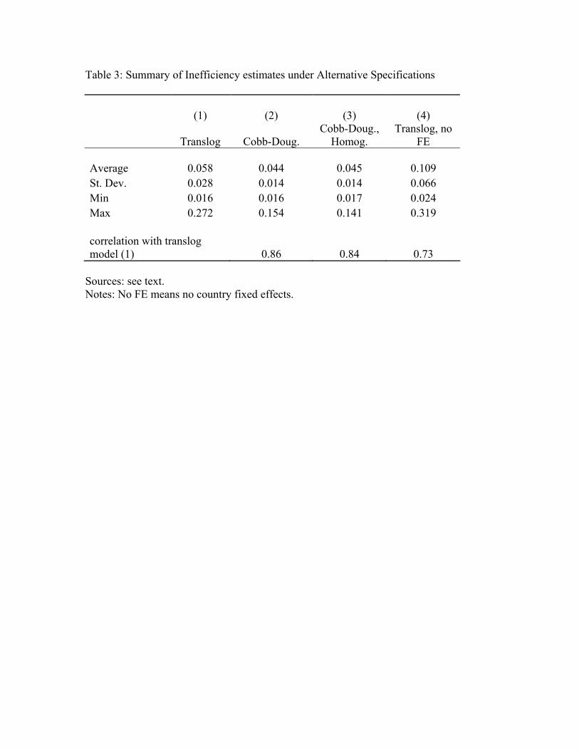
Table 3: Summary of Inefficiency estimates under Alternative Specifications

(1)

Translog

(2)

Cobb-Doug.

(3)

Cobb-Doug., Homog.

(4)

Translog, no FE

Average 0.058 0.044 0.045 0.109 St. Dev. 0.028 0.014 0.014 0.066 Min 0.016 0.016 0.017 0.024 Max 0.272 0.154 0.141 0.319 correlation with translog model (1) 0.86 0.84 0.73

Sources: see text. Notes: No FE means no country fixed effects.

Table 4: Inefficiency Estimates: translog model without country fixed effects

Inefficiency

score Efficiency rankings

country 1880-

89 1890-

99 1900-

12 1880-

89 1890-

99 1900-

12 France 0.062 0.047 0.055 3 3 1 US 0.146 0.143 0.062 9 15 2 Belgium 0.107 0.083 0.066 6 8 3 Japan 0.124 0.086 14 4 Russia 0.095 0.086 10 5 Switz. 0.045 0.095 2 6 Australia 0.097 7 Norway 0.113 0.110 0.099 7 13 8 Argentina 0.098 0.100 11 9 Britain 0.065 0.094 0.114 4 9 10 Sweden 0.053 0.116 4 11 Germany 0.162 0.159 0.142 10 16 12 India 0.089 0.060 0.144 5 7 13 Spain 0.143 0.106 0.147 8 12 14 Canada 0.050 0.060 0.150 1 6 15 Netherland 0.052 0.307 0.160 2 17 16 Austria 0.059 0.160 5 17 Italy 0.042 0.217 1 18 average 0.099 0.099 0.116 Correlation of inefficiency, 1880s, 1890s 0.03 Correlation of inefficiency, 1890s, 1900s 0.07

Notes: the estimates are based on the translog cost function specification without country fixed effects. Sources: see text.

Table 5: Parameter Estimates for the Translog and Cobb-Douglas Cost Functions

Translog Cobb-Douglas Variable Coeff. (Stand. Err.) Coeff. (Stand. Err.) LPM 2.84 (0.85)***

0.33

(0.05)***

LTM -1.60 (0.84)* 0.40 (0.05)*** LRR -0.49 (0.81) 0.30 (0.09)*** LCO -0.62 (0.8) 0.18 (0.05)*** LWA 1.22 (0.77) 0.13 (0.04)*** LCA -4.14 (1.3)*** 0.35 (0.06)*** LPM*LPM -0.10 (0.07) LRR*LRR 0.04 (0.14) LTM*LTM 0.27 (0.11)*** LPM*LTM -0.11 (0.14) LPM*LRR 0.14 (.14) LTM*LRR -0.30 (0.21) LCO*LWA -0.03 (0.09) LCO*LCA -0.03 (0.12) LCO*LCO -0.02 (0.09) LWA*LCA -0.03 (0.12) LWA*LWA 0.03 (0.06) LCA*LCA 0.41 (0.12)*** LPM*LCO -0.08 (0.04)* LPM*LCA 0.02 (0.06) LPM*LWA 0.09 (0.05)* LTM*LCO 0.17 (0.04)*** LTM*LCA -0.13 (0.06)** LTM*LWA -0.06 (0.05) LRR*LCO -0.1 (0.05)* LRR*LCA 0.24 (0.07)*** LRR*LWA -0.16 (0.05)*** YEAR -1.00 (0.33)*** -0.41 (0.36) YEAR*YEAR 0.0002 (0.00008)*** 0.0001 (0.00009) Country fixed effects Yes Yes N 397 397 Log-Likelihood 472 409 Sigma v 0.058 0.077 Sigma u 0.073 0.075

Notes: the dependent variable is the Ln of real total expenses. LCO is the Ln of real coal prices, LCA is the Ln of real capital prices, and LWA is the Ln of real wages. Standard errors are in parentheses. *, **, *** indicates significance at the 10%, 5%, and 1% levels respectively.

Table 6: State Ownership and Inefficiency: Cross-Country Variation

Variable

(1)

Coeff. (Stand. Err.)

(2) Coeff.

(Stand. Err.)

(3) Coeff.

(Stand. Err.) fraction miles owned by state 0.001 (0.003) fraction miles nationalized 0.008 0.019 (0.009) (0.012) fraction miles constructed by state -0.007 -0.002 (0.004) (0.005) fraction miles privatized 0.017 0.032 (0.04) (0.064) Constant 0.057 0.057 0.053 (0.002)*** (0.002)*** (0.012)*** Controls No No Yes country fixed effects No No No N 397 397 397 R-square 0.001 0.02 0.03

Notes: the dependent variable is inefficiency. The control variables include the average elevation, the standard deviation of elevation, the skew of elevation, the % of land area within 100 km of the coast, the number of miles of navigable rivers and canals per square mile, the average age of the track, GDP per capita in the previous year, and the growth rate of GDP per capita. Robust standard errors are in parentheses. *, **, *** indicates significance at the 10%, 5%, and 1% levels respectively.

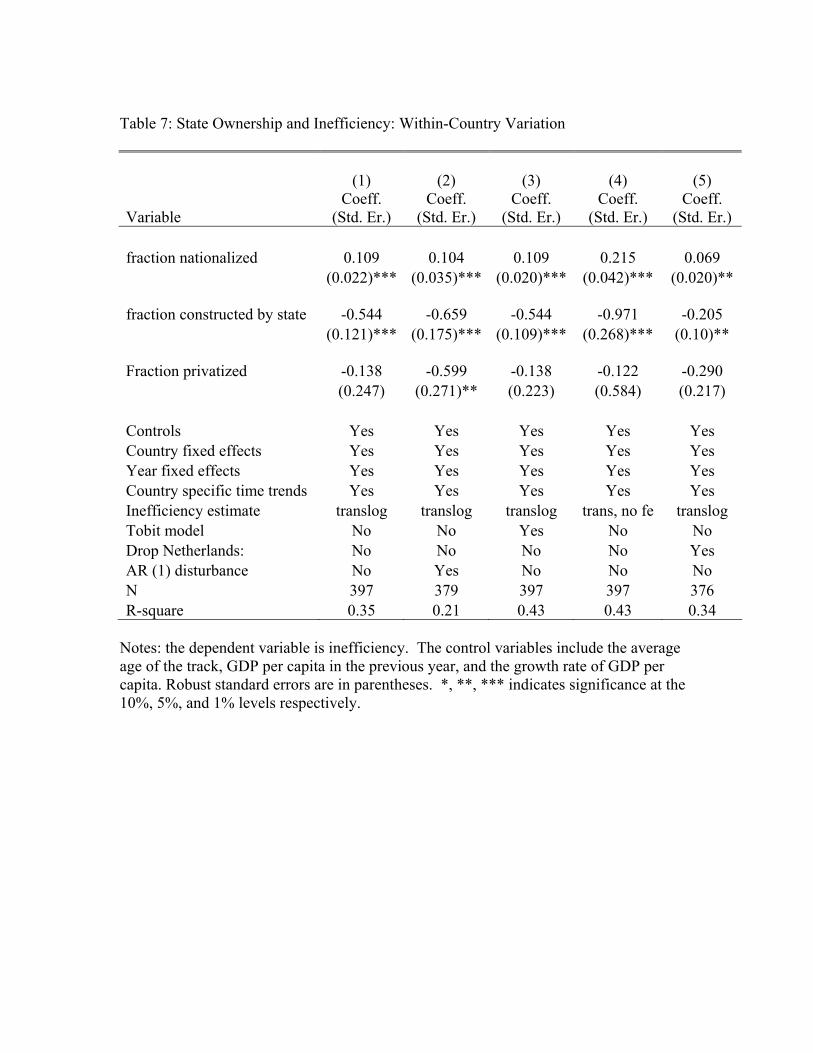
Table 7: State Ownership and Inefficiency: Within-Country Variation

Variable

(1)

Coeff. (Std. Er.)

(2) Coeff.

(Std. Er.)

(3) Coeff.

(Std. Er.)

(4) Coeff.

(Std. Er.)

(5) Coeff.

(Std. Er.) fraction nationalized 0.109 0.104 0.109 0.215 0.069 (0.022)*** (0.035)*** (0.020)*** (0.042)*** (0.020)** fraction constructed by state -0.544 -0.659 -0.544 -0.971 -0.205 (0.121)*** (0.175)*** (0.109)*** (0.268)*** (0.10)** Fraction privatized -0.138 -0.599 -0.138 -0.122 -0.290 (0.247) (0.271)** (0.223) (0.584) (0.217) Controls Yes Yes Yes Yes Yes Country fixed effects Yes Yes Yes Yes Yes Year fixed effects Yes Yes Yes Yes Yes Country specific time trends Yes Yes Yes Yes Yes Inefficiency estimate translog translog translog trans, no fe translog Tobit model No No Yes No No Drop Netherlands: No No No No Yes AR (1) disturbance No Yes No No No N 397 379 397 397 376 R-square 0.35 0.21 0.43 0.43 0.34

Notes: the dependent variable is inefficiency. The control variables include the average age of the track, GDP per capita in the previous year, and the growth rate of GDP per capita. Robust standard errors are in parentheses. *, **, *** indicates significance at the 10%, 5%, and 1% levels respectively.

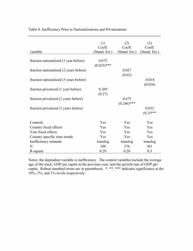
Table 8: Inefficiency Prior to Nationalizations and Privatizations

variable

(1)

Coeff. (Stand. Err.)

(2) Coeff.

(Stand. Err.)

(3) Coeff.

(Stand. Err.) fraction nationalized (1 year before) 0.072 (0.023)*** fraction nationalized (2 years before) 0.027 (0.02) fraction nationalized (3 years before) -0.018 (0.026) fraction privatized (1 year before) 0.269 (0.27) fraction privatized (2 years before) 0.675 (0.246)*** fraction privatized (3 years before) 0.832 (0.3)*** Controls Yes Yes Yes Country fixed effects Yes Yes Yes Year fixed effects Yes Yes Yes Country specific time trends Yes Yes Yes Inefficiency estimate translog translog translog N 388 376 361 R-square 0.29 0.28 0.3

Notes: the dependent variable is inefficiency. The control variables include the average age of the track, GDP per capita in the previous year, and the growth rate of GDP per capita. Robust standard errors are in parentheses. *, **, *** indicates significance at the 10%, 5%, and 1% levels respectively.

Table 9: Trends in Inefficiency After Nationalizations

Variable

(1)

Coeff. (Stand. Err.)

(2) Coeff.

(Stand. Err.) fraction nationalized 24.26 (8.262)** year*fraction nationalized -0.012 (0.004)** fraction nationalized 0.082 (0.021)*** Fraction nationalized (3 years later) -0.034 (0.021) Controls Yes Yes Country fixed effects Yes Yes Year fixed effects Yes Yes Country specific time trends Yes Yes Inefficiency estimate translog translog N 397 397 R-square 0.35 0.3

Notes: the dependent variable is inefficiency. The control variables include the average age of the track, GDP per capita in the previous year, and the growth rate of GDP per capita. Robust standard errors are in parentheses. *, **, *** indicates significance at the 10%, 5%, and 1% levels respectively.

Table 10: Net Effects of the Rise of State Ownership on Inefficiency Country

Effects of nationalizations

Effects of greater state rr construction

Net effect of State Ownership

Russia 0.01 -0.05 -0.04Germany 0 -0.02 -0.02India 0 -0.02 -0.02Italy 0 -0.02 -0.02Netherlands 0 0 0US 0 0 0UK 0 0 0Spain 0 0 0Sweden 0 0 0Austria 0.03 -0.02 0.01Canada 0 0.01 0.01Australia 0 0.01 0.01France 0.01 0 0.01Belgium 0.01 0 0.01Norway 0 0.02 0.02Argentina 0 0.02 0.02Switz. 0.04 -0.01 0.03Japan 0.04 0.03 0.07 Weighted average 0.003 -0.005 -0.002

Notes: Estimates use the change in the fraction nationalized and the fraction constructed by the state in each country from 1890 to 1910 and the coefficient estimates from Table 7 column 5.

Figure 1: Scatter Plot of Log Ton Miles vs. Log Total Expenses, 1910

Rus

Nor

SweNet

Bel

Fra

Swi Spa

Itl

Jap

US

Arg

GbrGer

IndCanAust

Ausl

13.5

14.5

15.5

16.5

17.5

18.5

19.5

20.5

18 19 20 21 22 23 24 25 26

Log Ton Miles

Log

Tota

l Exp

ense

s

Figure 2: Residual Total Expenses in India and Canada, 1887-1912

-0.35

-0.3

-0.25

-0.2

-0.15

-0.1

-0.05

0

0.05

0.1

0.15

1887 1889 1891 1893 1895 1897 1899 1901 1903 1905 1907 1909 1911

can india

Figure 3: Three years before and after 5 Major Nationalizations

0

0.02

0.04

0.06

0.08

0.1

0.12

0.14

-3 -2 -1 0 1 2 3

Year (0=Nationalization)

Inef

ficie

ncy

Russia 1894 france 1908 switzerland 1902 Japan 1907 Austria 1908