A Geometric Method for Analyzing of Second-Order ... · A Geometric Method for Analyzing of...

A Geometric Method for Analyzing of Second-Order Autonomous Systems and Its Applications

HASSAN FATHABADI

Post-Doc researcher Engineering Department

Kharazmi University Tehran, IRAN

[email protected]

NIKOS E. MASTORAKIS Industrial Engineering Department

Technical University of Sofia Sofia 1000, BULGARIA

[email protected] Abstract: - In this paper, the behavior of a second-order dynamical system around its equilibrium point will be analyzed based on the behavior of some appropriate equipotential curves which will be considered around the same equilibrium point. In fact two sets of equipotential curves are considered so that a set of the equipotential curves has a role as the upper band of the system trajectory and another set plays a role as the lower band. It will be shown that stability of the system around its equilibrium point can be assessed using the behavior of these two set of equipotential curves. As will be shown, asymptotically stability and instability analysis of the system only need the analysis of the upper band set of the equipotential curves, but oscillation behavior analysis of the system need to analyze both the lower band set of the equipotential curves and the upper band set. The method can even detect a stable limit cycle appearing in the oscillation systems. The proposed method is geometric and has some applications such as designing of oscillators. Finally, some examples, practical designing of oscillators and simulation results will be presented to verify and validate the presented method. Key-Words: - Equilibrium point, stability, instability, autonomous system. 1 Introduction

As we know, two classic methods are essentially used to analyze the stability of a nonlinear system [1], [2]. The first method is stability analysis using energy function and the second method is based on the linearization of the system around its equilibrium point. Sometimes the first method is called “Direct Method” and the second method is called “Indirect Method”. In fact, the first method was presented by the mathematician called Lyapunov. The complexity of the first method is to find the appropriate energy functions to assess the stability of a nonlinear system. The second method has two major weaknesses. Firstly, if the eiginvalues of the coefficient

matrix in the linear system resulted of linearization have real parts that are equal zero, the original nonlinear system may be stable or instable around the equilibrium point. Secondly, the method can only assess stability as the form of local stability around the equilibrium point. The proposed method mentioned in this paper is a geometric method which is suitable to analyze the stability of a second-order autonomous systems. This kind of system is very important because it models the behavior of some devices such as oscillators [3].

Also two basic methods are essentially used to analyze the behavior of limit cycles appearing in nonlinear system [1], [2]. The first method is to draw the trajectories of the system using the softwares such as Matlab in order to

WSEAS TRANSACTIONS on SYSTEMS Hassan Fathabadi, Nikos E. Mastorakis

E-ISSN: 2224-2678 106 Issue 3, Volume 11, March 2012

mailto:[email protected]

mailto:[email protected]

detect the limit cycles of the system. It is clear that the limit cycles that is detected by this approach can be recognized as stable, unstable or semi-stable [1], [2]. The second method is based on the linearization of the system around its equilibrium point or points. The second method has two major weaknesses. Firstly, the equilibrium point of the system, which the system is linearized around it, must be on the limit cycle or in a small neighborhood of it otherwise the method can not detect the real behavior of the nonlinear system. Secondly, the method can only assess the behavior of the system around the limit cycle as the form of point to point if and only if these points all locate on the limit cycle [1]. Also there are several classic methods to design oscillators. The most general and important method is based on using the equation, which the open loop transfer function of the system or electronic circuit equals minus one [3]. It is clear that the design is done in Laplace domain. As we will see, the proposed geometric method in this paper is much easier than above method to design electronic oscillator [3], [4]. There are some researches presenting some geometric and numerical methods to analyze the stability and behavior of some special systems such as Josephson junction system [5-19]. These methods can not be applied for analyzing of general second or higher order systems. 2 Equipotential Curves

Consider the second-order autonomous system described by the following equation

⎪⎩

⎪⎨⎧

=

=

)2,1(22

)2,1(11xxfx

xxfx

&

& (1)

Definition 1: A set is said “compact” if it is

bounded and closed [1], [4]. Definition 2: Consider the set called so that P

2RP ⊂ , P is said “invariant set” if the trajectories of the system beginning in the P remain in it as [1], [20], [21]. ∞→t

Definition 3: Suppose that the is the equilibrium point of the second-order autonomous system described by the equation (1) and suppose that the compact set called M

includes the equilibrium point (the origin). The closed curves belonging the M, which is described by o that

0=X

Cxxu =)2,1( s RC∈ and

enclosing the equilibrium point, are called equipotential curves because for each value of

there is a closed curve with the potential of , so all points locating on the

CC Cxxu =)2,1(

have the equal potential the numerical quantity of which is C .

3 Stability Analysis

Theorem 1: The second-order autonomous system described by (1) is local asymptotic stable around the equilibrium point ( 0=X ) if there are equipotential curves Cxxu =)2,1(

with clockwise direction, enclosing the equilibrium point and further on the trajectories of the system (1)

)2,1(

dt

xxdu0< . (2)

Proof: From , we have Cxxu =)2,1(

0*)2,1(

*)2,1(

22

11

=∂

∂+

∂

∂x

x

xxux

x

xxu&& (3)

and as a result, the dynamic of Cxxu =)2,1(

can be expressed as

⎪⎪

⎩

⎪⎪

⎨

⎧

∂

∂−=

∂

∂=

1

2

)2,1(2*

)2,1(1*

x

xxux

x

xxux

&

&

(4)

where and are the state variables of the

dynamic of . The velocity vector

on the

1*x& 2*x&

Cxxu =)2,1(

Cxxu =)2,1( symbolized by uVr

is

define as 21 2*1* xxu uxuxV r

&r

&r

+= , so from (4)

we found that

21)

)2,1((

)2,1(

12xxu u

x

xxuu

x

xxuV rrr

∂

∂−+

∂

∂= (5)

where 1xur and

2xur are respectively the unity vectors of the axis and axis. Also, the

velocity vector of the system (1) is defined as 1x 2x



21 21 xx uxuxX r

&r

&r& += ,so it can be written as

21)2,1(2)2,1(1 xx uxxfuxxfX rrr

& += . (6)

The derivative dt

xxdu )2,1( on the trajectories of

the system (1) can be expressed as

22

11

)2,1()2,1()2,1(x

x

xxux

x

xxu

dt

xxdu&&

∂

∂+

∂

∂= (7)

or

XV

xxfx

xxuxxf

x

xxu

dt

xxdu

u

r&

r×=

∂

∂+

∂

∂= )2,1(2

)2,1()2,1(1

)2,1()2,1(

21 (8)

where )sin(. αXVXV uu

r&

rr&

r=× and α is the angle

between and uVr

Xr& . So the inequality (2) can be

written as

0<× XVu

r&

r (9)

and this means that the direction of the trajectories of the system (1) are to inside of the equipotential curves as shown in

Fig. 1, on the other hand and C can be changed so that closed curves

Cxxu =)2,1(

RC∈Cxxu =)2( ,1

enclosing the equilibrium point could tend to be smaller and smaller and finally approach to the equilibrium point (the origin). This means that the direction of the trajectory of the system (1) will tend to the origin, so the system (1) is asymptotically stable.

Theorem 2: The second-order autonomous system described by (1) is unstable around the equilibrium point ( 0=X ) if there are equipotential curves with

clockwise direction, enclosing the equilibrium point and further on the trajectories of the system (1)

Cxxu =)2,1(

0)2,1(>

dt

xxdu. (10)

Proof: It follows from the proof of the theorem 1 that inequality (10) means that

0>× XVu

r&

r (11)

and in the similar manner with the proof of the theorem 1, the direction of the trajectories of the system (1) are to outside of the equipotential curves Cxxu =)2,1( as shown in Fig. 2, so the

trajectories tend to infinity ( far and farther of the equilibrium point) and this means that the system around the equilibrium point ( 0=X ) is unstable.

Definition 4: A limit cycle is said asymptotic stable if all trajectories in vicinity of the limit cycle converge to it as . Otherwise the limit is semi-stable or unstable[2].

∞→t

Theorem3: Consider the second-order autonomous system (1), suppose that no equilibrium point belongs to the compact set M which encloses the origin ( ). There are equipotential curves and

0=X1211 ),( Cxxu =

2212 ),( Cxxu = with clockwise directions that belong to M, does not intersect one with another, enclose the origin and satisfy the following inequalities on the trajectories of the system (1)

0),( 211 ≥dt

xxdu (12)

0),( 212 ≤dt

xxdu (13)

if and only if there exists an asymptotic stable limit cycle L so that

Ω⊂ intL (14) where )21,( CCΩ is the region located between

1211 ),( Cxxu = and . 2212 ),( Cxxu =

Fig. 1.The system is asymptotic stable.



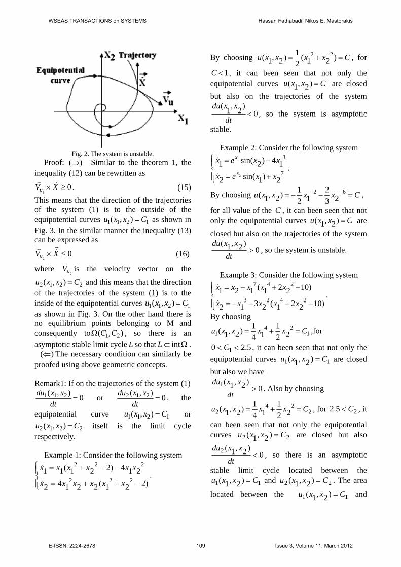
Fig. 2. The system is unstable.

Proof: Similar to the theorem 1, the inequality (12) can be rewritten as

)(⇒

01

≥× XVu

r&

r. (15)

This means that the direction of the trajectories of the system (1) is to the outside of the equipotential curves as shown in Fig. 3. In the similar manner the inequality (13) can be expressed as

1211 ),( Cxxu =

02

≤× XVu

r&

r (16)

where is the velocity vector on the

and this means that the direction of the trajectories of the system (1) is to the inside of the equipotential curves

2uVr

2212 ),( Cxxu =

1211 ),( Cxxu = as shown in Fig. 3. On the other hand there is no equilibrium points belonging to M and consequently to , so there is an asymptotic stable limit cycle

),( 21 CCΩL so that Ω⊂ intL .

)(⇐ The necessary condition can similarly be proofed using above geometric concepts. Remark1: If on the trajectories of the system (1)

0),( 211 =dt

xxdu or 0),( 212 =dt

xxdu , the

equipotential curve or itself is the limit cycle

respectively.

1211 ),( Cxxu =

2212 ),( Cxxu =

Example 1: Consider the following system

⎪⎩

⎪⎨⎧

−++=

−−+=

)221(22142

214)221(11222

222

xxxxxx

xxxxxx

&

&.

By choosing Cxxxxu =+= )21(21)2,1( 22 , for

1<C , it can been seen that not only the equipotential curves are closed but also on the trajectories of the system

Cxxu =)2,1(

0)2,1(<

dt

xxdu, so the system is asymptotic

stable. Example 2: Consider the following system

⎪⎩

⎪⎨⎧

+=

−=7

3

2)1sin(2

14)2sin(12

1

xxex

xxexx

x

&

&.

By choosing Cxxxxu =−−= −− 6223

212

1)2,1( ,

for all value of the , it can been seen that not only the equipotential curves

CCxxu =)2,1( are

closed but also on the trajectories of the system

0)2,1(>

dtxxdu

, so the system is unstable.


⎪⎩

⎪⎨⎧

−+−−=

−+−=

)10221(2312

)10221(1212423

247

xxxxx

xxxxx

&

&.

By choosing

124

1 221

141)2,1( Cxxxxu =+= ,for

5.20 1 << C , it can been seen that not only the equipotential curves are closed but also we have

11 )2,1( Cxxu =

0)2,1(1 >

dtxxdu

. Also by choosing

224

2 221

141)2,1( Cxxxxu =+= , for 25.2 C< , it

can been seen that not only the equipotential curves 22 )2,1( Cxxu = are closed but also

0)2,1(2 <

dtxxdu

, so there is an asymptotic

stable limit cycle located between the 11 )2,1( Cxxu = and . The area

located between the 22 )2,1( Cxxu =

11 )2,1( Cxxu = and



22 )2,1( Cxxu = is an invariant set as the following

⎭⎬⎫

⎩⎨⎧ <+<=Ω 2

24121 22

114

1)2,1(),( CxxCxxCC (17)

where . It is clear that the limit cycle can be estimated by varying the

and in (17). In above set by increasing and decreasing , the limit cycle can be

found as

21 5.20 CC <<<

1C 2C

1C 2C

5.2221

141 24 =+ xx .

4 Control of Limit Cycle Using State

Feedback Consider the following nonlinear

autonomous system

⎪⎩

⎪⎨⎧

=

=

),,(

),,(*22122

*12111

uxxfx

uxxfx

&

& (18)

where and are the control inputs as the form of state feedback presented by the following equations

*1u *

2u

⎪⎩

⎪⎨⎧

=

=

),(

),(

212*2

211*1

xxhu

xxhu. (19)

Now, the question is that how and must be chosen so that an asymptotic

stable limit cycle can be added to the system

(18)? The condition

),( 211 xxh),( 212 xxh

0),( 211 ≥dt

xxdu on the

trajectories of the system (18) in the theorem 3 can be rewritten as following inequality

0),,(),(

),,(),(

*2212

2

211

*1211

1

211

≥

+

uxxfdx

xxdu

uxxfdx

xxdu

(20)

and in the similar manner the 0),( 212 ≤dt

xxdu

appeared in the theorem 3, can be expressed as

0),,(),(

),,(),(

*2212

2

212

*1211

1

212

≤

+

uxxfdx

xxdu

uxxfdx

xxdu

. (21)

The inequalities (20) and (21) give the conditions which have to be satisfied by ,

, and in order to appear an asymptotic limit cycle in the system (18).

*1u

*2u ),( 211 xxu ),( 212 xxu


⎪⎩

⎪⎨⎧

+−−=

+−=*22

2112

*1

31

721

uxxxx

uxxx

&

& (22)

It is clear that the equilibrium point at the origin is asymptotic stable. Now, the state feedback lows ( and ) have to be determined so that an asymptotic stable limit cycle can be added to the resulted closed loop system. By choosing equipotential curves as

*1u *

2u

18

22

1211 4),( Cxxxxu =+= ; (23) 120 1 <<C

28

22

1212 4),( Cxxxxu =+= ; (24)

214 C<

and replacing (23) and (24) in (20) and (21), respectively the following inequalities are found

0)(8)(8 *22

211

72

*1

31

721 ≥+−−++− uxxxxuxxx ;

for (25) 1240 82

21 <+< xx

and 0)(8)(8 *

222

117

2*1

31

721 ≤+−−++− uxxxxuxxx ;

for . (26) 82

21414 xx +<

It can be derived from (25) and (26) that 08888 *

27

2*11

82

21

41 ≥++−− uxuxxxx ;

for (27) 1240 82

21 <+< xx

and 08888 *

27

2*11

82

21

41 ≤++−− uxuxxxx ;

for . (28) 82

21414 xx +<

By choosing the state feedback laws as the following forms

⎪⎩

⎪⎨

⎧

==

+==

0),(

)43(),(

212*2

821211

*1

xxhu

xxxxhu β (29)



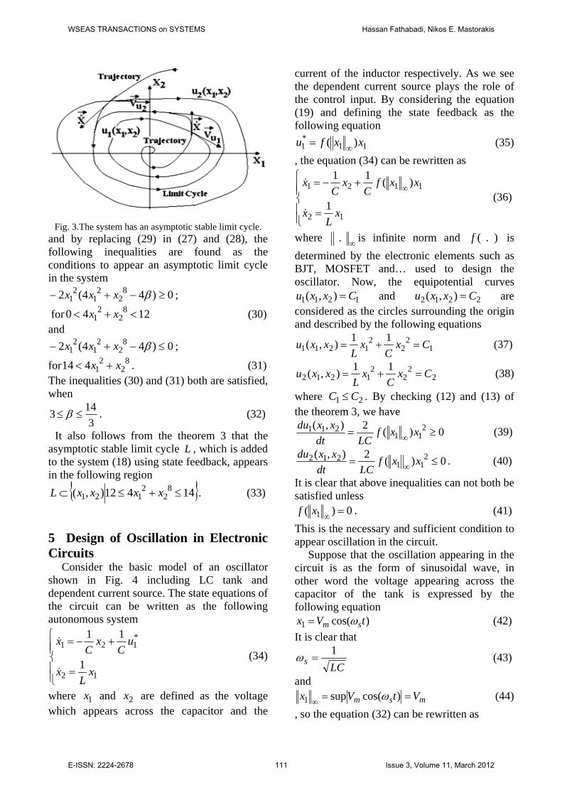
Fig. 3.The system has an asymptotic stable limit cycle. and by replacing (29) in (27) and (28), the following inequalities are found as the conditions to appear an asymptotic limit cycle in the system

0)44(2 82

21

21 ≥−+− βxxx ;

for (30) 1240 82

21 <+< xx

and 0)44(2 8

22

12

1 ≤−+− βxxx ;

for . (31) 82

21414 xx +<

The inequalities (30) and (31) both are satisfied, when

3143 ≤≤ β . (32)

It also follows from the theorem 3 that the asymptotic stable limit cycle L , which is added to the system (18) using state feedback, appears in the following region

{ }14412),( 82

2121 ≤+≤⊂ xxxxL . (33)

5 Design of Oscillation in Electronic Circuits

Consider the basic model of an oscillator shown in Fig. 4 including LC tank and dependent current source. The state equations of the circuit can be written as the following autonomous system

⎪⎪⎩

⎪⎪⎨

⎧

=

+−=

12

*121

1

11

xL

x

uC

xC

x

&

&

(34)

where and are defined as the voltage which appears across the capacitor and the

current of the inductor respectively. As we see the dependent current source plays the role of the control input. By considering the equation (19) and defining the state feedback as the following equation

1x 2x

11*1 )( xxfu ∞= (35)

, the equation (34) can be rewritten as

⎪⎪⎩

⎪⎪⎨

⎧

=

+−= ∞

12

1121

1

)(11

xL

x

xxfC

xC

x

&

&

(36)

where ∞. is infinite norm and is determined by the electronic elements such as BJT, MOSFET and… used to design the oscillator. Now, the equipotential curves

).(f

1211 ),( Cxxu = and are considered as the circles surrounding the origin and described by the following equations

2212 ),( Cxxu =

12

22

121111),( CxC

xL

xxu =+= (37)

22

22

121211),( CxC

xL

xxu =+= (38)

where 21 CC ≤ . By checking (12) and (13) of the theorem 3, we have

0)(2),( 211

211 ≥= ∞ xxfLCdt

xxdu (39)

0)(2),( 211

212 ≤= ∞ xxfLCdt

xxdu . (40)

It is clear that above inequalities can not both be satisfied unless

0)( 1 =∞xf . (41) This is the necessary and sufficient condition to appear oscillation in the circuit.

Suppose that the oscillation appearing in the circuit is as the form of sinusoidal wave, in other word the voltage appearing across the capacitor of the tank is expressed by the following equation

)cos(1 tVx sm ω= (42) It is clear that

LCs1

=ω (43)

and msm VtVx ==∞ )cos(sup1 ω (44)

, so the equation (32) can be rewritten as



0)()( 1 ==∞ mVfxf . (45)

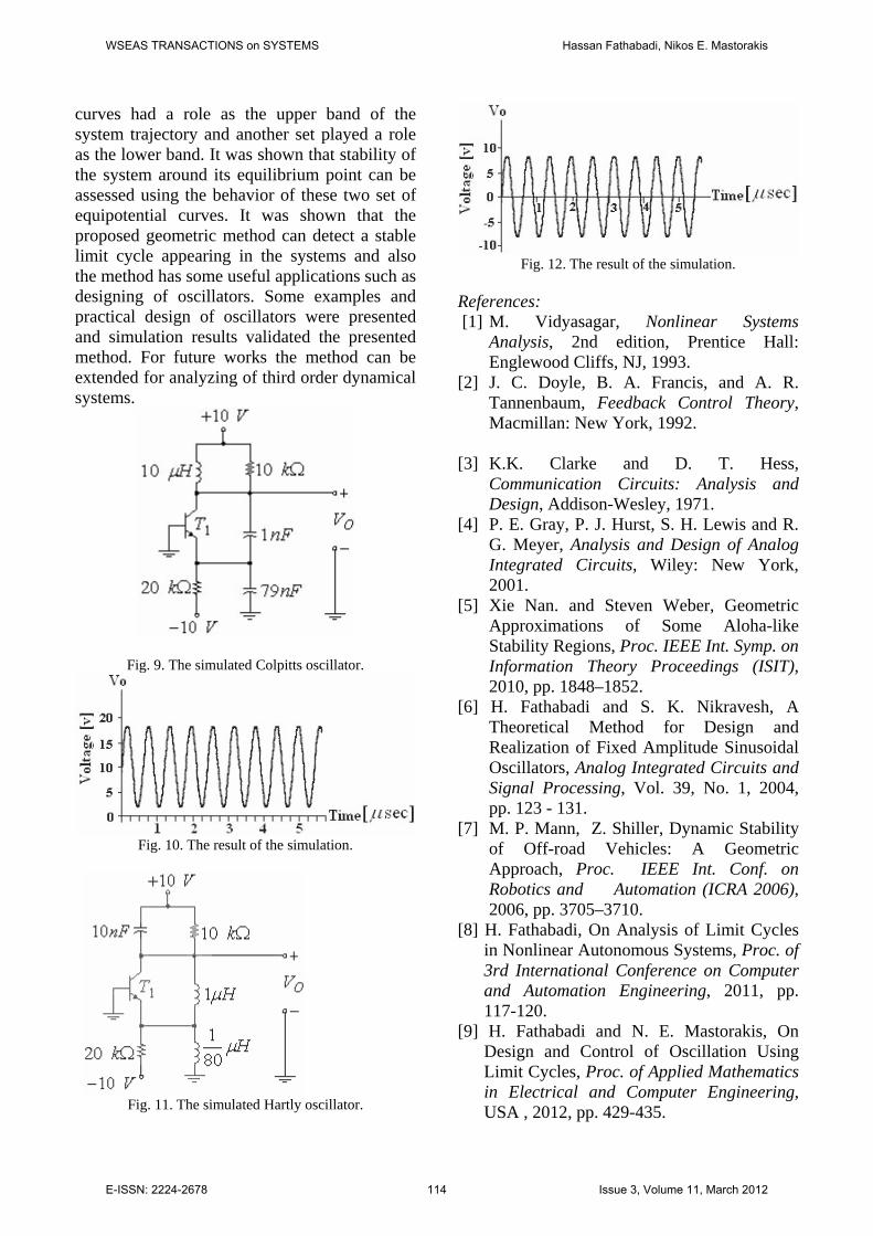
Example 5: Consider the Hartly and Colpitts

oscillators shown in Fig. 5 and Fig. 6 and their equivalent circuit shown in Fig. 7. The equivalent circuit can be summarized and drawn again as Fig. 8. By comparing Fig. 8 and Fig. 4 and using equation (45), the necessary and sufficient condition to appear sinusoidal oscillation on the output of the Hartly and Colpitts oscillators can be found as the following equation

0))(()()( 2 =+−−=α

mmELmmm

nVGGnGnnVGVf

where is the large signal transconductance of the BJT used in the oscillator. It derives from the above equation that

).(mG

)1()(

2

αnn

GnGnVG ELmm

−

+= . (46)

From equation (46), the necessary and sufficient condition to appear oscillation in the Colpitts oscillator can be rewritten as

)1(

)( 2

αnng

GnGgnVG

m

EL

m

mm

−

+= (47)

where is the small signal transconductance of the BJT evaluated at the quiescent point. By

defining

mg

)( qkTnVx m= where

KJk 231037.1 −×=

is boltzmann constant and is the charge of an electron, the equation (47) can be rewritten as

Cq 19106.1 −×=

)1(

)( 2

αnng

GnGg

xG

m

EL

m

m

−

+= . (48)

On the other hand, we have [3]

])(

))(ln(1[)()(2)( 0

0

1

kTqV

xIxxIxI

gxG

m

m

λ+= , (49)

where is the sum of the quiescent voltages appearing across the total resistance between

base and emitter and is a modified Bessel function of order n and is defined as

λV

)(xIn

∫+

−=

π

πθ θθ

πdnexI x

n )cos(21)( cos . (50)

It can be derived from equations (48) and (49) that

)1(]

)(

))(ln(1[)()(2 2

0

0

1

αλ nng

GnG

kTqV

xIxxIxI

m

EL

−

+=+ . (51)

The equation (51) can be used to earn the amplitude of the oscillation ( ). mV

Example 6: Consider the Colpitts oscillator

shown in Fig. 9 so that , ,

, , ,

and

Ω= kRL 10 nFC 11 =

nFC 792 = Ω= kRE 20 HL μ10=

VVCC 10−= 199.0 ≈=α .

We have

nFCC

CCC 121

21 ≈+

= ,801

21

1 =+

=CC

Cn ,

and VV 3.9=λ mAk

VII EC 465.0

20

3.9=

Ω=≈ .

The frequency can be found as

Fig. 4. The basic model of an oscillator.

Fig. 5. The Hartly oscillator.



Fig. 6. The Colpitts oscillator.

Fig. 7. The equivalent circuit of the oscillators.

Fig. 8. The summarized equivalent circuit of the

oscillators.

sec101 7 radLCs ==ω

and

1

561 −Ω==

kTqIg C

m .

Replacing , , , mg n LG α and EG in equation (44) results that

448.0])026.0

3.9())(ln(1[

)()(2 0

0

1 =+xI

xxIxI (52)

We obtain and the numerical solution

of the equation (52) and replacing in

5.3≈x

)( qkTnVx m=

gives , and finally VVm 9.7=

][)10cos(9.710)( 7 vttVO += . (53) The circuit was simulated by PROTEUS-6

software and again repeated by PSPICE-8

software, the results were the same. As we see, the result of the simulations shown in Fig. 10, validates the proposed geometric method and the numerical result expressed by eq. (54).

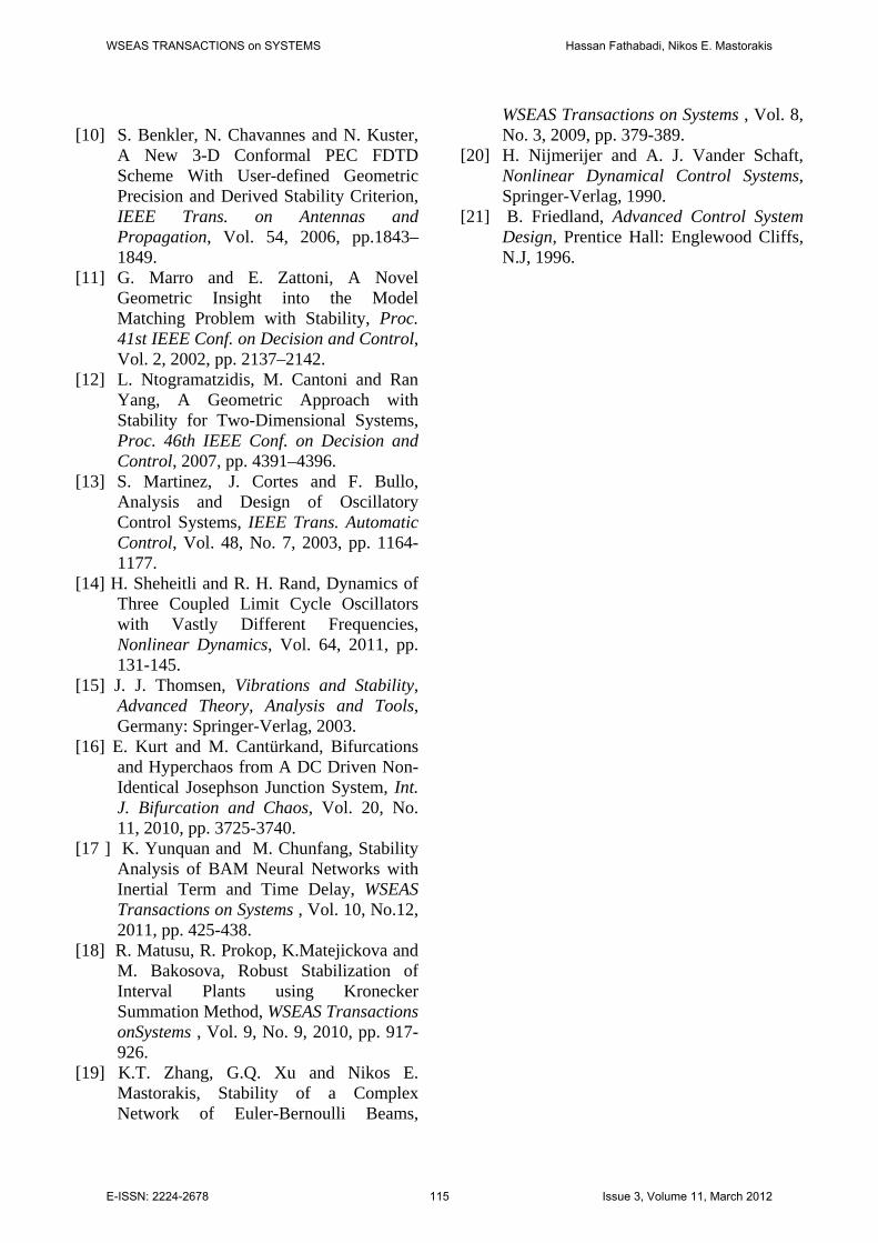
Example 7: Consider the Hartly oscillator

shown in Fig. 11 so that ,

, ,

Ω= kRL 10

nFC 10= Ω= kRE 20 HL μ11 = ,

HL μ801

2 = , and VVCC 10−= 199.0 ≈=α .

We have

HLLL μ121 ≈+= ,801

21

2 ≈+

=LL

Ln ,

and VV 3.9=λ mAk

VII EC 465.0

20

3.9=

Ω=≈ .

The frequency can be earn as

sec101 7 radLCs ==ω

and

1

561 −Ω==

kTqIg C

m .

Replacing , , , mg n LG α and EG in equation (51) results that

448.0])026.0

3.9())(ln(1[

)()(2 0

0

1 =+xI

xxIxI (54)

Again we obtain 5.3≈x and the numerical solution of the equation (46) and replacing in

)( qkTnVx m= results that . So we

have

VVm 9.7=

][)10cos(9.7)( 7 vttVO = . (55) Again the simulation result shown in Fig. 12 validates the proposed geometric method and the numerical result expressed by eq. (55).

6 Conclusion

In this paper, the behavior of a second-order dynamical system around its equilibrium point was analyzed based on the behavior of some appropriate equipotential curves which were considered around the same equilibrium point. In fact two sets of equipotential curves were considered so that a set of the equipotential



curves had a role as the upper band of the system trajectory and another set played a role as the lower band. It was shown that stability of the system around its equilibrium point can be assessed using the behavior of these two set of equipotential curves. It was shown that the proposed geometric method can detect a stable limit cycle appearing in the systems and also the method has some useful applications such as designing of oscillators. Some examples and practical design of oscillators were presented and simulation results validated the presented method. For future works the method can be extended for analyzing of third order dynamical systems.

Fig. 9. The simulated Colpitts oscillator.

Fig. 10. The result of the simulation.

Fig. 11. The simulated Hartly oscillator.

Fig. 12. The result of the simulation.

References: [1] M. Vidyasagar, Nonlinear Systems

Analysis, 2nd edition, Prentice Hall: Englewood Cliffs, NJ, 1993.

[2] J. C. Doyle, B. A. Francis, and A. R. Tannenbaum, Feedback Control Theory, Macmillan: New York, 1992.

[3] K.K. Clarke and D. T. Hess,

Communication Circuits: Analysis and Design, Addison-Wesley, 1971.

[4] P. E. Gray, P. J. Hurst, S. H. Lewis and R. G. Meyer, Analysis and Design of Analog Integrated Circuits, Wiley: New York, 2001.

[5] Xie Nan. and Steven Weber, Geometric Approximations of Some Aloha-like

Regions, Proc. IEEE Int. Symp. on Information Theory Proceedings Stability

(ISIT), 2010, pp. 1848–1852.

[6] H. Fathabadi and S. K. Nikravesh, A Theoretical Method for Design and Realization of Fixed Amplitude Sinusoidal Oscillators, Analog Integrated Circuits and Signal Processing, Vol. 39, No. 1, 2004, pp. 123 - 131.

[7] M. P. Mann, Z. Shiller, Dynamic of Off-road Vehicles: A Approach, Proc.

StabilityGeometric

IEEE Int. Conf. on Robotics and Automation (ICRA 2006), 2006, pp. 3705–3710.

[8] H. Fathabadi, On Analysis of Limit Cycles in Nonlinear Autonomous Systems, Proc. of 3rd International Conference on Computer and Automation Engineering, 2011, pp. 117-120.

[9] H. Fathabadi and N. E. Mastorakis, On Design and Control of Oscillation Using Limit Cycles, Proc. of Applied Mathematics in Electrical and Computer Engineering, USA , 2012, pp. 429-435.



http://ieeexplore.ieee.org/search/srchabstract.jsp?tp=&arnumber=5513425&queryText%3Dstability+geometric%26openedRefinements%3D*%26searchField%3DSearch+All







[10] S. Benkler, N. Chavannes and N. Kuster,

A New 3-D Conformal PEC FDTD Scheme With User-defined Precision and Derived Criterion, IEEE Trans. on Antenna

GeometricStability

s and Propagation, Vol. 54, 2006, pp.1843–1849.

[11] G. Marro and E. Zattoni, A Novel Insight into the Model

Matching Problem with Geometric

Stability, Proc. 41st IEEE Conf. on Decision and Control, Vol. 2, 2002, pp. 2137–2142.

[12] L. Ntogramatzidis, M. Cantoni and Ran Yang, A Approach with

for Two-Dimensional Systems, Geometric

StabilityProc. 46th IEEE Conf. on Decision and Control, 2007, pp. 4391–4396.

[13] S. Martinez, J. Cortes and F. Bullo, Analysis and Design of Oscillatory Control Systems, IEEE Trans. Automatic Control, Vol. 48, No. 7, 2003, pp. 1164-1177.

[14] H. Sheheitli and R. H. Rand, Dynamics of Three Coupled Limit Cycle Oscillators with Vastly Different Frequencies, Nonlinear Dynamics, Vol. 64, 2011, pp. 131-145.

[15] J. J. Thomsen, Vibrations and Stability, Advanced Theory, Analysis and Tools, Germany: Springer-Verlag, 2003.

[16] E. Kurt and M. Cantürkand, Bifurcations and Hyperchaos from A DC Driven Non-Identical Josephson Junction System, Int. J. Bifurcation and Chaos, Vol. 20, No. 11, 2010, pp. 3725-3740.

[17 ] K. Yunquan and M. Chunfang, Stability Analysis of BAM Neural Networks with Inertial Term and Time Delay, WSEAS Transactions on Systems , Vol. 10, No.12, 2011, pp. 425-438.

[18] R. Matusu, R. Prokop, K.Matejickova and M. Bakosova, Robust Stabilization of Interval Plants using Kronecker Summation Method, WSEAS Transactions onSystems , Vol. 9, No. 9, 2010, pp. 917-926.

[19] K.T. Zhang, G.Q. Xu and Nikos E. Mastorakis, Stability of a Complex Network of Euler-Bernoulli Beams,

WSEAS Transactions on Systems , Vol. 8, No. 3, 2009, pp. 379-389.

[20] H. Nijmerijer and A. J. Vander Schaft, Nonlinear Dynamical Control Systems, Springer-Verlag, 1990.

[21] B. Friedland, Advanced Control System Design, Prentice Hall: Englewood Cliffs, N.J, 1996.












A Geometric Method for Analyzing of Second-Order ... · A Geometric Method for Analyzing of...

Documents

Transcript of A Geometric Method for Analyzing of Second-Order ... · A Geometric Method for Analyzing of...