
A Geometric Look At Repeated Measures Design with Missing...
11
Pertanika 7(2), 71-81 (1984) A Geometric Look At Repeated Measures Design with Missing Observations AHMAD BIN ALWI and C.]. MONLEZUN 1 Department of Mathematics, Universiti Pertanian Malaysia Serdang, Selangor, Malaysia. Key words: Repeated measures design; subspaces; noncentrality parameters; orthogonal: orthonormal basis. RINGKASAN Di dalam kertas ini kami akan memberi gambaran geometri bagi Rekabentuk Sukatan Berulang untuk bilangan subjek yang tak sama serawatan yang mempunyai kehilangan cerapan. Untuk pembentukan geometri, kami menghadkan rekabentuk ini kepada tiga tahap bagi fakt01' A dan empat tahap bagi faktor B. Tujuan kertas ini ialah untuk membentuk ujian statistik bagi hipotesis yang dikehendaki iaitu tiada kesan utama A, tiada kesan utama B, dan tiada tindakan bersaling AB. SUMMARY In this paper, we will provide a geometric view of Repeated Measures Design for unequal number of subjects per treatment that has missing observations. For our geometric development we restrict our design to three levels of factor A and four levels of factor B. The purpose of this paper is to develop a test statistics for hypotheses of interest i.e. no main effect A, no main effect B, and no AB interaction. 1. INTRODUCTION The data for a two-factor Repeated Design is collected and tabulated in a data table as shown in Figure 1. Let Y.. be the measurement made on subject i at level j of factor A and level k of factor B. For illustrative purposes, we let , b=4, n 1 =3, n 2 =2, n 3 =4. B 1 B 2 B 3 B 4 Yll1 Yl12 Y 113 Y114 Al Y 211 Y212 Y213 Y 214 Y 311 Y312 Y 313 Y 314 A 2 Y121 Y 122 Y123 Y124 Y221 Y222 Y 223 Y224 Y131 Y132 Y133 Y 134 A 3 Y231 Y 232 Y 233 Y234 Y331 Y 332 Y 333 Y 334 Y 431 Y 432 Y433 Y434 Figure 1: Data table for observations. We arbitrarily set the observations Y Y 113' 312' Y123 , Y 232' Y 233 and Y 334 as missing. We model our experiment as: Yijk = U jk + S.. + E" k (1.1 ) IJ IJ 1 Assoc. Professor, Dept. of Experimental Statistics, Louisiana State University, U.S. A Key to author's name: A. Ahmad. 71
Transcript of A Geometric Look At Repeated Measures Design with Missing...

Pertanika 7(2), 71-81 (1984)
A Geometric Look At Repeated Measures Design with MissingObservations
AHMAD BIN ALWI and C.]. MONLEZUN1
Department ofMathematics,Universiti Pertanian MalaysiaSerdang, Selangor, Malaysia.
Key words: Repeated measures design; subspaces; noncentrality parameters; orthogonal: orthonormalbasis.
RINGKASAN
Di dalam kertas ini kami akan memberi gambaran geometri bagi Rekabentuk Sukatan Berulanguntuk bilangan subjek yang tak sama serawatan yang mempunyai kehilangan cerapan. Untuk pembentukangeometri, kami menghadkan rekabentuk ini kepada tiga tahap bagi fakt01' A dan empat tahap bagi faktorB. Tujuan kertas ini ialah untuk membentuk ujian statistik bagi hipotesis yang dikehendaki iaitu tiadakesan utama A, tiada kesan utama B, dan tiada tindakan bersaling AB.
SUMMARY
In this paper, we will provide a geometric view of Repeated Measures Design for unequal numberof subjects per treatment that has missing observations. For our geometric development we restrict ourdesign to three levels of factor A and four levels of factor B. The purpose of this paper is to develop a teststatistics for hypotheses of interest i.e. no main effect A, no main effect B, and no AB interaction.
1. INTRODUCTION
The data for a two-factor Repeated Measu~es
Design is collected and tabulated in a datatable as shown in Figure 1. Let Y.. be themeasurement made on subject i (1S:i'S::~~ at levelj (1~j~a) of factor A and level k (1~k'S:b) offactor B. For illustrative purposes, we let a=~ ,b=4, n
1=3, n
2=2, n
3=4.
B1
B2
B3
B4
Yll1 Yl12 Y 113 Y114
Al Y211 Y212 Y213 Y 214
Y 311 Y312 Y 313 Y314
A2
Y121 Y122 Y123 Y124
Y221 Y222 Y223 Y224
Y131 Y132 Y133 Y134
A3
Y231 Y232 Y233 Y234
Y331 Y332 Y333 Y334
Y431 Y432 Y433 Y434
Figure 1 : Data table for observations.
We arbitrarily set the observations Y Y113' 312'
Y123 , Y232' Y233 and Y334 as missing. We modelour experiment as:
Yijk = Ujk + S.. + E" k (1.1 )IJ IJ
1 Assoc. Professor, Dept. of Experimental Statistics, Louisiana State University, U.S. A
Key to author's name: A. Ahmad.
71
AHMAD BIN ALWI AND c.r. MONLEZUN
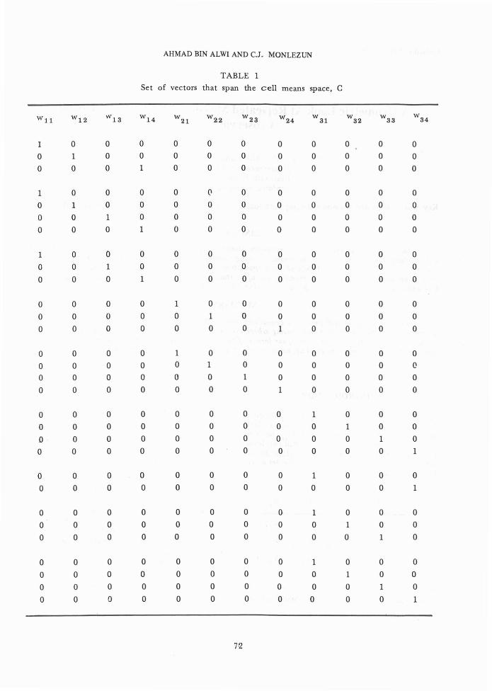
TABLE 1
Set of vectors that span the cell means space, C
w I1 w 12w
13 w 14 w w 22w
23 w 24 w 31 W32
W33
W3421
1 0 0 0 0 0 0 0 0 0 0 0
0 1 0 0 0 0 0 0 0 0 0 0
0 0 0 1 0 0 0 0 0 0 0 0
1 0 0 0 0 (\ 0 0 0 0 0 0
0 1 0 0 0 0 0 0 0 0 0 0
0 0 1 0 0 0 0 0 0 0 0 0
0 0 0 1 0 0 0 0 0 0 0 0
1 0 0 0 0 0 0 0 0 0 0 0
0 0 1 0 0 0 0 0 0 0 0 0
0 0 0 1 0 0 0 0 0 0 0 0
0 0 0 0 1 0 0 0 0 0 0 0
0 0 0 0 0 1 0 0 0 0 0 0
0 0 0 0 0 0 0 1 0 0 0 0
0 0 0 0 1 0 0 0 0 0 0 0
0 0 0 0 0 1 0 0 0 0 0 0
0 0 0 0 0 0 1 0 0 0 0 0
0 0 0 0 0 0 0 1 0 0 0 0
0 0 0 0 0 0 0 0 1 0 0 0
0 0 0 0 0 0 0 0 0 1 0 0
0 0 0 0 0 0 0 0 0 0 1 0
0 0 0 0 0 0 0 0 0 0 0 1
0 0 0 0 0 0 0 0 1 0 0 0
0 0 0 0 0 0 0 0 0 0 0 1
0 0 0 0 0 0 0 0 1 0 0 0
0 0 0 0 0 0 0 0 0 1 0 0
0 0 0 0 0 0 0 0 0 0 1 0
0 0 0 0 0 0 0 0 1 0 0 0
0 0 0 0 0 0 0 0 0 1 0 0
0 0 0 0 0 0 0 0 0 0 1 0
0 0 a 0 0 0 0 0 0 0 0 1
72

A GEOMETRIC LOOK AT REPEATED MEASURES DESIGN WITH MISSING OBSERVATIONS
2. GEOMETRIC DEVELOPMENT
where { S.. , E" k } are 9+30 = 39 mutually11 IJ
independent normal random variables each havingmean zero, with Var(Sij) = a~, Var(Eijk) =ai.AlternatIvely we can write the model as
A = span { aI' a2 } ,
B = span { b1, b2 , b 3 } ,
AB = span {(ab)11' (ab)12' (ab)13. (ab)21' (abk'
(ab )23 } ,
'Within subject space" , Ws = span { s11' s21'
s31' s12' s22' s13' s23' 53 3' s43} where Sij'S
are defined in Table 4, and
We now define subspaces of R30 which facilitatethe construction of test statistics. Let
(1.2)
i1=i' or jt=j'
i=i' andj=j' and kt=k'
Yijk is N( V jk , a: + a~
and
The observational vector is written as:
Y. Y.. , Y"2' Y'3' Y" 4 ]' for ij=21.22,13,43IJ IJl IJ IJ IJ
,Y11 = Y111 , Y112 , Yl14 ]
Y12 = Y121 , Y122 , Y124 ]'
Y23 = Y231' Y 234]'
Y31 = Y311' Y313' Y314] ,
Y33 = Y331' Y332' Y333] ,
l' = Ws I±l B ffJ AB.
T is the smallest subspace contammg both Cand Ws' We defined the Error space, E, asthe space orthogonal both to C and Ws i.e.E = span { e1 , e2 ,... , e12 } where e's are definedin Table 5.
3. HYPOTHESES TESTING
The hypotheses of interest are:
V. = V.,J. )
V. k = V k'
[' , , Fly' •
Y = Y 11' Y 21' Y 31' Y i2' Y 22' 13' Y 23'
1 '] ,
Y 33' Y 43
Y is a vector in the Euclidean space withdimension 30, R30.
In general, when there are missing observationsfor subjects an exact test of H A is not available.
Why not have an exact test for H A?
The cell means vector is written as:3 4
E(Y) = k k V' k w' k where w' k is defined mj=lk=l)) J
Table 1
The set of w'k vectors form a basis for the cellmeans space,) C, having dimension 12. If weparameterized V jk = U + aj + b k ·+ (ab)jk
subjected to the conditions
~ aj =f bk = T (ab)jk = f (ab)ik = 0
theA the cell means space, C, has a basis theset of vectors { 130 , a1 , a2 , b1 , b2 , b g , (ab)ll'
(ab)12' (ab)13' (ab)21' (ab)22' (ab)23 } as
defined in Table 2.
Var(Y) = ail + a~J where I is the n .. x n..identity matrix and J is a matrix defined inTable 3.
The hypothesis for no main effect A in V jk is
H A : Vi. = Vi'.
<::::=> aj = 0 <==> KA' u = 0 <==> G)~~(Y)
:::: 0 <==> E(Y) C WA = 130
ffJ B I±l AB (3.1)
( KA , V, and GA ~re defined as in Table 6).
To assure a central F distribution when H A istrue, we need the numerator space for calculatingSum of squares for A, NA' to be orthogonal toWA •
If we want NA' to be orthogonal to Ws also we
would define NA = l' g [ B I±l AB I±l Ws ].
But T = [ B I±l AB I±l Ws ], therefore, NA
{ } and we do not have test statistics. Ifwe want NA -L Ws (as in the case when all observations on a subject are present), note that
73

AHMAD BIN ALWI AND c.J. MONLEZUN
TABLE 2
After reparamaterization, alternative basis for C
130 ~,a2 b 1 b 2 b 3 (ab)11 (ab )12 (ab )13 (ab)21 (ab)22 (ab)23
1 1 0 1 0 0 1 0 0 0 0 0
1 1 0 0 1 0 0 1 0 0 0 0
1 1 0 -1 -1 -1 -1 -1 -1 0 0 0
1 1 0 1 0 0 1 0 0 0 0 0
1 1 0 0 1 0 0 1 0 0 0 0
1 1 0 0 0 1 0 0 1 0 0 0
1 1 0 -1 -1 -1 -1 -1 -1 0 0 0
1 1 0 1 0 0 1 0 0 0 0 0
1 1 0 0 0 1 0 0 1 0 0 0
1 1 0 -1 -1 -1 -1 -1 -1 0 0 0
1 0 1 1 0 0 0 0 0 1 0 0
1 a 1 0 1 a a a 0 a 1 a1 a 1 -1 -1 -1 a a a -1 -1 -1
1 a 1 1 a a a a a 1 a a1 a 1 a 1 a a a a a 1 0
1 a 1 a a 1 a a a a a 1
1 a 1 -1 -1 -1 a a a -1 -1 -1
1 -1 -1 1 a a -1 a a -1 a 0
1 -1 -1 0 1 a 0 -1 a a -1 a1 -1 -1 a a 1 a a -1 a 0 -1
1 -1 -1 -1 -1 -1 1 1 1 1 1 1
1 -1 -1 1 a a -1 a 0 -1 0 0] -1 -1 -1 -1 -1 1 1 1 1 1 1
1 -1 -1 1 a a -1 a a -1 a a1 -1 -1 0 1 a a -1 a a -1 a1 -1 -1 0 0 1 a a -1 a a -1
1 -1 -1 1 0 a -1 a a -1 0 a1 -1 -1 '0 1 a a -1 a a -1 a1 -1 -1 0 0 1 a a -1 a a -11 -1 -1 -1 -1 -1 1 1 1 1 1 1
74

A GEOMETRIC LOOK AT REPEATED MEASURES DESIGN WITH MISSING OBSERVATIONS
TABLE 3
J Matrix
111
1 1 11 1 1
o 0 0 0
o 0 0 0
o 0 0 0
000
000
000
000
o 0 0
000
o 000
o 0 0 0
o 0 0 0
o 0 0 0
o 0 0 0
o 0 0 0
o 0 000
o 0 0 0 0
o 0 000
000 0
000 0
000 0
000
000
000o 0 0
1 1 1 11 1 1 1
1 1 1 1111 1
000
000
000
000
o 0 0
o 0 0
000
000
00000000
00000000
00000000
00000000
o 0 0 0 0
o 0 0 0 0
o 0 0 0 0o 0 000
o 000
000 0
000 0
000 0
000
000000
o 0 0 0
000 0000 0
111111111
000
000000
o 000
000 0o 0 0 0
000 0
o 0 0 0
o 0 0 0
o 0 000
o 0 0 0 0o 0 000
000 0
o 000000 0
000
000000
000 0
000 0
o 0 0 0
000
000
000
1111111 1 1
00000000
00000000
00000000
o 0 0 0 0
o 0 000
o 0 0 0 0
o 0 0 0
o 0 0 0
000 0
000
000
000000
000 0
o 0 0 0
o 0 0 0o 0 0 0
000
000
000000
o 0 0
000
000000
1 1 1 11 111
1 1 1 11 1 1 1
o 0 0 0
o 0 0 0
o 0 0 0o 0 0 0
o 0 0 0 0
o 0 0 0 0
o 0 0 0 0o 0 000
000 0
000 0
o 0 0 0o 000
000
000
000
000
000
000
000
000
000
o 0 0
000
000
000
o 0 0 0
000 0
o 0 0 0
o 0 0 0
000 0
000 0
o 0 0 0
o 0 0 0
o 0 0 0
o 0 0 0
o 0 0 0
000 0
o 0 0 0
000
000
000
000
000
000
000
000
000
o 0 0
000
000
000
000
000
000
000
000
000
000
000
000
000
000
o 0 0
o 0 0
o 0 0 0
o 0 0 0
000 0
000 0
000 0
o 0 0 0
000 0
o 0 0 0
o 0 0 0
o 0 0 0
o 0 0 0
o 0 0 0
o 0 0 0
75
1 1 1 11 1 1 11 1 1 1
1 1 1 1
o 0 0 0
o 0 0 0
o 0 0 0
o 0 0 0
o 0 0 0
000 0
000 0
o 0 0 0
o 0 0 0
o 0
o 0
o 0
o 0
1 I
1 1
o 0
o 0
o 0
o 0
o 0
o 0
o 0
000
000
000
000
000
000
111111111
000
000
000
000
000 0
o 0 0 0
000 0
o 0 0 0
o 0 0 '0
o 0 0 0
o 0 0 0
o 0 0 0
o 0 0 0
1 1 1 11 1 1 11 1 1 1
1 1 1 1

AHMAD BIN ALWI AND C.J _ MONLEZUN
TABLE 4A basis for the within subject space, WS
sll s21 s'31 s12 s22 s13 s23 &33 s43
1 0 0 0 0 0 0 0 01 0 0 0 0 0 0 0 01 0 0 0 0 0 0 0 0
0 1 0 0 0 0 0 0 00 1 0 0 0 0 0 0 00 1 0 0 0 0 (I 0 00 1 0 0 0 0 0 0 0
0 0 1 0 0 0 0 0 00 0 1 0 0 0 0 0 00 0 1 0 0 0 0 0 0
0 0 0 1 0 0 0 0 00 0 0 1 0 0 0 0 0
0 0 0 1 0 0 0 0 0
O· 0 0 0 1 0 0 0 00 0 0 0 1 0 0 0 00 0 0 0 1 0 0 0 00 0 0 0 1 0 0 0 0
0 0 0 0 0 1 0 0 0
0 0 0 0 0 1 0 0 0
0 0 0 0 0 1 0 0 00 0 0 0 0 1 0 0 0
0 0 0 0 0 0 1 0 0
0 0 0 0 0 0 1 0 0
0 0 0 0 0 0 0 1 0
0 0 0 0 0 0 0 1 0
0 0 0 0 0 0 0 1 0
0 0 0 0 0 0 0 0 1
0 0 0 0 0 0 0 0 1
0 0 0 0 0 0 0 0 I
0 0 0 0 0 0 0 0 1
76

A GEOMETRIC LOOK AT REPEATED MEASURES DESIGN WITH MISSING OBSERVATIONS
TABLE 5
A basis for the error space, E
el e2 ea e4 e5 e s e7 es eg elO ell e12
2 2 1 0 0 0 0 0 0 0 0 0-1 0 0 0 0 0 0 0 0 0 0 0
-1 -2 -1 0 0 0 0 0 0 0 0 0
-1 -1 -2 1 0 0 0 0 0 0 0 0
1 0 0 0 0 0 0 0 0 0 0 0
1 0 0 -1 0 0 0 0 0 0 0 0
-1 1 2 0 0 0 0 0 0 0 0 0
-1 -1 1 -1 0 0 0 0 0 0 0 0
-1 0 0 1 0 0 0 0 0 0 0 0
2 1 -1 0 0 0 0 0 0 0 0 0
0 0 0 0 1 -1 0 0 0 0 0 0
0 0 0 0 -1 0 0 0 0 0 0 0
0 0 0 0 0 1 0 0 0 0 0 0
0 0 0 0 -1 1 0 0 0 0 0 0
0 0 0 0 1 0 0 0 0 0 0 0
0 0 0 0 0 0 0 0 0 0 0 0
0 0 0 0 0 -1 0 0 0 0 0 0
0 0 0 0 0 0 1 0 0 0 0 0
0 0 0 0 0 0 0 2 0 1 0 0
0 0 0 0 0 0 0 -2 1 0 0 0
0 0 0 0 0 0 -1 0 -1 -1 0 -1
0 0 0 0 0 0 1 0 0 0 0 -1
0 0 0 0 0 0 -1 0 0 0 0 1
0 0 0 0 0 0 -2 0 0 0 1 U
0 0 0 0 0 0 2 -1 0 0 -1 0
0 0 0 0 0 0 0 1 0 0 0 0
0 0 0 0 0 0 0 0 0 0 -1 0
0 0 0 0 0 0 -2 -1 0 -1 1 0
0 0 0 0 0 0 0 0 -1 0 0 0
0 0 0 0 0 0 2 0 1 1 0 0
77

AHMAD BIN ALWI AND C.J. MONLEZUN
TABLE 6
The matrices used in formulating H A
TABLE 7
The spanning vectors for S = Ws 8 ( 130 I±l A)
ooao
oao
oooo
oao
1111
oa
aaa
-1-1-1-1
oaaa
oao
aoa0.
ooa
aoao
ao
ooo
oooa
aao
oaao
ooo
ooa0.
aaa
oooa
oooo
oa
ooo
ooao
oao
aooo
oa
ooao
oaoo
oaaa
aoo
-1-1-1
ooo
oaoo
oooa
oa
oooo
aoo
ooo
<==> bk = 0 <==> K~ V = a <==> q;E(Y) =
=0 <==> E(Y) C W =1 I±l A ffl AB (3.2)• B 30
(KB , and GB are defined in Table 8).
Now GB C C C T and G -L W but G -.LB B B
Ws. Therefore, we take our numerator spaces asNB = T 8 [ Ws ffl AB ]. Then N
B-l W
Band
1 11 11 11 1
-1 a-1 a-1 a-1 a
a -1a -1a -1a -1
VII
V 12
V 13
V14
V 21
V 22
U 23
V 24
V 31
V32
V 33
V 34
U=
K =A
o -1,4o _1/3o -1;3o -%
o _1.4o _1/3o _1/3o _1/3
Vg 1;3
1/2 1/21/3 1/3
1;3 %1/2 1/21/2 1/21/3 1~
1/3 %1/2 1/21/3 1/~
-1/2 0--1/2 a-1 0_1/2 0
G =A
in general, there may not be any vectors in Wsthat are orthogonal to WA (although the last
vector, s6' in Table 7 is in Wsandorthogonal to W
Ain our case). In addition,
J = 2PM + 3PM + 4PM behaves differently2 3 4
on different vectors in Ws . Thus no exact testis available for testing HA .
The hypothesis for no main effect B in Ujk is
HB : U. k = U.k ,
78

A GEOMETRIC LOOK AT REPEATED MEASURES DESIGN WITH MISSING OBSERVATIONS
TABLE 8
The matrices used in formulating H B
G =B
l/g l/g 1/3Y2 0 0.0 0 _1/g
t.4 % %_1/2 0 0
o -Y2 0o 0-%
V3 1/3 Y3o -Y2 0o 0-%
~ Y2 Y2-Y2 0 0
o 0 -Y2
Y2 Y2 1/2-Y2 0 0
o -1 0o 0 -Y2
1,4 1,4 1,4
_1/3 0 0o _1/g 0o 0 -113
1,4 1,4 1,4
_1/g 0 0o _1/~ 0
1-1
oo1
KB= -1
oo1
-1oo
1o
-1o1o
-1o1o
-1o
1oo
-11oo
-11oo
-1
We note that b./y is distributed as a Normalrandom variablJ with mean b./E(Y), variance
JI [2 2] - 2· Jb - 0 db j aEI + 0sJ b j - 0E smce j - , an
Cov·(b./Y,b./Y) = 0 for j1f. If we divide b./YJ J J
by 0E' then the result is a Norma! randomvariable with mean b,'E(Y) and variance 1. There
J
fore, Y'PN Y/o~ is X2 (b-l,A.) (3.4)B
It may appear that we are testing the hypothesisI
NB E(Y) O. However, we show below that
E(Y) ~ GB if and only/if E(Y) l NB,
To show: E(Y)--L GB <==> E(Y).1. NB
Note that E(Y) C C. Let v € C. Then v 1- Ckif and only if v 1. NB
Proof:(only if) Let v --l_ G
B, then v € WB' Since
NB -L WB by defination, then v _L NB.
(if) Let S = Ws e ( 130 If] A ). Then S = span
{ sl' 82 , ... , s6 } and S is linearly independent
of C. Let v € T and v --l_ NB. Then v € AB
ff1 Ws = 130
If] A ffI AB ffI S. Therefore, v =kl 30 + a + w + s where kl
30€ 1
30, a € A,w €
AB, and s € S. If v € C, then s = 0 and v €
WB ==> v € GB.
The hypothesis for no AB interaction in, Ujk is
H AB : U jk - Uj'k = Ujk , - Uj'K'
<==> (ab)'k = 0 <==> KAB'U = 0 <==>I, J
GAB E(Y) = 0 <==> E(Y) € WAB = 130 []
A t8 B (3.5)
(KAB' and GAB are defined in Table 9).
As in the previous case, GAB C C C T and GAB
--l_ WAR but GAB --l-Ws ' We will take NAB
= T e { Ws ffI B ] as the numerator space.
Now NAB J_ WAB and NAB -L Ws'
The sum of square for AB is defined as y/pN
Y.AB
Let { m k } be an orthonormal basis for NAB'
Then
1,4 1,4 Ih_1/3 0 0
o -Yg 0o 0 _1/3
N 1- W The sum of squares for B is definedB S'
as y'pN Y ( the transpose of vector Y is toB
multiply the orthogonal projection onto the NBspace and then multiply ~gaint~ the, ve~torV). Toseehow sum of squares of B IS distnbuted we let{ b. } be the orthonormal basis for NB. Then
J b-lY'P Y = L (b.
/y)2 (3.3)
N B j=1 J
79
y'p YNAB
(a-l~(b-l)(mk'y)2
k=1
(3.6)

AHMAD BIN ALWI AND c.J. MONLEZUN
TABLE 9
The matrices used in formulating HAB
%oo
oooo
oo
ooo
oooo
lisoo
-¥2oo
oooo
oo
ooo
oooo
oooo
oo
ooo
oooo
ooo
oooo
-%1/3
oo
-%1/3
oo
ooo
oooo
-%oY2o
-lA,o
ooo
oooo
1 1-1 -1
o 0o 0
-1 0K
AB= 1 0
o 0o 0o -1o 1o 0o 0
1 1o 0
-1 -1o 0
-1 0o 01 0o 0o -1o 0o to 0
1 1o 0o 0
-1 -1-1 0
o 0o 01 0o -1o 0o 0o 1
(3.8)
With similar reasoning, mk'Y is N (m~'E(Y), a~)
( ' " ,and Cov m k Y,mk , Y) = 0 for k =f k., . 2· 2
Therefore, Y PN YI aE IS X ( (a-1)(b-1), A )AB
(3.7)
The noncentrality parameter is due to the nonzero mean in the Normal random variable and
80
we can define it as
A = E (Y)'PN E (Y) I 2 ai for X::I B , ABX
Both hypotheses share the same sum of squarefor Error. Let { e. } be an orthonormal basis forE 1
Then y'pE Y = t-a~(n.-a) (e/y)2
i=l
where t is the dimension of the observational

A GEOMETRIC LOOK AT REPEATED MEASURES DESIGN WITH MISSING OBSERVATIONS
Table for Analysis of Variance
space, n. = n1 + n 2 + n 3, e/Y is N(O, ai ) .Cov(e/Y,ei,'y) = 0 for i 1- i'. Cov(e/Y,b/Y) =, ,o , and Cov(e
iY,mk Y) O.
or
Y'E(E'Er1E'y
y' (I - D(D'Dr1 D') Y
--- not availableTherefore, Y'PE Y is X~dim E) (3.9)
The test .statistics for H x is
Source
A
df SS MS F
WY'PxY / dfx
Y'PE
Y / dfE
where XError A --- _not available
SSB MSB=SSBjdfB MSB/MSE
REFERENCES
AB dim N AB SSAB MSAB=SSAB/dfAB MSAB/MSE
( Note that the degree of freedom B, AB, Error is equalto the dimension of NB, NAB' E respectively. )
W is distributed as a noncentral F with dfx anddf as its degree of freedom and A as itsno~centrality parameter. When H x is true, A= 0 and thus W is distributed as central F. In thiscase we can find a critical value W such that
Pr( reject Hx I H X true a: and
Pr( reject Hx I Hx true ) > a:
Error dim E SSE MSE=SSE/dfE
Computation for sum of square:
Let us define some matrices as follows:
S = [ sll' s21"'" s33' &43 ]
GRAYBILL. FRANKLIN A., (1976): Theory and application of the Linear Models. New York: Holt,Rhinehart, and Winston, Inc.
C = [ sllAB ] , and G = [ sIIB ] .
D =:: [ slTABIIB] llis symbol for concatenation.
The II operator produces a new matrix byhorizontally joining two matrices say A and Bwhich must have the same number of rows.
AB = [ (ab}11' (ab)13"'" (ab)22' (ab)23 ] ,
B [b i , h 2 , b3 ],
E [ei
, e2 , ... , e12 ],
NETER. J., WASSERMAN. W. (1974): Applied LinearStatistical Models. Homewood: Richard D. IrwinInc.
SCHWERTMAN. N.C., (1978): A note on the GeisserGreenhouse correction for incomplete data split- plot analysis. Jour. Amer. Stat. Ass. 73:393-396.
SEARLE. S.R., (1971): Linear Models. New York:John Wiley and Sons, Inc.
GREENHOUSE. S.W., GEISSER, S., (1959): On methodsin the analysis of prof11e data. Psychometrika 24-2:95-112.
GREENHOUSE. S.W., GEISSER. S., (1958): An extension of Box's results on the use of the F distributtion in Multivariate Analysis. An, Math. Stat. 29:885-891.
y'p YN
B
Y'P[TG(AB ffi Ws ] Y
SSB
Y'PTY - Y'P(B [±] W)Ys
y'D(D'Dr1D'y - y'G(G'Gr1 c'Y
SSE = Y'P YE
SSAB
Y'PT Y - Y'P(AB [±) W )Ys
y'D(D'D) -lD'y - y'C(C'Cr1C'y
Y'P YNAB
Y'P[T G (B [±] W)]Ys
SNEDECOR. G.W., COCHRAN, W.G., (1967): Statistical Methods. The Iowa State University Press,Ames, Iowa.
STEEL. R.G.D., TORRIE, J.H., (9170): Principles andprocedureso[ statistics. New York: McGraw-HillBook Company, Inc.
TIMM N.H., (1975): Multivariate analysis with applications in Education and Psychology. Monterey:Books/Cole publishing company.
WINER, B.J., (1971): Statistical principles in experi·mental design. New York: McGraw-Hill BookCompany, Inc.
Received 16 December 1983
81