A genetic programming approach to the evolution of brain–computer interfaces for 2-D...

A genetic programming approach to the evolutionof brain–computer interfaces for 2-Dmouse–pointer control

Riccardo Poli • Mathew Salvaris • Caterina Cinel

Received: 11 July 2011 / Revised: 13 March 2012 / Published online: 1 May 2012

� Springer Science+Business Media, LLC 2012

Abstract We propose the use of genetic programming (GP) as a means to evolve

brain–computer interfaces for mouse control. Our objective is to synthesise com-

plete systems, which analyse electrical brain signals and directly transform them

into pointer movements, almost from scratch, the only input provided by us in the

process being the set of visual stimuli to be used to generate recognisable brain

activity. Experimental results with our GP approach are very promising and com-

pare favourably with those produced by support vector machines.

Keywords Genetic programming � Brain–computer interfaces � Mouse �Support-vector machines

1 Introduction

The keyboard is a primitive device: a plastic case with an array of electro-

mechanical switches on it. The mouse is also primitive being a simple transducer of

musculo-skeletal motion. Wouldn’t it be nice to 1 day be able to dispose of them?

This is precisely the objective of brain–computer interfaces (BCIs).

Over the past few years an increasing number of studies (e.g., [1–5]) have shown

that BCIs are possible. These convert signals generated from the brain into control

commands for devices such as computers, wheel chairs or prostheses. As illustrated

R. Poli (&) � M. Salvaris � C. Cinel

School of Computer Science and Electronic Engineering, University of Essex,

Colchester CO4 3SQ, UK

e-mail: [email protected]

M. Salvaris


C. Cinel


123

Genet Program Evolvable Mach (2012) 13:377–405

DOI 10.1007/s10710-012-9161-x

in Fig. 1, such systems are often based on the analysis of brain electrical activity

obtained via electroencephalography (EEG)—the recording of the electrical activity

generated by the brain via electrodes on the scalp.

Within EEG-based BCIs, the analysis of P300 waves and other event related

potentials (ERPs) has been particularly effective [1, 6–8]. ERPs are electrical

components of brain activity produced in response to external stimuli. The P300 is a

positive ERP which occurs around 300 ms after the presentation of such stimuli

(hence its name) which is normally generated by the brain when an observer attends

to rare and/or significant stimuli, although we have recently shown that it can also

be generated in other conditions [9]. P300 waves can be used to determine user

intentions in BCIs by relating their presence (or an increase in their amplitude) to

specific external stimuli.

Given the point-and-click nature of most modern user interfaces, an important

application of BCI is controlling 2-D pointer movements. The work presented in

this paper is part of an interdisciplinary research project aimed at developing a

P300-based BCI mouse capable of providing full hands-free 2-D motion control.

Specifically, here we report the results of our efforts to use genetic programming

(GP) [10, 11] as a means to evolve complete and effective BCI mouse controllers.1

The paper is organised as follows. Sect. 2 provides some background of previous

research aimed at developing a BCI mouse. In Sect. 3 we describe the stimuli,

procedure, participants and signal analysis used in our own BCI mouse. Sect. 4

describes the GP system used, its primitives, parameter settings and fitness function.

In Sect. 5 we report our experimental results. We discuss the issue of generalisation

and show evidence that the evolved solutions generalise well in Sect. 6, while we

provide some conclusions in Sect. 7.

2 Previous attempts to develop a BCI mouse

Over the years, there have been some attempts to develop BCI systems aimed at

controlling 2-D pointer movements. Naturally, there are alternative technologies,

such as eye trackers, that can also achieve hands-free pointer control via muscular

EEG

DISPLAY

Fig. 1 A high-level schematic of a brain–computer interface

1 Some of this work has appeared in a much shorter paper published in proceedings of EuroGP 2011 [24].

378 Genet Program Evolvable Mach (2012) 13:377–405

123

transducers. However, these are not available to people who suffer from severe

musculo-skeletal disorders or locked-in syndrome.

The most successful BCI approaches for 2-D pointer control, to date, are those

based on frequency analysis and the detection of l (8–13 Hz) and b (12–30 Hz)

rhythms in EEG [5] and those using cortical electrode arrays (e.g., [12]), i.e.,

electrodes directly placed on the surface of the brain. Both, however, have serious

drawbacks. The former require subjects to spend weeks or months training their

brain to produce and control l and b rhythms. The latter are massively invasive,

requiring surgery for implantation, and can only stay in place for relatively short

periods of time before the electrodes get covered with scar tissue, which renders

them useless. For these reasons they have only been tested in monkeys and also in

human subjects with severe epilepsy (who required the implantation of an electrode

array for treatment).

Much less troublesome are systems based on P300 waves since they require

neither user training nor invasive procedures. Some initial success in developing a

P300-based mouse was reported in [6]. As illustrated in Fig. 2, in that system four

letters were presented near the centre of the screen, labelled as ‘‘N’’, ‘‘S’’, ‘‘E’’ and

‘‘W’’, to represent corresponding directions of motion for the cursor. The letters

were momentarily replaced by an asterisk, in random order. Subjects focused their

attention of one of the letters. When the target letter was replaced by the asterisk, a

pattern of ERPs, including a P300, would be generated. No P300 would be

generated when the other letters were replaced by the asterisk. So, in principle, by

detecting P300 waves, the computer could work out the desired direction of motion.

Target detection was based on the simple method of measuring the amplitude of the

ERPs elicited by the ‘‘asterisking’’ of the four letters (in the time window typically

associated with a P300) and taking the letter with maximum amplitude as the target.

Unfortunately, the system had a slow speed—a cursor movement every 4 s—and

low accuracy in detecting P300s (only about 50 %) leading to many incorrect

movements. Also, pointer motion was in discrete steps, which makes it rather

unnatural.

A first angle of attack on this problem based on machine learning techniques was

reported in [7]. In this system, four arrows were positioned at the margins of the

display (see Fig. 3), to represent the possible directions of motion of a mouse cursor.

These were momentarily highlighted (or flashed) in random order. Users had to

Fig. 2 Schematic of the P300-based BCI mouse developed by Polikoff et al. [6]

Genet Program Evolvable Mach (2012) 13:377–405 379

123

focus on one of the arrows (the target), so that when that arrow was flashed their

brain would generate a P300 wave. In practice, discriminating P300 trials from non-

P300 trials is extremely difficult due to the enormous amount of noise and muscular

artifacts present in EEG. To tackle this, Beverina et al. used independent component

analysis (ICA) [13, 14] as a feature-extraction stage and then applied a support-

vector machine (SVM) [15] for classification. The system used rather long intervals

between the end of a stimulus and the beginning of the following one, to allow for

the complete ERP to be recorded without overlaps. This resulted in the pointer

moving at an excruciatingly slow rate: one movement every 10 s. Also, pointer

motion was in discrete steps, which, again, makes it rather unnatural.

A more responsive P300-based system for the 2-D control of a cursor on a

computer screen was presented in [8, 16]. In this system (see Fig. 4) four randomly-

flashing squares were displayed on the screen to represent four directions of

movement. Users focused their attention on the flashes of the square representing

the desired direction of motion for the cursor. Again flashing of the attended square

produced ERPs—including P300 components—which were larger in amplitude

compared to ERPs produced by the flashing of non-attended squares. To help with

focusing attention on the target stimuli, subjects were given the task of mentally

counting the target flashes.

While this setup is not very different from those reviewed above, the system

presented three important and distinguishing features. Firstly, it used a fast stimulus

flashing rate which allowed the mouse to perform one movement per second.

Secondly, the system heavily relied on a genetic algorithm for the selection of the

Fig. 3 Schematic of the P300-based BCI mouse developed by Beverina et al. [7]

Fig. 4 Schematic of the P300-based analogue BCI mouse developed in [8, 16]


123

best EEG channels, time steps and wavelet scales to use as features in the control of

the mouse and for the identification of the parameters of an ERP scoring function

that used them. Thirdly, the system directly used the scores produced by the scoring

function to move the mouse, without ever having to make a P300/non-P300 decision

(e.g., by thresholding). This was simply achieved setting

Dx ¼ most recent RIGHT score�most recent LEFT score

Dy ¼ most recent UP score�most recent DOWN score

where Dx and Dy are the displacements to be applied to the mouse cursor to move it.

So, this system completely dispensed with the problem of detecting P300s (a

notoriously difficult task) by logically behaving as an analogue device, i.e., a device

where the output is a continuous function of the input, as opposed to a binary

classifier. The use of an analogue approach provided the system with more infor-

mation about the brain state, which, in turn, made it a more accurate, gradual and

controllable mouse.

We will use similar ingredients in the work presented here. We should note,

however, that while this system was a substantial technical improvement over

previous systems, it still was not accurate enough for reliable mouse control, as

illustrated in Fig. 5. It was also quite sensitive to artifacts.

A variety of alternatives to this scheme were explored in [17] where 8 different

stimuli (4 for up, down, left and right, and 4 for the 45� diagonal directions) were

Fig. 5 Typical trajectories produced by the analogue BCI mouse described in [8, 16]. Each line stylerepresents a different subject. Each line represents 15 typical consecutive trials (in the validation set) for asubject. For each trajectory we also show the values of three quality measures for a trajectory: w1 assessesthe extension of the motion in the target direction, w2 assesses the average extension of the motionorthogonal to the desired direction at the end of the 15 trials, w3 evaluates the average absolute errorderiving from motion orthogonal to the target direction thereby assessing the extent to which thetrajectory towards the target is convoluted


123

used. The best stimulation scheme found is illustrated in Fig. 6. Again subjects

were tasked with counting the number of flashes of target stimuli. A linear SVM

was trained to classify the ERPs produced in response to stimuli into two classes:

target and non-target. Note that the SVM is a binary classifier, where a raw

(continuous) output is converted into binary decisions via thresholding. In [17],

after training, the SVM raw output was used as a score for ERPs: the higher the

output, the more likely an ERP was generated by a target stimulus. The SVM’s

score for each ERP was then turned into a vector pointing in the direction of the

stimulus and with a length proportional to the score. This could be used directly to

determine the pointer’s motion. However, to smooth trajectories these micro-

movements were integrated together using the following analogue integration

strategy:

Dx ¼X

a

(most recent score in direction a)� sin a

Dy ¼X

a

(most recent score in direction a)� cos að1Þ

where a 2 0; p4; p

2; 3

4p; p; 5

4p; 3

2p; 7

4p

� �:

At the fastest rate of stimulus presentation, which also provided the best

information transfer rate [18], this system performed one pointer movement every

100 ms, which is a significant improvement over the previous systems. Also, as in

[8, 16], motion was analogue, and not stepwise.

Despite these successes, in the system just described the trajectories of the BCI-

mouse pointer tended to be quite convoluted and indirect. This is mainly because of

the noise present in EEG signals (which is often bigger than the signal itself), the

presence of eye-blinks and other muscle contractions (which produce artifacts up to

two orders of magnitude bigger than the signal) and the difficulty of keeping a user’s

mind focused on the target stimulus. Eye blinks are particularly problematic in an

analogue system, such as the one described above, because they can lead to very

large artifactual pointer movements that then require time and patience on the part

of the user to be corrected. These are particularly malignant when the integration

strategy in Eq. (1) is used, since an incorrect displacement vector remains in the

calculation until a new score obtained for the same direction replaces it, which can

take up to 15 time steps (and corresponding pointer movements). We show a

Fig. 6 Schematic of the best P300-based protocol found in [17]


123

pictorial representation of the type of motion an eye blink can cause in Fig. 7. What

is worse is that in normal conditions we blink 10–20 times per minute, although this

rate is typically reduced somewhat when using a computer. So, the problem of

artifacts is a very real and serious one.

3 Our BCI mouse

Notwithstanding the difficulties highlighted in the previous section, the success of

an analogue approach to BCI mouse design and the benefits accrued in it through the

use a machine learning techniques suggest that there is more mileage in this

approach. In particular, we should note that, although both in [8, 16] and [17]

feature selection was performed using powerful algorithms, only semi-linear

transformations were used to transform EEG signals into mouse movements. Linear

systems have obvious limitations, particularly in relation to noise and artifact

rejection. So, we wondered if GP, with its ability to explore the huge space of

computer programs, could produce even more powerful transformations while

performing feature selection and artifact handling at the same time.

In the rest of this section we will describe the stimuli, procedure, participants and

signal processing used in a BCI mouse where we put this idea to the test, while in

Sect. 4 we will provide details on the GP system used.

Fig. 7 Typical effect of an eyeblink on the trajectory of themouse in the system describedin [17]

Fig. 8 Stimulation protocol used in this paper


123

Our new BCI mouse uses a flashing-stimuli protocol with some similarities to the

P300-based BCI mice described in the previous section. More specifically, we used

visual displays showing 8 circles (with a diameter of 1.5 cm) arranged around a

circle at the centre of the display as shown in Fig. 8. We used a black background.

Each circle represented a direction of movement for the mouse cursor. Circles

temporarily changed colour—from grey to either red or green—for a fraction of a

second. We will call this a flash. Stimuli flashed sequentially in clockwise order, as

shown in Fig. 8. The aim was to obtain mouse control by mentally focusing on the

flashes of the stimulus representing the desired direction. Flashes lasted for 100 ms

and the inter-stimulus interval was 0 ms. This meant that the interval between two

target events for the protocol was 800 ms.

Data from 2 healthy participants aged 29 (male, normal eyesight) and 40

(female, corrected to normal eyesight) were used for GP training. These subjects

were chosen because their ERPs present significant morphological differences

and are affected by different types of artifacts. Each session was divided into

sections, which we will call direction runs. All of the data acquired in a

direction run were associated with the same target direction. Each participant

carried out 16 direction runs; this resulted in the 8 possible directions being

carried out twice.

Each direction run started with a blank screen and after 2 s the eight circles

appeared near the centre of the screen. A red arrow then appeared for 1 s pointing to

the target (representing the direction for that epoch). Subjects were instructed to

mentally name the colour of the flashes for that target.2 After 2 s the flashing of the

stimuli started. This stopped after a random number of trials, from 20 to 24, with a

trial consisting of the sequential activation of each of the 8 circles. In other words,

each direction run involved between 20 9 8 = 160 and 24 9 8 = 192 flashes.

After the direction epoch had been completed, subjects were requested to verbally

communicate the colour of the last flash of the target, as a sanity check to ensure

they were indeed focused on the task.

Participants were seated comfortably at approximately 80 cm from an LCD

screen. Data were collected from 64 electrode sites using a BioSemi ActiveTwo

EEG system. The EEG channels were referenced to the mean of the electrodes

placed on either earlobe. The data were initially sampled at 2,048 samples per

second. We then band-pass filtered the data between 0.15 and 30 Hz, and sub-

sampled it to 32 samples per second. Following each flash, an 800 ms window of

the signal in each channel was extracted. We will call it an epoch. Epochs contained

26 data points per channel. Thus each epoch was described by a feature vector of

26 9 64 = 1,664 elements.

Our training set for GP included approximately 2,800 such feature vectors per

subject (16 direction runs per subject, 160–192 epochs per direction run).

2 While focusing attention on the target stimulus is a requirement, the amplitude of the P300 is

significantly enhanced if, additionally, a task is assigned to the occurrence of such a stimulus [25] as long

as task demands are still within a subject’s capabilities. In previous experiments we found that naming

target colours produced the strongest P300s.


123

4 GP system and parameter settings

We used a strongly-typed GP system [19] implemented in Python with all numerical

calculations done very efficiently using the Numpy library (which is implemented in

C). Since fitness evaluation in our domain of application is extremely computa-

tionally intensive, we created a parallel implementation which performs fitness

evaluations across multiple CPU cores (via farming).

The system used a steady-state update policy. It evolved a population of 10,000

individuals with tournament selection with a tournament size of 5, a strongly-typed

version of the Grow initialisation method with a maximum initial depth of 4, and

strongly-typed versions of sub-tree crossover and sub-tree mutation. Both were

applied with a 50 % rate and used a uniform selection of crossover/mutation points.

The system used the primitive set shown in Table 1. Program trees were required to

have a Float return type.

With this setup we performed runs of up to 50 generations, manually stopping

them whenever we felt they were unlikely to make further significant progress.

Because of the extreme computational load required by our fitness evaluation and

the complexity of the problem (which forced us to use a relatively large population),

here we only report the results of one run per subject. (Naturally, we performed a

number of smaller runs while developing the fitness function.) We feel this is

reasonable since we are really interested in the output produced by GP—as is the

case in many practical applications of GP— rather than in optimising the process

leading to such output. Each run took approximately 40 CPU days to complete.

Let us now turn to the fitness function we used to guide evolution. Fitness was the

dissimilarity between the ideal trajectory and the actual trajectory produced by a

program averaged over the 16 direction runs. Measuring this required executing

each program for over 2,800 times. Being an error measure, fitness was, naturally,

minimised in our system. We describe its elements below.

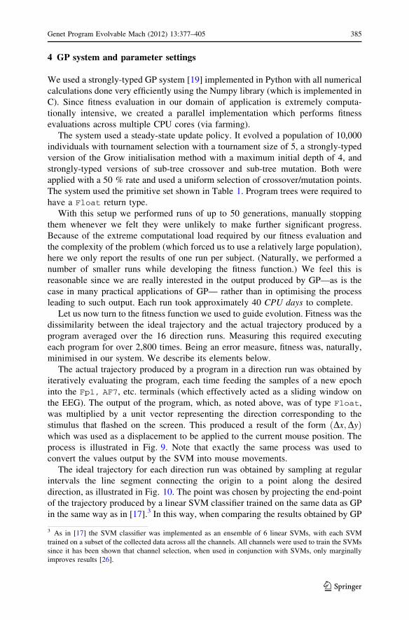
The actual trajectory produced by a program in a direction run was obtained by

iteratively evaluating the program, each time feeding the samples of a new epoch

into the Fp1, AF7, etc. terminals (which effectively acted as a sliding window on

the EEG). The output of the program, which, as noted above, was of type Float,

was multiplied by a unit vector representing the direction corresponding to the

stimulus that flashed on the screen. This produced a result of the form ðDx;DyÞwhich was used as a displacement to be applied to the current mouse position. The

process is illustrated in Fig. 9. Note that exactly the same process was used to

convert the values output by the SVM into mouse movements.

The ideal trajectory for each direction run was obtained by sampling at regular

intervals the line segment connecting the origin to a point along the desired

direction, as illustrated in Fig. 10. The point was chosen by projecting the end-point

of the trajectory produced by a linear SVM classifier trained on the same data as GP

in the same way as in [17].3 In this way, when comparing the results obtained by GP

3 As in [17] the SVM classifier was implemented as an ensemble of 6 linear SVMs, with each SVM

trained on a subset of the collected data across all the channels. All channels were used to train the SVMs

since it has been shown that channel selection, when used in conjunction with SVMs, only marginally

improves results [26].


123

Table 1 Primitive set used in our application

Primitive Output

type

Input type(s) Functionality

0.5, -0.5, 0.1, -0.1,0, 1,…,25

Float None Floating point constants used for

numeric calculations and as array

indexes (see below)

Fp1, AF7, AF3, F1, F3,F5, F7, FT7, FC5, FC3,FC1, C1, C3, C5, T7,TP7, CP5, CP3, CP1, P1,P3, P5, P7, P9, PO7,PO3, O1, Iz, Oz, POz,Pz, CPz, Fpz, Fp2, AF8,AF4, AFz, Fz, F2, F4,F6, F8, FT8, FC6, FC4,FC2, FCz, Cz, C2, C4,C6, T8, TP8, CP6, CP4,CP2, P2, P4, P6, P8,P10, PO8, PO4, O2

Array None Returns an array of 26 samples from

one of the channels in an epoch.

The samples are of type Float.

Channels are named after

corresponding brain regions—F for

frontal, P for parietal, T for

temporal and O for occipital—as

shown below, C representing the

central line between the parietal

and frontal regions. Two-letter

channels are in intermediate

position between two areas

?, -, *, min, max Float (Float, Float) Standard arithmetic operations plus

maximum and minimum on floats

[, \ Bool (Float, Float) Standard relational operations on

floats

if Float (Bool, Float,

Float)

If-then-else function. If the first

argument evaluates to True, then

the result of evaluating its second

argument is returned. Otherwise the

result of evaluating the third

argument is returned

abs Float Float Returns the absolute value of a Float

mean, median, std,Amin, Amax

Float (Float, Float,

Array)

Given a 26-sample Array and two

floats, treat the floats as indices for

the array by casting them to integer

via truncation and then applying a

modulus 26 operation (if the

indices are identical, one is

incremented by 1). Then compute

the mean, median, standard

deviation, minimum or maximum,

respectively, of the samples in the

Array falling between such indices

(inclusive)


123

to those produced by an SVM, we ensured that both had the same ideal trajectories.

The ideal trajectory was sampled in such a way as to have the same number of

samples as the actual trajectory. The comparison between actual and ideal trajectory

was then a matter of measuring the Euclidean distance between pairs of

corresponding points in the two trajectories and taking an average. Notice that

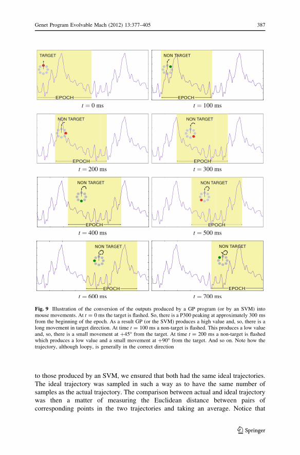
Fig. 9 Illustration of the conversion of the outputs produced by a GP program (or by an SVM) intomouse movements. At t = 0 ms the target is flashed. So, there is a P300 peaking at approximately 300 msfrom the beginning of the epoch. As a result GP (or the SVM) produces a high value and, so, there is along movement in target direction. At time t = 100 ms a non-target is flashed. This produces a low valueand, so, there is a small movement at ?45� from the target. At time t = 200 ms a non-target is flashedwhich produces a low value and a small movement at ?90� from the target. And so on. Note how thetrajectory, although loopy, is generally in the correct direction


123

any detours from the ideal line and any slow-downs in the march along it in the

actual trajectory were strongly penalised with our fitness measure.

5 Experimental results

5.1 Fitness plots, size plots, and best programs

Let us start with some standard statistics for fitness and size. Figures 11 and 12

show the dynamics of the median and best program’s fitness and size in our runs,

respectively. As one can see, in both subjects the median fitness, i.e., the typical

distance of trajectories from the ideal trajectory, started off very badly (note, fitness

scales are logarithmic) with values of around 1,000. Since ideal trajectories are

straight and have a typical length of between 400 and 600 units, this implies that on

average initial programs produced trajectories that were extremely convoluted.

Initial best fitnesses, however, were of the order of 100; so they did show some

degree of motion in the correct direction. For both subjects the median fitness then

rapidly approached the best fitness and they both continued to improve throughout

the runs. For approximately 30 generations for subject 1 and 15–20 generations for

subject 2 after the initial transient, fitness improvements followed a negative

exponential (with a fixed time constant). They then slowed down considerably.

Indeed, this lack of improvement is the reason why we stopped the run for subject 2

after 35 generations. Turning to size, we see that after an initial phase of around 10

generations where programs grew modestly, median and best sizes increased more

rapidly, revealing the presence of bloat.

The best evolved programs, expressed as S-expressions, are as follows (note that

we could not indent them because of their very deep structure):

Ideal Trajectory

GPTrajectory

SVMTrajectory

Fig. 10 Ideal and actual trajectories used in the fitness calculation. Dashed lines indicate pairs ofmatching points. Fitness is the average distance between such points across 16 trajectories. The end pointof the ideal trajectory is computed by projecting the end point of the trajectory produced by an SVM-based flash scorer


123

The programs are also presented in simplified tree form in Fig. 13 (the shading in

the figure will be explained in Sect. 5.4). The programs were first syntactically

simplified replacing expressions of the form (if X ExpA ExpB) with ExpA or ExpB

when X evaluates to the constant True or False, respectively. This happens if

relational operators have both arguments evaluating to a constant, e.g., ([ 0.5

0.0). Then, starting from the leaves, we replaced sub-trees with their median

output if the replacement influenced fitness by less than a pre-determined

acceptance threshold. We used a per-replacement acceptance threshold of 2 % in

Fig. 13. The simplified versions of the best programs used only 11 out of the 64

electrodes for subject 1 and 8 electrodes for subject 2. (The unsimplified versions

subject 2subject 1

Fig. 11 Plots of the median and best fitness versus generation number in our runs. Note that the run forsubject 2 was stopped after 35 generations


123

used 19 electrodes for subject 1 and 21 for subject 2.) This is an advantage over the

SVM, which instead requires all electrodes to be in place.

To evaluate the performance of our best programs we then compared their

outputs (i.e., mouse pointer trajectories) to the outputs produced by the SVM on the

same ERP data (see Sect. 4 for more details on the SVM used). We should note that

the SVM training was orders of magnitude faster than evolving control programs via

GP, taking approximately 1 min per subject.

5.2 Qualitative and statistical analysis of trajectories

Let us start with a qualitative analysis. Figure 14 (top) shows the output produced

by the SVM for each of the direction runs in the training set of each subject (after

the transformation of the SVM scores into ðDx;DyÞ displacements). Ignoring the

small-scales wiggles in the trajectories (which are due to the periodicity of the

flashing stimuli), we see that the SVMs do a reasonably good job at producing

straight trajectories. This feature is the result of the SVM being trained to respond

only when the target stimulus is flashed, and to produce much smaller outputs for all

other (seven) stimuli. A close inspection of the trajectories, however, reveals that

while they are often straight, frequently they do not point exactly in the desired

direction. For example, one of the two trajectories labelled as (-0.7, 0.7) in subject

1 (drawn with a thicker line in Fig. 14 top left) points almost directly upwards

instead of pointing towards the top-left corner of the plot. Also, one of the two

trajectories labelled as (0.7, -0.7) in subject 2 (lower thicker line in Fig. 14 top

right) points almost directly downwards instead of pointing towards the bottom-

right corner of the plot. Finally, one of the two trajectories labelled as (1.0, 0.0) in

subject 2 points (upper thicker line in Fig. 14 top right) towards the top-right corner

of the plot instead of pointing to the right. These biases are the result of the SVM

being a binary classifier. So, while its training algorithm minimises classification

errors, it does not control finely the values of the raw outputs (before thresholding).

subject 2subject 1

Fig. 12 Plots of the median size and the size of the best individual in the population versus generationnumber in our runs


123

Fig. 13 Tree-based representation of the best programs evolved in our runs after syntactic and semanticsimplification (see text) with an acceptance threshold of 2 % and the approximate interpretation of thefunctionality of their main sub-trees


123

As a result SVMs cannot consider an important fact: in order for overall trajectories

to point in the correct direction, the reduced (but often non-zero) output produced in

the presence of flashes of stimuli that are one or two positions before and one or two

positions after a target stimulus must be symmetric (at least on average). Overall,

because of this phenomenon, the SVM produced trajectories which show

insufficient clustering towards the 8 prescribed directions of motion.

Figure 14 (bottom) shows the corresponding trajectories produced by our best

evolved programs. Qualitatively it is clear that these trajectories are more

convoluted. This is to be expected since, unlike SVM, GP did not try to classify

flashes as targets or non-targets. So, there was no explicit bias towards suppressing

the output in the presence of non-target flashes. There was, however, a strong

pressure in the fitness measure towards ensuring that there was overall motion in the

target direction. Also, there was pressure to ensure that the outputs produced for

non-target flashes were such that they either cancelled out or added up in such a way

SVM subject2subject1

GP

Fig. 14 Graphical representation of the 16 sequences of SVM raw scores (top) and the evolved-programraw scores (bottom) for each of our two subjects. The pairs of numbers labelling trajectory endpoints areunit vectors indicating the desired direction of motion. See text for an explanation of thicker lines


123

to contribute to the motion in the target direction, with minimum deviations from

the ideal trajectory. As a result, the trajectories produced by the best programs

evolved by GP were quite close to the ideal line in each of the prescribed directions

of motion. Note, for example, how close the end of the trajectories are to the

corresponding target directions.

To quantitatively verify these observations, we performed statistical comparisons

between the trajectories produced by GP and those produced by SVM.

Let us start with Table 2, which shows the mean, median, standard deviation and

standard error of the mean of the distances between the ideal trajectory and the

actual trajectory recorded in each of the 16 direction runs of each subject. From an

analysis of these data we infer that the best evolved program for subject 1 is, on

average, at least as good as the corresponding SVM, while the best evolved program

for subject 2 is definitely superior to the SVM. Note that for both subjects the

trajectories produced by GP have a much lower standard deviation than those

produced by SVMs. This is an indication that the evolved programs show a much

more consistent behaviour and are likely less sensitive to artifacts than SVMs.

Since for each direction run we have both the trajectory produced by the

SVM and the trajectory produced by an evolved program, we can apply paired-

data statistics to evaluate whether the results obtained by the evolved controllers

are superior to those obtained by the SVM. To test this, we applied the one-

sided Wilcoxon signed rank test for paired data to the 16 trajectories of each

subject. Table 3 reports the p-values obtained. These confirm that the evolved

programs produce trajectories that are significantly better than those produced by

SVM for subject 2 and are approximately on par with SVM in the case of

subject 1.

Table 2 Statistical comparison between SVM and evolved solutions: basic statistics of the distribution

of distances between ideal and actual mouse trajectories

Subject Program Mean Median Standard deviation Standard error

1 GP 50.813 44.367 17.440 4.503

SVM 52.638 43.709 30.550 7.888

2 GP 38.424 37.797 10.030 2.590

SVM 69.766 59.997 34.518 8.913

Boldface indicates superior results

Table 3 Statistical comparison between SVM and evolved solutions: p-values for the one-sided Wil-

coxon signed rank test for paired data

Subject p-value (is GP better than SVM?)

1 0.430

2 0.000

Boldface indicates statistical significance


123

5.3 Effects of smoothing trajectories

Naturally, the more pronounced swirls present in the trajectories produced by the

evolved programs may be a distraction for a user. It is, however, easy to remove

them by post-processing the mouse movements ðDxi;DyiÞ produced by the system

via a smoothing function. To study the benefits and drawbacks of this, we have used

an exponential infinite-impulse-response filter of the form:

ðDxsi ;Dys

i Þ ¼ a � ðDxi;DyiÞ þ ð1� aÞ � ðDxsi�1;Dys

i�1Þ;

with a = 1/30 and initialisation ðDxs0;Dys

0Þ ¼ ðDx0;Dy0Þ; that has a smoothing effect

which is effectively equivalent to associating a momentum to the mouse cursor.

Figure 15 shows the resulting trajectories. Clearly smoothing improves signif-

icantly the straightness of the trajectories produced by evolved programs, thereby

removing the potential negative effects of the swirls in the raw trajectories.

Smoothing, of course, does not improve the directional biases in the trajectories

produced by the SVMs, although it makes them more rectilinear.

Smoothing has also some effects on the statistics of the distances from ideal

trajectories. Table 4 reports the mean, median, standard deviation and standard error

of the mean of the distances between the ideal trajectory and the actual trajectory

(after smoothing) for each of the 16 direction runs of each subject. As one can see

by comparing the values in the table with those in Table 2, for subject 1, smoothing

produces a slight worsening of the average performance for GP and a much bigger

one for the SVM. The most likely cause of this is the transient due to the

initialisation of the smoothing filter. Because ðDxs0;Dys

0Þ ¼ ðDx0;Dy0Þ and a is very

small, the initial movement vector ðDx0;Dy0Þ influences the filter’s output for many

time steps. This influence may be positive if ðDx0;Dy0Þ is in the target direction.

However, if ðDx0;Dy0Þ is not in the target direction (which is relatively likely), the

transient provokes unnecessary detours from the ideal trajectory.

So, in a good subject, like subject 1, where trajectories were already relatively

straight, the addition of the smoothing filter may bring no benefits or even be

deleterious in relation to distances from ideal trajectories. The drop in performance

is more limited in the case of GP trajectories, because it is compensated for by the

total elimination of the large swirls which characterised such trajectories and made

them deviate from the ideal line.

For a relatively poor subject, like subject 2, whose raw trajectories present more

artifacts and can thus benefit more from the smoothing, the negative effects of the

transient in the filter’s output are outweighed by the benefits. Indeed, the data for

subject 2 show that, in the presence of smoothing, the mean and median are

marginally improved for the evolved solutions, while for the SVM there is a slight

improvement in the mean but a worsening for the median.

Table 5 reports the p-values obtained when we analysed the smoothed

trajectories using a one-sided Wilcoxon signed rank test for paired data. These

confirm our previous analysis. The evolved program for subject 2 remains

statistically significantly superior to the corresponding SVM. In addition, smoothing

makes the differences between the trajectories produced by GP and those produced

by SVM almost statistically significant also for subject 1.


123

In summary, while smoothing either does not (or only marginally) improve

things in relation to our objective measure, it still brings much benefit in terms of

the users not being distracted by the swirls of the raw trajectories.

As a final note on the issue of smoothing, in Sect. 2 we indicated that in [17]

Eq. (1) was used to smooth and integrate the raw trajectories produced by an SVM.

SVM + Smoothing subject 2subject 1

GP + Smoothing

Fig. 15 Trajectories produced by SVM and GP after the application of a low-pass filter

Table 4 Statistical comparison between the trajectories produced by the SVM and GP after low-pass

filtering: basic statistics of the distribution of distances between ideal and actual mouse trajectories

Subject Program Mean Median Standard Deviation Standard Error

1 GP 52.337 47.204 17.888 4.619

SVM 62.652 52.154 27.060 6.987

2 GP 37.453 37.377 9.739 2.515

SVM 68.305 68.191 33.853 8.741



123

In Fig. 16 we show the trajectories produced by such a procedure applied on the raw

outputs of the SVM for the two subjects in this study (reported at the top of Fig. 14).

Note the considerable similarity between Figs. 15 (top) and 16, the only difference

being the slightly more rugged nature of the former. This suggests that this

procedure is effectively equivalent to a low-pass filtering of trajectories.

5.4 Interpretation of evolved programs

While the results reported in the previous sections are very encouraging, it is also

important to see what lessons can be learnt from the evolved programs themselves.

The programs are reproduced with shadings to aid interpretation in Fig. 13.

Looking at the program evolved for subject 1, we see that its output is simply the

mean of a consecutive block of samples taken from channel P8. The choice of P8 is

quite appropriate, since this and other parietal channels are often the locations where

the P300 has maximum amplitude. The decision to select sample 15 (which

corresponds to 469 ms after the presentation of the stimulus) as one of the two

extremes of the averaging block is also correct, since this sample falls right in the

middle of typical P300 waves. The sample marking the other end of the averaging

block is the result of a more elaborate choice determined by three cascaded if

SVM + Standard Integratorsubject 1 subject 2

Fig. 16 Trajectories produced by the SVM followed by the standard integrator in Eq. (1)

Table 5 Statistical comparison between the trajectories produced by the SVM and GP after low-pass

filtering: p-values for the one-sided Wilcoxon signed rank test for paired data

Subject p-value (is GP better than SVM?)

1 0.106

2 0.001

Boldface indicates statistical significance. Italics indicates a result close to significance


123

statements. Effectively this sample can take four different values: 0 (0.5 is truncated

to 0), 4 (125 ms), 10 (313 ms) or 20 (625 ms). Sample 0 is chosen when the

leftmost shaded sub-tree in Fig. 13 (left) returns True. Careful analysis has clarified

that this tree is specialised in detecting near targets, i.e., non-target flashes that

immediately precede or follow the flashing of a target. When not in the presence of

a near target, sample 4 is chosen if the second shaded sub-tree returns True.

Analysis suggests that this sub-tree is a negated detector of eye-blinks in the early

part of the data. If an eye-blink is detected, then control passes to the last if in the

chain which moves away the averaging window from the early samples, forcing the

average to cover either the range 10–15 or the range 15–20 depending on the

likelihood of finding a target-related P300 in the corresponding time windows

(313–469 and 469–625 ms, respectively). This decision is taken by the right-most

shaded sub-tree.

A pseudo-code implementation of this evolved solution is shown in Algorithm 1.

Turning now to the program evolved for subject 2, we see that it too uses the

strategy of returning the average of a particular channel, FC2 in this case. Here the

average is between a fixed sample (13, corresponding to 406 ms) and a second

sample which is computed based on a number of conditions. In this case, the output

is clipped to the value 13. We think this clipping is an eye-blink handling strategy.

Since channel FC2 is relatively frontal, the system needs to prevent eye-blinks from

producing disastrous off course mouse movements. By clipping the output to 13,

eye-blinks (which typically produce huge voltages for many hundreds of

milliseconds, i.e., many stimulus flashes) will cause the pointer trajectory to loop

(following the perimeter of a small regular octagon), thereby never going too far off

course. Note that the choice of sample 13 (406 ms) as one extreme for the windows

where the mean is computed is quite appropriate since this sample, too, falls in the

middle of typical P300s.

The values used as the second extreme of the averaging window depends on the

result of the comparison carried out in the left-most shaded sub-tree in Fig. 13

(right). In this subtree electrode Iz (which is at the base of the skull) has a prominent

Algorithm 1 Pseudo code of mouse-control program evolved for subject 1

1: if NearTarget() then

2: OtherLimit = 0 ms

3: else if !EyeBlink() then


5: else if Target() then


7: else


9: end if

10: return mean(OtherLimit, 469 ms, P8)


123

role. The subtree is effectively a detector for neck movements and other muscular

artifacts in the early samples of an epoch. If one such artifact is detected, the second

extreme for the mean is based on the calculation (mean 0.1 308 CP2), which is

internally transformed into (mean 0 22 CP2). Note that sample 22 corresponds to

688 ms. The stronger the effect of the artifact on centro-parietal areas, the more the

resulting sample moves away from the beginning of the epoch, thereby avoiding the

influence of spurious data in the determination of the program output. If no early

muscle artifact is detected then the second extreme of the averaging block is either 1

(32 ms) or 19 (594 ms).

The decision about which sample to use is essentially made by a second artifact

detection subtree (right-most shaded tree in Fig. 13 (right). When activated, this

checks for muscle artifacts over a wider range of samples (including the end of the

epoch). If none is detected, this causes a domino effect involving the five if

statements connecting the subtree to the mean-over-FC2 instruction near the top of

the program, with all such if statements returning 19. Sample 19 is then used as the

second extreme of the averaging window for FC2. In the absence of eye-blinks, the

output of the program is thus the average of FC2 over the range 406–594 ms. This

makes complete sense since the range effectively covers most of the energy in the

P300 wave.

A pseudo-code implementation of the evolved solution is shown in Algorithm 2.

6 Generalisation

There are two main questions in relation to the ability to generalise of the evolved

controllers. The first question is whether a controller evolved for one subject will

work for a different subject. The second question is whether a controller evolved

using training data from one subject would work on test data from the same subject.

We discuss these issues in this section.

Algorithm 2 Pseudo code of mouse-control program evolved for subject 2

1: if EarlyArtifact() then

2: OtherLimit = mean(0 ms, 688 ms, CP2)

3: else

4: if OtherArtifact() then


6: else


8: end if

9: end if

10: RawOutput = mean(OtherLimit, 406 ms, FC2)

11: return min(13, RawOutput)


123

6.1 Generalisation across subjects

As we have seen previously, the controllers evolved by our GP system and the

SVMs used for reference are specialised to each specific subject. There is enormous

inter-subject variability in ERPs and artifacts, both in terms of location of activity

on the scalp and the time at which such activity occurs. These are mainly caused by

individual differences on how brains respond to stimuli. As a result, there is little

hope that a controller specialised for one subject will work well for a different

subject. For those familiar with speech recognition, it would be as implausible as

expecting that a system trained with a female soprano voice would properly

recognise the speech of a male bass voice. For these reasons subject-dependency

and lack of generalisation beyond a subject are, literally, ubiquitous in BCI

wherever machine learning technology is adopted. For example, all systems

described in Sect. 2 were trained on a user-by-user basis.

As a demonstration of the kind of performance one may obtain when applying a

controller evolved using the data from one subject to the data of another subject, we

tested subject 1’s controller on the data of subject 2 and vice versa obtaining the

results reported in Tables 6 and 7. As expected, results are very poor compared with

those of the reference SVMs (trained on the test-subject data).

6.2 Generalisation within subjects

The second issue related to generalisation—whether a controller evolved using

training data from a subject works on test data from that subject—is a particularly

important one. The standard approach in machine learning is to divide the data

available into a training set and an independent test set. The prerequisite for this is

Table 6 Statistical comparison between the output of the SVM trained with data from a subject and the

solution evolved using the data from the other subject: basic statistics of the distribution of distances

between ideal and actual mouse trajectories


1 GP 3100.944 807.342 5020.364 1296.252

SVM 52.638 43.709 30.550 7.888

2 GP 1553.989 511.953 3853.857 995.062

SVM 69.766 59.997 34.518 8.913



solution evolved using the data from the other subject: p-values for the one-sided Wilcoxon signed rank

test for paired data

Subject p-value (is SVM trained on a subject’s data better than GP tested on the same data but trained

on the other subject’s data?)

1 0.000

2 0.000


123

that, after the split, one is still left with sufficiently large and representative training

and test sets.

In BCI, data sets can never be very large, because their acquisition is a labour

intensive process involving human subjects. When subjects start becoming tired,

their attention levels drop and, as a consequence, their brain signals start changing.

These changes include much reduced or even absent P300s where one would

normally have robust ones, which is naturally a key problem for P300-based BCIs.

Also, as subjects become tired they tend to produce more muscular artifacts, which

are generally a very big problem for BCI. To counteract this, it is common practice

to give subjects regular breaks, offering refreshments, and so on. However, after

about 1 h of experimentation (excluding subject preparation, which takes approx-

imately 30 min) subjects wear out. Degradation of signals is also induced by the

drying out of the gel used to ensure good electrical connection between scalp and

electrodes, which starts becoming a problem after a couple of hours since

deployment.

Because of the limited size of BCI datasets, it is very rarely the case that one can

split a single-subject dataset into two representative training and test sets. This was

the case also for the data acquired from our subjects. Particularly difficult is

ensuring that both sets include a representative set of artifactual epochs (as well as

normal ones), which are rarer but tend to occur in fits. So, to evaluate whether

systems generalise, BCI researchers tend to use a k-fold cross validation approach

with values of k around 10, to ensure each fold has a training set as large as possible.

A problem with these approaches is that they can only effectively be adopted if

the machine learning algorithm is reasonably fast. However, as we explained in

Sect. 4, our GP runs were extremely computationally intensive, making a cross-

validation approach non-viable in our case. For example, an 8-fold cross validation

would have required approximately 280 CPU days per subject.

These are the reasons why we decided to include all of the data available to us in

the training set. In order to evaluate whether the evolved controllers would

generalise to unseen data, for each subject we generated an artificial test set by

suitably modifying (via morphing) the training data. The approach is described in

the next section.

6.2.1 Monte Carlo morphing

In the absence of a separate training set, it is possible to use Monte Carlo

simulations to ‘‘replay’’ the training data in a meaningful but significantly different

way so as to simulate a real testing situation. For example, we used this strategy in

[20]. The key to a successful simulation, however, is that the reply must be

meaningful, i.e., the output of a system must be influenced by the differences

introduced in the replay. In [20] we randomised the order of the replay of epochs,

since the method we were studying was influenced by the specific sequence in

which epochs were presented. The controllers evolved by GP in this paper, however,

produce exactly the same output in the presence of the same input epoch,

irrespective of the order in which epochs are presented to them. So, a different

approach is needed.


123

The algorithm we came up with is based on the idea of generating new data by

morphing each original ERPs towards the ERP recorded in another epoch (randomly

selected with the constraint that it must correspond to a flash of a stimulus in the

same direction as that of the original ERP). The morphing is obtained via the

formula

ERPtest set epoch ¼ a� ERPtraining set epoch þ ð1� aÞ � ERPother compatible training set epoch

ð2Þ

where a is a value drawn uniformly at random from the interval [0.0, 1.0]. This

morphing formula was used for the epochs in all 16 direction runs of the training set

of each subject, resulting in a corresponding test set including 16 direction runs of

the same duration as the original, but with significantly different ERP shapes.

Details on the generation of each test direction run are provided in Algorithm 3.

Test sets created with this algorithm are particularly difficult to classify if a

system does not generalise properly. This is for two reasons. Firstly, because of our

choice for the distribution of the stochastic variable a, Eq. (2) typically produces

ERPs which are radically different from the two ‘‘parent’’ ERP. Secondly, the

resulting test sets include approximately twice as many artifactual epochs as the

original. This second point requires a bit more explanation.

The amplitude of the EEG signals recorded during an eye blink, a neck

movement, etc., can be one or two orders of magnitude bigger that ordinary ERPs.

As a result of this and of the fact that E[a] = 0.5, if an artifact-free epoch is

combined with one including artifacts using Eq. (2), the resulting test epoch will

likely show the very large voltages observed in artifactual epochs. For example, let

us consider a typical non-artifactual epoch presenting a P300 and let us imagine that

the voltage recorded at sample 10 (313 ms from stimulus onset) is 6 lV. Let us now

imagine that such epoch is morphed using an a = 0.53 with an epoch that presents a

muscle artifact resulting in a voltage of 300 lV at sample 10. Applying Eq. (2) one

Algorithm 3 Pseudo code of the test set generation algorithm used to verify the generalisation of the

evolved controllers

1: for epoch = 0...numEpochsDirRun-1 do

2: direction = epoch mod 8

3: otherEpoch = (randint(0, numEpochsDirRun - 1) div 8) * 8 ?direction

4: if otherEpoch[= numEpochsDirRun then

5: otherEpoch = otherEpoch - 8

6: end if

7: alpha = random()

8: output[epoch] = alpha * dirEpoch[epoch] ? (1 - alpha) *dirEpoch[otherEpoch]

9: end for

10: return output


123

finds that the output epoch will present a voltage of approximately 144 lV at

sample 10, making it indistinguishable from an artifactual epoch.

Naturally, this also happens if one morphs two artifactual epochs together. It is

only when a non-artifactual epoch is combined with a second non-artifactual epoch

that the resulting signals will look non-artifactual. As a consequence, if ptrain is the

proportion of epochs containing artifacts, the proportion of test-set epochs

containing artifacts, ptest, is expected to be:

ptest ¼ 1� Prftest epoch is artifact freeg ¼ 1� ð1� ptrainÞ2 ¼ 2ptrain � p2train

So, for sufficiently small ptrain (e.g., ptrain B0.2, which is certainly the case in our

training sets), we have that ptest % 2ptrain. That is, as indicated above, the fraction ofartifactual epochs in the test set is approximately double that of the training set.

6.2.2 Within-subject generalisation results

The results obtained when applying our evolved detectors to morphed test sets

constructed as described above are summarised in Tables 8 and 9. To provide an

absolute reference, we still compare the performance of evolved programs to that

obtained by the corresponding SVM on the original data.

The first thing to note is that, while GP results are inferior to those obtained in the

training set (see Table 2), they are still very good and nowhere near the no-

generalisation-across-subjects results reported in Table 6. Also, as indicated in

Table 9, while the GP results appear to be slightly inferior to those of the reference

SVM, the difference is actually not statistically significant.

Overall the within-subject generalisation shown by the solutions evolved by GP

is very good, particularly considering that our test set effectively contains twice as

many artifactual epochs as the original training set.


solution evolved using a test set generated via morphing using data from the same subject: basic statistics

of the distribution of distances between ideal and actual mouse trajectories


1 GP 65.489 63.670 25.542 6.595

SVM 52.638 43.709 30.550 7.888

2 GP 74.281 67.687 35.530 9.174

SVM 69.766 59.997 34.518 8.913



solution evolved using a test set generated via morphing using data from the same subject: p-values for

the one-sided Wilcoxon signed rank test for paired data

Subject p-value (is SVM better than GP?)

1 0.116

2 0.281


123

7 Conclusions

Brain–computer interfaces are an exciting research area that, 1 day, will hopefully

turn the dream of effortlessly and efficiently interpreting users’ commands directly

from electrical brain signals into reality. Progress is constantly made in BCI but it is

slowed down by many factors, including the noise present in brain signals, the

variability of EEG signals and ERPs across subjects, muscular artifacts and the

inconsistency and variability of user attention and intentions.

Recent research [8, 16] has shown that genetic algorithms and support vector

machines can be of great help in the selection of the best channels, time steps and/or

filtering kernels to use for the control of an ERP-based BCI mouse. In this paper we

proposed the use of GP as a means to evolve BCI mouse controllers—a very

difficult task that has never been attempted before.

Our objective was to synthesise complete systems, which analyse electroen-

cephalographic signals and directly transform them into pointer movements. The

only input we provided in this process was the set of visual stimuli to be used to

generate recognisable brain activity. Note that there is no high-performance, human-

designed system for ERP-based mouse pointer control in BCI. There simply aren’t

any design guidelines for a domain such as this. This is why all but one of the

systems of this kind reported in the literature use some form of machine learning

(the system that did not use machine learning [6] had very poor performance).

The results of the experiments with our approach reported in this paper show that

GP can produce very effective BCI mouse controllers which include clever

mechanisms for artifact reduction. The picture emerging from our experiments is

that not only has GP been successful in the automated design of a control system for

a BCI mouse, but it has also been able to perform at least on par with (if not better

than) SVMs—which until now have been considered perhaps the best machine-

learning technology available for BCI—using only a fraction of the electrodes

needed by them. Additionally, GP produces controllers that can be understood and

from which we can learn new effective strategies for BCI.

All this suggests that our evolved systems are at, or above, state-of-the-art,

indicating that, perhaps, they qualify for the attribute of human-competitive, in the

sense indicated by Koza (e.g., see [21]).

Naturally, there are also limitations to the techniques reported in this paper.

Firstly, as we discussed in Sect. 6, there is the issue of generalisation of the evolved

controllers. While we are confident that our controllers generalise to unseen data

from the subject they were evolved for, it would be important to be able, 1 day, to

evolve controllers that go beyond subject-dependency typical of BCI. Also, there is

the issue of the long training times that GP requires, which are not required by the

SVM here and in [17] nor were required by the GA in [8, 16].

As a first attempt to address these issues, we have started to explore hybrid

systems where one SVM or an ensemble of SVMs is trained on a per-subject basis,

but where a trajectory integrator which is applicable across subjects is evolved by

GP [22, 23]. In these systems, once evolved, the GP integrator can be used over and

over again. So, only the SVM training is required to get a working system with a

new subject. Results so far with this idea have been promising.


123

Naturally, there are many other alternative avenues we hope to be able to explore

in future research. For example, as suggested by one of our reviewers, it would

make sense to encapsulate the trees shown within the shade regions in Fig. 13 and

provide them as primitives to a GP system, thereby making its task much easier (and

hopefully evolution times much shorter). Also, with minor variations of the

principles used in this paper, it would be possible to try 3-D pointer movement and

3-D navigation in virtual environments.

Acknowledgments We would like to thank EPSRC (grant EP/F033818/1) for financial support. We

would also like to thank the reviewers for their very useful comments.

References

1. L.A. Farwell, E. Donchin, Talking off the top of your head: toward a mental prosthesis utilizing

event-related brain potentials. Electroencephalogr. Clin. Neurophysiol. 70, 510–523 (1988)

2. J.R. Wolpaw, D.J. McFarland, G.W. Neat, C.A. Forneris, An EEG-based brain–computer interface

for cursor control. Electroencephalogr. Clin. Neurophysiol. 78, 252–259 (1991)

3. G. Pfurtscheller, D. Flotzinger, J. Kalcher, Brain–computer interface: a new communication device

for handicapped persons. J. Microcomput. Appl. 16(3), 293–299 (1993)

4. N. Birbaumer, N. Ghanayim, T. Hinterberger, I. Iversen, B. Kotchoubey, A. Kbler, J. Perelmouter,

E. Taub, H. Flor, A spelling device for the paralysed. Nature 398, 297–298 (1999)

5. J.R. Wolpaw, D.J. McFarland, Control of a two-dimensional movement signal by a noninvasive

brain-computer interface in humans. Proc. Natl. Acad. Sci. 101(51), 17849–17854 (2004)

6. J.B. Polikoff, H.T. Bunnell, W J. Borkowski Jr., Toward a P300-based computer interface, in

Rehabilitation Engineering and Assistive Technology Society of North America (RESNA’95)(Arlington, Va) (Resna Press, 1995), pp. 178–180

7. F. Beverina, G. Palmas, S. Silvoni, F. Piccione, S. Giove, User adaptive BCIs: SSVEP and P300

based interfaces. PsychNol. J. 1(4), 331–354 (2003)

8. L. Citi, R. Poli, C. Cinel, F. Sepulveda, P300-based BCI mouse with genetically-optimized analogue

control. IEEE Trans. Neural Syst. Rehabil. Eng. 16, 51–61 (2008)

9. M. Salvaris, C. Cinel, R. Poli, Novel sequential protocols for a ERP based BCI mouse. 5th inter-

national IEEE EMBS neural engineering conference, IEEE Press, 2011, pp. 352–355

10. J.R. Koza, Genetic Programming: On the Programming of Computers by Means of Natural Selection.

(MIT Press, Cambridge, MA, USA, 1992)

11. R. Poli, W. B. Langdon, N. F. McPhee, A field guide to genetic programming (2008), Published via

http://lulu.com and freely available at http://www.gp-field-guide.org.uk (With contributions by

J. R. Koza)

12. J. Donoghue, Connecting cortex to machines: recent advances in brain interfaces. Nat. Neurosci. 5,

1085–1088 (2002)

13. P. Comon, Independent component analysis, a new concept? Signal Process. 36, 287–314 (1994)

14. S. Makeig, A.J. Bell, T.-P. Jung, T.J. Sejnowski, Independent component analysis of electroen-

cephalographic data, in Advances in Neural Information Processing Systems, vol. 8, ed. by D S.

Touretzky, M.C. Mozer, M.E. Hasselmo (The MIT Press, Cambridge, MA, 1996), pp. 145–151

15. C. Cortes, V. Vapnik, Support-vector networks. Mach. Learn. 20(3), 273–297 (1995)

16. R. Poli, L. Citi, F. Sepulveda, C. Cinel, Analogue evolutionary brain computer interfaces. IEEE

Comput. Intell. Mag. 4, 27–31 (2009)

17. M. Salvaris, C. Cinel, R. Poli, L. Citi, F. Sepulveda, Exploring multiple protocols for a brain–

computer interface mouse, in Proceedings of 32nd IEEE EMBS Conference, Buenos Aires,

pp. 4189–4192, Sept 2010

18. J. Wolpaw, N. Birbaumer, W. Heetderks, D. McFarland, P. Peckham, G. Schalk, E. Donchin,

L. Quatrano, C. Robinson, T. Vaughan, Brain–computer interface technology: a review of the first

international meeting. Rehabil. Eng. IEEE Trans. 8(2), 164–173 (2000)

19. D.J. Montana, Strongly typed genetic programming. Evol. Comput. 3(2), 199–230 (1995)


123

http://lulu.com

http://www.gp-field-guide.org.uk

20. L. Citi, R. Poli, C. Cinel, Documenting, modelling and exploiting P300 amplitude changes due to

variable target delays in Donchin’s speller. J. Neural Eng. 7(5), 056006 (2010)

21. J. R. Koza, Human-competitive results produced by genetic programming. Genet. Programm.Evolvable Mach. 11, 251–284, Sept 2010. Tenth Anniversary Issue: Progress in Genetic Program-

ming and Evolvable Machines

22. R. Poli, M. Salvaris, C. Cinel, Evolutionary synthesis of a trajectory integrator for an analogue brain–

computer interface mouse, in Applications of Evolutionary Computation (EvoApplications),vol. 6624 of Lecture Notes in Computer Science, ed. by C.D. Chio, S. Cagnoni, C. Cotta, M. Ebner,

A. Ekart, A. Esparcia-Alcazar, J.J.M. Guervos, F. Neri, M. Preuss, H. Richter, J. Togelius, G.N.

Yannakakis (Springer, Berlin, 2011), pp. 214–223

23. R. Poli, M. Salvaris, C. Cinel, Evolution of an effective brain-computer interface mouse via genetic

programming with adaptive Tarpeian bloat control, in Genetic Programming Theory and Practice IX,

ed. by R. Riolo, E. Vladislavleva, J.H. Moore (Springer, New York, 2011), forthcoming

24. R. Poli, M. Salvaris, C. Cinel, Evolution of a brain–computer interface mouse via genetic pro-

gramming, in Proceedings of Genetic Programming—14th European Conference, EuroGP, no. 6621in Lecture Notes in Computer Science, ed. by S. Silva, J.A. Foster, M. Nicolau, P. Machado,

M. Giacobini (Springer, Berlin, 2011) pp. 203–214

25. W.S. Pritchard, Psychophysiology of P300. Psychol. Bull. 89, 506–540 (1981)

26. A. Rakotomamonjy, V. Guigue, BCI competition III: dataset II—ensemble of SVMs for BCI P300

speller. IEEE Trans. Biomed. Eng. 55, 1147–1154 (2008)


123

A genetic programming approach to the evolution of brain–computer interfaces for 2-D...

Documents

Transcript of A genetic programming approach to the evolution of brain–computer interfaces for 2-D...