A genetic algorithms approach to growth phase...
22
International Journal of Forecasting 18 (2002) 625–646 www.elsevier.com / locate / ijforecast A genetic algorithms approach to growth phase forecasting of wireless subscribers 1 ,2 * Rajkumar Venkatesan ,V. Kumar ING Center for Financial Services, School of Business, University of Connecticut, Storrs, CT 06269-1041, USA Abstract In order to effectively make forecasts in the telecommunications sector during the growth phase of a new product life cycle, we evaluate performance of an evolutionary technique: genetic algorithms (GAs), used in conjunction with a diffusion model of adoption such as the Bass model. During the growth phase, managers want to predict (1) future sales per period, (2) the magnitude of sales during peak, and (3) when the industry would reach maturity. At present, reliable estimation of parameters of diffusion models is possible, when sales data includes the peak sales also. Cellular phone adoption data from seven Western European Countries is used in this study to illustrate the benefits of using the new technique. The parameter ¨ estimates obtained from GAs exhibit good consistency comparable to NLS, OLS, and a naıve time series model when the entire sales history is considered. When censored datasets (data points available until the inflection point) are used, the proposed technique provides better predictions of future sales; peak sales time period, and peak sales magnitude as compared to currently available estimation techniques. 2002 International Institute of Forecasters. Published by Elsevier Science B.V. All rights reserved. Keywords: New product diffusion-estimation; Genetic algorithms; Telecommunication industry; Bass model Forecast). Specifically the sales of mobile wire- 1. Introduction less phones worldwide increased by 46% in The telecommunication industry has ex- year 2000. Also, by the end of 2001, European perienced rapid growth in the recent years and Mobile Communications (EMC) forecasts world is forecasted to exceed $790B in revenues by cellular subscriptions to top the one billion 2003 (2000 Multimedia Telecommunications mark, up from 728 million at year end 2000. The sustained tremendous growth in the wire- less communications industry over the past *Corresponding author. Tel.: 11-860-486-1086; fax: 11-860-486-8396. decade also aggravates the need for accurate E-mail addresses: [email protected] (R. forecasts of future growth potential. The Venkatesan), [email protected] (V. Kumar). ubiquitous product life cycle would suggest that 1 Rajkumar Venkatesan is an Assistant Professor in Market- a phase of consolidation and decline in growth ing. 2 is imminent. In that case, when is it supposed to V. Kumar (VK) is the ING Chair Professor and Executive happen? Director. 0169-2070 / 02 / $ – see front matter 2002 International Institute of Forecasters. Published by Elsevier Science B.V. All rights reserved. PII: S0169-2070(02)00070-5
Transcript of A genetic algorithms approach to growth phase...

International Journal of Forecasting 18 (2002) 625–646www.elsevier.com/ locate/ ijforecast
A genetic algorithms approach to growth phase forecasting ofwireless subscribers
1 ,2*Rajkumar Venkatesan , V. KumarING Center for Financial Services, School of Business, University of Connecticut, Storrs, CT 06269-1041,USA
Abstract
In order to effectively make forecasts in the telecommunications sector during the growth phase of a new product lifecycle, we evaluate performance of an evolutionary technique: genetic algorithms (GAs), used in conjunction with a diffusionmodel of adoption such as the Bass model. During the growth phase, managers want to predict (1) future sales per period,(2) the magnitude of sales during peak, and (3) when the industry would reach maturity. At present, reliable estimation ofparameters of diffusion models is possible, when sales data includes the peak sales also. Cellular phone adoption data fromseven Western European Countries is used in this study to illustrate the benefits of using the new technique. The parameter
¨estimates obtained from GAs exhibit good consistency comparable to NLS, OLS, and a naıve time series model when theentire sales history is considered. When censored datasets (data points available until the inflection point) are used, theproposed technique provides better predictions of future sales; peak sales time period, and peak sales magnitude as comparedto currently available estimation techniques. 2002 International Institute of Forecasters. Published by Elsevier Science B.V. All rights reserved.
Keywords: New product diffusion-estimation; Genetic algorithms; Telecommunication industry; Bass model
Forecast). Specifically the sales of mobile wire-1 . Introductionless phones worldwide increased by 46% in
The telecommunication industry has ex- year 2000. Also, by the end of 2001, Europeanperienced rapid growth in the recent years and Mobile Communications (EMC) forecasts worldis forecasted to exceed $790B in revenues by cellular subscriptions to top the one billion2003 (2000 Multimedia Telecommunications mark, up from 728 million at year end 2000.
The sustained tremendous growth in the wire-less communications industry over the past*Corresponding author. Tel.:11-860-486-1086; fax:
11-860-486-8396. decade also aggravates the need for accurateE-mail addresses: [email protected](R. forecasts of future growth potential. The
Venkatesan),[email protected](V. Kumar). ubiquitous product life cycle would suggest that1Rajkumar Venkatesan is an Assistant Professor in Market- a phase of consolidation and decline in growthing.2 is imminent. In that case, when is it supposed toV. Kumar (VK) is the ING Chair Professor and Executive
happen?Director.
0169-2070/02/$ – see front matter 2002 International Institute of Forecasters. Published by Elsevier Science B.V. All rights reserved.PI I : S0169-2070( 02 )00070-5

626 R. Venkatesan, V. Kumar / International Journal of Forecasting 18 (2002) 625–646
Sales forecasts during the early stages of a just the time since a product has been intro-product life cycle are critical to both new duced in the market for making reliable fore-product managers and academicians. The casts of the future sales of the innovation. Ingrowth phase of the product life cycle is char- addition to providing reliable forecasts, the Bassacterized by high growth in sales and market model has attractive behavioral implicationsexpansion. Also, the marketing strategy in the regarding customer motivation that could assistgrowth phase is characterized by heavy adver- managerial decision-making.tising as compared to heavy promotions in the Since its introduction, the Bass (1969) modelmaturity /decline stage (Kotler, 2000). Given of innovation adoption has spawned a widethe implications to marketing strategy, predict- range of applications and models that explaining the future sales during the growth phase is the rate of adoption of an innovation (Bayus,of paramount importance. In addition to predict- 1992), the effect of marketing mix variables oning the future sales of the product, managers the market potential and rate of adoption of anneed to know when the product would reach innovation (Bass, Krishnan, & Jain, 1994; Jainmaturity and what the value of sales would be at & Rao, 1990; Kalish, 1983; Bass, 1980; Robin-maturity. Accurate knowledge about the time to son & Lakhani, 1975), and diffusion of innova-peak sales helps managers deduce the growth tions in multiple markets (Krishnan, Bass, &rate of their markets, and the marketing mix Kumar, 2000; Kumar, Ganesh, & Echambadi,necessary to accelerate the sales of their new 1998; Takada & Jain, 1991). Even the basicinnovation. Appropriate forecasts of future Bass diffusion model has been modified togrowth potential are essential for proper man- accommodate for time-varying parameters, flex-agement of resources, and further have im- ibility in the shape of the diffusion pattern, andportant profit implications. evaluating marketing strategies that are effective
Several micro-level telecommunications de- in various stages of the product life cycle, andmand models have been proposed (Fildes, influence of another country on one country’s2002) that accommodate characteristics such as diffusion (Kumar & Krishnan, 2002; Ganesh,network effects, price elasticity, government Kumar & Subramaniam, 1997). Forecasting ofregulations, incentive structures and product future sales, a critical application of the Bassquality. The micro-level models seem to work diffusion model, has received little or no atten-well in established markets and for new prod- tion because researchers are faced with difficul-ucts /services the reliance is more on qualitative ties in using the Bass model for this purposemeasures such as expert /consumer opinion. In (Parker, 1994). The forecasting of future salesaddition to micro-level models, managers are of a new product before the inflection point inalso interested in forecasting the macro-level the product life cycle is reached is a particularlygrowth for a new market over a fixed time critical drawback (Mahajan, Muller, & Bass,horizon in order to assist decision-making and 1990).strategy development. The macro-level models Ordinary Least Squares (OLS), Maximumthat are used need to be parsimonious and are Likelihood, and Non-linear Least Squaresmostly used in combination with micro-level (NLS) procedures have been proposed in themodels for decision-making. Several macro- literature for estimating the parameters in a Basslevel time series models including logistic diffusion model. However each technique hasgrowth curves have been proposed to predict the its own shortcomings with respect to providingfuture category level sales of an innovation. The reliable and accurate forecasts of product sales/Bass (1969) model is one such model that uses growth. The estimates based on OLS are biased

R. Venkatesan, V. Kumar / International Journal of Forecasting 18 (2002) 625–646 627
because OLS (1) assumes a discrete process for unreliable. In the continuous time framework,data generated from a continuous process, (2) the reliable estimation of the Bass model issuffers from multicollinearity, and (3) does not possible only when the inflection point in thegenerate standard errors directly forp, q, andm product life cycle is available for estimation.which makes testing hypotheses impossible. The Hence, the utility of the Bass model is con-estimates based on maximum likelihood are strained by lack of appropriate estimation tech-efficient in reducing sampling errors associated niques and is currently used primarily forwith survey based data but are not efficient in retrospective analysis. By the time sufficientreducing errors related to measuring exogenous observations have been collected for reliablefactors such as marketing mix. The NLS esti- estimation, it is too late to use the estimates formates suffer from ill-conditioning (Van den forecasting purposes (Mahajan et al., 1990).Bulte & Lilien, 1997), which makes the esti- Current forecasting techniques, based on themates proportional to the number of data points Bass model, in general require educated guessesavailable for estimation. Van den Bulte and from managers about either (1) the eventualLilien (1997) and Srinivasan and Mason (1986) market potential of a product (m), (2) time ofshow that the estimates of the Bass model the peak of the non-cumulative adoption curve,(derived from Non-linear Least Squares) are and (3) the sales at the peak time periodbiased (or in most cases do not converge) when (Mahajan & Sharma, 1986), or (1) the eventualused for making predictions regarding future market potential of a product (m), (2) the salessales during the growth phase of the product life during the first time period, and (3) an estimatecycle. Also, the estimates obtained are corre- of the sum of the coefficient of innovation (p),lated to the number of data points used for and the coefficient of imitation (q) (Lawrence &estimation. Specifically, the estimate of market Lawton, 1981). The initial guesses are based onpotential, m, is downward biased when fewer data from industry reports, surveys, test-market-data points are used for estimation and vice- ing sales and from diffusion estimates of ana-versa for the coefficient of imitationq. This bias logical products. In a review of models avail-and systematic change in parameter estimates is able for forecasting diffusion of innovations,attributed to ill-conditioning—a problem that Meade and Islam (2001) conclude that currentexists in intrinsically non-linear models that are evidence suggests that judgmental estimates ofestimated using Non-linear Least Squares market potential contribute little to the accuracy(NLS) (Seber & Wild, 1993; Van den Bulte & of forecasts of future sales. The econometricLilien, 1997; Venkatesan, Krishnan, & Kumar, procedures used for estimating the Bass model2001). These issues associated with the widely such as Ordinary Least Squares (OLS) (Bass,adopted NLS technique for estimation of the 1969), Maximum Likelihood estimationBass model have left forecasters with few (Schmittlein & Mahajan, 1982), and Non-linear‘rules-of-thumb’ or empirical generalizations to Least Squares (NLS) (Srinivasan & Mason,work with. 1986) have individual drawbacks and are all not
In the discrete version of the Bass model useful for generating forecasts during the(OLS estimation) and in a majority of the cases, growth phase of the diffusion curve. Hierarchi-there is no restriction on the number of data cal Bayes procedures to predict the sales of newpoints required for estimation. However, with products before peak sales are weak when theOLS the estimates of the Bass model cannot be new product takes time to take off, or in otherbounded and in a majority of the cases the words is left skewed (Lenk & Rao, 1990).estimates obtained with fewer data points are In this study, we evaluate the performance of

628 R. Venkatesan, V. Kumar / International Journal of Forecasting 18 (2002) 625–646
a simple simulation based search technique— (1986) operationalization, which can be repre-Genetic Algorithms (GAs)—for forecasting the sented asmagnitude of future sales, time period to peak X(t)5m[F(t)2F(t 21)]1e (1)sales, and the value of sales during peak time
2( p1q)t 2( p1q)tperiod using the Bass model when only a few F(t)5 (12 e ) /(11 (q /p)e ) (2)data points are available, i.e., well before the
where X(t)5sales at timet, m5number ofinflection point for the new product is reached.eventual adopters,F(t)5cumulative distributionGAs are parallel search algorithms that areof adoptions at timet, p5coefficient of innova-based on an analogy with Darwin’s theory oftion, and q5coefficient of imitation. e5evolution to converge to a global minimum in anormally distributed random error term withgiven search space. The inherent nature of GAs
2mean zero and variances .ensures that the estimates are robust even with aThe density function (f(t)) or each periodsmall number of data points irrespective of the
sales is obtained by differentiating (2) withfunctional form of the objective function. Theserespect tot, (i.e.),features of GAs make them an excellent candi-
date for forecasting purposes, with non-linear 2 2( p1q)t 2( p1q)t 2f(t)5(( p1q) /p)*e ) /(11(q /p)e )models such as the Bass model. In order to(3)establish the reliability and validity of estimates
generated from GA, and to evaluate the utility Finally, the time to peak period sales (T*) isof the estimates for hypotheses testing, the obtained by differentiating (3) and solving fort,performance of GAs is compared with tech- which yieldsniques such as NLS and OLS and the finite
T* 5 [1 /( p 1 q)]*ln( q /p) (4)sample properties of the estimates from GAs arealso derived. The level of sales at peak is given by substitut-
In the next section we provide an overview of ing 4 in 3, i.e.,past research in forecasting sales using Bass
2X(T*) 5m*[(1 /(4q))*( p 1 q) ] (5)models, in Section 3 we provide a simpledescription of genetic algorithms, Section 4 The inflection point for each period sales isexplains the design and results of the study obtained by differentiating (3) twice, with re-which compares the performance of GAs, NLS spect tot, and solving fort, which yields,and OLS in forecasting the time to peak sales
1 qfor cellular phones in seven different countries ]Œ]] ] s dT ** 5 *ln * 2 2 3 (6a)S Dleft p 1 q pin Western Europe, finally the conclusions,limitations, and future research directions are 1 q ]Œ]] ] s dT ** 5 *ln * 2 1 3 (6b)provided in Section 5. S Dright p 1 q p
It is useful to note here that the time for peakperiod sales depends only on the hazard rate2 . Conceptual backgroundparametersp and q, and is independent of the
3 market potentialm. This is also intuitive if we2 .1. Model formulationbelieve that the hazard rate determines the shape
We choose to use the Srinivasan and Mason of the diffusion curve and hence also determinesthe time of peak sales. The market potential
3 term, m, provides only the level effect to thePlease refer to Fildes (2002) for a discussion of variousmodel formulations for the Bass model. diffusion curve and it is useful for predicting the

R. Venkatesan, V. Kumar / International Journal of Forecasting 18 (2002) 625–646 629
sales atT*. In order to obtain reliable estimates with the new information to form posteriorof p, q, andm before the peak sales is reached estimates of the new product sales. The updat-data is required untilT **; which represents ing procedure resembles a weighted sum of theleft
the take-off period for any new product. initial estimates from similar products and esti-mates derived from the new sales data. Duringthe early stages of the product life cycle, the2 .2. Forecasting with commonly employedinitial estimates from sales of similar productsestimation techniquescarry more weight but as more new informationis obtained, i.e., later in the product life cycle,The shortcomings associated with the currentthe estimates based on sales of the new productestimation techniques (as explained earlier) havecarry more weight. The strength of the Hierar-led researchers to adopt subjective techniqueschical Bayes procedure lies in accommodatingfor forecasting adoption of new product accept-the heterogeneity between and within productance as described below. Current procedures tosales curves when obtaining initial estimates.forecast future sales, time to peak period, salesHowever, estimates from these procedures areat the peak period of new products hencenot accurate when the new product diffusioninvolve variations of the following steps (Law-curve is skewed away from the near symmetricrence & Lawton, 1981; Mahajan & Sharma,Bass model assumption.1986; Modis & Debecker, 1992):
Subjectivity involved in the above procedureshas led researchers to conclude that ‘‘parameter• Managers make an educated guess about theestimation for diffusion models is primarily ofparametersa (coefficient of external influ-historical interest; by the time sufficient ob-ence:p), b (coefficient of internal influence:servations have been developed for reliableq) and m (market potential).estimation, it is too late to use the estimates for• These are then used to derive the diffusionforecasting purposes’’ (Mahajan et al., 1990).curve algebraically.Hyman (1988) also concluded similarly that• Once the first year sales data (N(1)) becomeswaiting for enough observations to fit the cor-available, the value ofa can be updated as:rect model renders the benefits of the forecast-a 5N(1) /ming exercise a moot issue.• The diffusion curve is derived again using
Considering the significant advantages ofthe updated parameters.accurate forecasts of product life cycle stages,• As more data becomes available the forecastswe propose a scientific method,Genetic Algo-are revised or updated based on techniquesrithms, to estimate the diffusion model andsuch as the adaptive Bayesian feedback filter.forecast the diffusion curve of a new product
The estimate for market potential can be once a minimum number of data points be-obtained from pre-launch purchase intention comes available (about 4–5 data points). Givenmeasures (Jamieson & Bass, 1989). The esti- the subjectivity involved in current techniquesmates forp andq, however, need to be based on this is a significant contribution to both themanagement judgment or based on estimates literature and the practitioners. Even a smallfrom analogical products. Lenk and Rao (1990) increase in the accuracy of prediction can resultsuggest a Hierarchical Bayes procedure to ob- in a significant increase in profits for thetain initial estimates (priors) ofp and q, based organization. This fact is even more criticalon product sales for similar new product adop- given that even a small change in the parame-tion curves. As sales data for the new product is tersp and q can generate significantly differentobtained the initial prior estimates are updated diffusion curves. In the next section, we discuss

630 R. Venkatesan, V. Kumar / International Journal of Forecasting 18 (2002) 625–646
the theoretical background of genetic algorithms solution vector inherits traits from both itsand their application to the modeling and fore- parent solution vectors. Thus, as iterations con-casting of Bass diffusion models. tinue from one generation to the next, traits
most favorable to reaching a solution thrive andgrow, but those least favorable die out. Eventu-ally, the initial population evolves to one that3 . Genetic algorithmscontains a solution to the optimization problem
As posited by Goldberg (1989), Genetic and the iterations terminate.Algorithms are search algorithms based on the The genetic algorithm has two main limita-mechanisms of natural selection and natural tions. First, a genetic-algorithm search cangenetics. In other words, the genetic algorithm entail many evaluations of the objective func-iterates toward a global solution through a tion and, consequently, much execution time.process that in many ways is analogous to the This is a significant problem with large datasets.Darwinian process of natural selection. However, the Bass (1969) model uses annual
Given a specified optimization problem, the sales data and a typical sample size is aroundalgorithm starts with the initial set (population 15–20. Also, given the present rate of progresshereafter) of random candidate solution vectors in computer technology the required computa-(the first generation) and then selects a subset of tional expense is most likely a temporary limita-the population to contribute offsprings to the tion. The second limitation is that, like othernext generation of candidate solution vectors. direct search methods, convergence of the ge-The key to this process is selectivity. Not all netic algorithm does not necessarily occur at apopulation members are given an equal chance single optimum solution. The search will typi-of contributing offspring to the next generation cally find a point that is close enough to theso that only a select few actually contribute. In maximum. A gradient-type algorithm can thenparticular, population members most likely to be used along with the genetic algorithm so ascontribute are those possessing traits favorable to efficiently converge to the maximum. Theto solving the optimization problem; least likely genetic algorithm is best viewed as a potentiallyto contribute are those possessing unfavorable valuable complement rather than a substitute fortraits. For example, if the solution vector con- traditional algorithms. The complexity of codingsists of parameter estimates for a diffusion involved in implementing genetic algorithms ismodel, solution vectors that minimize the sum a major impediment to its widespread ap-of squares of errors (SSEs) are more likely to be plicability. However, many software packagesselected than others. In this way, a new popula- (GA toolboxes for use with MatLab, S-Plus,tion of candidate solutions (the second gene- C11, and Excel) are being released with wide-ration) is built from the most desirable traits of ranging functions and applications of geneticthe initial population. The power of genetic algorithms built into them that can be run evenalgorithms rests on the operations that are in commonly used spreadsheets.performed on the new population. Just as innatural systems where the children inherit traits 3 .1. How the algorithm worksfrom both their parents, in genetic algorithms acandidate solution vector in the new generation The mechanics of a simple genetic algorithmhas two parent solution vectors selected from are surprisingly simple, involving nothing morethe previous generation and operations such as complex than copying solution vectors (strings)crossover and mutation (explained later) per- and swapping partial solution vectors (strings).formed on the offspring ensure that the new Simplicity of operation and power of effect are

R. Venkatesan, V. Kumar / International Journal of Forecasting 18 (2002) 625–646 631
two of the main attractions of the genetic strings undergoes crossing over as follows:algorithm. an integer positionK along the string is
A simple genetic algorithm that yields good selected uniformly at random between 1 andresults in many practical problems is composed the string length less one [1,l21]. Two newof three operators: reproduction, crossover, and strings are created by swapping all charactersmutation. A genetic algorithm iterates through between positionsK11 and l. This process
4the following three steps (Fig. 1 illustrates the is explained in Fig. 2 . The mechanics ofcycle of steps in a Genetic Algorithm): reproduction and crossover are surprisingly
simple, involving random number gene-1. Reproduction is a process in which indi- ration, string copies, and some partial string
vidual strings of a generation (parent gene- exchanges. Nonetheless, the combined em-ration) are copied to the next generation phasis of reproduction and the structured,(child) according to their objective function though randomized, information exchange ofvalues, f. Intuitively, we can think of the crossover give genetic algorithms much offunction f as some measure of profit, utility, their power.or goodness that we want to maximize. 3. Mutation is the process of randomly chang-Copying strings according to their fitness ing a cell in the string or the solution vector.values means that strings with a higher value Mutation is the process by which the algo-have a higher probability of contributing one rithm attempts to ensure a globally optimalor more offspring in the next generation. The solution. If the algorithm is trapped in a localprobabilities could depend on the proportion minimum, the mutation operator randomlyof solutions present in a parent generation, shifts the solution to another point in thebased on linear ranking system of the solu- search space, thus removing itself out of thetions or based on a tournament selection. trap.This operator is an artificial version ofnatural selection, a Darwinian survival of thefittest among string creatures.
4In the case of the Bass model, during cross over, the2. After reproduction, simplecrossover mayparameters in a new iteration are verified for validity (such
proceed in two steps. First, members of the negative values or values greater than one in the case ofpnewly reproduced strings (or new generation) and q). New solutions that do not satisfy the criterion are
rejected.are paired at random. Second, each pair of
Fig. 1. GA cycle of reproduction.

632 R. Venkatesan, V. Kumar / International Journal of Forecasting 18 (2002) 625–646
Fig. 2. Explanation of simple crossover.
The above steps are repeated until the algo- wise, if the probability of mutation is 0.033, outrithm is halted. The decision to halt the program of every 100 strings only 3 strings undergocan depend either on a prefixed number of mutation. The probability of mutation is alwaysgenerations, the time elapsed in the evolutionary very low, since the primary function of aprocess or the difference in solutions produced mutation operator is to remove the solutionbetween two generations. These options are from a local minimum. The probabilities areavailable in current software packages. The assigned based on the characteristics of thecomposition of the final generation of strings— problem. For example, if the problem is char-the best strings—is the genetic algorithm’s acterized by a turbulent environment (i.e. if thesolution to the problem. It should be noted that solution space is not uniform all over) thewhen new strings are created the old ones (those probability of crossover and mutation arebelonging to the previous generation) are dis- chosen to be high.carded. Since the reproduction process tends tochoose the ‘fittest’ members of a generation, the
4 . Design and results of study comparinggenerations tend to evolve. Thus, an initialforecastspopulation of relatively undistinguished solu-
tions evolves to yield the optimal solution in the 4 .1. Asymptotic properties of the estimatesfinal generation. from GA
The operations crossover and mutation are5not performed for every reproduction. The The finite sample properties of GA estimates
probability of a string being selected for cross- are established by conducting a Monte Carloover is proportional to the string’s fitness. Eachoperation is assigned a particular probability of 5The package ‘Evolver’ is used for estimation using GAs.occurrence or application. For example, if the Evolver is an Excel based add-on package distributed byprobability of crossover is 0.6, out of every 100 Palisade Inc., for conducting analysis using genetic algo-strings only 60 strings undergo crossover. Like- rithms.

R. Venkatesan, V. Kumar / International Journal of Forecasting 18 (2002) 625–646 633
simulation study on the three datasets used in estimates obtained from the NLS for the corre-Bass et al. (1994), namely color television, air sponding datasets.conditioners and clothes dryer. The desirableproperties of the estimates from a non-linear 4 .2. Resultsleast squares routine include (1) approximatenormal distribution, and (2) variance ofb ¯ The results of this study are outlined in Table
2 2 2 21 1. As can be seen from this table, estimates2s d f(x , b ) /db (Griffiths, Hill, & Judge,s dt
obtained from GAs closely replicate the esti-1993). The estimates from GA are reliable ifmates from NLS in all the datasets. The dis-they exhibit these properties of estimates fromtribution of parameter estimates from GAs for anon-linear least squares. The investigation of thesample dataset (color television) is provided inasymptotic properties of the estimates from GAFig. 3. The Figure shows that the estimatesis important for deriving inferences based on theobtained from GAs are normally distributed andestimates from GA. If the estimates from GAshave acceptable standard deviations that areexhibit properties similar to estimates from leastproportional to the asymptotic standard devia-squares, the tests such ast-test, andF-test holdtions obtained from the NLS method. Thus, itfor the estimates of GA also.can be inferred that the parameter estimatesWe use the datasets used in Bass et al. (1994)obtained from GAs are consistent and have theto establish asymptotic properties because thesedesirable properties of standard statisticaldatasets have sales data well after the peak sales
6techniques .time period. The Monte Carlo simulation isperformed as follows:
4 .3. Predicting future sales(a) For each dataset the estimation procedure is
repeated 1000 times to obtain a matrix of 4 .3.1. Parameter comparison with simulated1000 estimates each ofp, q, and m for datasetsevery dataset, resulting in a total of 3000 Fifty datasets were simulated for the purposecells in each matrix. of understanding the performance of GA as
(b) The values ofp, q, and m are then plotted compared to NLS and OLS when both full andas a histogram to test for their consistencyand distributional properties. 6The bias in the parameter estimates can also be checked
from the contour plots of the residuals obtained from theThese estimates are then compared with theparameter estimates.
Table 1aEstimates From GA and NLS for the asymptotic properties study
bProduct GA estimates NLS estimates
p q m p q m
Color television 0.008 0.545 44,200 0.005 0.644 39,524(n510) (0.0001) (0.04) (2337) (0.0011) (0.0447) (1404)Clothes dryer 0.013 0.327 16,661 0.013 0.332 16,239(n513) (0.0001) (0.04) (1696) (0.0023) (0.0373) (1011)Air conditioner 0.010 0.361 19,276 0.009 0.380 18,320(n513) (0.0001) (0.04) (1396) (0.0021) (0.0417) (1122)
a The values in parentheses below the reported estimates represent standard errors of the estimates, andn5sample size.b The reported estimates are means over 1000 repeats.

634 R. Venkatesan, V. Kumar / International Journal of Forecasting 18 (2002) 625–646
Fig. 3. Distributions of parameter estimates from GA for color television.

R. Venkatesan, V. Kumar / International Journal of Forecasting 18 (2002) 625–646 635
Table 2aReproduction of model parameters: results from the simulation study
True values Full data (sample sizeT517) Censored dataset (sample sizet57)
p q m p q m p q M
NLS 0.030 0.380 100 0.026 0.410 972b b b(0.006) (0.008) (0.027) NA NA NA
GA 0.030 0.380 100 0.032 0.370 1015 0.034 0.370 950(0.003) (0.008) (10.280) (0.003) (0.019) (9.854)
a Reported values are means of the estimates obtained over 50 repeats. Values in parentheses are their respective standarddeviations. The peak data point is observed att510.
b NA—Not applicable because the estimates are biased.
censored data points are used. The datasets were words closer to the true values) than the esti-mates from NLS (p 50.030, q 5 0.600, m 5simulated using the Srinivasan and Mason620).(1986) operationalization and a proportional
7Normal error structure with variance of 0.600 .The parameter estimates for the simulation 4 .3.2. Comparison of forecasts with simulatedstudy were set atp*50.030, q*50.380 (mean datasetsestimates reported by Sultan et al. (1990) in In the previous experiment we compared the
capability of GA and NLS in reproducing thetheir meta-analysis of diffusion studies), andtrue parameter estimates ofp, q, and m fromm*51000. For each of the fifty datasets, thesimulated datasets. We also conducted anotherdiffusion curve was simulated for 17 timesimulation experiment to compare the forecast-periods. On average, the peak for the diffusion
¨ing ability of GA, NLS, OLS, and a naıvecurve occurred aroundt510. The results of the8simulation study are provided in Table 2. As moving average technique . We created a simu-
can be seen from Table 2, the estimates from lated dataset from the Bass model with the trueGA ( p50.030,q50.370,m51015) are similar parameter estimates ofp*50.008, q*50.280,to the estimates obtained from NLS (p50.026, and m*5100. We added a proportional errorq50.410,m5972) when full datasets are used. variance of 0.600 to the resulting sales data andAlso, the estimates from both the techniques generated data up to 20 time periods. Weclosely resemble the true values (p*, q*, and censored the datasets att 59 until t 519 inm*) used to simulate the datasets. The datasetsorder to compare the one-step ahead to eleven-were censored aroundt57 such that there is no step ahead forecasts from the above four meth-incidence of the peak time period in the cen- ods. Specifically, for the eleven step aheadsored datasets. The estimates from GA (p5 forecast, we censored the data att 5 9. Based on0.034, q50.370, m5950), based on the cen- the estimates from the censored data, we fore-sored datasets, are more accurate (in othercast the rest of the data points (t 510 until
t 5 20). The MAE is calculated as the difference7We used a variance of 0.600 because this is the commonlyfound error variance in a majority of empirical datasets.
8Also, Van den Bulte and Lilien (1997) use a similar error The forecasted sales in next period based on the movingvariance in the Monte Carlo simulation regarding diffusion average is calculated as the average sales from the year ofdata. introduction until the current year.

636 R. Venkatesan, V. Kumar / International Journal of Forecasting 18 (2002) 625–646
between the forecasted values and the observed horizons greater than four steps ahead. Onevalues in the holdout sample. For the one-step possible reason for this could be that both NLS,ahead forecasts, the data is first censored at and OLS require the peak time period in ordert 5 9. Based on the estimates from the censored to provide reliable estimates. In other words,dataset, we forecast the sales att 510. The both NLS and OLS required at least 14 dataabsolute difference between the predicted sales points (with respect to our experiment) tofor the next time period,t 5 10 and observed provide reliable estimates. The forecastingsales att 510 is calculated. The above process horizons of five steps ahead or more wereis repeated by advancing the censoring point by generated from datasets with less than 13 dataone step (i.e., censoring pointt 510, 11, . . . , points. This is reflected in the poor RAE19) and calculating the absolute difference measures for NLS and OLS for forecastingbetween the forecasted values in the next period horizons greater than four steps ahead. Overall,(i.e. t 5 11, 12, . . . , 20) and the observed the estimates from GA are much more reliablevalues. The mean of the calculated absolute for forecasting sales as compared to NLS, OLS
¨errors gives the MAE for one step ahead or a naıve moving average method. The simula-forecasts. The above process can be repeated for tion analysis hence establishes the utility of GAtwo steps ahead and so forth. The peak period in forecasting future sales when the dataset does(t*) in the simulated dataset occurred at the 13th not contain peak sales. In the following analy-time period. The forecasting performance was ses, we investigate the utility of GA in realassessed using the Relative Absolute Error empirical datasets.(RAE) measure. The results of our experimentare provided in Table 3. As can be seen from 5 . Empirical analyses and validation ofTable 3, the forecasts based on GA are clearly forecastsbetter than NLS, OLS or a moving averagemeasure. The moving average measure performs Sales data on cellular phones in seven west-better than either NLS or OLS for forecasting ern European countries—Norway, Denmark,
Table 3aForecasting performance of estimation methods with simulated data
RAE RAE RAEGA vs. NLS GA vs. OLS GA vs. moving
baverage
One step ahead 0.697 0.492 0.318Two step ahead 0.463 0.367 0.304Three step ahead 0.214 0.261 0.280Four step ahead 0.112 0.125 0.240Five step ahead 0.057 0.037 0.169Six step ahead NA NA 0.133Seven step ahead NA NA 0.153Eight step ahead NA NA 0.159Nine step ahead NA NA 0.133Ten step ahead NA NA 0.144Eleven step ahead NA NA 0.029
NA5Reliable estimates were not possible for NLS/OLS. Hence the RAE measure is not applicable.a The total data length isT520. The peak data point occurs att513. The censoring of datasets begin at t59 until t519.b Moving average is based on the average of sales values from the two years prior to the censoring data point.

R. Venkatesan, V. Kumar / International Journal of Forecasting 18 (2002) 625–646 637
Fig. 4. Diffusion curve for Finland.
representative country (Finland) is provided inFinland, Germany, United Kingdom, France,Fig. 4. The analysis is performed on both theand Italy, are used to evaluate the forecastingfull datasets and on right censored data setsaccuracy of the estimates obtained using GA,such that the censored data sets do not containNLS, and OLS on the Bass model and thethe peak period sales but contain enough dataestimates from a time-series model. The datapoints to obtain reasonable estimates. In otherwere gathered from published sources such aswords the Bass model can provide estimatesMerchandising Week, Census Reports,even when only three data points are available.Euromonitor and other trade publications. TheHowever, the estimates from the Bass model aredata obtained from these sources represent thenot robust until data representing the left inflec-number of cellular phone account subscriptions
9 tion point is available in the dataset. Hence, theeach year . Data are available from 1981 untildatasets are censored such that the each dataset2000 for the countries used in this database andcontains data up until the left inflection points.the peak time period ranges from 1993 (Fin-The data points included in each censoredland) to 1996 (Italy). The diffusion curve for adataset and the point to peak sales is provided inTable 4. The censored datasets can be consid-
9While it is possible that a given person may open multiple ered as calibration datasets, and the informationaccounts with a service provider, it is reasonable to assume available after the censoring time period arethat an individual would use only a single cellular phone. used as holdout samples for testing forecastingRelatives or close friends normally use the other accounts.
accuracy. The peak time period reported in theHence, the unique nature of the industry allows us tothird column of Table 4 represents the observedalleviate the problem of replacement purchases associated
with sales data. empirical time of peak sales in each country.

638 R. Venkatesan, V. Kumar / International Journal of Forecasting 18 (2002) 625–646
Table 4Censored data lengths and peak time period for cellular adoption
Country Start Peak Censored Holdoutayear year data length
Norway 1981 1994 10 (1981–90) 9Denmark 1982 1994 9 (1982–90) 9Finland 1982 1993 7 (1982–88) 11Germany 1984 1995 8 (1984–91) 8United Kingdom 1983 1995 9 (1983–91) 8France 1985 1996 9 (1985–93) 6Italy 1985 1996 8 (1985–92) 7
a Values in parentheses represent the years used in the calibration sample.
5 .1. Results from using Bass model on the full and OLS for all the seven datasets analyzed.and censored datasets When full datasets are used, as revealed in a
previous analysis (Table 1), the estimates fromThe estimates from GA, NLS and OLS were GA, NLS and OLS are similar, except that there
obtained based on both the full and censored is a consistent downward bias in the estimatesdatasets. The estimates from all three techniquesof m, from OLS. The above results show thatare provided in Tables 5 and 6. With respect to while GA estimates are similar to estimatesfull datasets, the estimates from GA provide from other techniques, they also provide betterbetter fit (measured in terms of Mean Absolute fit to the data.Deviation) to the datasets as compared to the With respect to censored datasets, the esti-estimates from NLS and OLS. The mean abso- mates from NLS converge for only two (Nor-lute deviation (MAD) of the estimates from GA way and Denmark) of the seven countries used.is less than the MAD of the estimates from NLS The estimates from OLS make sense for four
Table 5Estimates from GA and NLS when full datasets are used
aCountry GA estimates NLS estimates OLS estimates
p q m Mean p q m Mean p q m Mean
absolute absolute absolute
error error errorb(MAE) (MAE) (MAE)
Norway 0.003 0.300 4668 21.26 0.004 0.300 4670 21.26 0.005 0.320 4400 25.17
Denmark 0.004 0.300 3640 11.59 0.003 0.310 3601 12.09 0.006 0.330 3398 13.64
Finland 0.003 0.380 4151 20.68 0.001 0.380 4239 20.68 0.008 0.400 3878 32.60
Germany 0.002 0.440 15 203 96.43 0.0004 0.440 15 217 161.78 0.006 0.500 13 572 148.49
United Kingdom 0.004 0.320 22 771 122.47 0.002 0.330 22 694 128.05 0.010 0.350 20 774 185.11
France 0.003 0.370 8911 29.30 0.001 0.380 8881 31.71 0.008 0.410 7968 45.61
Italy 0.001 0.480 14 033 69.10 0.0002 0.480 14 037 69.46 0.008 0.560 12 209 133.02
a The reported estimates are means over 50 repeats.b The reported MAEs evaluate the in-sample fit and are based on the absolute differences between the predicted values and actual values
of the entire data which is also used for estimation (e.g. for Finland, the number of observations is equal to 18 [calibration1holdout]; referto Table 4 for information on other countries).
R. Venkatesan, V. Kumar / International Journal of Forecasting 18 (2002) 625–646 639
Table 6aEstimates from GA and NLS when censored datasets are used
bCountry GA estimates NLS estimates OLS estimates
p q m Mean p q m Mean p q m Mean
absolute absolute absolute
error error errorc(MAE) (MAE) (MAE)
Norway 0.005 0.380 1951 225.66 0.005 0.580 1197 250.89 0.009 0.830 757 241.58
Denmark 0.005 0.390 1650 153.64 0.005 0.460 1136 165.17 0.012 0.480 1232 208.21
Finland 0.0004 0.530 8955 420.21 n.c. n.c. n.c. n.p. 0.011 0.770 612 315.20
Germany 0.0008 0.480 17 755 357.30 n.c. n.c. n.c. n.p. n.c. n.c. n.c. n.p.
United Kingdom 0.002 0.500 20 000 544.96 n.c. n.c. n.c. n.p. n.c. n.c. n.c. n.p.
France 0.004 0.460 2164 706.76 n.c. n.c. n.c. n.p. 0.013 0.740 2435 726.67
Italy 0.0003 0.620 17 120 540.31 n.c. n.c. n.c. n.p. n.c. n.c. n.c. n.p.
n.c.5No convergence was achieved.n.p.5RAE not possible due to lack of convergence in estimates.
a The calibration (in other words, the censored data length) and hold-out periods for each country can be obtained from Table 4.b The reported estimates are means over 50 repeats.c The reported MAEs are based on the absolute differences between the predicted values and actual values of the holdout sample.
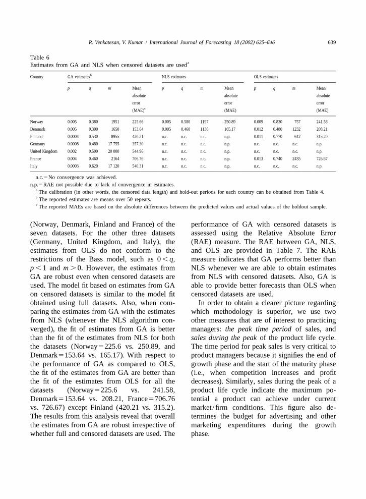
(Norway, Denmark, Finland and France) of the performance of GA with censored datasets isseven datasets. For the other three datasets assessed using the Relative Absolute Error(Germany, United Kingdom, and Italy), the (RAE) measure. The RAE between GA, NLS,estimates from OLS do not conform to the and OLS are provided in Table 7. The RAErestrictions of the Bass model, such as 0, q, measure indicates that GA performs better thanp ,1 and m . 0. However, the estimates from NLS whenever we are able to obtain estimatesGA are robust even when censored datasets are from NLS with censored datasets. Also, GA isused. The model fit based on estimates from GA able to provide better forecasts than OLS whenon censored datasets is similar to the model fit censored datasets are used.obtained using full datasets. Also, when com- In order to obtain a clearer picture regardingparing the estimates from GA with the estimates which methodology is superior, we use twofrom NLS (whenever the NLS algorithm con- other measures that are of interest to practicingverged), the fit of estimates from GA is better managers:the peak time period of sales, andthan the fit of the estimates from NLS for both sales during the peak of the product life cycle.the datasets (Norway5225.6 vs. 250.89, and The time period for peak sales is very critical toDenmark5153.64 vs. 165.17). With respect to product managers because it signifies the end ofthe performance of GA as compared to OLS, growth phase and the start of the maturity phasethe fit of the estimates from GA are better than (i.e., when competition increases and profitthe fit of the estimates from OLS for all the decreases). Similarly, sales during the peak of adatasets (Norway5225.6 vs. 241.58, product life cycle indicate the maximum po-Denmark5153.64 vs. 208.21, France5706.76 tential a product can achieve under currentvs. 726.67) except Finland (420.21 vs. 315.2). market /firm conditions. This figure also de-The results from this analysis reveal that overall termines the budget for advertising and otherthe estimates from GA are robust irrespective of marketing expenditures during the growthwhether full and censored datasets are used. The phase.
640 R. Venkatesan, V. Kumar / International Journal of Forecasting 18 (2002) 625–646
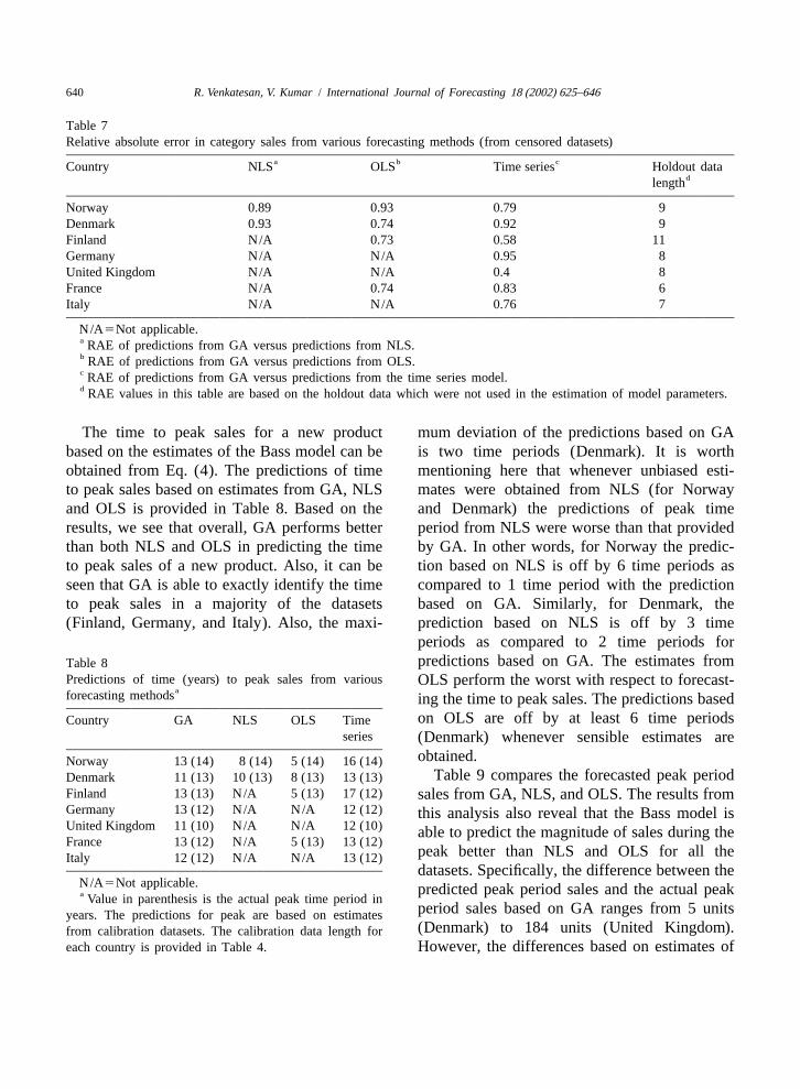
Table 7Relative absolute error in category sales from various forecasting methods (from censored datasets)
a b cCountry NLS OLS Time series Holdout datadlength
Norway 0.89 0.93 0.79 9Denmark 0.93 0.74 0.92 9Finland N/A 0.73 0.58 11Germany N/A N/A 0.95 8United Kingdom N/A N/A 0.4 8France N/A 0.74 0.83 6Italy N/A N/A 0.76 7
N/A5Not applicable.a RAE of predictions from GA versus predictions from NLS.b RAE of predictions from GA versus predictions from OLS.c RAE of predictions from GA versus predictions from the time series model.d RAE values in this table are based on the holdout data which were not used in the estimation of model parameters.
The time to peak sales for a new product mum deviation of the predictions based on GAbased on the estimates of the Bass model can be is two time periods (Denmark). It is worthobtained from Eq. (4). The predictions of time mentioning here that whenever unbiased esti-to peak sales based on estimates from GA, NLS mates were obtained from NLS (for Norwayand OLS is provided in Table 8. Based on the and Denmark) the predictions of peak timeresults, we see that overall, GA performs better period from NLS were worse than that providedthan both NLS and OLS in predicting the time by GA. In other words, for Norway the predic-to peak sales of a new product. Also, it can be tion based on NLS is off by 6 time periods asseen that GA is able to exactly identify the time compared to 1 time period with the predictionto peak sales in a majority of the datasets based on GA. Similarly, for Denmark, the(Finland, Germany, and Italy). Also, the maxi- prediction based on NLS is off by 3 time
periods as compared to 2 time periods forpredictions based on GA. The estimates fromTable 8
Predictions of time (years) to peak sales from various OLS perform the worst with respect to forecast-aforecasting methods ing the time to peak sales. The predictions based
on OLS are off by at least 6 time periodsCountry GA NLS OLS Timeseries (Denmark) whenever sensible estimates are
obtained.Norway 13 (14) 8 (14) 5 (14) 16 (14)Table 9 compares the forecasted peak periodDenmark 11 (13) 10 (13) 8 (13) 13 (13)
Finland 13 (13) N/A 5 (13) 17 (12) sales from GA, NLS, and OLS. The results fromGermany 13 (12) N/A N/A 12 (12) this analysis also reveal that the Bass model isUnited Kingdom 11 (10) N/A N/A 12 (10) able to predict the magnitude of sales during theFrance 13 (12) N/A 5 (13) 13 (12)
peak better than NLS and OLS for all theItaly 12 (12) N/A N/A 13 (12)datasets. Specifically, the difference between the
N/A5Not applicable. predicted peak period sales and the actual peaka Value in parenthesis is the actual peak time period inperiod sales based on GA ranges from 5 unitsyears. The predictions for peak are based on estimates(Denmark) to 184 units (United Kingdom).from calibration datasets. The calibration data length for
each country is provided in Table 4. However, the differences based on estimates of
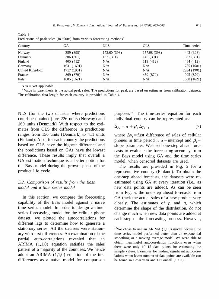
R. Venkatesan, V. Kumar / International Journal of Forecasting 18 (2002) 625–646 641
Table 9aPredictions of peak sales (in ’000s) from various forecasting methods
Country GA NLS OLS Time series
Norway 359 (398) 172.60 (398) 157.98 (398) 443 (398)Denmark 306 (301) 132 (301) 145 (301) 337 (301)Finland 405 (412) N/A 119 (412) 484 (412)Germany 1631 (1601) N/A N/A 1785 (1601)United Kingdom 1717 (1901) N/A N/A 2334 (1901)France 869 (870) N/A 459 (870) 995 (870)Italy 1685 (1621) N/A N/A 1688 (1621)
N/A5Not applicable.a Value in parenthesis is the actual peak sales. The predictions for peak are based on estimates from calibration datasets.
The calibration data length for each country is provided in Table 4.
10NLS (for the two datasets where predictions purposes . The time-series equation for eachcould be obtained) are 226 units (Norway) and individual country can be represented as:169 units (Denmark). With respect to the esti-
Dy 5a 1b Dy (7)t 1 t21mates from OLS the difference in predictionsranges from 156 units (Denmark) to 411 units whereDy 5first difference of sales of cellulari(Finland). Also, for each country the predictions phones in time periodi, a5intercept andb 5sbased on OLS have the highest difference and slope parameter. We used one-step ahead fore-the predictions based on GAs have the lowest casts to evaluate the forecasting accuracy fromdifference. These results imply that overall a the Bass model using GA and the time seriesGA estimation technique is a better option for model, when censored datasets are used.the Bass model during the growth phase of the The results are provided in Fig. 5 for aproduct life cycle. representative country (Finland). To obtain the
one-step ahead forecasts, the datasets were re-estimated using GA at every iteration (i.e., as5 .2. Comparison of results from the Bassnew data points are added). As can be seenmodel and a time series modelfrom Fig. 5, the one-step ahead forecasts from
In this section, we compare the forecasting GA track the actual sales of a new product very¨capability of the Bass model against a naıve closely. The estimates ofp and q, which
time series model. In order to design a time- determine the shape of the distribution, do notseries forecasting model for the cellular phone change much when new data points are added atdataset, we plotted the autocorrelations for each step of the forecasting process. However,different lags to determine how to generate a
10stationary series. All the datasets were station- We chose to use an ARIMA (1,1,0) model because thetime series model performed better than an exponentialary with first differences. An examination of thesmoothing or a moving average model. We were able topartial auto-correlations revealed that anobtain meaningful autocorrelation functions even whenARIMA (1,1,0) equation satisfies the salesthere were only 10–15 data points for estimating the
pattern of a majority of the countries. We hence sample values. Examples for finding significant autocorre-adopt an ARIMA (1,1,0) equation of the first lations when lesser number of data points are available can
¨differences as a naıve model for comparison be found in Bowerman and O’Connell (1993).

642 R. Venkatesan, V. Kumar / International Journal of Forecasting 18 (2002) 625–646
Fig. 5. One step ahead forecasts for Finland.
the value of the estimate ofm does change maximum deviation based on predictions fromwhen new data points are added. The above GA is two time periods (Denmark) as comparedpattern is intuitive given thatp andq determine to five time periods (Norway) for predictionsthe shape of the diffusion curve, and hence need from the time series model. Finally, while the
¨not change with additional information after the naıve time series model performs better thaninflection point is reached. However, the value NLS and OLS with respect to predicting theof m provides magnitude to the diffusion curve, magnitude of peak sales it does not compareand the short-term one step ahead forecasts will well with the Bass model estimated using GA.depend on the value ofm. It can be inferred Specifically, the difference in predicted peakfrom Fig. 5 that GA is very useful to managers sales and actual peak sales based on the timeto generate short-term one-step ahead forecasts series model is consistently higher than theof sales and long-term forecasts regarding the respective difference based on the predictionsshape of the curve. from GA. In summary, the Bass model esti-
The Bass model estimated using GA also mated using GA is clearly the best option when¨fares better than a naıve time series model with long range forecasting is the requirement. For
respect to one-step ahead forecasts. The RAE short-term forecasts, researchers should investi-for the Bass model versus the time series model gate the utility of a combination of forecasts
¨is lower (less than one) for all the countries from the Bass model and a naıve time seriesanalyzed (as shown in Table 7). However, the model.

R. Venkatesan, V. Kumar / International Journal of Forecasting 18 (2002) 625–646 643
Fig. 6. Forecasts for years 2000 and 2001.

644 R. Venkatesan, V. Kumar / International Journal of Forecasting 18 (2002) 625–646
5 .2.1. Future forecasts market is a long-term phenomenon. The fore-In this section we provide forecasts of future casts based on GA suggest that the sales of
sales of cellular phones (over a two year cellular phones are (1) expected to grow only inhorizon) in the seven countries studied. The Norway, (2) the sales have reached a stationaryresults of this forecasting exercise are provided state in Finland and Denmark, and (3) the salesin Fig. 6. As indicated in Fig. 6a, the sales of is expected to slowdown in France, UK, Italy,cellular phones seem to have stabilized for and Germany. The results indicate that overallFinland and Denmark. The prospects for growth the growth rate for cellular phones is reachingare high only for Norway, while the sales of maturity and that firms should focus on newercellular phones are predicted to decline for and useful innovations if they need to sustainGermany, UK, Italy, and Denmark. Overall, the their current growth rate and profit margins.telecommunications industry seems to have The forecast of wireless subscribers in ourstabilized and high growth rates as observed in study was accomplished by estimating thethe past may not be experienced in the future. Srinivasan and Mason (1986) operationalizationAlso, there doesn’t seem to be any drastic of the Bass diffusion model using GA. Thechanges in the diffusion trend for the future results from our analyses using GA are verysales. The results of our analyses also imply that encouraging to both practitioners and research-the forecasts of sustained growth in the tele- ers alike. It is found that the predictions fromcommunications industry need to be qualified. GA are robust across many datasets and are
better than OLS and NLS with respect to bothRelative Absolute Error (RAE) and predictionsof time to peak sales, when forecasting is done6 . Conclusions and future researchin the growth phase and the maturity phase of
In this study we address the issue of forecast- product life cycle. The Bass model estimated¨ing sales in dynamic and turbulent markets such using GA also performed better than a naıve
as the telecommunications sector. Specifically time series model (Eq. (7)). The estimatesduring the growth phase, volatility with respect generated from a GA also have desirable prop-to price, new product offerings and competitor erties such as (1) a normal distribution and (2)actions, and entry of new brands (as evident in bounded variance.the telecommunication sector) make predicting Future research studies can investigate thefuture sales, time to peak sales and magnitude utility of including several exogenous factorsof peak sales a non-trivial task for product such as price, competitive intensity, and net-managers. The current slowdown in growth in work effects in obtaining better predictionsthe telecommunications sector makes such a during the growth phase. The recent phase ofstudy of critical importance. In order to achieve consolidation in the telecommunications indus-this objective we propose a simulation based try could provide avenues to investigate how thesearch technique for estimating the Bass model competitive intensity, measured in terms ofand illustrate our algorithm by providing predic- market share concentration or price volatility,tions of category sales, time of peak sales, and influences the diffusion of new products andsales at the peak, of cellular phones in seven telecommunications equipment in particular.countries during the growth phase of its life Also, the telecommunication industry is depen-cycle. The results suggest that in the seven dent to a large extent on network externalitiesEuropean countries in our study the current such as high bandwidth for better communica-slowdown in growth in the wireless phones tion facilities and hence higher rates and levels

R. Venkatesan, V. Kumar / International Journal of Forecasting 18 (2002) 625–646 645
Bass Model fits without decision variables.Marketingof adoption. The above examples illustrate someScience, 3, 203–223.representative theoretical and managerial issues
Bayus, B. L. (1992). The dynamic pricing of next gene-that need to be resolved in the telecommunica- ration consumer durables.Marketing Science, 11(3),tions sector related to product /service adoption. 251–266.The technique proposed in this study can be Bowerman, B. L., & O’Connell, R. T. (1993).Forecasting
and Time Series: An Applied Approach, 3rd ed.. Bel-used as a basis for further investigation ofmont, California: DuxBury Press.product adoption in nascent markets. Research-
Fildes, R. (2002). Telecommunications demand forecast-ers should also investigate the applicability ofing—a review. International Journal of Forecasting,
these results across different product categories, 18.especially those that have different product Ganesh, J., Kumar,V., & Subramanian,V. (1997). Learningmarket characteristics such as High Definition effect in multinational diffusion of consumer durables:
an exploratory investigation.Journal of the Academy ofTelevisions. In this study, we investigate onlyMarketing Science., 25(3), 214–228.one aspect of the drawbacks in using NLS for
Goldberg, D. E. (1989). InA Simple Genetic Algorithm inestimating the Bass model. The issue of sys-Genetic Algorithms in Search Optimization and Ma-
tematic change and bias in parameter estimates chine Learning. Addison Wesley Longman, pp. 10–14.of the Bass model when using NLS still needs Griffiths, W. E., Hill, R. C., & Judge, G. G. (1993).
Learning and Practicing Econometrics. New York: Johnto be investigated. GAs could very well serve asWiley & Sons.an alternative estimation technique under this
Hyman, M. R. (1988). The timeliness problem in thescenario.application of Bass-type new product growth models to
Of primary interest however, would be to durable sales forecasting.Journal of Business Research,investigate the performance of GAs compared 16(1), 31–47.to newer techniques such as Hierarchical Bayes,Jamieson, L. F., & Bass, F. M. (1989). Adjusting stated
intention measures to predict trial purchase.Journal ofKalman filtering, and any combinations of theseMarketing Research, 26(3), 336–346.methods. Also, research is needed on deriving
Jain, D. C., & Rao, R. C. (1990). Effect of price on thealgorithms to combine the forecasts from these demand for durables: modeling, estimation, and find-different techniques. ings. Journal of Business and Economic Statistics, 8,
163–170.Kumar, V., & Krishnan, T. V. (2002). Multinational diffu-
sion models: an alternative framework for modelingA cknowledgementscross-national diffusion.Marketing Science, 21(3),318–330.
The authors thank the editor-in-chief, the Lawrence, K. D., & Lawton, W. H. (1981). Application ofreviewers, Frank M. Bass, Trichy V. Krishnan, diffusion models: some empirical results. In Wind, Y.,Robert P. Leone, and Srini Srinivasan for their Mahajan, V., & Cardozo, R. C. (Eds.),New Product
Forecasting. Lexington, MA: Lexington Books, pp.comments on earlier versions of this paper.529–541.
Lenk, P. J., & Rao, A. G. (1990). New models from oldforecasting product adoption by hierarchical Bayes
R eferences procedures.Marketing Science, 9, 42–53.Mahajan, V., Muller, E., & Bass, F. M. (1990). New
Bass, F. M. (1969). A new product growth model for product diffusion models in marketing in: a review andconsumer durables.Management Science, 15, 215–227. directions for future research.Journal of Marketing,
Bass, F. M. (1980). The relationship between diffusion 54(1), 1–26.rates, experience curves, and demand elasticities for Mahajan, V., & Sharma, S. (1986). A simple algebraicconsumer durable technological innovations.Journal of estimation procedure for innovation diffusion models ofBusiness, 53, 51–67. new product acceptance.Technological Forecasting and
Bass, F. M., Krishnan, T. V., & Jain, D. (1994). Why the Social Change, 30, 331–345.

646 R. Venkatesan, V. Kumar / International Journal of Forecasting 18 (2002) 625–646
Meade, N., & Islam, T. (2001). Forecasting the diffusion Biographies: V. KUMAR (VK) is the ING Chairof innovations for time-series extrapolation. In Am- Professor of Marketing, and Executive Director, INGstrong, S. (Ed.),Principles of Forecasting: A Handbook Center for Financial Services in the School of Business,for Researchers and Practitioners. Boston: Kluwer University of Connecticut. He has been recognized withAcademic Publishers, pp. 577–596. many teaching and research excellence awards and has
Modis, T., & Debecker, D. (1992). Chaoslike states can be published numerous articles in many scholarly journals inexpected before and after logistic growth.Technological marketing including theHarvard Business Review, JournalForecasting and Social Change, 41, 111–120. of Marketing, Journal of Marketing Research, Marketing
Kalish, S. (1983). Monopolistic pricing with dynamic Science, and Operations Research. He has co-authoreddemand and production cost.Marketing Science, 2, multiple textbooks onMarketing Research. His interest in135–160. International and Forecasting area is very well reflected by
Kotler, P. (2000).Marketing Management. Prentice Hall. his research publications in many major journals includingKrishnan, T. V., Bass, F. M., & Kumar, V. (2000). Impact theInternational Journal of Forecasting, Journal of
of a late entrant on the diffusion of a new product or International Marketing, International Journal of Re-service.Journal of Marketing Research, 269–278. search in Marketing, and theJournal of World Business.
Kumar, V., Ganesh, J., & Echambadi, R. (1998). Cross- He has authored a book titledInternational Marketingnational diffusion research: what do we know and how Research, which is based on his marketing researchcertain are we?Journal of Product Innovation Manage- experience across the globe. He is on the editorial reviewment, 15, 225–268. board of many scholarly journals and has lectured on
Parker, Philip M. (1994). Aggregate diffusion forecasting marketing-related topics in various universities and organi-models in marketing: a critical review.International zations worldwide. His current research focuses on interna-Journal of Forecasting, 10, 353–381. tional diffusion models, customer relationship manage-
Robinson, B., & Lakhani, C. (1975). Dynamic price ment, customer lifetime value analysis, sales and marketmodels for new product planning.Management Science, share forecasting, international marketing research and10, 1113–1122. strategy, coupon promotions, and market orientation. He
Schmittlein, D. C., & Mahajan, V. (1982). A maximum served on the Academic Council of the AMA as a Seniorlikelihood estimation for an innovation diffusion model V.P. for Conferences and Research and a Senior V.P. forof new product acceptance.Marketing Science, 1, 57– International Activities. He was recently listed as one of78. the top fifteen scholars in marketing worldwide. He is a
Seber, G. A. F., & Wild, C. J. (1993).Nonlinear Regres- consultant for many Fortune 500 firms and has alsosion. New York: John Wiley. worked with these companies’ databases to identify profit-
Srinivasan, V., & Mason, C. H. (1986). Nonlinear least able customers. He received his Ph.D. from the Universitysquares estimation of new product diffusion models. of Texas at Austin.Marketing Science, 5(2), 169–178.
Sultan, F., Farley, J. U., & Lehnmann, D. R. (1990). Ameta-analysis of diffusion models.Journal of MarketingResearch, 27, 70–77. Rajkumar VENKATESAN is Assistant Professor of
Takada, H., & Jain, D. C. (1991). Cross-national analysis Marketing at the University of Connecticut. He has aof diffusion of consumer durable goods in Pacific Rim Bachelors degree in Computer Science and Engineeringcountries.Journal of Marketing, 55, 48–54. from University of Madras. Raj’s research interests include
Van den Bulte, C., & Lilien, G. L. (1997). Bias and Customer Relationship Management, Customer equity vs.systematic change in the parameter estimates of macro firm value, E-Business models, and new product innova-level diffusion models. Marketing Science, 16(70), tions. He is the winner of the2001 Alden G. Clayton338–353. Dissertation Proposal award from the Marketing Science
Venkatesan, R., Krishnan, T.V., & Kumar, V. (2001). Institute, the 2001ISBM Doctoral Dissertation competitionStructural Asymmetry and Consistent Estimation of Outstanding Submission award and theBest Track PaperMacro-level Diffusion Models. Working Paper, Uni- Award in the 1999 American Marketing Associationversity of Connecticut. Winter Marketing Educator’s Conference.