A generalized longitudinal mixture IRT model for measuringdifferential growth in learning environments

Damazo T. Kadengye & Eva Ceulemans &

Wim Van den Noortgate

Published online: 21 November 2013# Psychonomic Society, Inc. 2013

Abstract This article describes a generalized longitudinalmixture item response theory (IRT) model that allows fordetecting latent group differences in item response data ob-tained from electronic learning (e-learning) environments orother learning environments that result in large numbers ofitems. The describedmodel can be viewed as a combination ofa longitudinal Rasch model, a mixture Rasch model, and arandom-item IRT model, and it includes some features of theexplanatory IRT modeling framework. The model assumesthe possible presence of latent classes in item response pat-terns, due to initial person-level differences before learningtakes place, to latent class-specific learning trajectories, or to acombination of both. Moreover, it allows for differential itemfunctioning over the classes. A Bayesian model estimationprocedure is described, and the results of a simulation studyare presented that indicate that the parameters are recoveredwell, particularly for conditions with large item sample sizes.The model is also illustrated with an empirical sample data setfrom a Web-based e-learning environment.

Keywords Item response theory . E-learning .Modeling ofgrowth .Mixture models

Longitudinal item response theory (IRT) models (Andersen,1985; Andrade & Tavares, 2005; Embretson, 1991; Fischer,1989; Paek, Baek, & Wilson, 2012; Roberts & Ma, 2006; vonDavier, Xu, & Carstensen, 2009) can be used to measureindividual differences in growth (or change) over time. Mea-surement of growth in student performance between two ormore testing occasions is a central topic in educational researchand assessment (Fischer, 1995). In educational learning envi-ronments, such longitudinal IRT models can be interesting forresearchers whose interest is in tracking and monitoring per-sons’ progress over time in response to a treatment such asteaching or training (Miceli, Settanni, & Vidotto, 2008). This isthe case in studies in which students are followed from onegrade to another over a period of time in such a way that, everyacademic year, students are subjected to a set of differenttests—for instance, at the beginning of the term and at midterm,end of term, and end of year. In this way, educators can evaluatethe effectiveness of their employed training procedures, so thatthey may be in position to make more informed instructionaldecisions (Safer & Fleischman, 2005).

Modeling growth in individuals

One approach for modeling growth over time is the use of themultidimensional Rasch model of Andersen (1985) or that ofEmbretson (1991), which can be employed when the same orseparate sets of items are repeatedly answered by a group ofpersons over different measurement occasions in time. Forinstance, Embretson’s multidimensional Rasch model forlearning and change assumes the involvement of M abilitiesin item responses within K measurement occasions, such that(a) on the first measurement occasion (k = 1) only an initialability (θp1) is involved in the item responses of person p , and(b) on the later k > 1 occasions, that ability (θp1) plus k − 1additional abilities are involved in the performance.

D. T. Kadengye :W. Van den NoortgateFaculty of Psychology and Educational Sciences and ITEC–iMinds,University of Leuven–Kulak, Kortrijk, Belgium

D. T. Kadengye : E. Ceulemans :W. Van den NoortgateCentre for Methodology of Educational Research, University ofLeuven, Leuven, Belgium

D. T. Kadengye (*)Faculty of Psychology and Educational Sciences, KU Leuven–Kulak, Etienne Sabbelaan 53, 8500 Kortrijk, Belgiume-mail: dkadengye@gmail.com

Behav Res (2014) 46:823–840DOI 10.3758/s13428-013-0413-3

Embretson’s model can be expressed as

P Ypik ¼ 1 θ�p1; θ�p2;…; θ�pk

� ���� ;βi

� �¼ exp

Xm¼1

k

θ�pm−βi

!.

1þ expXm¼1

k

θ�pm−βi

!; ð1Þ

where θp1* =θp1 is the baseline level (Occasion 1) ability for

person p (p =1,2,…,P ), θpk* =θpk−θp(k−1) is the change in

ability for person p from occasion k − 1 to occasion k (fork =2,…,K ) and πpik=Prob(Ypik=1|θpk,β i) is the probability

that person p with ability θpk ¼ ∑m¼1k

θ�pm at occasion k willanswer item i (i =1,2,…,I) with difficulty β i correctly on thatparticular occasion. The θs are assumed to be multivariate andnormally distributed over persons, whereas the item difficultyparameters, β i, are assumed to be the same for all occasions.Note that only I − 1 item difficulties can be estimated fromEq. 1, unless the intercept is constrained to be zero (otherwise,the model is not identified).

Equation 1, as with other common IRT models, can beregarded as a logistic mixed model (Kamata, 2001). Further-more, instead of assuming unknown, fixed values of the itemdifficulties (as in Eq. 1), the considered items can also beregarded as a random sample from a population of items andtherefore item difficulties can also be modeled as randomeffects over items (De Boeck, 2008; De Boeck & Wilson,2004; Van Den Noortgate, De Boeck, & Meulders, 2003). Assuch, the item difficulties are assumed to be randomly andnormally distributed over items but constant over occasions.In this way, Eq. 1 can be simplified to a generalized linearmixed model (GLMM) with crossed random effects, as

logit πpik

� � ¼ b0 þXk¼2

K

bkDpik þXk¼1

K

ωpkDpik þ υi; ð2Þ

where b 0 is the expected initial person ability, bk is thedifference from b0 at occasion k such that the expected overallability at occasion k is b0+bk, and Dpik is a dummy variableequal to 1 if item i was solved by person p at session k , or 0otherwise. The variable ωpk is the random deviation of theability of person p from the overall ability at occasion k , thatcan be assumed multivariate normal N(0 ,Σ*) over personswith Σ* as the variance–covariance matrix. In this case, theability estimate of person p during occasion k , θpk in Eq. 1, isnow given by b0+bk+ωpk. The υ is are random item param-eters with υ i∼N(0,συ

2), where υ i corresponds to −β i of Eq. 1,and therefore cannot be interpreted as the item difficulty, butrather as the item easiness.

Measuring growth in e-learning environments

A specific application is in electronic learning (e-learning)environments in which persons can freely engage items onlineas part of formal education to build and improve their ability(for examples, see Desmet, Paulussen, & Wylin, 2006;Klinkenberg, Straatemeier, & Van der Maas, 2011). For eachengaged item, an individual gets instant feedback (e.g., aboutthe correctness of the answer) to enhance learning. On the basisof the time points at which the items are engaged, we can definefor each person one or more study sessions. For instance, if oneday minimally separates answering two items, we could con-clude that the person has started a new study session (see, e.g.,Cepeda, Vul, Rohrer, Wixted, & Pashler, 2008; Vlach &Sandhofer, 2012). If we consider responses to items that areengaged in the same study session as being solved at onemeasurement occasion, Eq. 2 can be employed to track per-sons’ growth from one study session to another. In this case,items need not be the same for all sessions, or for each person,provided that not all items solved at a specific occasion aresolved at that occasion only, so that scales are still linked acrosssessions and across persons. This requirement is even notnecessary if item difficulties can already be considered asknown—for instance, on the basis of a prior calibration study.

In some e-learning environments, the total number of avail-able items can be very large, but the number of items per studysession small. For instance, the item bank of the Math Gardene-learning environment (Klinkenberg et al., 2011) consists of 2,784 items. Yet, each study session corresponds to 15 items only.Such a scenario can lead to many study sessions such that, ifEq. 2 is employed to the data, the number of parameters toestimate can be very large, thereby limiting easy interpretationof the results. Moreover, due to user freedom, the number ofitems per session over persons is likely to vary greatly, as wellas the space between study sessions. This further makes Eq. 2less suitable for comparisons of individuals from one studysession to another. Instead, we can use session as a continuouspredictor variable and, for instance, define a person’s ability aslinearly changing over study sessions. In this way, the GLMMin Eq. 2 can be rewritten as

logit πpik

� � ¼ b0 þ ω0p

� �þ b1 þ ω1p

� �sessionpk þ υi; ð3Þ

where Ypik is equal to 1 if person p answers item i correctlyduring the k th session, Ypik∼binomial(1,πpik), and sessionpkis the k th study session of person p . Therefore, b0 is theexpected initial ability, b1 is the overall population slope inperson abilities for the sessions, ω0p is the random deviationof person p from the overall initial ability b0, ω1p is therandom deviation of person p from the overall slope b1 oversessions, and υ i is the random item easiness parameter, as inEq. 2. The population distribution of the two random person-specific effects (ω0p,ω1p) can be assumed to be multivariate

824 Behav Res (2014) 46:823–840

normalN (0 ,Σ ) over persons, withΣ as the variance–covari-ance matrix. The parameters that are estimated are the meaninitial ability and growth slope, b0 and b1, as well as the(co)variances of the random effects, συ

2 and Σ . The value ofb0+ω0p+(b1+ω1p)sessionpk corresponds to θpk, the abilityof person p during session k . The linear growth assumption isconsidered here for simplicity of explanation purposes, but inpractice other growth assumptions, such as quadratic or expo-nential, can be considered.

In situations in which the interest is in monitoring growth forobserved groups of persons rather than in focusing on the wholepopulation of individuals, indicator variables for manifest persongroups like gender, course of study, or ethnicity can be includedas predictors in Eq. 3 (for examples, see Cho, Athay, & Preacher,2013; Rost, 1990). This is similar to the explanatory IRTmodel-ing framework of De Boeck and Wilson (2004), inwhich IRT models are formulated as GLMMs. Inclusionof manifest person groups as predictors offers flexibleways for predicting and understanding differences inability and preferences (of groups) of persons. For in-stance, if persons are classified in two or more groups, includ-ing in Eq. 3 a set of dummy indicators for group membershipand their interactions with the session number would provideparameter estimates for group-specific growth trends. Further-more, interaction terms of person groups by item indicatorscan be included in the model to assess the presence of differ-ential item functioning (DIF), as was demonstrated by VanDen Noortgate and De Boeck (2005). A heteroscedastic ex-planatory IRT model further allows person random effects’variance to be different for the manifest groups’ levels.

Including person group indicators is only possible wheninformation on groups has been recorded during data collec-tion. However, information on some sensitive person proper-ties, such as gender or ethnicity, is often not readily available ine-learning environments, due to user independence and free-dom, design, or nonresponse. Even when group information isavailable, Samuelsen (2008) has argued that manifest charac-teristics can be poor proxies in certain situations for latentgroups such as educationally advantaged or disadvantagedstudents. Rather, it is more common that persons belonging tothe same manifest group will belong to different latent classes,because the set of characteristics that is the root of the latentclass formation is not exactly the same as that of the manifestgroup formation (Bilir, 2009). In such situations, understandingthe reasons behind differential performance can be difficult(Bilir, 2009; Dai & Mislevy, 2009; Samuelsen, 2008).

Such unobserved heterogeneity can be addressed by mix-ture IRT models, which infer latent groups from the data (Cho& Cohen, 2010). The mixture IRT models that are employedin most research studies are generic extensions of Rost’s(1990) mixture Raschmodel, which assumes that a populationof persons is composed of a fixed number of exhaustive andmutually exclusive latent classes. In the mixture Rasch model,

the logit of the probability of a correct response by person pfrom class g on item i can be given as

logit πpig

� � ¼ b0g þ ωpg þ υig andYpig∼binomial 1;πpig

� �;ð4Þ

where g =1,2,…,G is an index for mutually exclusive latentclasses, b0g is the expected initial ability for class g , ωpg is therandom deviation of person p in class g from b0g—the overallinitial ability of class g—and υ ig is the easiness parameter ofitem i for class g . The structure of the ability in Eq. 4 is suchthat ωpg∼N (0,σg

2), where σg2 is the class-specific variance of

ability. Within each latent class, the model described in Eq. 4is assumed to hold, but each class may have different itemeasiness parameters and another distribution of person abilityparameters, although the model can be simplified byconstraining some parameters to be the same over classes.

Mixture IRT models have been widely used in educationalscience and psychology. They have, for instance, been appliedto investigating individual differences in the selection of re-sponse categories in multiple-choice items of a college-levelEnglish placement test (Bolt, Cohen, & Wollack, 2001); fordetecting latent groups of persons for whom items functiondifferently (Cohen & Bolt, 2005; Mislevy & Verhelst, 1990);for identifying latent subgroups of adolescents on the basis oftheir propensity to engage in sexually and substance use riskybehaviors (Finch & Pierson, 2011); and for describing DIF atboth the school and student levels for a standardized mathemat-ics test in a multilevel setting (Cho & Cohen, 2010). In therecent past, mixture IRT models have started to gain consider-able attention in longitudinal IRTmodels for measuring change,specifically those for understanding and explaining differentialgrowth as a result of learning or training in educational envi-ronments (cf. Cho, Bottge, Cohen, & Kim, 2011; Cho, Cohen,& Bottge, 2013; Cho, Cohen, Kim, & Bottge, 2010).

This study extends on this growing research domain oflongitudinal mixture IRT modeling, but focuses mainly ondata sets from Web-based e-learning environments. Specifi-cally, we incorporate the growth trend of Eq. 3 into themixture IRT model of Eq. 4 in order to estimate differentiallatent growth that might be present in data sets from e-learningenvironments. The resulting generalized longitudinal mixtureIRT model can be used to detect and compare latent classes inthe data as a result of latent differential growth trends or otherunobserved characteristics. We expected that this model willprovide possibilities for estimates of growth trends specific tounobserved groups in a population of persons, as compared tothe longitudinal model in Eq. 3, which provides estimates forthe whole population. The remainder of the article will beorganized as follows: First, the generalized longitudinal mix-ture IRT model is formulated, followed by a brief discussionon the estimation of model parameters. Next, a simulationstudy design used to evaluate the model is described. Theobtained results are then discussed by focusing on the ability

Behav Res (2014) 46:823–840 825

of the presented model to recover the simulated parametersand the correct classification of participants under differentconditions. The proposed model is then applied to an empir-ical example, and finally, a brief discussion is given.

The generalized longitudinal mixture IRT model

The proposed generalized longitudinal mixture IRT modelallows for a mixture of latent classes of persons that differ fromeach other in two different aspects. First, the proposed modelassumes that response patterns may be heterogeneous overclasses due to initial person-level differences (Mislevy &Verhelst, 1990; Rost, 1990). This can, for instance, be the casein situations in which the random person ability values areheterogeneous, with persons belonging to one class assumedto have, on average, higher abilities than their counterparts inother classes before learning takes place. Furthermore, theproposed model assumes that growth trends over time can alsobe heterogeneous, with persons in one class tending to have, onaverage, higher growth trends than those in other classes. Thiscan happen, for instance, when one group of persons is moremotivated to learn or solve items than the other, or when onegroup has better learning strategies than the other. The model,however, does not exclude the possibility that there may be noinitial differences between latent person classes, but only class-specific growth trends, and vice versa. This is because the utilityof mixture IRT modeling approach lies in the fact that latentclasses, although not immediately observable, are defined bycertain shared response patterns that can be used to help explainitem-level performance about how the members of one latentclass differ from those of another (Cho & Cohen, 2010).

In this regard, the probability of getting a correct score inthe generalized mixture longitudinal IRT model can be ob-tained from Eqs. 3 and 4 as follows:

logit πpigk

� � ¼ b0g þ b1g þ ω1pg

� �sessionpgk þ ω0pg þ υig; ð5Þ

where b0g and b1g are defined as before, but each is nowspecific to latent class g ; ω0pg and ω1pg are the respectiveclass-specific random deviations for initial ability and thesessions’ slopes, assumed to be distributed with ω 0pg∼N(0,σω0g

2 ) and ω1pg∼N(0,σω1g2 ); and υ ig is the random effect

for item i within class g , with class-specific distributionassumptions such that υ ig∼N (0,συg

2 ). In this model, eachperson is parameterized by a class-specific parameter, suchthat the ability parameter for person p in any given studysession is given by θpgk=b0g+ω0pg+(b1g+ω1pg)sessionpgk.For each latent class, the item easiness values υ ig can beobtained and investigated further. When some of the itemeasiness values are different across the latent classes, this isconsidered as DIF.

From Eqs. 4 and 5, if, for instance, one has two classes and adummy indicator for each class is added, one cannot estimate acommon intercept anymore; rather, class-specific intercepts areobtained. Similarly, for Eq. 5, if interaction terms betweensession and the two dummies are included, one can not includethe main effect of session anymore to allow for model identi-fication. The model in Eq. 5 can be looked at as belonging tothe family of the GLMMs described by De Boeck and Wilson(2004), or to the generalized linear latent and mixed models(GLLAMM; cf. Rabe-Hesketh, Skrondal, & Pickles, 2004a),since both an item response model and a mixture model areexpressed simultaneously in it. The specificity of this model liesin the incorporation of the learning trends and the fact that thesetrends can be specific to unobserved discrete classes. Onceobtained, relations with external variables can be identified inorder to understand what the different latent classes are.

Parameter estimation

The parameters of the generalized longitudinal mixture IRTmodel can be estimated using Bayesian inference via theMarkov-chain Monte Carlo (MCMC) estimation algorithm inWinBUGS (Lunn, Thomas, Best, & Spiegelhalter, 2000).MCMC estimation algorithms are receiving increasing attentionin mixture IRT models (see, e.g., Bilir, 2009; Bolt et al., 2001;Cho & Cohen, 2010; Cohen & Bolt, 2005; Dai & Mislevy,2009; Frederickx, Tuerlinckx, De Boeck, & Magis, 2010). InMCMC estimation, a Markov chain is simulated in whichvalues representing parameters of the model are repeatedlysampled from their full conditional posterior distributions overa large number of iterations. To derive the posterior distributionsfor each parameter in amixture IRTmodel, it is first necessary tospecify their prior distributions (Cohen & Bolt, 2005). Theposterior distribution of the parameters of interest Ω , given theobserved data Y, is then obtained using Bayes’s theorem:

P Ω Yjð Þ ¼ P Ωð ÞP Y Ωjð ÞP Yð Þ ð6Þ

where P(Ω ) is the prior density for Ω , P(Y |Ω ) is the condi-tional probability ofY givenΩ , andP(Y) is themarginal densityof the observed dataY. The posterior of themodel parameters arecomputed fromEq. 6, whose integral is typically evaluated usingMonte Carlo integration techniques. For a detailed discussion ofthe MCMC estimation algorithm for mixture IRT models, inter-ested readers are referred to Bolt et al. (2001).

Typically, vague or noninformative priors are used forparameters about which not much is known beforehand(Frederickx et al., 2010), but this may not always work outwell in practice. In fact, Bilir (2009) and Cho and Cohen(2010) noted that noninformative priors tend to fail in provid-ing enough bounds for the parameter estimates of a mixtureIRT model. Various prior choices for the parameters,

826 Behav Res (2014) 46:823–840

especially those for the standard deviation components inrandom-effects models, have been proposed in the Bayesianliterature, with no standard solution (Frederickx et al., 2010).In general, however, one considers all parameters of the modelto be random variables, and mildly informative priors thatprovide more stable fitting procedures for the model parame-ters and hyperparameters can be applied (Cho&Cohen, 2010;Cohen & Bolt, 2005). For the proposed generalized longitu-dinal mixture IRT model, we adopted priors similar to thoseused in the study of Bolt et al. (2001), such that

b0g∼ Normal 0; 1ð Þ ;b1g∼ Normal 0; 1ð Þ ;τω0g∼ Gamma 2; 4ð Þ ;σω1g∼Normal 0; 1ð ÞI 0ð Þ;τυg∼ Gamma 2; 4ð Þ ;

ð7Þ

where τω0g is the class-specific precision (the reciprocal of thevariance) of the initial person random effects, such thatσ2ω0g

¼ 1=τω0g , σω1g is the prior of the standard deviation ofrandom deviations from the class-specific sessions’slopes—with I (0, ) indicating that observations of σω1g aresampled above 0—and τυg is the class-specific precision ofthe item random effects such that, συg

2 =1/τυg.Within mixture models, for each person the posterior prob-

abilities for belonging to the latent classes are estimated, andthese can be used to decide which latent class a person is mostlikely to belong to. These probabilities are constrained suchthat ∑g =1

G φpg=1 and 0≤φpg≤1, with φpg being equal to theestimated probability that person p belongs to class g . On thebasis of these probabilities, we are also able to estimate themixing proportions, which are the relative sizes of the latentclasses—that is, the probabilities of specific classes occurringin the overall population (φg=∑pφpg). The posterior proba-bilities of a person’s class membership is defined according tothe frequency with which the person is sampled into eachlatent class over the course of the MCMC chain. This definesthe posterior probability of a person’s membership in a spe-cific latent class in such a way that a person’s estimated classmembership is determined by the proportion of times anindividual is sampled into each class over the course of theMarkov chain (Cohen & Bolt, 2005). In the presence ofperson manifest groups, a multinomial logistic regressioncan be used as a prior to predict these probabilities (Bilir,2009; Cho & Cohen, 2010; Dai & Mislevy, 2009). In thestudies of Cohen and Bolt (2005) and Frederickx et al.(2010), φg was predicted by using a Dirichlet distribution asa prior. In a similar way, for the proposed generalized longi-tudinal mixture IRT model, the person-specific probabilitiesof class membership φ pg can be predicted from φ pg∼Dirichlet(1,1), when G = 2.

The number of latent classes G in a mixture IRT model istypically unknown. This makes the parameter space of infinite

dimension. Therefore, a range of mixture models, each with adifferent number of latent classes, can be fitted, and then aselection is made out of the different models. As in the studyof Cho and Cohen (2010), the Akaike information criterion(AIC) and Bayesian information criterion (BIC) can be usedfor selection of the model with a number of latent classes thatfits best to the data. The model with the lowest AIC and BICvalues is preferred. For more on (and for other) model selectionprocedures in mixture dichotomous IRT models, we refer thereader to Li, Cohen, Kim, and Cho (2009). Other importantissues to watch out for in MCMC sampling are detection ofconvergence of MCMC runs and the problem of labelswitching—which, for instance, occurs when latent classeschange meaning over the estimation chain. The consequence oflabel switching and/or lack of convergence is a distortion of theestimated values for the parameters of interest. In WinBUGS,several options—including time series, kernel density, and auto-correlation function plots—provide ways for monitoring thebehavior of MCMC runs for estimated values after a few initialiterations, considered to be unstable, are discarded.

Basic simulation study

A basic simulation study was carried out in order to assess theperformance of the proposed methodology, assuming thatitems are engaged by a population of persons composed ofG = 2 discrete latent classes and varying different factors. Themodel was then assessed in a population with G = 3 forcomparability purposes (but varying fewer factors, due tothe feasibility of the study). The general model specificationin WinBUGS is provided in the Appendix.

Data generation

Data were generated using the statistical computing software R(R Development Core Team, 2012) according to Eq. 5. A binaryscore, Ypigk, for item i by person p during study session k withinlatent group g was generated from Ypigk∼Bernoulli(1,πpigk). Thelatent class indicators, together with item difficulty, person abil-ity, and random slope values, were then deleted from the databefore exporting them toWinBUGS, through which the analysiswas done. Typically, estimation of mixture IRT models is verycomputer intensive, and the estimation time is normally a linearfunction of sample size, with larger sample sizes taking longer toestimate (Bilir, 2009; Frederickx et al., 2010).

Six factors were considered in the simulation study: (1) thepercentage of DIF items, (2) item sample size, (3) personsample size, (4) mixing proportions, (5) the difference be-tween classes in the initial ability distribution, and (6) thedifference between classes in the distribution of the growthslopes’ deviations. In order to make the simulation studyfeasible, other factors were not varied, resulting in a small

Behav Res (2014) 46:823–840 827

number of conditions. Furthermore, only a small number ofreplicated data sets (five) per condition were studied, which isnot uncommon in the mixture IRT literature (see, e.g., Cho &Cohen, 2010). Specific levels of these factors are describedbelow.

Percentage of DIF items

In situations in which the same set of dichotomously scoreditems is administered to more than one class of persons, itemsmany not be invariant across the classes (Muthén & Lehman,1985)—for instance, due to DIF. Most DIF simulation studiesvary the percentages of DIF items. For instance, Cho andCohen (2010) considered 10 % and 30 % of the total itemsto exhibit DIF. Samuelsen (2008), on the other hand, consid-ered 10 %, 30 %, and 50 %. Given the findings of Cho andCohen, the presence of more DIF items improves the accuracyof latent class and parameter recovery. But DeMars and Lau(2011) cautioned that “If a large percentage of the items showDIF, then the test would seem to be measuring disparateconstructs in the two groups, making it nonsensical to speakof matching examinees on ability or trait” (p. 601). Giventhese arguments, 30 % of the items were induced to exhibitDIF in the first simulation study, with G = 2 classes. Forpurposes of comparison, additional simulations with 15 % ofthe items exhibiting DIF were carried out only for thosefactors for which the model performed well with 30 % DIFitems. In this regard, persons in the first latent class wereassigned items with easiness values simulated from a standardnormal distribution, υ ∼N(0,1), whereas persons in the secondlatent class were assigned the same item set, but with the last30 % (or 15 % for the additional simulations) of the total itemset containing DIF. To induce DIF, we added some randomnoise generated from N(0,1) on the easiness values of these

items. The resulting values were then divided byffiffiffi2

p, such

that the final set of I items had zero mean and unity variance.

Number of items (I)

Most simulations in mixture IRT studies use relatively smallitem samples, such as 20 items (Bilir, 2009; Samuelsen,2008), 30 items (Dai & Mislevy, 2009; Li et al., 2009), and40 items (Cho & Cohen, 2010). In this study, we consideredthree larger, and therefore more realistic, item sample sizes ofI = 60, 120, and 240. In addition, we allowed the items to berandomly distributed in five study sessions for each personwith equal probabilities. This was partly intended to mimicsituations in e-learning environments, where users have free-dom to independently engage any of the presented items instudy sessions of choice. By considering the three item sam-ples, we investigated the performance of the proposed modelwhen the numbers of items in each session k are few (I k=12),moderate (I k=24), and large (I k=48).

Number of persons (P)

Mixture IRT models tend to fail with small sample sizes. Theresults from the study of Frederickx et al. (2010), who com-pared samples of 500 and 1,000 persons in amixture IRTmodelwith random items, suggested that the average misclassificationrate was least in the larger person samples. In this study, weconsidered two moderate sample sizes of P =350 and P =700persons, mainly due to estimation time limitations.

Mixing proportions (φg)

In the study of Frederickx et al. (2010), each class was simu-lated to consist of 50 % of persons. In this study, two levels ofmixing proportions were studied, φ1=φ2=.5 and φ1=.3 versusφ2=.7, in order to investigate performance of the model givenbalanced and unbalanced designs. These proportions are com-parable to those of other studies in which different proportionswere compared (see, e.g., Dai & Mislevy, 2009).

Distribution of initial ability (ω0pg)

The initial ability for each latent class was simulated from anormal distribution with different means and unity variance.Our major interest in this simulation study was to evaluate theperformance of the proposed model given different standard-ized mean sizes between the latent classes. Initial investiga-tions with conditions of smaller standardizedmean differencesbetween the two latent classes showed that the model failed toefficiently separate the latent classes. In this regard, we con-sidered two cases, namely

1. Medium difference: ω 0p1∼N (−.375,1) and ω 0p2∼N(.375,1), and

2. Large difference: ω0p1∼N (−.75,1) and ω0p2∼N(.75,1).

The standardized mean difference, computed as (μ2−μ1)/σ , was therefore equal to 0.75 or 1.5, for the medium or largesize, respectively.

Distribution of growth slopes (ω1pg)

As in the case of the initial ability parameters, slopes weresimulated from a normal distribution, and two cases of medi-um and large standardized mean differences between latentclasses were considered, namely

1. Medium difference: ω 1p1∼N (−.0375,.01) and ω 1p2∼N(.0375,.01),and

2. Large difference: ω 1p1∼N (−.075,.01) and ω 1p2∼N (.075,.01).

We thus considered four distributional design combina-tions for the two groups, namely (1) MM, with medium

828 Behav Res (2014) 46:823–840

standardized mean differences between the initial ability andslope distributions, respectively; (2) ML, with medium andlarge standardized mean differences between the initial abilityand slope distributions, respectively; (3) LM, with large andmedium standardized mean differences between the initialability and slope distributions, respectively; and (4) LL, withlarge standardized mean differences between the initial abilityand slope distributions, respectively.

Analysis procedure

By varying the five design factors, 48 conditions were created intotal: 3 (item sample sizes) × 2 (person sample sizes) × 2 (mixingproportions) × 2 (initial ability distributions) × 2 (slope distribu-tions). For each considered condition, five data sets were simu-lated in the R software, resulting in a total of 240 data sets. Eachof the simulated data sets, consisting only of the session indica-tors and the binary scores, was then exported to WinBUGS forthe analysis (see the macro shown in the Appendix).

For all conditions in this study, a burn-in of 3,000 iterationswas used, followed by 7,000 post-burn-in iterations that weresummarized to obtain the parameter estimates of interest.Note, in this respect, that the 10,000 iterations for one dataset of 350 persons take approximately four and a half hours torun when using one chain on a computer with an Intel Core i5CPU, 2.67 GHz, and 4 GB RAM. We were interested in therecovery of population parameters for the class-specificmeans, variances, and mixing proportions used in the datasimulation. This was assessed by comparing the summaries ofposterior estimates with the population values used to generatethe data. That is, for the fixed effects’ parameters, the averagesof the 7,000 posterior estimates summarized over the fivereplicated data sets were compared to the values used in datageneration. The respective standard deviations of these poste-rior estimates were also obtained in order to evaluate howreliable the averages were. For the variance components, themedian values of the posterior estimates were considered,because variance was bounded above zero, and thereforewas positively skewed. Also reported are the misclassificationrates, averaged over the five replications for each condition.

Results

Model evaluation

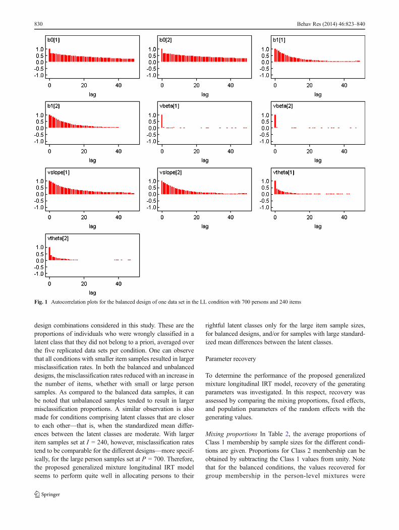
Monitoring convergence Convergence of the MCMC chainswas monitored by examining the time series, kernel density,and autocorrelation plots. In the early steps ofMCMC samplingwithin WinBUGS, the values of the parameters sampled aredependent on the values of the parameters from the previoussteps. This dependence is expected to reduce exponentially asthe sampling continues and to reach a stationary state that

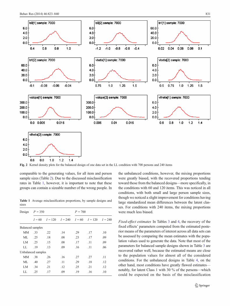
signifies convergence (Bilir, 2009; Lunn et al., 2000). Autocor-relation plots, for instance, provide evidence of how much theconsecutive samples are correlated, and these are expected toapproach the value of zero for all chains as a sign of achievingconvergence. This is portrayed by the sample plots for thedifferent parameters of interest on one simulated data samplein Fig. 1. Convergence can also be monitored from the kerneldensity plots, which are the posterior density plots for theparameters of interest, and a smooth shape for these plots isan indicator of convergence (Bilir, 2009; Lunn et al., 2000). Inthe case of nonconvergence, the kernel density plots of some ofthe parameters are expected to be multimodal and lumpy dis-tributions. As such, the density plots in Fig. 2 provide evidencethat all parameters have converged for this specific data set. Afew exceptions were noted in the intercepts (b01 and b02), mostespecially in those conditions with smaller item and personsamples, as well as in conditions in which the standardizedmean differences between the two latent classes were moderate.

Detection of label switching Two types of label switchingwere investigated in this study. The first one (denotedType I) occurs within a single MCMC chain, when latentclasses change meaning over the estimation chain and canbe detected by the presence of distinct jumps in the time-series plots or multimodal kernel density plots for theMCMC iterations (Stephens, 2000). Figure 2 shows asample of kernel density plots that do not give evidencefor Type I label switching, and this was the case for all ofthe data sets in the considered conditions. The secondtype of label switching (denoted Type II) that we lookedout for occurs when the latent classes switch among thereplicated data sets within the same condition. For exam-ple, in the five replicated data sets of a certain condition,persons initially generated within class g =1 may be con-sistently assigned to class g =2 during the MCMC runsfor the first three of the five data sets, whereas persons inthe other two data sets may be correctly recovered withinclass g =1, which is the class that they were initiallygenerated in. This can be detected by comparing the latentclass-specific parameter estimates with those used in the datageneration, and labels to be applied to each of the latentclasses can be determined (Cho& Cohen, 2010). Type II labelswitching is common in simulation studies and was noticed inthis study. Furthermore, this type of label switching wascommonly observed among smaller person and item samplesizes, and also in the unbalanced conditions. In this study,latent class-specific parameter estimates for all of the data setsin all conditions were compared to those used in data gener-ation, and those parameters whose labels had switched weredetermined and corrected.

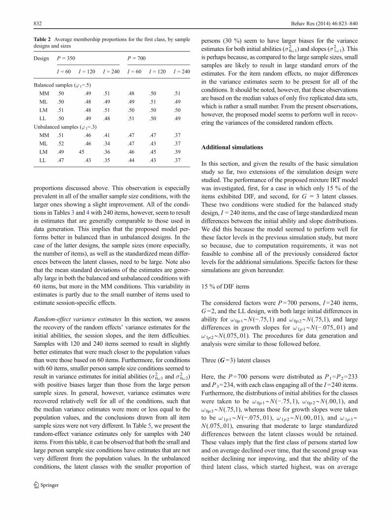
Misclassification proportions Table 1 gives an overview ofthe average misclassification proportions for the different

Behav Res (2014) 46:823–840 829

design combinations considered in this study. These are theproportions of individuals who were wrongly classified in alatent class that they did not belong to a priori, averaged overthe five replicated data sets per condition. One can observethat all conditions with smaller item samples resulted in largermisclassification rates. In both the balanced and unbalanceddesigns, the misclassification rates reduced with an increase inthe number of items, whether with small or large personsamples. As compared to the balanced data samples, it canbe noted that unbalanced samples tended to result in largermisclassification proportions. A similar observation is alsomade for conditions comprising latent classes that are closerto each other—that is, when the standardized mean differ-ences between the latent classes are moderate. With largeritem samples set at I = 240, however, misclassification ratestend to be comparable for the different designs—more specif-ically, for the large person samples set at P = 700. Therefore,the proposed generalized mixture longitudinal IRT modelseems to perform quite well in allocating persons to their

rightful latent classes only for the large item sample sizes,for balanced designs, and/or for samples with large standard-ized mean differences between the latent classes.

Parameter recovery

To determine the performance of the proposed generalizedmixture longitudinal IRT model, recovery of the generatingparameters was investigated. In this respect, recovery wasassessed by comparing the mixing proportions, fixed effects,and population parameters of the random effects with thegenerating values.

Mixing proportions In Table 2, the average proportions ofClass 1 membership by sample sizes for the different condi-tions are given. Proportions for Class 2 membership can beobtained by subtracting the Class 1 values from unity. Notethat for the balanced conditions, the values recovered forgroup membership in the person-level mixtures were

Fig. 1 Autocorrelation plots for the balanced design of one data set in the LL condition with 700 persons and 240 items

830 Behav Res (2014) 46:823–840

comparable to the generating values, for all item and personsample sizes (Table 2). Due to the discussed misclassificationrates in Table 1, however, it is important to note that thesegroups can contain a sizeable number of the wrong people. In

the unbalanced conditions, however, the mixing proportionswere greatly biased, with the recovered proportions tendingtoward those from the balanced designs—more specifically, inthe conditions with 60 and 120 items. This was noticed in allconditions, with both small and large person sample sizes,though we noticed a slight improvement for conditions havinglarge standardized mean differences between the latent clas-ses. For conditions with 240 items, the mixing proportionswere much less biased.

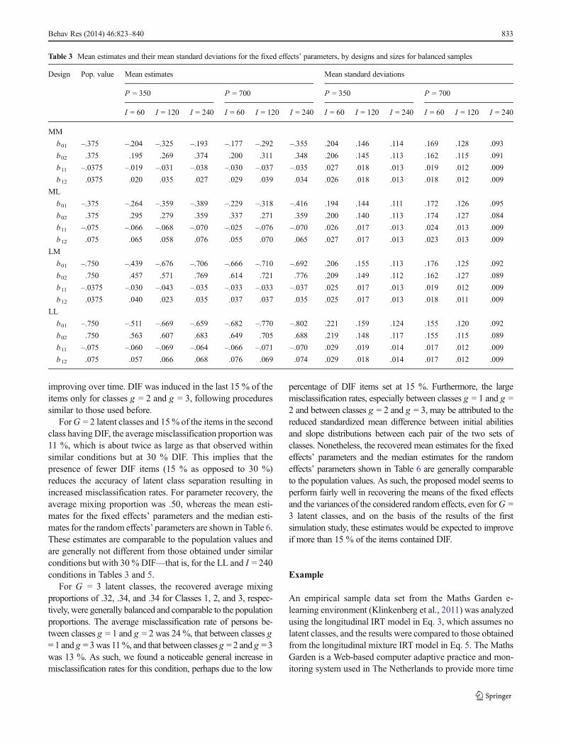
Fixed-effect estimates In Tables 3 and 4, the recovery of thefixed effects’ parameters computed from the estimated poste-rior means of the parameters of interest across all data sets canbe assessed by comparing the mean estimates with the popu-lation values used to generate the data. Note that most of theparameters for balanced sample designs shown in Table 3 arerecovered rather well, because the estimated means are closeto the population values for almost all of the consideredconditions. For the unbalanced designs in Table 4, on theother hand, most conditions have greatly flawed estimates—notably, for latent Class 1 with 30 % of the persons—whichcould be expected on the basis of the misclassification

Fig. 2 Kernel density plots for the balanced design of one data set in the LL condition with 700 persons and 240 items

Table 1 Average misclassification proportions, by sample designs andsizes

Design P = 350 P = 700

I = 60 I = 120 I = 240 I = 60 I = 120 I = 240

Balanced samples

MM .33 .22 .14 .29 .17 .10

ML .25 .18 .08 .23 .17 .09

LM .25 .15 .08 .17 .11 .09

LL .19 .13 .09 .16 .11 .06

Unbalanced samples

MM .38 .26 .16 .27 .27 .11

ML .40 .27 .11 .29 .18 .12

LM .34 .21 .12 .25 .21 .12

LL .25 .17 .09 .19 .16 .10

Behav Res (2014) 46:823–840 831

proportions discussed above. This observation is especiallyprevalent in all of the smaller sample size conditions, with thelarger ones showing a slight improvement. All of the condi-tions in Tables 3 and 4 with 240 items, however, seem to resultin estimates that are generally comparable to those used indata generation. This implies that the proposed model per-forms better in balanced than in unbalanced designs. In thecase of the latter designs, the sample sizes (more especially,the number of items), as well as the standardized mean differ-ences between the latent classes, need to be large. Note alsothat the mean standard deviations of the estimates are gener-ally large in both the balanced and unbalanced conditions with60 items, but more in the MM conditions. This variability inestimates is partly due to the small number of items used toestimate session-specific effects.

Random-effect variance estimates In this section, we assessthe recovery of the random effects’ variance estimates for theinitial abilities, the session slopes, and the item difficulties.Samples with 120 and 240 items seemed to result in slightlybetter estimates that were much closer to the population valuesthan were those based on 60 items. Furthermore, for conditionswith 60 items, smaller person sample size conditions seemed toresult in variance estimates for initial abilities (σ0ω1

2 and σ0ω22 )

with positive biases larger than those from the large personsample sizes. In general, however, variance estimates wererecovered relatively well for all of the conditions, such thatthe median variance estimates were more or less equal to thepopulation values, and the conclusions drawn from all itemsample sizes were not very different. In Table 5, we present therandom-effect variance estimates only for samples with 240items. From this table, it can be observed that both the small andlarge person sample size conditions have estimates that are notvery different from the population values. In the unbalancedconditions, the latent classes with the smaller proportion of

persons (30 %) seem to have larger biases for the varianceestimates for both initial abilities (σ0ω1

2 ) and slopes (σ1ω12 ). This

is perhaps because, as compared to the large sample sizes, smallsamples are likely to result in large standard errors of theestimates. For the item random effects, no major differencesin the variance estimates seem to be present for all of theconditions. It should be noted, however, that these observationsare based on the median values of only five replicated data sets,which is rather a small number. From the present observations,however, the proposed model seems to perform well in recov-ering the variances of the considered random effects.

Additional simulations

In this section, and given the results of the basic simulationstudy so far, two extensions of the simulation design werestudied. The performance of the proposed mixture IRT modelwas investigated, first, for a case in which only 15 % of theitems exhibited DIF, and second, for G = 3 latent classes.These two conditions were studied for the balanced studydesign, I = 240 items, and the case of large standardized meandifferences between the initial ability and slope distributions.We did this because the model seemed to perform well forthese factor levels in the previous simulation study, but moreso because, due to computation requirements, it was notfeasible to combine all of the previously considered factorlevels for the additional simulations. Specific factors for thesesimulations are given hereunder.

15 % of DIF items

The considered factors were P =700 persons, I =240 items,G =2, and the LL design, with both large initial differences inability for ω0p1∼N (−.75,1) and ω0p2∼N (.75,1), and largedifferences in growth slopes for ω 1p1∼N (−.075,.01) andω1p2∼N(.075,.01). The procedures for data generation andanalysis were similar to those followed before.

Three (G =3) latent classes

Here, the P =700 persons were distributed as P1=P2=233and P3=234, with each class engaging all of the I =240 items.Furthermore, the distributions of initial abilities for the classeswere taken to be ω 0p1∼N (−.75,1), ω 0p2∼N (.00,1), andω0p3∼N(.75,1), whereas those for growth slopes were takento be ω 1p1∼N (−.075,.01), ω 1p2∼N (.00,.01), and ω 1p3∼N (.075,.01), ensuring that moderate to large standardizeddifferences between the latent classes would be retained.These values imply that the first class of persons started lowand on average declined over time, that the second group wasneither declining nor improving, and that the ability of thethird latent class, which started highest, was on average

Table 2 Average membership proportions for the first class, by sampledesigns and sizes

Design P = 350 P = 700

I = 60 I = 120 I = 240 I = 60 I = 120 I = 240

Balanced samples (φ1=.5)

MM .50 .49 .51 .48 .50 .51

ML .50 .48 .49 .49 .51 .49

LM .51 .48 .51 .50 .50 .50

LL .50 .49 .48 .51 .50 .49

Unbalanced samples (φ1=.3)

MM .51 .46 .41 .47 .47 .37

ML .52 .46 .34 .47 .43 .37

LM .49 45 .36 .46 .45 .39

LL .47 .43 .35 .44 .43 .37

832 Behav Res (2014) 46:823–840

improving over time. DIF was induced in the last 15 % of theitems only for classes g = 2 and g = 3, following proceduressimilar to those used before.

ForG = 2 latent classes and 15% of the items in the secondclass havingDIF, the average misclassification proportion was11 %, which is about twice as large as that observed withinsimilar conditions but at 30 % DIF. This implies that thepresence of fewer DIF items (15 % as opposed to 30 %)reduces the accuracy of latent class separation resulting inincreased misclassification rates. For parameter recovery, theaverage mixing proportion was .50, whereas the mean esti-mates for the fixed effects’ parameters and the median esti-mates for the random effects’ parameters are shown in Table 6.These estimates are comparable to the population values andare generally not different from those obtained under similarconditions but with 30 % DIF—that is, for the LL and I = 240conditions in Tables 3 and 5.

For G = 3 latent classes, the recovered average mixingproportions of .32, .34, and .34 for Classes 1, 2, and 3, respec-tively, were generally balanced and comparable to the populationproportions. The average misclassification rate of persons be-tween classes g = 1 and g = 2 was 24 %, that between classes g= 1 and g = 3was 11%, and that between classes g = 2 and g = 3was 13 %. As such, we found a noticeable general increase inmisclassification rates for this condition, perhaps due to the low

percentage of DIF items set at 15 %. Furthermore, the largemisclassification rates, especially between classes g = 1 and g =2 and between classes g = 2 and g = 3, may be attributed to thereduced standardized mean difference between initial abilitiesand slope distributions between each pair of the two sets ofclasses. Nonetheless, the recovered mean estimates for the fixedeffects’ parameters and the median estimates for the randomeffects’ parameters shown in Table 6 are generally comparableto the population values. As such, the proposed model seems toperform fairly well in recovering the means of the fixed effectsand the variances of the considered random effects, even forG =3 latent classes, and on the basis of the results of the firstsimulation study, these estimates would be expected to improveif more than 15 % of the items contained DIF.

Example

An empirical sample data set from the Maths Garden e-learning environment (Klinkenberg et al., 2011) was analyzedusing the longitudinal IRT model in Eq. 3, which assumes nolatent classes, and the results were compared to those obtainedfrom the longitudinal mixture IRT model in Eq. 5. The MathsGarden is a Web-based computer adaptive practice and mon-itoring system used in The Netherlands to provide more time

Table 3 Mean estimates and their mean standard deviations for the fixed effects’ parameters, by designs and sizes for balanced samples

Design Pop. value Mean estimates Mean standard deviations

P = 350 P = 700 P = 350 P = 700

I = 60 I = 120 I = 240 I = 60 I = 120 I = 240 I = 60 I = 120 I = 240 I = 60 I = 120 I = 240

MM

b01 –.375 –.204 –.325 –.193 –.177 –.292 –.355 .204 .146 .114 .169 .128 .093

b02 .375 .195 .269 .374 .200 .311 .348 .206 .145 .113 .162 .115 .091

b11 –.0375 –.019 –.031 –.038 –.030 –.037 –.035 .027 .018 .013 .019 .012 .009

b12 .0375 .020 .035 .027 .029 .039 .034 .026 .018 .013 .018 .012 .009

ML

b01 –.375 –.264 –.359 –.389 –.229 –.318 –.416 .194 .144 .111 .172 .126 .095

b02 .375 .295 .279 .359 .337 .271 .359 .200 .140 .113 .174 .127 .084

b11 –.075 –.066 –.068 –.070 –.025 –.076 –.070 .026 .017 .013 .024 .013 .009

b12 .075 .065 .058 .076 .055 .070 .065 .027 .017 .013 .023 .013 .009

LM

b01 –.750 –.439 –.676 –.706 –.666 –.710 –.692 .206 .155 .113 .176 .125 .092

b02 .750 .457 .571 .769 .614 .721 .776 .209 .149 .112 .162 .127 .089

b11 –.0375 –.030 –.043 –.035 –.033 –.033 –.037 .025 .017 .013 .019 .012 .009

b12 .0375 .040 .023 .035 .037 .037 .035 .025 .017 .013 .018 .011 .009

LL

b01 –.750 –.511 –.669 –.659 –.682 –.770 –.802 .221 .159 .124 .155 .120 .092

b02 .750 .563 .607 .683 .649 .705 .688 .219 .148 .117 .155 .115 .089

b11 –.075 –.060 –.069 –.064 –.066 –.071 –.070 .029 .019 .014 .017 .012 .009

b12 .075 .057 .066 .068 .076 .069 .074 .029 .018 .014 .017 .012 .009

Behav Res (2014) 46:823–840 833

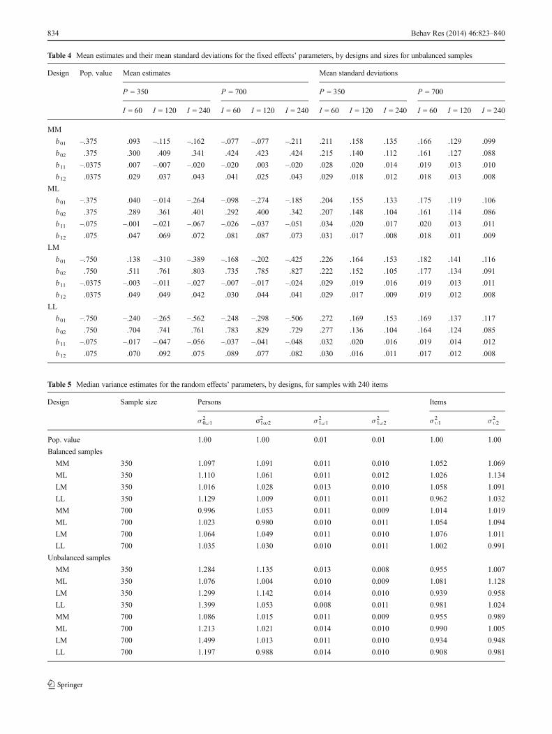
Table 4 Mean estimates and their mean standard deviations for the fixed effects’ parameters, by designs and sizes for unbalanced samples

Design Pop. value Mean estimates Mean standard deviations

P = 350 P = 700 P = 350 P = 700

I = 60 I = 120 I = 240 I = 60 I = 120 I = 240 I = 60 I = 120 I = 240 I = 60 I = 120 I = 240

MM

b01 –.375 .093 –.115 –.162 –.077 –.077 –.211 .211 .158 .135 .166 .129 .099

b02 .375 .300 .409 .341 .424 .423 .424 .215 .140 .112 .161 .127 .088

b11 –.0375 .007 –.007 –.020 –.020 .003 –.020 .028 .020 .014 .019 .013 .010

b12 .0375 .029 .037 .043 .041 .025 .043 .029 .018 .012 .018 .013 .008

ML

b01 –.375 .040 –.014 –.264 –.098 –.274 –.185 .204 .155 .133 .175 .119 .106

b02 .375 .289 .361 .401 .292 .400 .342 .207 .148 .104 .161 .114 .086

b11 –.075 –.001 –.021 –.067 –.026 –.037 –.051 .034 .020 .017 .020 .013 .011

b12 .075 .047 .069 .072 .081 .087 .073 .031 .017 .008 .018 .011 .009

LM

b01 –.750 .138 –.310 –.389 –.168 –.202 –.425 .226 .164 .153 .182 .141 .116

b02 .750 .511 .761 .803 .735 .785 .827 .222 .152 .105 .177 .134 .091

b11 –.0375 –.003 –.011 –.027 –.007 –.017 –.024 .029 .019 .016 .019 .013 .011

b12 .0375 .049 .049 .042 .030 .044 .041 .029 .017 .009 .019 .012 .008

LL

b01 –.750 –.240 –.265 –.562 –.248 –.298 –.506 .272 .169 .153 .169 .137 .117

b02 .750 .704 .741 .761 .783 .829 .729 .277 .136 .104 .164 .124 .085

b11 –.075 –.017 –.047 –.056 –.037 –.041 –.048 .032 .020 .016 .019 .014 .012

b12 .075 .070 .092 .075 .089 .077 .082 .030 .016 .011 .017 .012 .008

Table 5 Median variance estimates for the random effects’ parameters, by designs, for samples with 240 items

Design Sample size Persons Items

σ0ω12 σ1ω2

2 σ1ω12 σ1ω2

2 συ12 συ2

2

Pop. value 1.00 1.00 0.01 0.01 1.00 1.00

Balanced samples

MM 350 1.097 1.091 0.011 0.010 1.052 1.069

ML 350 1.110 1.061 0.011 0.012 1.026 1.134

LM 350 1.016 1.028 0.013 0.010 1.058 1.091

LL 350 1.129 1.009 0.011 0.011 0.962 1.032

MM 700 0.996 1.053 0.011 0.009 1.014 1.019

ML 700 1.023 0.980 0.010 0.011 1.054 1.094

LM 700 1.064 1.049 0.011 0.010 1.076 1.011

LL 700 1.035 1.030 0.010 0.011 1.002 0.991

Unbalanced samples

MM 350 1.284 1.135 0.013 0.008 0.955 1.007

ML 350 1.076 1.004 0.010 0.009 1.081 1.128

LM 350 1.299 1.142 0.014 0.010 0.939 0.958

LL 350 1.399 1.053 0.008 0.011 0.981 1.024

MM 700 1.086 1.015 0.011 0.009 0.955 0.989

ML 700 1.213 1.021 0.014 0.010 0.990 1.005

LM 700 1.499 1.013 0.011 0.010 0.934 0.948

LL 700 1.197 0.988 0.014 0.010 0.908 0.981

834 Behav Res (2014) 46:823–840

to practice and maintain basic arithmetic skills in order toimprove the ability of individual students. Persons can regu-larly engage specific exercise items that are adjusted to theirindividual ability levels using an IRT model, and it includesimmediate feedback to persons on the exercises that theyengage in, thereby ensuring that learning takes place. Accord-ing to Klinkenberg et al., the Maths Garden was speciallydeveloped to improve mathematics education in primaryschools by combining arithmetic practice and measurementin a playful manner using computerized educational games.The data set that was used in Klinkenberg et al.’s article

consisted of data collected in the 2008/2009 academic yearfrom pupils from across The Netherlands, within the age rangeof 4–12 years, enrolled in kindergarten and grades 1–6 ofprimary school. In the present article, however, the analyzeddata set, for the 2010/2011 academic year, consisted of theitem responses of participants 4–18 years of age, with addi-tional, older participants enrolled in the first four years ofsecondary school education. For a detailed design and imple-mentation methodology of the Maths Garden e-learning envi-ronment, we refer the interested reader to Klinkenberg et al.

The four domains of addition, subtraction, multiplication,and division are administered within the Maths Garden envi-ronment, but only the first domain—addition—was analyzedfor this article. The data set consisted of response scores to 610items by 3,803 persons, but the analysis in this article focuseson the 1,335 individuals who engaged in at least 50 exerciseitems and on the 290 items that were answered by at least 150distinct persons. The highest number of engaged items by anindividual was 211, with a median and mean of 69 and 76exercise items, respectively. For each item engaged by anindividual, a time-stamp is recorded automatically by theenvironment. We used this variable—the time at which dis-tinct items were answered by a person—to compute studysessions for the individuals, and one calendar day was used asthe minimum spacing time between two consecutive studysessions for an individual (see, e.g., Cepeda et al., 2008; Vlach& Sandhofer, 2012). For the analyzed data sample, only15.8 % of the considered persons had up to ten study sessions(highest number), whereas 54.5% had up to six study sessions(average number). The response variable was the first attemptscore on an item by a person, with 1 = pass and 0 = fail.

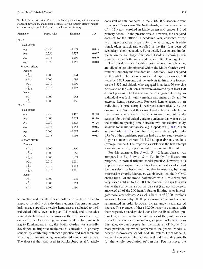
For this example, Eq. 5 with G = 2 latent classes wascompared to Eq. 3 (with G = 1), simply for illustrationpurposes. In normal mixture model practice, however, it isimportant to compare the results of several values of G andthen to select the best-fitting model—for instance, by usinginformation criteria. Moreover, we observed that the MCMCchains for all of the model parameters with G = 2 were notvery stable until up to the 3,000th iteration. Perhaps this wasdue to the sparse nature of this data set (i.e., not all personsanswered all of the 290 items), further limiting us to investi-gate more latent classes. As such, a burn-in of 5,000 iterationswas used, followed by 10,000 post-burn-in iterations that weresummarized in order to obtain the parameter estimates ofinterest. The averages of these 10,000 posterior estimates withtheir respective standard deviations for the fixed effects’ pa-rameters, as well as the median values of the posterior esti-mates for the variance components, are given in Table 7. Fromthis table, we can observe that the mixture IRT Model 5 ismore parsimonious when compared to the general Model 3,because it shows smaller AIC and BIC values. FromModel 3,we get the average initial ability level and the ability growthfor the whole population of persons. For instance, we

Table 6 Mean estimates of the fixed effects’ parameters, with their meanstandard deviations, and median estimates of the random effects’ param-eters for samples with 15 % differential item functioning

Parameter Popn. value Estimate SD

G = 2

Fixed effects

b01 –0.750 –0.679 0.095

b02 0.750 0.727 0.097

b11 –0.075 –0.069 0.009

b12 0.075 0.067 0.010

Random effects

Persons

σ0ω12 1.000 1.094

σ0ω22 1.000 1.099

σ1ω12 0.010 0.010

σ1ω22 0.010 0.012

Items

συ12 1.000 1.085

συ22 1.000 1.056

G = 3

Fixed effects

b01 –0.750 –0.467 0.148

b02 0.000 –0.073 0.136

b03 0.750 0.633 0.126

b11 –0.075 –0.053 0.016

b12 0.000 –0.017 0.013

b13 0.075 0.066 0.013

Random effects

Persons

σ0ω12 1.000 1.360

σ0ω22 1.000 1.166

σ0ω32 1.000 1.109

σ1ω12 0.010 0.011

σ1ω12 0.010 0.013

σ1ω32 0.010 0.011

Items

συ12 1.000 1.075

συ22 1.000 1.063

συ32 1.000 1.080

Behav Res (2014) 46:823–840 835

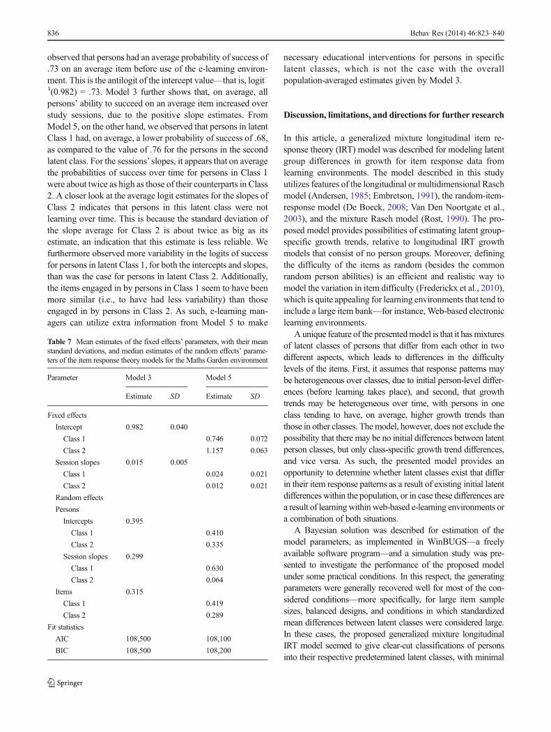
observed that persons had an average probability of success of.73 on an average item before use of the e-learning environ-ment. This is the antilogit of the intercept value—that is, logit–1(0.982) = .73. Model 3 further shows that, on average, allpersons’ ability to succeed on an average item increased overstudy sessions, due to the positive slope estimates. FromModel 5, on the other hand, we observed that persons in latentClass 1 had, on average, a lower probability of success of .68,as compared to the value of .76 for the persons in the secondlatent class. For the sessions’ slopes, it appears that on averagethe probabilities of success over time for persons in Class 1were about twice as high as those of their counterparts in Class2. A closer look at the average logit estimates for the slopes ofClass 2 indicates that persons in this latent class were notlearning over time. This is because the standard deviation ofthe slope average for Class 2 is about twice as big as itsestimate, an indication that this estimate is less reliable. Wefurthermore observed more variability in the logits of successfor persons in latent Class 1, for both the intercepts and slopes,than was the case for persons in latent Class 2. Additionally,the items engaged in by persons in Class 1 seem to have beenmore similar (i.e., to have had less variability) than thoseengaged in by persons in Class 2. As such, e-learning man-agers can utilize extra information from Model 5 to make

necessary educational interventions for persons in specificlatent classes, which is not the case with the overallpopulation-averaged estimates given by Model 3.

Discussion, limitations, and directions for further research

In this article, a generalized mixture longitudinal item re-sponse theory (IRT) model was described for modeling latentgroup differences in growth for item response data fromlearning environments. The model described in this studyutilizes features of the longitudinal or multidimensional Raschmodel (Andersen, 1985; Embretson, 1991), the random-item-response model (De Boeck, 2008; Van Den Noortgate et al.,2003), and the mixture Rasch model (Rost, 1990). The pro-posed model provides possibilities of estimating latent group-specific growth trends, relative to longitudinal IRT growthmodels that consist of no person groups. Moreover, definingthe difficulty of the items as random (besides the commonrandom person abilities) is an efficient and realistic way tomodel the variation in item difficulty (Frederickx et al., 2010),which is quite appealing for learning environments that tend toinclude a large item bank—for instance, Web-based electroniclearning environments.

A unique feature of the presentedmodel is that it hasmixturesof latent classes of persons that differ from each other in twodifferent aspects, which leads to differences in the difficultylevels of the items. First, it assumes that response patterns maybe heterogeneous over classes, due to initial person-level differ-ences (before learning takes place), and second, that growthtrends may be heterogeneous over time, with persons in oneclass tending to have, on average, higher growth trends thanthose in other classes. Themodel, however, does not exclude thepossibility that there may be no initial differences between latentperson classes, but only class-specific growth trend differences,and vice versa. As such, the presented model provides anopportunity to determine whether latent classes exist that differin their item response patterns as a result of existing initial latentdifferences within the population, or in case these differences area result of learningwithin web-based e-learning environments ora combination of both situations.

A Bayesian solution was described for estimation of themodel parameters, as implemented in WinBUGS—a freelyavailable software program—and a simulation study was pre-sented to investigate the performance of the proposed modelunder some practical conditions. In this respect, the generatingparameters were generally recovered well for most of the con-sidered conditions—more specifically, for large item samplesizes, balanced designs, and conditions in which standardizedmean differences between latent classes were considered large.In these cases, the proposed generalized mixture longitudinalIRT model seemed to give clear-cut classifications of personsinto their respective predetermined latent classes, with minimal

Table 7 Mean estimates of the fixed effects’ parameters, with their meanstandard deviations, and median estimates of the random effects’ parame-ters of the item response theory models for the Maths Garden environment

Parameter Model 3 Model 5

Estimate SD Estimate SD

Fixed effects

Intercept 0.982 0.040

Class 1 0.746 0.072

Class 2 1.157 0.063

Session slopes 0.015 0.005

Class 1 0.024 0.021

Class 2 0.012 0.021

Random effects

Persons

Intercepts 0.395

Class 1 0.410

Class 2 0.335

Session slopes 0.299

Class 1 0.630

Class 2 0.064

Items 0.315

Class 1 0.419

Class 2 0.289

Fit statistics

AIC 108,500 108,100

BIC 108,500 108,200

836 Behav Res (2014) 46:823–840

misclassification proportions. Although the results from theutilized simulation study are specific to the considered condi-tions with 350 and 700 persons, comparison of the results fromthe two cases (as well as other preliminary simulations notreported here) provide evidence that the larger the number ofitems, the more likely that the model will provide lower mis-classification rates and more reliable parameter estimates,whether with two or three latent classes. Furthermore, the ob-tained simulation study results appear to support previous sug-gestions regarding potential problems of mixture IRT modelswith small sample sizes of less than 380 persons (cf. Bilir, 2009;Cho, Cohen, & Kim, 2006). In this study, for most conditionswith samples of 350 persons, higher misclassification rates andpoorly recovered model parameters were noted, especially with-in the unbalanced designs. The proposed longitudinal mixtureIRT model was further illustrated with an empirical exampledata set from a Web-based e-learning environment—the MathsGarden (Klinkenberg et al., 2011). The results that we obtainedshowed that the proposed mixture IRT model is a parsimoniousapproach and provides additional latent information when com-pared to the results obtained from a longitudinal IRT model thatassumes no latent classes.

Several limitations of the proposed model have been noted.For instance, the model seems to be unreliable within condi-tions of unbalanced sample sizes or when the standardizedmean differences between latent classes are not large, andmore so for most conditions with item samples of 60 and120. In these cases, the model did not even recover thegenerating parameters very well for the conditions of largeperson sample sizes, with large standardized mean differencesof 1.5 between latent classes for initial abilities as well asslopes (though slightly improved). An additional drawbackthat is commonwithmixture random-item IRTmodels such asthe one considered in the present study is that they cannot berun directly in all common statistical software packages, butrequire flexible software such as WinBUGS. Frederickx et al.(2010) noted that such a limitation can hinder the applicabilityof mixture IRT models, because one needs to be familiar withBayesian statistics, including MCMC computation tech-niques, in order to utilize the model. Moreover, the inferenceprocesses of mixture IRT models using MCMC typicallyrequire substantial computing time in order to obtain usableresults (Cho&Cohen, 2010; von Davier &Yamamoto, 2007).Further research could be aimed at developing or testingalternative methods for fitting the proposed generalized mix-ture longitudinal IRT model in an efficient and quick way—such as by using the gllamm package in the STATA statisticalsoftware (Rabe-Hesketh, Skrondal, & Pickles, 2004b). Fur-thermore, the considered assumption of a linear change of thelatent trait over time may lead to model misspecification and/or to overextraction of classes for the actual data analyses. Theproposed model, however, can easily be extended, and modelfit indices can be used to choose the best-fitting model, after

accounting for the complexity of the models. It is expectedthat more complex models (such as quadratic models) mayrequire even more items and/or persons to yield unbiased andprecise estimates, but an evaluation of these models wasoutside the scope of the present article. Additionally, theprovided simulation study ignored the problem of the accura-cy of estimations of the number of latent classes, because wedid not fit models with different numbers of classes, followedby a model selection procedure to pick the most appropriatenumber. A further evaluation of the proposed modeling ap-proach with respect to the quality of parameter estimates, onthe one hand, and correct model selection, on the other, will beimportant.

Other possible extensions of the proposed modelexist. In this study, for instance, two and three latentperson classes were studied, but more can be introducedin the model by specifying a different value for G inthe WinBUGS macro (see the Appendix). It is alsopossible to study the presence and magnitude of differ-ential functioning items (DIF). This may be achieved,for instance, by extracting class-specific posterior meansof the item difficulty estimates and studying them fur-ther. It would also be interesting to extend the proposedmodel by including manifest person (and perhaps item)properties as predictors, as in the explanatory IRTmodeling framework (De Boeck & Wilson, 2004). Forinstance, the utilized Maths Garden data set comprisedsome manifest person properties, including gender,school, grade, and age, but these were not modeledbecause manifest explanatory modeling was not thefocus of the present article. Bilir (2009), however, notedthat the inclusion of both manifest and latent groups/properties can provide a good comparison on the basisof which to explain or understand the underlying causesof DIF—whether it is due to the presence of manifestgroups, latent classes, or a combination of both. In thespirit of this article, inclusion of such properties mightprovide useful information, in so far as the classificationof growth trends is concerned, whether the differencesin growth trends are due to manifest and/or to latentgroups. Furthermore, the proposed model is limited inthat it is based on the Rasch model, and discriminationparameters were not incorporated. However, actual cor-relations among the items could be made to differ bymaking the Rasch model not fit the actual data well.Future research that takes these issues into account willgreatly improve the proposed model.

Author Note Kind acknowledgments to Han L. J. van der Maas,University of Amsterdam, and to Oefenweb.nl for providing the dataset from the Maths Garden learning environment. We also thank twoanonymous reviewers and Editor in Chief Gregory Francis for theirinsightful comments and suggestions.

Behav Res (2014) 46:823–840 837

Appendix: WinBUGS macro

838 Behav Res (2014) 46:823–840

References

Andersen, E. B. (1985). Estimating latent correlations betweenrepeated testings. Psychometrika, 50, 3–16. doi:10.1007/BF02294143

Andrade, D. F., & Tavares, H. R. (2005). Item response theoryfor longitudinal data: Population parameter estimation.Journal of Multivariate Analysis, 95, 1–22. doi:10.1016/j.jmva.2004.07.005

Bilir, M. K. (2009, July 29).Mixture item response theory-Mimic Model:Simultaneous estimation of differential item functioning for manifestgroups and latent classes. Florida State University. Retrieved fromhttp://diginole.lib.fsu.edu/etd/3761

Bolt, D. M., Cohen, A. S., & Wollack, J. A. (2001). A mixture itemresponse model for multiple-choice data. Journal of Educationaland Behavioral Statistics, 26, 381–409. doi:10.3102/10769986026004381

Cepeda, N. J., Vul, E., Rohrer, D., Wixted, J. T., & Pashler, H. (2008).Spacing effects in learning. A temporal ridgeline of optimal reten-tion. Psychological Science, 19, 1095–1102. doi:10.1111/j.1467-9280.2008.02209.x

Cho, S.-J., Athay, M., & Preacher, K. J. (2013a). Measuring change for amultidimensional test using a generalized explanatory longitudinalitem response model. British Journal of Mathematical andStatistical Psychology, 66, 353–381. doi:10.1111/j.2044-8317.2012.02058.x

Cho, S.-J., Bottge, B., Cohen, A. S., & Kim, S.-H. (2011). Detectingcognitive change in the math skills of low-achieving adolescents.Journal of Special Education, 45, 67–76.

Cho, S.-J., & Cohen, A. S. (2010). A multilevel mixture IRT modelwith an application to DIF. Journal of Educational andBehav io ra l S ta t i s t i c s , 35 , 336–370 . do i : 10 .3102 /1076998609353111

Cho, S.-J., Cohen, A. S., & Bottge, B. (2013b). Detecting interventioneffects using a multilevel latent transition analysis with a mixtureIRT model. Psychometrika, 78, 576–600.

Cho, S.-J., Cohen, A. S., & Kim, S.-H. (2006, June). An investigation ofpriors on the probabilities of mixtures in the mixture Rasch model .Paper presented at the Annual Meeting of the Psychometric Society,Montreal, Canada.

Cho, S.-J., Cohen, A. S., Kim, S.-H., & Bottge, B. (2010). Latenttransition analysis with a mixture IRT measurement model.Applied Psychological Measurement, 34, 583–604.

Cohen, A. S., & Bolt, D. M. (2005). A mixture model analysis ofdifferential item functioning. Journal of EducationalMeasurement, 42, 133–148. doi:10.1111/j.1745-3984.2005.00007

Dai, Y., &Mislevy, R. (2009). A mixture Rasch model with a covariate. Asimulation study via Bayesian Markoc Chian Monte Carlo estima-tion . University of Maryland. Retrieved from http://drum.lib.umd.edu/handle/1903/9926

DeBoeck, P. (2008). Random item IRTmodels. Psychometrika, 73, 533–559. doi:10.1007/s11336-008-9092-x

De Boeck, P., & Wilson, M. (2004). Explanatory item response models: Ageneralized linear and nonlinear approach. NewYork, NY: Springer.

DeMars, C. E., & Lau, A. (2011). Differential item functioning detectionwith latent classes. How accurately can we detect who is respondingdifferentially? Educational and Psychological Measurement, 71,597–616. doi:10.1177/0013164411404221

Desmet, P., Paulussen, H., & Wylin, B. (2006). FRANEL: A publiconline language learning environment, based on broadcast material.In E. Pearson & P. Bohman (Eds.), Proceedings of the WorldConference on Educational Multimedia, Hypermedia andTelecommunications (pp. 2307–2308). Chesapeake VA: AACE.Retrieved from www.editlib.org/p/23329

Embretson, S. E. (1991). A multidimensional latent trait model formeasuring learning and change. Psychometrika, 56, 495–515. doi:10.1007/BF02294487

Finch, W. H., & Pierson, E. E. (2011). A mixture IRT analysis of riskyyouth behavior. Frontiers in Quantitative Psychology andMeasurement, 2, 1–10. doi:10.3389/fpsyg.2011.00098

Fischer, G. H. (1989). An IRT-based model for dichotomouslongitudinal data. Psychometrika, 54, 599–624. doi:10.1007/BF02296399

Fischer, G. H. (1995). Some neglected problems in IRT. Psychometrika,60, 459–487. doi:10.1007/BF02294324

Frederickx, S., Tuerlinckx, F., De Boeck, P., &Magis, D. (2010). RIM: ARandom ItemMixture Model to detect differential item functioning.Journal of Educational Measurement, 47, 432–457. doi:10.1111/j.1745-3984.2010.00122.x

Kamata, A. (2001). Item analysis by the hierarchical generalized linearmodel. Journal of Educational Measurement, 38, 79–93. doi:10.1111/j.1745-3984.2001.tb01117.x

Klinkenberg, S., Straatemeier, M., & Van der Maas, H. L. J. (2011).Computer adaptive practice of maths ability using a new itemresponse model for on the fly ability and difficulty estimation.Computers & Education, 57, 1813–1824. doi:10.1016/j.compedu.2011.02.003

Li, F., Cohen, A. S., Kim, S.-H., & Cho, S.-J. (2009). Model selectionmethods for mixture dichotomous IRT models. AppliedPsychological Measurement, 33, 353–373.

Lunn, D. J., Thomas, A., Best, N., & Spiegelhalter, D. (2000).WinBUGS—A Bayesian modelling framework: Concepts, struc-ture, and extensibility. Statistics and Computing, 10, 325–337.doi:10.1023/A:1008929526011

Miceli, R., Settanni, M., & Vidotto, G. (2008). Measuring change intraining programs: An empirical illustration. Psychology ScienceQuarterly, 50, 433–447.

Mislevy, R., & Verhelst, N. (1990). Modeling item responses whendifferent subjects employ different solution strategies.Psychometrika, 55, 195–215. doi:10.1007/BF02295283

Muthén, B., & Lehman, J. (1985). Multiple group IRT modeling:Applications to item bias analysis. Journal of Educational andBehav io ra l S t a t i s t i c s , 10 , 133–142 . do i : 10 . 3102 /10769986010002133

Paek, I., Baek, S.-G., & Wilson, M. (2012). An IRT modeling ofchange over time for repeated measures item response datausing a random weights linear logistic test model approach.Asia Pacific Education Review, 13, 487–494. doi:10.1007/s12564-012-9210-4

R Development Core Team. (2012). R: A language and environment forstatistical computing. Vienna, Austria: R Foundation for StatisticalComputing. Retrieved from www.R-project.org

Rabe-Hesketh, S., Skrondal, A., & Pickles, A. (2004a).Generalized multilevel structural equation modelling.Psychometrika, 69, 167–190.

Rabe-Hesketh, S., Skrondal, A., & Pickles, A. (2004b). GLLAMMmanual (U.C. Berkeley Division of Biostatistics Working PaperSeries. Working Paper 160). Retrieved from http://biostats.bepress.com/ucbbiostat/paper160

Roberts, J. S., &Ma, Q. (2006). IRT models for the assessment of changeacross repeated measurements. In R. W. Lissitz (Ed.), Longitudinaland value added modeling of student performance (pp. 100–127).Maple Grove, MN: JAM Press.

Rost, J. (1990). Rasch models in latent classes: An integration of twoapproaches to item analysis. Applied Psychological Measurement,14, 271–282. doi:10.1177/014662169001400305

Safer, N., & Fleischman, S. (2005). How student progress monitoringimproves instruction. Educational Leadership, 62, 81–83.

Samuelsen, K. M. (2008). Examining differential item functioning from alatent mixture perspective. In G. R. Hancock & K. M. Samuelsen

Behav Res (2014) 46:823–840 839

(Eds.), Advances in latent variable mixture models (pp. 177–197).Charlotte, NC: Information Age.

Stephens, M. (2000). Dealing with label switching in mixture models.Journal of the Royal Statistical Society, Series B, 62, 795–809. doi:10.1111/1467-9868.00265

VanDenNoortgate,W., &DeBoeck, P. (2005). Assessing and explainingdifferential item functioning using logistic mixed models. Journal ofEducational and Behavioral Statistics, 30, 443–464. doi:10.3102/10769986030004443

Van Den Noortgate, W., De Boeck, P., & Meulders, M. (2003). Cross-classification multilevel logistic models in psychometrics. Journalof Educational and Behavioral Statistics, 28, 369–386. doi:10.3102/10769986028004369

Vlach, H. A., & Sandhofer, C. M. (2012). Distributing learning over time:The spacing effect in children’s acquisition and generalization ofscience concepts. Child Development, 83, 1137–1144.

von Davier, M., Xu, X., & Carstensen, C. H. (2009). Using the generaldiagnostic model to measure learning and change in a longitudinallarge-scale assessment (Technical Report No. ETS RR-09-28).Educational Testing Services. Retrieved from www.ets.org/Media/Research/pdf/RR-09-28.pdf

von Davier, M., & Yamamoto, K. (2007). Mixture-distribution andHYBRID Rasch models. In M. von Davier & C. H. Carstensen(Eds.), Multivariate and mixture distribution Rasch models(Statistics for Social and Behavioral Sciences, pp. 99–115). NewYork, NY: Springer.

840 Behav Res (2014) 46:823–840