A General Option Valuation Approach to Discount for Lack ...

A General Option Valuation Approach to Discount for Lack ofMarketability

Robert Brooks, PhD

A general option-based approach to estimating the discount for lack of marketability

is offered. It is general enough to capture maturity, volatility, hedging availability, and

investor skill, as well as other important factors. The model is shown to contain several

option-based models as special cases. The model also contains two weighting

variables that provide valuation professionals much needed flexibility in addressing the

unique challenges of each nonmarketable valuation assignment. Selected prior

empirical results are reinterpreted with this approach.

Introduction

Many financial instruments are not marketable, such as

private equity, restricted stock in publicly traded

companies, and many over-the-counter financial deriva-

tives contracts. This lack of marketability normally results

in a lower value when compared to an otherwise

equivalent publicly traded instrument. Assigning an

appropriate discount for lack of marketability (DLOM)

is a challenging task requiring both quantitative analysis

and qualitative professional judgment. By definition, any

empirical analysis of DLOM will involve the difficult

problem of positing an appropriate valuation model for

the nonmarketable instrument. The purpose of this paper

is not to resolve this difficult valuation model problem;

the purpose is to offer a new approach for the financial

professional seeking to address this challenging task.

Unlike prior models, the model presented here is

general enough to capture maturity, volatility, hedging

availability, and investor skill, as well as other important

factors, and yet it is easy to interpret and use. Four major

contributions are provided here: First, Longstaff’s (1995)

model is decomposed into two separable components that

can characterize whether the nonmarketable instrument

can be hedged and whether the nonmarketable instrument

owner possesses any sort of skill related to this particular

instrument (for example, market timing ability). Second,

Finnerty’s (2012) model is reinterpreted in a manner that

can be easily justified in practice. Third, Barenbaum,

Schubert, and Garcia’s (2015) model is also reinterpreted

within this new model. Finally, a general option

valuation–based model is introduced that provides an

intellectually rigorous framework yet remains flexible

enough to be applied in practice.

According to Abrams (2010), the first tenuous evidence

of DLOM can be found in the sale of Joseph for twenty

pieces of silver when the going rate was thirty, i.e., a

discount of 33%.1 Stockdale (2013, 13) identifies an

unnamed federal income tax case in 1934 as the first

mention of DLOM. From 1934 through the 1970s, the

admissible DLOM averaged between 20% and 30%.

Based on a 1969 Securities and Exchange Commission

(SEC 1969) document, mutual funds held in excess of

$3.2 billion of restricted equity securities, or about 4.4%

of their total net assets. The SEC recognized that mutual

fund managers would be tempted to report the net asset

value of these restricted securities at or near the current

publicly traded price, creating an instant gain upon which

the manager would be compensated. For example,

suppose a company with $100 publicly traded stock

offered a mutual fund restricted shares at $75. Upon

acquisition, the mutual fund manager would be tempted

to assert the value of the restricted shares at $100,

creating an instant gain of 33%. Thus, the SEC

recognized that ‘‘ ... securities which cannot be readily

sold in the public market place are less valuable than

securities which can be sold ....’’ (SEC 1969, 3) It was not

until 1971 that rigorous academic studies began to appear.

The SEC (1971) conducted a detailed study of trading

data on restricted stock and estimated a DLOM around

26%. Based in part on the 1971 SEC study, the Internal

Robert Brooks is Wallace D. Malone Jr. EndowedChair of Financial Management at The University ofAlabama, phone: (205) 348-8987, e-mail: [email protected]. He is also president of FinancialRisk Management, LLC, phone: (205) 799-9927, e-mail: [email protected].

1See Abrams (2010, 301), along with Genesis 37:28 and Exodus 21:32(Bible). See also Josephus, Antiquities, Book XII, Chapter 11, andLeviticus 27:5.

Business Valuation Reviewe — Winter 2016 35

Business Valuation Reviewe

Volume 35 � Number 4

� 2016, American Society of Appraisers

Revenue Service (1977) issued Revenue Ruling 77-287,

which provides some guidance on estimating an appro-

priate DLOM.

Based on two different restricted stock data sources,

Stockdale documented the existence of discounts from

below –10% (premium) to above 90% (Stockdale 2013,

v. 1, 53). Finnerty reported a range of discounts from –

79% (premium) to 85% based on an analysis of 275

private placements of public equity (Finnerty 2013a, 583,

Table II). Clearly, with such an enormous range of values,

additional tools to address quantifying DLOM would be

helpful.

In the Internal Revenue Service (IRS) publication,

‘‘Discount for Lack of Marketability Job Aid for IRS

Valuation Professionals’’ dated September 25, 2009, page

4, the authors make the following standard definitions as

well as provide a few important observations: (italics and

footnotes in the original)

Marketability is defined in the International Glossary ofBusiness Valuation Terms as ‘‘the ability to quickly convert

property to cash at minimal cost.’’2 Some texts go on to add

‘‘with a high degree of certainty of realizing the anticipated

amount of proceeds.’’3

A Discount for Lack of Marketability (DLOM) is ‘‘an

amount or percentage deducted from the value of an

ownership interest to reflect the relative absence of

marketability.’’4

...

In the alternative [non-marketable instrument], a lesser price

is expected for the business interest that cannot be quickly

sold and converted to cash. A primary concern driving this

price reduction is that, over the uncertain time frame

required to complete the sale, the final sale price becomes

less certain and with it a decline in value is quite possible.

Accordingly, a prudent buyer would want a discount for

acquiring such an interest to protect against loss in a future

sale scenario.

While there are numerous technical issues and subtle

nuances, the goal of the DLOM exercise is to monetize

the uncertainty surrounding the lack of marketability.

Generally, it is a normative question: What ought to be

the DLOM for this specific case? Obviously, there is

never direct evidence for a specific case. Valuation

professionals use data from numerous sources that

provide indirect evidence, such as restricted stock studies.

Not surprisingly, given the enormous amount of money

involved in DLOM estimation, this indirect evidence

often leads to vastly different valuations depending on

your objective (for example, IRS or taxpayer). Also, there

are many other potential discounts that are not addressed

here, including minority interest discount, other transfer-

ability restriction discounts, and nonsystematic risk

discounts.5

Approaches to estimating DLOM can be generally

categorized as either empirical or theoretical. Empirical

approaches typically focus on market evidence from

restricted stock transactions, various private placements,

and private investments in public equities. One then must

extrapolate from the market evidence to the particular

case at hand. Given the unique attributes of every case,

this extrapolation can be quite tenuous. For a concise

summary of an extensive set of empirical studies, see

Stockdale (2013, 47–49).

Theoretical approaches are attractive because they

typically provide a parsimonious set of inputs that can

be estimated for each DLOM assignment. Theoretical

models are generally either based on discounted cash flow

models or option valuation models. For examples of the

discounted cash flow models, see Meulbroek (2005),

Tabak (2002), and Stockdale (2013); see also Mercer’s

quantitative marketability discount model (Stockdale

2013, 232–238).

In this paper, the model is built on existing DLOM

literature related to option theory to provide a general

framework for estimating DLOM that can be used in a

wide array of applications. Presently, option-based

DLOM approaches are rudimentary and often provide

only an upper bound. An implicit problem is the

underlying instrument is assumed to lack liquidity, and

modern option theory relies heavily on liquid underlying

instruments. This problem is not unique, as evidenced by

real options applications. The framework developed here

is easily modified to incorporate both risk-adjusted

growth rates of the underlying instrument, as well as

risk-adjusted discount rates. The focus here is not to

overcome the numerous challenges of applying option

theory in illiquid markets; rather, the focus is to

generalize and extend existing DLOM estimation tech-

niques already widely used in practice.

This unique approach decomposes existing models into

a skill component and a hedge component. The skill

component measures the DLOM attributable to the

economic value lost for talented investors who suffer

solely because the underlying instrument is not market-

able. That is, if the underlying instrument were

2International Glossary of Business Valuation Terms, as adopted in 2001by the American Institute of Certified Public Accountants, AmericanSociety of Appraisers, Canadian Institute of Chartered BusinessValuators, National Association of Certified Valuation Analysts, andThe Institute of Business Appraisers.3Shannon P. Pratt, and Alina V. Niculita, Valuing a Business, TheAnalysis and Appraisal of Closely Held Businesses, 5th ed. (New York:McGraw Hill, 2008), 39.4International Glossary of Business Valuation Terms.

5I also do not address the closely related discount for lack of liquidity(see IRS 2009, 5).

Page 136 � 2016, American Society of Appraisers


marketable, then this investor would be better off at the

end of the nonmarketable period. The hedge component

measures the DLOM attributable to the inability to hedge

adverse market price movements solely because the

underlying instrument is not marketable.

For example, the DLOM for restricted stock of a highly

skilled chief executive officer (CEO) would be signifi-

cantly different from the DLOM of the same restricted

stock when estimating the estate taxes if this same CEO

passed away.6 The decomposition herein provides

valuation professionals needed flexibility to address a

wide array of DLOM valuation problems. This paper

demonstrates that the model has existing option-based

models as special cases.

The primary advantage of this model is the ability to

explicitly address several important features common to

DLOM problems. These features include the ability to

externally hedge and the timing ability of the instrument

owner. This model provides professionals much needed

discretion and is not based on directly observable

phenomenon. Unfortunately, not one single DLOM

estimation approach can be based on directly observable

phenomenon by its very nature. Each DLOM estimation

assignment has a unique underlying instrument as well as

a unique property owner. Thus, DLOM requires profes-

sional judgment, and the DLOM tools should provide this

needed flexibility to reflect these judgments.

The focus here is option valuation–based monetization

of the lack of marketability. The remainder of the paper is

organized as follows. First, I discuss the relevant option

valuation–based DLOM literature. In the next section, the

option-based DLOM model is introduced, and its

decomposition is explained. Then, I illustrate the model

and provides alternative interpretations of some existing

empirical evidence. The last section presents the

conclusions.

Option Valuation–Based DLOM Literature

There is a vast literature that addresses estimating

DLOM. For a review of this literature, as well as current

DLOM estimation practices, see Stockdale (2013). This

paper focuses solely on option valuation–based DLOM

approaches.

European style put option

Chaffe (1993, 182) summarizes, ‘‘if one holds

restricted or non-marketable stock and purchases an

option to sell those shares at the free market price, the

holder has, in effect, purchased marketability for the

shares. The price of the put is the discount for lack of

marketability.’’ The acquisition of a put option eliminates

the uncertainty of the future downside risk. The shares

have essentially been insured against any event that

drives the price down. Recall, however, that the put

option does not eliminate the benefits that accrue when

the share price rises. Thus, this put option is an upper

bound for DLOM, at best. Chaffe proposes using the cost

of capital for the interest rate in the Black-Scholes-Merton

option valuation model (BSMOVM). Chaffe further

illustrates the DLOM using volatilities from 60% to 90%.

The BSMOVM is based on the assumption that the

underlying instrument follows geometric Brownian

motion, implying the terminal distribution is lognormal.7

The lognormal distribution has several well-known

weaknesses, including the inability of the underlying

instrument to be zero and taking on unusual features with

high volatility.8 Unfortunately, DLOM is often estimated

for highly volatile instruments and relatively long

horizons. The terminal volatility is linear in the square

root of maturity time (rffiffiffiffiffiffiffiffiffiffiffiT � tp

). Assuming a one-year

horizon, when terminal volatility exceeds 100%, the

lognormal distribution appears dubious at best. Often,

estimated volatility exceeds 100%. For example, if the

stock price is $100 with $100 strike price and terminal

volatility of 100% (with interest rates and dividend yield

assumed to be zero), then based on the lognormal

distribution assumption, although the mean is $100, the

median is $61, and the mode is $22 (skewness is 6.2, and

excess kurtosis is 111). Given that stock returns tend to be

negatively skewed, these statistics are inconsistent with

observed stock price behavior. Although 100% terminal

volatility seems high, it is equivalent to a four-year (6.25-

year) horizon and 50% (40%) annual volatility. There-

fore, DLOM estimates based on option-valuation ap-

proaches require significant professional judgment.

Several authors have extended Chaffe’s work by

examining longer maturity options. See, for example,

Trout (2003) and Seaman (2005a, 2005b, 2007, 2009).

Barenbaum, Schubert, and Garcia (2015) combined the

long put position with a short call position and analyzed

DLOM based on this collar position. They examined the

inherent basis risk when the options are based on a

financial instrument other than the one being discounted.

6I assume the terms of the restriction were not contingent on the CEObeing alive.

7Remember that distributions are not observable. Finance is neitherphysics nor mathematics—it is a human science. Future stock pricechanges reflect a myriad of human decisions, and any distribution ismerely a conjecture of the potentials going forward.8For more details, see Brooks and Chance (2014). One example of anunusual feature is if the stock price is $100, the expected return is 12%(annualized, continuously compounded), the standard deviation is 75%(annualized, continuously compounded), and the horizon is two years,then the mode is about $13.

Business Valuation Reviewe — Winter 2016 Page 137

A General Option Valuation Approach to Discount for Lack of Marketability

Interestingly, Chaffe (1993, 182) notes ‘‘There is also a

component of the discount that is related to the inability

to realize an intermediate gain quickly and efficiently. For

purposes of this analysis, we forego quantification of the

discount factor associated with this second aspect of

marketability.’’ Longstaff incorporates this aspect with a

lookback put option.

Lookback put option

Longstaff (1995) captures the intermediate gain issue

by assuming the investor has skill or perfect timing

ability. He develops an upper bound estimate for DLOM

based on a floating strike lookback put option model.

Longstaff (1995, 1774) concludes, ‘‘The results of this

analysis can be used to provide rough order-of-magnitude

estimates of the valuation effects of different types of

marketability restrictions. In fact, the empirical evidence

suggests that the upper bound may actually be a close

approximation to observed discounts for lack of market-

ability. More importantly, however, these results illustrate

that option-pricing techniques can be useful in under-

standing liquidity in financial markets and that liquidity

derivatives have potential as tools for managing and

controlling the risk of illiquidity.’’I present a more general version of Longstaff’s model.

Note that Longstaff assumes the lookback maximum is

expressed as MT¼max0�s�T[Vser(T�s)], where Vs denotes

the underlying instrument’s value at time s, the risk-free

interest rate is r, and the time to maturity is T. Assuming

the underlying instrument grows at the risk-free rate from

the time of maximum value until the option maturity has

the effect of removing the interest rate from the final

model. I assume the more traditional case of M̂T ¼max0�s�T[Vs] and then consider the special case of

Longstaff. Longstaff’s model is equivalent to the more

traditional lookback option structure if one assumes that

the risk-free interest rate is zero.

Average-strike put option

Finnerty (2012, 2013a) introduces an average-strike put

option approach to approximating DLOM. Finnerty

assumes standard dividend adjusted geometric Brownian

motion, as well as assuming the instrument holder has no

special skill (e.g., market-timing ability). Finnerty’s

model is based on assuming an average forward price

that relies on the standard carry arbitrage formula.

Finnerty’s model effectively provides DLOM estimates

roughly 50% lower than an equivalent plain-vanilla put

option (see detailed discussion in the next section).

Finnerty (2012, 67) concludes, ‘‘The average-strike put

option model ... calculates marketability discounts that

are generally consistent with the discounts observed in

letter stock private placements, although there is a

tendency to understate the discount when the stock’s

volatility is under 45 percent or over 75 percent,

especially for longer restriction periods. The marketabil-

ity discounts implied by observed private placement

discounts reflect[s] differences in stock price volatility, as

option theory and the average-strike put option model

predict.’’ For an interpretation of these first three models,

see Abbott (2009) and Finnerty (2013b).

Equity collar

Barenbaum, Schubert, and Garcia (2015) document

that, absent timing ability, a put option overstates DLOM.

Further, if a put option can be reasonably approximated,

then surely a call option can be estimated also. Thus,

through a combination of a call option, a put option, and a

loan, the DLOM can be approximated without the known

overstatement. The key variable determining the DLOM

is the interest rate spread between the appropriate lending

rate and the risk-free rate. For a critique of the

Barenbaum, Schubert, and Garcia (BSG) model, see

Finnerty and Park (2015).

I now turn to introduce the general option-based

DLOM and the flexibility to decompose it into compo-

nent pieces.

Option-Based DLOM and Decomposition

Longstaff’s model provides both the direct measure of

a plain-vanilla put option introduced by Chaffe, as well as

the lookback feature measuring the economic value lost

from perfect timing. Unfortunately, Longstaff’s model is

merely an upper bound.

Four major issues are addressed here. First, based on

Longstaff’s model, I decompose the standard floating

strike lookback put option into two components, a plain-

vanilla put option and a term I define as the residual

lookback portion. Second, I apply this decomposition to

Longstaff’s model and explore its implications by

reexamining some of his results. Third, I provide a

simple alternative interpretation to Finnerty’s model and

introduce a weighting system. Empirically, Finnerty’s

model fits some data well, but the economic intuition is

difficult. Fourth, I reconfigure the BSG model, demon-

strating that it provides an important alternative interpre-

tation for the general model explored here. Finally, I

present the general option-based DLOM model and

explore some simple, but extreme, cases.

I have explored DLOM models where the underlying

instrument lacks marketability yet option-based solutions

appear reasonable. Here, I streamline the existing DLOM

option-based models and provide a general framework for

a wide array of applications. The key feature here is



flexibility. Unfortunately, the cost is a less parsimonious

model. Professionals seeking to apply this framework can

easily reduce the number of estimated parameters.

Decomposition of floating strike lookback putoption model

Let LP̂tðVt; M̂tÞ denote the value at time t of a floating

strike lookback put option on the underlying instrument,

Vt, where M̂t ¼ max0�s�T[Vs]. One way to express the

option value is based on two separate components

LP̂tðVt; M̂tÞ ¼ P̂tðVt; M̂tÞ þ L̂tðVt; M̂tÞ; ð1Þ

where P̂tðVt; M̂tÞ denotes the plain vanilla put portion,

and L̂tðVt; M̂tÞ denotes the residual lookback portion. I

now examine each portion separately. The general option-

based DLOM introduced later will be based on this

decomposition.

Component 1: Plain vanilla put portion (Blackand Scholes 1973; Merton 1973)

Based on the BSMOVM, we have

PtðVt;XÞ ¼ Xe�rðT�tÞNð�d2Þ � Vte�dðT�tÞNð�d1Þ; ð2Þ

where

d1 ¼ln Vt

X

� �þ r � dþ r2

2

� �ðT � tÞ

rffiffiffiffiffiffiffiffiffiffiffiT � tp ; ð3Þ

d2 ¼ d1 � rffiffiffiffiffiffiffiffiffiffiffiT � tp

; ð4Þ

and

NðdÞ ¼Z d

�‘

nðxÞdx ¼Z d

�‘

e�x2

2ffiffiffiffiffiffi2pp dx

(standard normal cumulative distribution function).

Here,

T time to expiration, measured in years, where the

option is assumed to be evaluated at time t,

r known, annualized, continuously compounded ‘‘risk-

free’’ interest rate,

d known, annualized, continuously compounded divi-

dend yield,

r known, annualized standard deviation of continu-

ously compounded percentage change in the under-

lying instrument’s price,

Vt observed value of the underlying instrument at time t,

X strike or exercise price, and

Pt model value of a plain-vanilla put option.

As I will discuss later, the DLOM is influenced by

dividend policy, and this model captures this influence.

Note that if the put option is at the money (Vt¼X) and if r¼ d¼ 0, then this expression can be significantly reduced

to

P̂t ¼ Pt ¼ Vt 2NrffiffiffiTp

2

� �� 1

: ð5Þ

This expression is important to understanding both the

Longstaff and Finnerty models.

Component 2: Residual lookback portion

Based on the BSMOVM framework, the residual

lookback portion can be expressed as9

L̂tðVt; M̂tÞ ¼ Vte�rðT�tÞ r2

2ðr � dÞ

3 eðr�dÞðT�tÞNðd1Þ �Vt

M̂t

� ��2ðr�dÞ=r2

Nðd3Þ" #

r 6¼ dÞ;ð ð6aÞ

L̂tðVt; M̂tÞ ¼ Vte�rðT�tÞ

3

�r2ðT � tÞ

2Nðd1Þ þ r

ffiffiffiffiffiffiffiffiffiffiffiT � tp

nðd1Þ

þ lnVt

M̂t

Nðd3Þ

�ðr ¼ dÞ; ð6bÞ

where

d3 ¼ d1 �2ðr � dÞ


r; and ð7Þ

nðdÞ ¼ e�d2

2ffiffiffiffiffiffi2pp

(standard normal probability density function).

Again, if the residual lookback portion is at the money

(Vt ¼ X) and r ¼ d ¼ 0, then this expression can be

reduced significantly to

L̂t ¼ Lt

¼ Vtr2ðT � tÞ

2N

rffiffiffiffiffiffiffiffiffiffiffiT � tp

2

� �þ r


nrffiffiffiffiffiffiffiffiffiffiffiT � tp

2

� �� :

ð8Þ

I will discuss these results in detail when I present the

general option-based DLOM model. First, I highlight

several new insights from Longstaff’s model in the

context of this decomposition. After exploring insights

related to Finnerty’s model and BSG’s model, I will

introduce the general option-based DLOM model.

9This well-known result can be found in Haug (2007, 142), Wilmott(2000, v. 1, 282), as well as other places. A detailed derivation of thefloating strike lookback put is also available from the author.



Decomposition of Longstaff’s model

The general option-based DLOM model is based on

decomposing Longstaff’s model and then applying

appropriate weights to each component. Therefore, I turn

now to decomposing the Longstaff model and provide

important new insights along the way.

Note when Vt ¼ M̂t (at-the-money) and r ¼ d ¼ 0 (no

dividends and no underlying instrument carry cost), then

M̂T ¼ MT ¼ maxt�s�T ½Vs�, and the results are equivalent

to Longstaff’s model. That is,

LPtðVt ¼ Mt;MtÞ ¼ Pt þ Lt; ð9Þ

where

Pt ¼ Vt 2NrffiffiffiffiffiffiffiffiffiffiffiT � tp

2

� �� 1

� �ð10Þ

(Longstaff’s plain-vanilla put portion), and

Lt ¼ Vtr2ðT � tÞ

2N


2

� �þ r


nrffiffiffiffiffiffiffiffiffiffiffiT � tp

2

� �� ð11Þ

(Longstaff’s residual lookback portion).

Generally, for low volatility and short horizons,

roughly half of the lookback put option value is

composed of the plain-vanilla put portion, and the other

half is the residual lookback portion.

With longer time to maturity and higher volatilities, the

residual lookback portion is significantly greater than the

plain-vanilla put portion. The decomposition provided

here is important because it sheds light on two important

aspects of DLOM, the downside insurance provided by

the plain-vanilla put option and the economic loss from

the inability to incorporate investor skill. Both of these

aspects can vary depending on the DLOM application.

This decomposition is exploited to construct a more

flexible DLOM tool. Recall, the empirical evidence seems

to support Finnerty’s model as providing reasonable

estimates of the economic value for the DLOM.

Alternative interpretation of Finnerty’s model

Finnerty (2012) introduced a DLOM model based on

an average-strike put option. Further, he asserted ‘‘the

model-predicted marketability discounts are consistent

with actual private placement discounts after adjusting for

the information, ownership concentration, and overvalu-

ation effects that accompany a stock private placement’’

(Finnerty 2012, 53). As Finnerty’s model does not appear

to fit well with other existing models, and an average-

strike approach is difficult to justify, I show an alternative

interpretation as well as important features of his model.

Based on the notation already presented and some

rearranging, Finnerty’s DLOM model when expressed in

dollars is

DLOM$;Finnerty ¼ Vte�dðT�tÞ 2N

mffiffiffiffiffiffiffiffiffiffiffiT � tp

2

� �� 1

� �; ð12Þ

where10

m2ðT � tÞ ¼ r2ðT � tÞþ ln 2

�er2ðT�tÞ � r2ðT � tÞ � 1

�n o� 2 ln er2ðT�tÞ � 1

n o, ln 2f g: ð13Þ

Due to the upper limit on the volatility time term

(m2ðT � tÞ, lnf2g), the upper limit on Finnerty’s DLOM

model is (assuming d ¼ 0)

DLOM%;Finnerty ¼ 2N

ffiffiffiffiffiffiffiffiffiffiffiln 2f g

p2

!� 1 ¼ 32:28%:

Often DLOM is observed to exceed this upper limit, so

Finnerty’s model is severely limited.

Recall Finnerty assumes the residual lookback portion

is zero. Consider a plain-vanilla put option with a strike

price equal to the at-the-forward price X ¼ Ft ¼Vte

(r�d)(T�t); thus, the option can be expressed simply as11

Pt

�Vt;X ¼ Vte

ðr�dÞðT�tÞ�

¼ Vte�dðT�tÞ 2N


2

� �� 1

� �:

This simple plain-vanilla at-the-forward put option result

is equivalent to Finnerty’s model except for the volatility

term. Note that r.m.0 when volatility is positive and

time to maturity is positive. Let pm [ mr denote the

proportion of Finnerty’s parameter when compared with

the underlying instrument’s volatility. Although not

shown here, except for very low volatility, short

maturities and high-volatility, long maturities, the pro-

portion term (pm) is relatively stable around 57%. Based

on Finnerty’s assertion regarding letter stock, then the

residual lookback put portion should be zero, and only a

portion of the plain-vanilla put option is reflected in the

DLOM. This interpretation makes sense because a put

option provides more than just marketability; it provides

protection from unanticipated declines in value.

10Note that ln{2(er2ðT�tÞ �r2(T� t)�1)}¼ ln{2}þ ln{er2ðT�tÞ �r2(T� t)� 1}, and the limit as r2(T� t) � ‘ is ln{er2ðT�tÞ � 1} � r2(T� t) andln{er2ðT�tÞ � r2(T � t) � 1} � r2(T � t).11We assume a fully arbitraged market; hence, the equilibrium forwardprice is as expressed above. Clearly, in markets where arbitrage activityis limited, then this forward expression is not appropriate. Most smallcapitalization stocks do not have an active forward market, limiting thismodel’s realism.



Therefore, with the proportion defined above,

mathematically Finnerty’s model can simply be ex-

pressed as

DLOM$;Finnerty ¼ Vte�dðT�tÞ 2N

pmrffiffiffiffiffiffiffiffiffiffiffiT � tp

2

� �� 1

� �:

ð14Þ

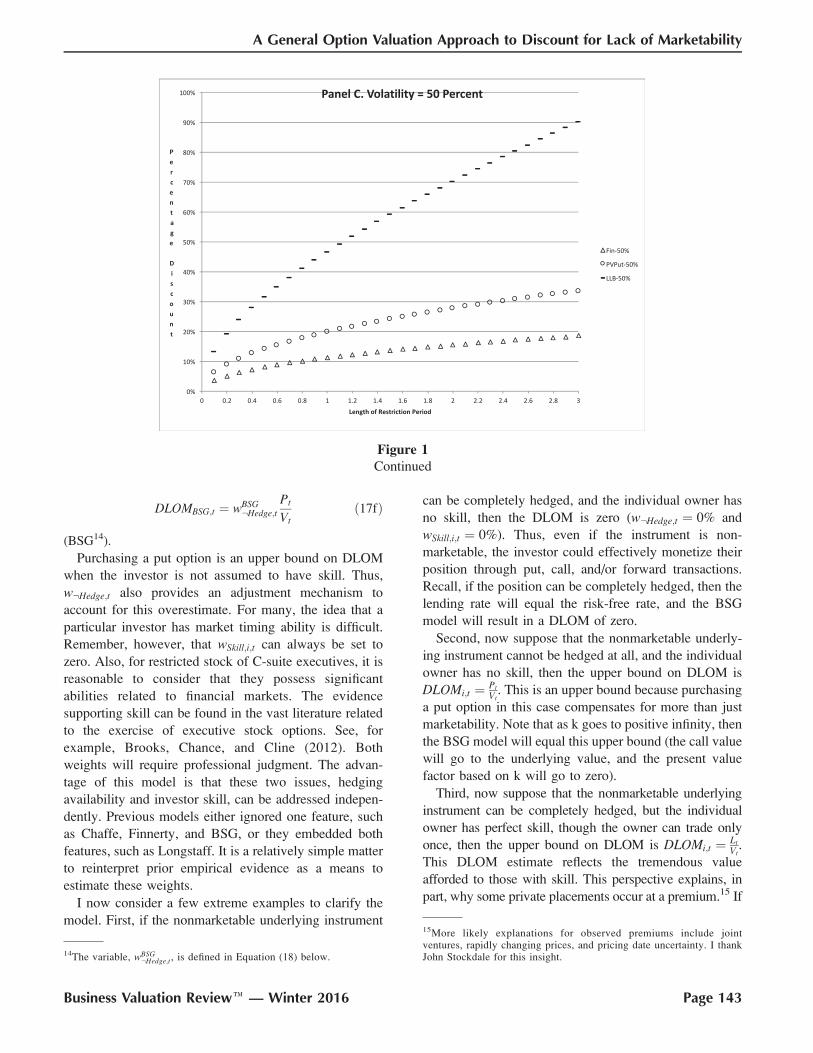
Figure 1 replicates Finnerty’s Exhibit 2 with the

inclusion of the plain-vanilla put option model. The

results are presented in three panels for clarity. Clearly,

Longstaff’s lookback put option model results in much

higher discounts when compared to the other two models.

Finnerty’s model is always less than the plain-vanilla put

option model as his model is equivalent to using a

proportionally lower volatility (pm).

Alternative interpretation of BSG’s model

Barenbaum, Schubert, and Garcia proposed a DLOM

estimate based on a combination of a call option, a put

option, and a loan. Specifically,

DLOM%;BSG ¼Vt � Vte

�kðT�tÞ þ CtðVt;XÞ � PtðVt;XÞVt

;

ð15Þ

where k denotes the lending rate, C denotes the call

option, and the strike price, X, is equal to the underlying

value (Vt). Based on put-call parity,

DLOM%;BSG ¼ e�rðT�tÞ � e�kðT�tÞ: ð16Þ

Clearly, the interest rate spread (k� r) is the key driver for

the DLOM within the BSG model.

Building on this previous theoretical work and

empirical insights, I now propose a general option-based

DLOM model.

General option-based DLOM

I introduce a weighting scheme that is general

enough to handle most DLOM problems. First, the

degree of external hedging opportunities will directly

influence DLOM. If hedging opportunities could be

pursued, then the DLOM applies only to the proportion

of the underlying instrument’s volatility that cannot be

hedged. Recall if 100% of the volatility can be hedged

without costs, then the DLOM related solely to

downside risk should be zero.12 That is, if a put option

is available to purchase that eliminates the nonmarket-

able instrument’s downside risk, then a call option is

likely also available to sell that will offset the cost of

the put option and guarantee the future sale price, and

the lending rate will equal the risk-free rate.13 I assume

the external hedging opportunities are not specific to

the investor. Clearly, if a particular investor is excluded

from available hedging opportunities due to regulation

or corporate culture, then this portion of the DLOM

applies.

Second, the degree of investor skill will also directly

influence DLOM. If a particular investor evidences some

capacity for say market timing, then the lack of

marketability imposes a significant expense. Clearly,

perfect skill with active trading would result in near-

infinite profits in a short period of time within the

standard option valuation paradigm. Therefore, I propose

the following general options-based DLOM (express as a

percentage of the underlying instrument’s fully market-

able value):

DLOMi;t ¼ w:Hedge;tPt

Vtþ wSkill;i;t

Lt

Vt; ð17Þ

where Pt and Lt are as defined in Equations (2) and (6),

respectively. Let w:Hedge;t denote the investor-indepen-dent proportion of the underlying instrument that cannot

be hedged, and let wSkill;i;t denote the investor-dependentproportion of the underlying instrument that reflects the

investor’s skill (e.g., market timing).

The following are special cases of this model:

DLOMPut;t ¼Pt

Vtð17aÞ

(European-style put),

DLOMChaffe;t ¼Ptðr ¼ Cost Of CapitalÞ

Vtð17bÞ

(Chaffe),

DLOMGeneral Lookback;t ¼P̂t

Vtþ L̂t

Vt; ð17cÞ

(general lookback),

DLOMLongstaff ;t ¼Ptðr ¼ 0; d ¼ 0Þ

Vtþ Ltðr ¼ 0; d ¼ 0Þ

Vt

ð17dÞ

(Longstaff),

DLOMFinnerty;t ¼Ptðr ¼ mÞ

Vtð17eÞ

(Finnerty), and

12Ignoring the skill argument made below. Also, hedging alwaysinvolves costs; hence, the DLOM will simply be the cost of hedging.

13As previously mentioned, this is a simple illustration of the well-known put-call parity relationship. Clearly, tax consideration may resultin using a zero-cost collar or other tax-efficient strategy.



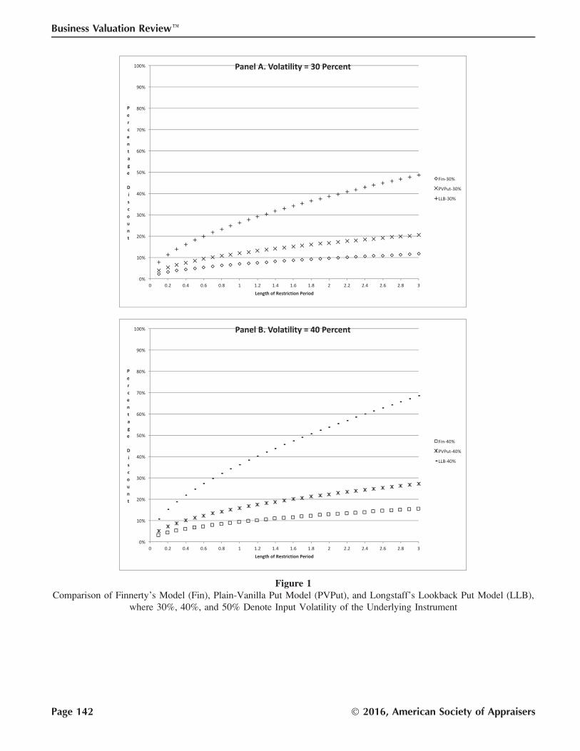
Figure 1Comparison of Finnerty’s Model (Fin), Plain-Vanilla Put Model (PVPut), and Longstaff’s Lookback Put Model (LLB),

where 30%, 40%, and 50% Denote Input Volatility of the Underlying Instrument



DLOMBSG;t ¼ wBSG:Hedge;t

Pt

Vtð17fÞ

(BSG14).

Purchasing a put option is an upper bound on DLOM

when the investor is not assumed to have skill. Thus,

w:Hedge;t also provides an adjustment mechanism to

account for this overestimate. For many, the idea that a

particular investor has market timing ability is difficult.

Remember, however, that wSkill;i;t can always be set to

zero. Also, for restricted stock of C-suite executives, it is

reasonable to consider that they possess significant

abilities related to financial markets. The evidence

supporting skill can be found in the vast literature related

to the exercise of executive stock options. See, for

example, Brooks, Chance, and Cline (2012). Both

weights will require professional judgment. The advan-

tage of this model is that these two issues, hedging

availability and investor skill, can be addressed indepen-

dently. Previous models either ignored one feature, such

as Chaffe, Finnerty, and BSG, or they embedded both

features, such as Longstaff. It is a relatively simple matter

to reinterpret prior empirical evidence as a means to

estimate these weights.

I now consider a few extreme examples to clarify the

model. First, if the nonmarketable underlying instrument

can be completely hedged, and the individual owner has

no skill, then the DLOM is zero (w:Hedge;t ¼ 0% and

wSkill;i;t ¼ 0%). Thus, even if the instrument is non-

marketable, the investor could effectively monetize their

position through put, call, and/or forward transactions.

Recall, if the position can be completely hedged, then the

lending rate will equal the risk-free rate, and the BSG

model will result in a DLOM of zero.

Second, now suppose that the nonmarketable underly-

ing instrument cannot be hedged at all, and the individual

owner has no skill, then the upper bound on DLOM is

DLOMi;t ¼ Pt

Vt. This is an upper bound because purchasing

a put option in this case compensates for more than just

marketability. Note that as k goes to positive infinity, then

the BSG model will equal this upper bound (the call value

will go to the underlying value, and the present value

factor based on k will go to zero).

Third, now suppose that the nonmarketable underlying

instrument can be completely hedged, but the individual

owner has perfect skill, though the owner can trade only

once, then the upper bound on DLOM is DLOMi;t ¼ Lt

Vt.

This DLOM estimate reflects the tremendous value

afforded to those with skill. This perspective explains, in

part, why some private placements occur at a premium.15 If

Figure 1Continued

14The variable, wBSG:Hedge;t, is defined in Equation (18) below.

15More likely explanations for observed premiums include jointventures, rapidly changing prices, and pricing date uncertainty. I thankJohn Stockdale for this insight.



the investor skill is unique to a particular set of underlying

instruments, then the investor may be willing to pay a

premium for the instrument for the opportunity to exercise

their skill. The value to the investor of the position is

Vt þ Lt, and there may be times when the particular

investor cannot acquire the instrument in the traded market.

I focus here solely on DLOM cases.

Fourth, now suppose that the nonmarketable underly-

ing instrument cannot be hedged, and the individual

owner has perfect skill, but can trade only once, then the

upper bound on DLOM is Longstaff’s model, or with the

notation used herein, DLOMi;t ¼ LP̂t

Vt.

Fifth, the BSG model can be expressed within this

notation much like the Chaffe model. The lending rate,

denoted k, influences the weighting applied to the

inability to hedge. Specifically,

wBSG:Hedge;t ¼

e�rðT�tÞ � e�kðT�tÞ �Vt

Pt: ð18Þ

Thus, even the BSG model can be expressed in terms

of the general model presented here. Although, this

weighting is a bit forced, an analysis of the DLOM

following the BSG model will shed interesting light on

acceptable weightings for different DLOM cases.

Finally, if DLOM is estimated using some other non–

option methodology such as discounted cash flow

approaches, then the option-based weight can be

calculated for an independent rationality check. Though

beyond the scope of the objectives here, clearly working

through several option-based models will yield important

insights regarding appropriate weighting schemes. For

example, suppose you start with Finnerty’s model and

arrive at an estimate for the DLOM. Clearly, it would be a

simple exercise to estimate w:Hedge;t, assuming the skill

component is zero. Further, based on this estimated

weight, you could find the implied loan rate, k, in the

BSG model. Finally, you could appraise whether this loan

rate is reasonable based on other observable market

parameters.

I now provide a few illustrative scenarios and draw

some insights from prior empirical studies.

Illustrations and Reinterpretations of PriorEmpirical Evidence

Illustrative scenarios

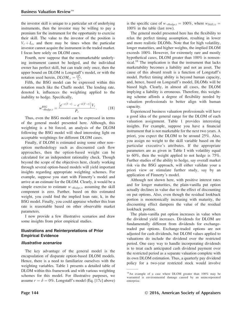
The key advantage of the general model is the

encapsulation of disparate option-based DLOM models.

Hence, there is a need to familiarize ourselves with the

weighting variables. Table 1 presents a detailed table of

DLOM within this framework and with various weighting

schemes for this model. For illustrative purposes, we

assume r ¼ d ¼ 0%. Longstaff’s model (Eq. [17c] above)

is the specific case of w:Hedge;t ¼ 100%, where wSkill;i;t ¼100% in the table (last row).

The general model presented here has the flexibility to

relax the perfect timing assumption, resulting in lower

and more realistic DLOMs. Note that for high volatility,

longer maturities, and higher weights, the implied DLOM

exceeds 100%. However, for extremely rare and mostly

hypothetical cases, DLOM greater than 100% is nonsen-

sical.16 The implication is that the instrument that lacks

marketability becomes a liability and not an asset. The

cause of this absurd result is a function of Longstaff’s

model. Perfect timing ability is beyond human capacity,

and, hence, based on Longstaff’s model, DLOMs will be

biased high. Clearly, in almost all cases, the DLOM

implying a liability is erroneous. Therefore, this weight-

ing scheme affords a degree of flexibility needed by

valuation professionals to better align with human

capacity.

Experienced business valuation professionals will have

a good idea of the general range for the DLOM of each

valuation assignment. Table 1 provides interesting

insights. For example, suppose you have a financial

instrument that is not marketable for the next two years. A

priori, you expect the DLOM to be around 25%. Also,

you assign no weight to the skill variable based on the

particular executive’s attributes. If the appropriate

parameters are as given in Table I with volatility equal

to 60%, then the weight applied to not hedge is 75%.

Further studies of the ability to hedge, say overall market

risk via the BSG approach, will either validate your a

priori view or stimulate further study, say by an

application of Finnerty’s model.

Although not shown here, with positive interest rates

and for longer maturities, the plain-vanilla put option

actually declines in value due to the effect of discounting

on put options. Also, even though the residual lookback

portion is monotonically increasing with maturity, the

discounting effect dampens the value of the residual

lookback portion.

The plain-vanilla put option increases in value when

the dividend yield increases. Dividends for DLOM are

fundamentally different from dividends for exchange-

traded put options. Exchange-traded options are not

adjusted for cash dividends, but DLOM values applied to

valuations do include the dividend over the restricted

period. One easy way to handle incorporating dividends

is to treat each anticipated cash dividend payment over

the restricted period as a separate valuation complete with

its own DLOM estimation. Thus, a quarterly pay dividend

policy for a two-year restricted stock would involve

16An example of a case where DLOM greater than 100% may bewarranted is environmental damage caused by an unincorporatedenterprise.



Tab

le1

Illu

stra

tion

of

the

Gen

eral

Opti

ons-

Bas

edD

LO

MA

ssum

ing

r¼

d¼

0

Vo

lati

lity

(%)

20

40

60

80

20

40

60

80

20

40

60

80

20

40

60

80

20

40

60

80

Yea

rs1

11

12

22

23

33

35

55

51

01

01

01

0

PV

Pu

t($

)7

.97

15

.85

23

.58

31

.08

11

.25

22

.27

32

.86

42

.84

13

.75

27

.10

39

.67

51

.16

17

.69

34

.53

49

.77

62

.89

24

.82

47

.29

65

.72

79

.41

Res

idu

alL

B($

)9

.02

20

.28

34

.01

50

.44

13

.40

31

.46

54

.85

84

.17

17

.03

41

.28

73

.93

11

6.0

42

3.2

95

9.1

91

10

.13

17

8.1

53

6.4

81

00

.23

19

7.4

13

32

.40

w(S

)/w

(NH

)(%

)1

/20

1/4

01

/60

1/8

02

/20

2/4

02

/60

2/8

03

/20

3/4

03

/60

3/8

05

/20

5/4

05

/60

5/8

01

0/2

01

0/4

01

0/6

01

0/8

0

0/0

00

00

00

00

00

00

00

00

00

00

0/2

52

46

83

68

11

37

10

13

49

12

16

61

21

62

0

0/5

04

81

21

66

11

16

21

71

42

02

69

17

25

31

12

24

33

40

0/7

56

12

18

23

81

72

53

21

02

03

03

81

32

63

74

71

93

54

96

0

0/1

00

81

62

43

11

12

23

34

31

42

74

05

11

83

55

06

32

54

76

67

9

25

/02

59

13

38

14

21

41

01

82

96

15

28

45

92

54

98

3

25

/25

49

14

20

61

32

23

28

17

28

42

10

23

40

60

15

37

66

10

3

25

/50

61

32

02

89

19

30

42

11

24

38

55

15

32

52

76

22

49

82

12

3

25

/75

81

72

63

61

22

53

85

31

53

14

86

71

94

16

59

22

86

19

91

43

25

/10

01

02

13

24

41

53

04

76

41

83

75

88

02

44

97

71

07

34

72

11

51

63

50

/05

10

17

25

71

62

74

29

21

37

58

12

30

55

89

18

50

99

16

6

50

/25

71

42

33

31

02

13

65

31

22

74

77

11

63

86

81

05

24

62

11

51

86

50

/50

81

82

94

11

22

74

46

41

53

45

78

42

04

78

01

21

31

74

13

22

06

50

/75

10

22

35

49

15

32

52

74

19

41

67

96

25

55

92

13

63

78

61

48

22

6

50

/10

01

22

64

15

61

83

86

08

52

24

87

71

09

29

64

10

51

52

43

97

16

42

46

75

/07

15

26

38

10

24

41

63

13

31

55

87

17

44

83

13

42

77

51

48

24

9

75

/25

91

93

14

61

32

94

97

41

63

86

51

00

22

53

95

14

93

48

71

64

26

9

75

/50

11

23

37

53

16

35

58

85

20

45

75

11

32

66

21

07

16

54

09

91

81

28

9

75

/75

13

27

43

61

18

40

66

95

23

51

85

12

53

17

01

20

18

14

61

11

19

73

09

75

/10

01

53

14

96

92

14

67

41

06

27

58

95

13

83

57

91

32

19

75

21

22

21

43

29

10

0/0

92

03

45

01

33

15

58

41

74

17

41

16

23

59

11

01

78

36

10

01

97

33

2

10

0/2

51

12

44

05

81

63

76

39

52

04

88

41

29

28

68

12

31

94

43

11

22

14

35

2

10

0/5

01

32

84

66

61

94

37

11

06

24

55

94

14

23

27

61

35

21

04

91

24

23

03

72

10

0/7

51

53

25

27

42

24

88

01

16

27

62

10

41

54

37

85

14

72

25

55

13

62

47

39

2

10

0/1

00

17

36

58

82

25

54

88

12

73

16

81

14

16

74

19

41

60

24

16

11

48

26

34

12

No

te.

w(S

)d

eno

tes

wSk

ill;

i;t,

w(N

H)

den

ote

sw:H

edge;

t,P

VP

ut

den

ote

sth

ep

lain

-van

illa

pu

to

pti

on

mo

del

val

ue,

Res

idu

alL

Bd

eno

tes

the

resi

du

allo

ok

bac

kp

ut

op

tio

np

ort

ion

,an

d

1/2

0d

eno

tes

on

ey

ear

tom

atu

rity

wit

hv

ola

tili

tyo

f2

0.



possibly nine separate calculations (eight dividend

payments and one terminal valuation) that could then be

rolled up into one aggregate valuation and related DLOM.

The general option-based DLOM method presented

here is flexible enough to handle the rich diversity

observed in actual practice while still remaining rather

parsimonious. Specifically, the ability to separate hedging

and investor skill provides a more robust solution to the

DLOM estimation problem. I turn now to reinterpreting

some prior research.

Reinterpreting prior research

Many prior research papers have provided empirical

evidence as illustrations for estimating DLOM. We review

some of this work by reinterpreting their results in light of

the more general model presented herein. The key insight

is that the approach in this paper provides alternative

interpretations for these results. With this alternative

perspective, practitioners can more accurately incorporate

the salient features of their particular DLOM challenge.

Dyl and Jiang (2008) examined Longstaff’s (1995)

model for practical applications. They presented a specific

case study where volatility is given as 60.5%, and

maturity is 1.375 years. Relying on a variety of empirical

sources, they opined that the DLOM should be

approximately 23% and, for the sake of argument,

assume they are correct. As the case study involved an

estate, one would assume wSkill;i;t ¼ 0%. An alternative

interpretation is that w:Hedge;t ¼ 83% would result in the

same 23% DLOM.17 Thus, the general option-based

approach presented here provides a reasonable way to

connect option-based DLOM approaches with other

existing methodologies. Applying these results within

the BSG model implies a loan risk premium of

approximately 4.8%.

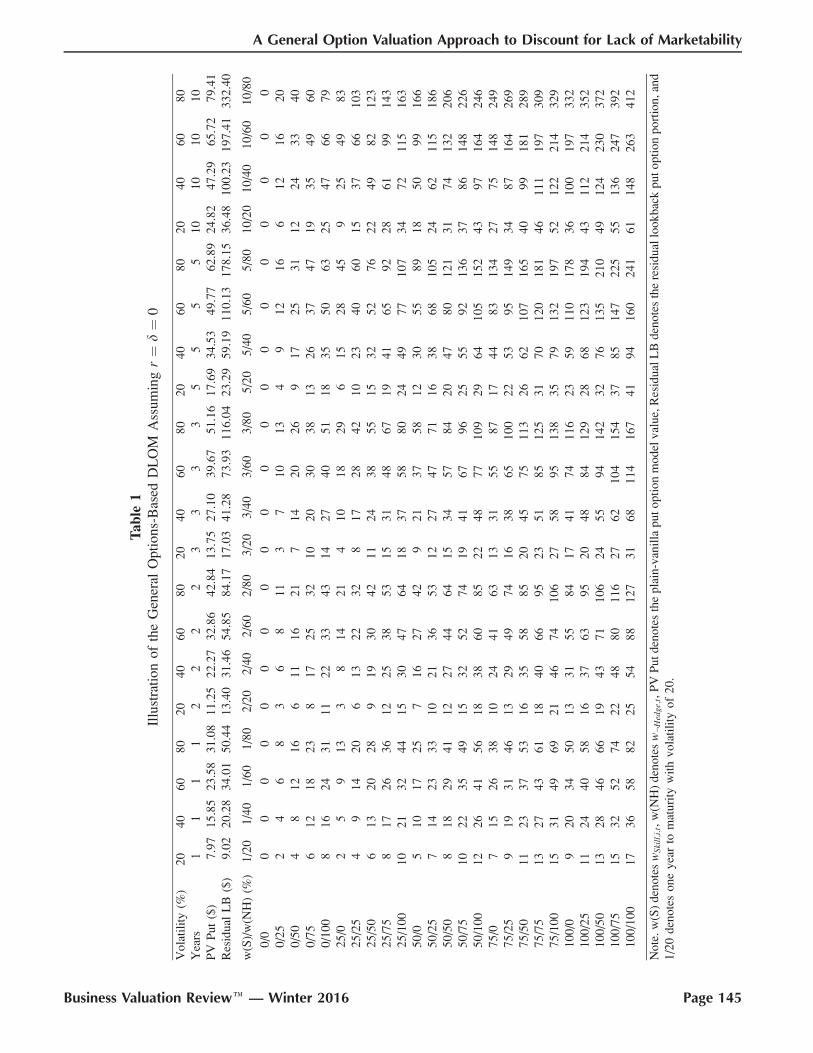
Table 2 presents alternative perspectives on Finnerty’s

(2012) Exhibit 6. Recall Finnerty’s DLOM value cannot

exceed 32.28% due to the volatility time parameter

reaching a maximum of m2ðT � tÞ ¼ lnf2g, while actual

DLOMs are often well in excess of 32.28%. Table 2 is

based on the assumption that DLOM is first driven by the

Table 2An Alternative Interpretation of Mean Implied DLOM

Volatility,

Range (%)

Mean

Implied DLOM

Implied Volatility

(Finnerty)

Implied Maturity

(Finnerty)

Implied Weight,

W(S)

Implied Weight,

\W(:H)

Panel A: Offerings Announced Prior to February 1997

0.0–29.9 19.47% 24.3% 14.3 65.6% 100.0%

30.0–44.9 — — — — —

45.0–59.9 10.51 55.3 0.7 0.0 64.0

60.0–74.9 13.82 62.0 1.0 0.0 40.8

75.0–89.9 24.15 81.1 2.2 0.0 55.7

90.0–104.9 34.97 96.6 þ‘ 0.0 69.2

105.0–120.0 61.51 112.6 þ‘ 2.81 100.0

.120.0 44.10 138.7 þ‘ 0.0 65.5

Average 24.50% 67.5% 3.4 0.0% 66.8%Panel B: Offerings Announced After February 1997

0.0–29.9 12.66% 21.7% 6.8 40.7% 100.0%

30.0–44.9 18.56 33.8 6.7 31.1 100.0

45.0–59.9 15.92 52.3 1.9 0.0 77.2

60.0–74.9 19.21 66.5 1.8 0.0 73.8

75.0–89.9 21.37 82.7 1.6 0.0 66.6

90.0–104.9 21.61 96.5 1.2 0.0 58.3

105.0–120.0 24.89 111.7 1.3 0.0 58.8

.120.0 29.71 146.8 1.4 0.0 55.3

Average 21.31% 73.6% 2.0 0.0% 74.2%

Note. This table is based on Finnerty (2012), Exhibit 6. As I do not have access to the raw data, I assumed the dividend yield was zero.

Mean Implied DLOM is taken directly from Finnerty’s table. Finnerty denotes Finnerty’s model assuming zero dividend yield. From

Finnerty’s table, for each maturity (T¼2, 3, and 4) and Mean Model-Predicted Discount, the implied volatility was estimated. The

average implied volatility of the three maturities is reported as the Implied Volatility (Finnerty). The Implied Maturity is solved such

that the Mean Implied DLOM equals Finnerty’s model based on the estimated implied volatility. W(S) denotes the weight applied to

skill, and W(:H) denotes the weight applied for the portion not hedged.

17We estimate the plain-vanilla put option with r ¼ 0%; d ¼ 0% is equalto $4.21 (the stock price was given at $15.1875). The residual lookbackput portion is $6.48 for a lookback put value of $10.69.



inability to hedge and only then driven by skill. Clearly,

there are many other explanations possible. In only four

cases, skill registered positive values, three of which

occurred with low volatilities. Thus, the evidence

indicates that, in general, the skill weight can safely be

set to zero.18 Thus, Table 2 provides an illustration of the

flexibility of the general option-based model presented

here as well empirical evidence against investor skill.

Conclusions

A general option-based approach to estimating the

DLOM is introduced in this paper. It was demonstrated to

be general enough to address important DLOM challenges,

including restriction period, volatility, hedging availability,

and investor skill. The general option-based DLOM model

was shown to contain the Chaffe model, Longstaff model,

the Finnerty model, and the BSG model as special cases.

The model also contains two weighting variables that

provide valuation professionals much needed flexibility in

addressing the unique challenges of each nonmarketable

valuation assignment. Several prior results were reinter-

preted based on the model presented here.

Acknowledgments

The author gratefully acknowledges the helpful

comments of D. B. H. Chaffe, III, John Stockdale, Jr.,

John M. Griffin, Les Barenbaum, Lance Hall, Brandon N.

Cline, Sang B. Kang, Kate Upton, Pavel Teterin, and

Nicholas Glenn.

References

Abbott, A. 2009. ‘‘Discount for Lack of Marketability:

Understanding and Interpreting Option Models.’’Business Valuation Review 28:144–148.

Abrams, J. B. 2010. Quantitative Business Valuation: AMathematical Approach for Today’s Professional. 2nd

ed. New York: Wiley.

Barenbaum, L., W. Schubert, and K. Garcia. 2015.

‘‘Determining Lack of Marketability Discounts: Em-

ploying an Equity Collar.’’ Journal of EntrepreneurialFinance 17:65–81.

Black, F., and M. Scholes. 1973. ‘‘The Pricing of Options

and Corporate Liabilities.’’ Journal of Political Econ-omy 81:637–654.

Brooks, R., and D. M. Chance. 2014. ‘‘Some Subtle

Relationships and Results in Option Pricing.’’ Journalof Applied Finance 24:94–117.

Brooks, R., D. M. Chance, and B. N. Cline. 2012.

‘‘Private Information and the Exercise of Executive

Stock Options.’’ Financial Management 41:733–764.

Chaffe, D. B. H., III. 1993. ‘‘Option Pricing as a Proxy for

Discount for Lack of Marketability in Private Company

Valuations: A Working Paper.’’ Business ValuationReview, 12 (4)::182–188.

Dyl, E. A., and G. J. Jiang. 2008. ‘‘Valuing Illiquid

Common Stock.’’ Financial Analysts Journal 64:40–

47.

Finnerty, J. 2012. ‘‘An Average-Strike Put Option Model

of the Marketability Discount.’’ Journal of Derivatives41:53–69.

Finnerty, J. 2013a. ‘‘The Impact of Stock Transfer

Restrictions on the Private Placement Discount.’’

Financial Management 42:575–609.

Finnerty, J. 2013b. ‘‘Using Put Option-Based DLOM

Models to Estimate Discounts for Lack of Marketabil-

ity.’’ Business Valuation Review 31:165–170.

Finnerty, J., and R. Park. 2015. ‘‘Collars, Prepaid

Forwards, and the DLOM: Volatility Is the Missing

Link.’’ Business Valuation Review 34:24–30.

Haug, E. G. 2007. The Complete Guide to Option PricingFormulas. 2nd ed. New York: McGraw-Hill.

Internal Revenue Service. 1977. Revenue Ruling 77-287(1977-2 C.B. 319). Available at http://www.aticg.com/

Documents/Revenue/RevRule77-287.pdf, accessed on

June 24, 2015.

Internal Revenue Service. 2009. ‘‘Discount for Lack of

Marketability Job Aid for IRS Valuation Profession-

als.’’ Available at http://www.irs.gov/pub/irs-utl/dlom.

pdf, accessed on June 24, 2015.

Longstaff, F. A. 1995. ‘‘How Much Can Marketability

Affect Security Values?’’ Journal of Finance 50:1767–

1774.

Merton, R. C. 1973. ‘‘Theory of Rational Option

Pricing.’’ Bell Journal of Economics and ManagementScience 4:141–183.

Meulbroek, L. K. 2005. ‘‘Company Stock in Pension

Plans: How Costly Is It?’’ Journal of Law andEconomics 48:443–474.

Pratt, S. P., and A. V. Niculita. 2008. Valuing a Business,The Analysis and Appraisal of Closely Held Business-es. 5th ed. New York: McGraw Hill, Inc.

Seaman, R. M. 2005a. ‘‘Minimum Marketability Dis-

counts—2nd Edition.’’ Business Valuation Review 24

(2):58–64.

Seaman, R. M. 2005b. ‘‘A Minimum Marketability

Discounts.’’ Business Valuation Review 24 (4):177–

180.

Seaman, R. M. 2007. Minimum Marketability Discounts.

3rd ed. Tampa, Flor.: Southland Business Group, Inc.

18One interesting exception may relate to valuation of the generalmanager’s ownership of a successful hedge fund. In this case, ascribingsome weight to skill is in fact warranted, and it is important to have aprebuilt model to handle just such a case.



Seaman, R. M. 2009. Minimum Marketability Discounts.

4th ed. Tampa, Flor.: DLOM, Inc.

Securities and Exchange Commission. 1969. AccountingRelease No. 113. Investment Company Act of 1940Release No. 5847. October 21, 1969. Available at

https://www.sec.gov/rules/interp/1969/ic-5847.pdf, ac-

cessed on June 24, 2015.

Securities and Exchange Commission. 1971. ‘‘Discounts

Involved in Purchases of Common Stock (1966–

1969).’’ In Institutional Investor Study Report of theSecurities and Exchange Commission. Washington,

D.C.: U.S. Government Printing Office, March 10,

Document No. 92-64, Part 5, 2444-2456.

Stockdale, J., Jr. 2013. BVR’s Guide to Discount for Lackof Marketability. 5th ed. Portland, Ore.: Business

Valuation Resources, LLC.

Tabak, D. 2002. ‘‘A CAPM-Based Approach to Calcu-

lating Illiquidity Discounts.’’ NERA Economic Con-

sulting, Working Paper, November 11, 2002. Available

at http://www.nera.com/publications/archive/2002/a-

capmbased-approach-to-calculating-illiquidity-

discounts.html, accessed on June 24, 2015.

Trout, R. R. 2003. ‘‘Minimum Marketability Discounts.’’Business Valuation Review 22:124–126.

Wilmott, P. 2000. Paul Wilmott on Quantitative Finance.

Volume 1. New York: John Wiley & Sons, Ltd.

8 � 2016, American Society of Appraisers


A General Option Valuation Approach to Discount for Lack ...

Documents

Transcript of A General Option Valuation Approach to Discount for Lack ...