Journal of Computational Physics163,349–375 (2000)

doi:10.1006/jcph.2000.6571, available online at http://www.idealibrary.com on

A Gas-Kinetic Scheme for Multimaterial Flowsand Its Application in Chemical Reactions

Y. S. Lian and K. Xu1

Mathematics Department, Hong Kong University of Science and Technology,Clear Water Bay, Kowloon, Hong Kong

E-mail: makxu@uxmail.ust.hk

Received July 19, 1999; revised June 9, 2000

This paper concerns the extension of the multicomponent gas-kinetic BGK-typescheme to chemical reactive flow calculations. In the kinetic model, each componentsatisfies its individual gas-kinetic Bhatnagar–Gross–Krook (BGK) equation, and theequilibrium states of both components are coupled in space and time due to themomentum and energy exchange in the course of particle collisions. At the sametime, according to the chemical reaction rule, one component can be changed intoanother component with a release of energy. The reactant and product may havedifferent ratios of specific heats. The BGK scheme basically uses the collisionalBoltzmann model to mimic the numerical dissipation necessary for shock capturing.The numerical dissipation is controlled by the particle collision pseudo-timeτ . In theresolved viscous calculations, there is a direct relation between the physical viscositycoefficient and the particle collision time. Many numerical test cases presented inthis paper validate the gas-kinetic approach in the application of multicomponentreactive flows. c© 2000 Academic Press

Key Words:gas-kinetic method; multicomponent flow; detonation wave.

1. INTRODUCTION

The development of numerical methods for multimaterial flows has attracted much atten-tion in the last few years [11, 12, 21, 28]. One of the main applications of these methods is tochemical reactive flow [3, 13, 22, 25]. Research in reactive flows, especially those involvingdetonation waves, was pioneered by Zeldovich, von Neumann, and Doering, who developedthe well-known ZND model. The ZND model consists of a nonreactive shock followed bya reaction zone. Since the model was proposed, much theoretical and numerical work onthis problem has been done. Numerical calculation of the ZND detonation was pioneeredby Fickett and Wood [14], who solved the one-dimensional equations using the method of

1 To whom correspondence should be addressed. Fax: (852)2358-1643.

349

0021-9991/00 $35.00Copyright c© 2000 by Academic Press

All rights of reproduction in any form reserved.

350 LIAN AND XU

characteristics in conjunction with a shock fitting method. Longitudinal instability waveswere accurately simulated. Later, Taki and Fujiwara applied van Leer’s upwind method tocalculate two-dimensional traveling detonation waves [31, 33]. They solved the Euler equa-tions coupled with two species equations. The chemical reaction was simulated by a two-stepfinite-rate model and the transverse instabilities around shock front were clearly observed.It was pointed out by Colellaet al. in [7] that if the numerical resolution in the detonativeshock front is not enough, a nonphysical solution can easily be generated. As an example,the solution may have the wrong shock speed. To avoid a nonphysical solution, Engquist andSjogreen [9] used a high-order TVD/ENO numerical method combined with a Runge–Kuttatime marching scheme to solve the combustion problem with special treatment in the shockregion. Around the same time, Kailasanathet al. [20] extended the flux-corrected transport(FCT) algorithm for detonations. In the early 1990s, Bourliouxet al. combined the PPMscheme with conservative front tracking and adaptive mesh refinement in the study of det-onative waves [3–5]. They computed the spatial–temporal structure of unstable detonationin one and two spatial dimensions. Quirk [27] addressed deficiency of the Godunov-typeupwind schemes in solving complex flow problems and suggested a hybrid scheme to sim-ulate the galloping phenomenon in one- and two-dimensional detonations. Recently, Shortand co-workers extensively studied the nonlinear stability of a pulsating detonation wavedriven by a three-step chain-branching reaction [29, 30]. Lindstr¨om [22] analyzed the poorconvergence of the inviscid Euler solutions in the study of detonative waves and suggestedsolving the compressible Navier–Stokes equations directly. Most recently, Hwanget al.[17] pointed out that not only is resolution of the reaction zone important, but also thesize of the computational domain is critical in capturing correct detonative solutions. Sofar, it is well recognized that a good scheme for reactive flow must be able to capture thecorrect shock speed, resolve wave structures in the multidimensional case, and determinethe correct period of the possible unsteady oscillation in the wave.

Ever since the gas-kinetic scheme was proposed for the compressible flow simulations,it has attracted much attention in the CFD community due to its robustness and accuracy.The gas-kinetic schemes are usually catalogued as one group of flux vector splitting (FVS)schemes for hyperbolic equations [15, 32]. Actually, this is not completely true. For ex-ample, in the construction of numerical fluxes, the FVS scheme requires homogeneity ofthe governing equations, such as the Steger–Warming method for the Euler equations. Butthe kinetic method can be directly applied to nonhomogeneity equations, such as the shal-low water equations and hyperbolic–elliptic equations [34, 36]. It can even be applied tothe magnetohydrodynamic equations directly [8, 37], where an exact Riemann solutionis unknown. Besides its generality, the gas-kinetic scheme distinguishes itself from otherschemes by its robustness, especially for high-speed flows with shock and expansion waves.Like many other FVS schemes, the weakness of the collisionless-type kinetic methods isits overdiffusivity. It needs a much refined mesh to get an accurate Navier–Stokes solution.The reason for the overdiffusivity is the underlying free transport mechanism in the kineticmethod. To improve the accuracy of the scheme, the inclusion of particle or pseudo-particlecollisions becomes necessary. This leads directly to the development of the BGK scheme,where the particle collisions are included in the gas evolution process. Mathematically,from the BGK equation, the macroscopic Navier–Stokes equations can be derived [6]. Inother words, for well-resolved flow simulations, the BGK flow solver and the Navier–Stokes solver yield same solutions. Actually, in this situation, any standard central differ-ence scheme is adequate without inclusion of any upwinding or Riemann solver concept.

KINETIC SCHEME FOR REACTIVE FLOW 351

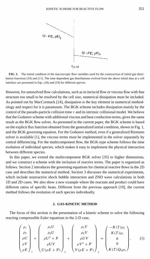
FIG. 1. The initial condition of the macroscopic flow variables used for the construction of initial gas distri-bution functions (10) and (11). The time dependent gas distributions evolved from the above initial data at a cellinterface are presented in Eqs. (18) and (19) for different species.

However, for unresolved flow calculations, such as in inviscid flow or viscous flow with finestructure too small to be resolved by the cell size, numerical dissipation must be included.As pointed out by MacCormack [24], dissipation is the key element in numerical method-ology and respect for it is paramount. The BGK scheme includes dissipation mainly by thecontrol of the pseudo-particle collision timeτ and its intrinsic collisional model. We believethat the Godunov scheme with additional viscous and heat conduction terms, gives the sameresult as the BGK flow solver. As presented in the current paper, the BGK scheme is basedon the explicit flux function obtained from the generalized initial condition, shown in Fig. 1,and the BGK governing equation. For the Godunov method, even if a generalized Riemannsolver is available [1], the viscous terms must be implemented in the solver separately bycentral differencing. For the multicomponent flow, the BGK-type scheme follows the timeevolution of individual species, which makes it easy to implement the physical interactionbetween different species.

In this paper, we extend the multicomponent BGK solver [35] to higher dimensions,and we construct a scheme with the inclusion of reactive terms. The paper is organized asfollows. Section 2 introduces the governing equations for chemical reactive flows in the 2Dcase and describes the numerical method. Section 3 discusses the numerical experiments,which include nonreactive shock bubble interaction and ZND wave calculations in both1D and 2D cases. We also show a new example where the reactant and product could havedifferent ratios of specific heats. Different from the previous approach [19], the currentmethod follows the evolution of each species individually.

2. GAS-KINETIC METHOD

The focus of this section is the presentation of a kinetic scheme to solve the followingreacting compressible Euler equations in the 2-D case,

ρ1

ρ2

ρU

ρV

ρE

t

+

ρ1U

ρ2U

ρU2+ P

ρU V

U (ρE + P)

x

+

ρ1V

ρ2V

ρU V

ρV2+ P

V(ρE + P)

y

=

−K (T)ρ1

K (T)ρ1

00

K (T)Q0ρ1

, (1)

352 LIAN AND XU

whereρ1 is the density of the reactant,ρ2 is the density of the product,ρ = ρ1+ ρ2 isthe total density, andρE is the total energy which includes both kinetic and thermal ones;i.e., ρE = 1

2ρ(U2+ V2)+ P1/(γ1− 1)+ P2/(γ2− 1). HereU , V are the average flow

velocities in thex andy directions, respectively. Each component has its specific heat ratiosγ1 andγ2. P = P1+ P2 is the total pressure, andQ0 is the amount of heat released per unitmass by reaction. The equation of state can be expressed asP1 = ρ1RT andP2 = ρ2RT.K (T) is the chemical reactive rate, which is a function of temperature. The specific formof K (T) will be given in the numerical examples section.

The above reactive flow equations will be solved in two steps. In the first step, thenonreactive gas evolution parts are solved using the multimaterial gas-kinetic method. Inthe second step, the source terms on the right-hand side of Eq. (1) are included in the updateof flow variables inside each cell.

2.1. 2-D Multicomponent BGK Scheme

2.1.1. Gas-kinetic governing equations.The focus of this section is a multicomponentBGK scheme in two dimensions. For the two-dimensional problem, the governing equationfor the time evolution of each component is the BGK model,

f (1)t + u f (1)x + v f (1)y =g(1) − f (1)

τ,

(2)

f (2)t + u f (2)x + v f (2)y =g(2) − f (2)

τ,

where f (1) and f (2) are particle distribution functions for component 1 and 2 gases, andg(1)

andg(2) are the corresponding equilibrium states whichf (1) and f (2) approach. In the aboveequations,τ is the particle collision time, which determines the speed of a nonequilibriumstate approaching an equilibrium one. In the BGK scheme,τ can be regarded as particle col-lision pseudo-time for the unresolved flow calculation; the additional dissipation providedthrough the control of the collision time generates artificial dissipation necessary for shockcapturing. The detailed expression ofτ is given in the section on numerical examples. Therelations between the distribution functions and the macroscopic variables are∫

f (1)φ(1)α d4(1) + f (2)φ(2)α d4(2) = W = (ρ1, ρ2, ρU, ρV, ρE)T , (3)

where

d4(1) = du dv dξ1, d4(2) = du dv dξ2,

φ(1)α =(

1, 0, u, v,1

2

(u2+ v2+ ξ2

1

))T

φ(2)α =(

0, 1, u, v,1

2

(u2+ v2+ ξ2

2

))T

,

are the moments for individual mass, total momentum, and total energy densities. Here,ξ2

1 = ξ21,1+ ξ2

1,2+ · · · + ξ21,K1

andξ22 = ξ2

2,1+ ξ22,2+ · · · + ξ2

2,K2. The integration elements

aredξ1 = dξ1,1 dξ1,2 . . .dξ1,K1 anddξ2 = dξ2,1 dξ2,2 . . .dξ2,K2. K1 andK2 are the degrees

KINETIC SCHEME FOR REACTIVE FLOW 353

of freedom of the internal variablesξ1 andξ2, which are related to the specific heat ratiosγ1 andγ2. For the two-dimensional flow, we have

K1 = (5− 3γ1)/(γ1− 1)+ 1 and K2 = (5− 3γ2)/(γ2− 1)+ 1.

The compatibility condition for the two-component gas mixture is∫ (g(1) − f (1)

)φ(1)α d4(1) + (g(2) − f (2)

)φ(2)α d4(2) = 0, α = 1, 2, 3, 4, 5. (4)

The equilibrium Maxwellian distributionsg(1) andg(2) are generally defined as

g(1) = ρ1(λ1/π)K1+2

2 e−λ1((u−U1)2+(v−V1)

2+ξ21),

g(2) = ρ2(λ2/π)K2+2

2 e−λ2((u−U2)2+(v−V2)

2+ξ22),

whereλ1 andλ2 are functions of temperature. Due to the momentum and energy exchangein particle collisions, the equilibrium statesg(1) and g(2) are assumed to have the samevelocity and temperature at any point in space and time. Therefore, from the given initialmacroscopic variables at any point in space and time,

W(1) =∫

g(1)φ(1)α d4(1) = (ρ1, ρ1U1, ρ1V1, ρ1E1)T ,

W(2) =∫

g(2)φ(2)α d4(2) = (ρ2, ρ2U2, ρ2V2, ρ2E2)T ,

we can get the corresponding equilibrium values

W(1) =(ρ1, ρ1U, ρ1V,

1

2ρ1

(U2+ V2+ K1+ 2

2λ

))T

,

(5)

W(2) =(ρ2, ρ2U, ρ2V,

1

2ρ2

(U2+ V2+ K2+ 2

2λ

))T

,

where the equilibrium valuesU , V , andλ can be obtained from the mass, momentum, andenergy conservation,

ρ = ρ1+ ρ2,

ρ1U1+ ρ2U2 = ρU,

ρ1V1+ ρ2V2 = ρV,

ρ1E1+ ρ2E2 = ρ(U2+ V2)

2+ (K + 2)ρ

4λ.

(6)

With the definition of “averaged” value of internal degrees of freedomK ,

K = ρ1K1+ ρ2K2

ρ,

and the corresponding specific heat ratioγ ,

γ = K + 4

K + 2,

354 LIAN AND XU

the valuesU , V , andλ can be obtained from Eq. (6) explicitly,

U = ρ1U1+ ρ2U2

ρ,

V = ρ1V1+ ρ2V2

ρ,

and

λ = 1

4

(K + 2)ρ

ρ1E1+ ρ2E2− 12ρ(U

2+ V2).

As a result, the equilibrium states can be expressed as

g(1) = ρ1(λ/π)K1+2

2 e−λ((u−U )2+(v−V)2+ξ21),

g(2) = ρ2(λ/π)K2+2

2 e−λ((u−U )2+(v−V)2+ξ22).

The governing equations (2) are closely related to the viscous governing equations, and thedissipative coefficients are proportional to the collision timeτ [34].

2.1.2. Multicomponent gas-kinetic scheme.Numerically, the Boltzmann equations (2)are solved using a splitting method. For example, in thex direction, we solve

f (1)t + u f (1)x =g(1) − f (1)

τ,

f (2)t + u f (2)x =g(2) − f (2)

τ,

and in they direction,

f (1)t + v f (1)y =g(1) − f (1)

τ,

f (2)t + v f (2)y =g(2) − f (2)

τ.

In each fractional step, the compatibility condition (4) is still satisfied.For the BGK model, in thex direction the integral solution off at a cell interfacexi+1/2

and timet is

f (1)(xi+1/2, t, u, v, ξ1

) = 1

τ

∫ t

0g(1)(x′, t ′, u, v, ξ1)e

−(t−t ′)/τ dt′

+ e−t/τ f (1)0

(xi+1/2− ut

)(7)

for component 1 and

f (2)(xi+1/2, t, u, v, ξ2

) = 1

τ

∫ t

0g(2)(x′, t ′, u, v, ξ2)e

−(t−t ′)/τ dt′

+ e−t/τ f (2)0

(xi+1/2− ut

)(8)

for component 2, wherexi+1/2 is the location of the cell interface andx′ = xi+1/2− u(t − t ′)is the particle trajectory. There are four unknowns in Eq. (7) and Eq. (8). Two of them are

KINETIC SCHEME FOR REACTIVE FLOW 355

initial gas distribution functionsf (1)0 and f (2)0 at the beginning of each time stept = 0, andthe others areg(1) andg(2) in both space and time locally around(xi+1/2, t = 0).

Numerically, at the beginning of each time stept = 0, we have the macroscopic flowdistributions inside each celli ,

Wi = (ρ1, ρ2, ρU, ρV, ρE)Ti .

From the discretized initial data, we can apply the standard van Leer limiterL(·, ·) tointerpolate the conservative variablesWi and get the reconstructed initial data

Wi (x) = Wi + L(si+, si−)(x − xi ), for x ∈ [xi−1/2, xi+1/2], (9)

where(Wi (xi−1/2), Wi (xi+1/2)) are the reconstructed point-wise values at the cell interfacesxi−1/2 andxi+1/2 in cell i .

To simplify the notation, in the followingxi+1/2 = 0 is assumed. With the interpolatedmacroscopic flow distributionsWi , the initial distribution functionsf (1)0 and f (2)0 in Eq. (7)and Eq. (8) can be constructed as

f (1)0 ={(

1+ a(1)l x)g(1)l , x< 0,(

1+ a(1)r x)g(1)r , x> 0,

(10)

for component 1 and

f (2)0 ={(

1+ a(2)l x)g(2)l , x< 0,(

1+ a(2)r x)g(2)r , x> 0,

(11)

for component 2. The corresponding macroscopic variables for each component aroundthe cell interface are shown in Fig. 1. The equilibrium states in Eq. (7) and Eq. (8) around(x = 0, t = 0) are assumed to be

g(1) = (1+ (1− H(x))a(1)l x + H(x)a(1)r x + A(1)t)g(1)0 , (12)

and

g(2) = (1+ (1− H(x))a(2)l x + H(x)a(2)r x + A(2)t)g(2)0 , (13)

where H(x) is the Heaviside function.g(1)0 andg(2)0 are the initial equilibrium states locatedat the cell interface,

g(1)0 = ρ1,0(λ0/π)K1+2

2 e−λ0((u−U0)2+(v−V0)

2+ξ21),

g(2)0 = ρ2,0(λ0/π)K2+2

2 e−λ0((u−U0)2+(v−V0)

2+ξ22).

(14)

The parametersa(1,2)l ,r , a(1,2)l ,r , and A(1,2) are from the Taylor expansion of the equilibriumstates and have the forms

a(1,2)l = a(1,2)l ,1 + a(1,2)l ,2 u+ a(1,2)l ,3 v + a(1,2)l ,4

u2+ v2+ ξ2(1,2)

2,

a(1,2)r = a(1,2)r,1 + a(1,2)r,2 u+ a(1,2)r,3 v + a(1,2)r,4

u2+ v2+ ξ2(1,2)

2,

356 LIAN AND XU

a(1,2)l = a(1,2)l ,1 + a(1,2)l ,2 u+ a(1,2)l ,3 v + a(1,2)l ,4

u2+ v2+ ξ2(1,2)

2,

a(1,2)r = a(1,2)r,1 + a(1,2)r,2 u+ a(1,2)r,3 v + a(1,2)r,4

u2+ v2+ ξ2(1,2)

2,

A(1,2) = A(1,2)1 + A(1,2)2 u+ A(1,2)3 v + A(1,2)4

u2+ v2+ ξ2(1,2)

2.

All coefficientsa(1,2)l ,1 ,a(1,2)l ,2 , . . . , A(1,2)4 are local constants. To determine all these unknowns,the BGK scheme is summarized as follows.

The equilibrium Maxwellian distribution functions located on the left side of the cellinterfacexi+1/2 for components 1 and 2 are

g(1)l = ρ1,l (λl/π)K1+2

2 e−λl ((u−Ul )2+(v−Vl )

2+ξ21),

and

g(2)l = ρ2,l (λl/π)K2+2

2 e−λl ((u−Ul )2+(v−Vl )

2+ξ22). (15)

At the locationx = 0, the relations (3) and (4) require

Wi(xi+1/2

) ≡

ρ1,i

ρ2,i

(ρU )i

(ρV)i

(ρE)i

xi+1/2

=∫

g(1)l φ1α d4(1) + g(2)l φ2

α d4(2) =

ρ1,l

ρ2,l

(ρU )l

(ρV)l

(ρE)l

,

and

Wi+1(xi+1/2

) ≡

ρ1,i+1

ρ2,i+1

(ρU )i+1

(ρV)i+1

(ρE)i+1

xi+1/2

=∫

g(1)r φ(1)α d4(1) + g(2)r φ(2)α d4(2) =

ρ1,r

ρ2,r

(ρU )r(ρV)r(ρE)r

,

from which we have

ρ1,l

ρ2,l

Ul

Vl

λl

=

ρ1,i

ρ2,i

U i

V i

(K1+ 2)ρ1,i + (K2+ 2)ρ2,i

4((ρE)i − 1

2 ρ i (U2i + V2

i ))

xi+1/2

.

KINETIC SCHEME FOR REACTIVE FLOW 357

Similarly,

ρ1,r

ρ2,r

Ur

Vr

λr

=

ρ1,i+1

ρ2,i+1

U i+1

V i+1

(K1+ 2)ρ1,i+1+ (K2+ 2)ρ2,i+1

4((ρE)i+1− 1

2 ρ i+1(U2i+1+V2

i+1))

xi+1/2

.

Therefore,g(1)l , g(2)l , g(1)r , andg(2)r are totally determined.Sinceg(1) andg(2) have the same temperature and velocity at any point in space and time,

as shown in Eq. (5), the parameters(a(1,2)l ,1 ,a(1,2)l ,2 ,a(1,2)l ,3 ,a(1,2)l ,4 ) are not totally independent.

Sincea(1,2)l ,2 ,a(1,2)l ,3 , anda(1,2)l ,4 depend only on derivatives ofU0, V0, andλ0, the requirementof common velocity and temperature in space and time gives

al ,2 ≡ a(1)l ,2 = a(2)l ,2 , al ,3 ≡ a(1)l ,3 = a(2)l ,3 , and al ,4 ≡ a(1)l ,4 = a(2)l ,4 .

This is also true among the parametersa(1)r,2,a(2)r,2, . . . ,a

(1)r,2,a

(2)r,2 on the right-hand side of a

cell interface. Therefore, for each celli , we have

Wi(xi+1/2

)− Wi (xi )

xi+1/2− xi≡

ω1

ω2

ω3

ω4

ω5

=∫ (

a(1)l ,1 +al ,2u+al ,3v+al ,4u2+ v2+ ξ2

1

2

)g(1)l φ(1)α d4(1)

+(

a(2)l ,1 +al ,2u+al ,3v+al ,4u2+ v2+ ξ2

2

2

)g(2)l φ(2)α d4(2). (16)

The above five equations uniquely determine the five unknowns(a(1)l ,1 ,a(2)l ,1 ,al ,2,al ,3,al ,4)

and the solutions are the following: Define

51 = ω3−Ul (ω1+ ω2),

52 = ω4− Vl (ω1+ ω2),

53 = ω5−U2

l + V2l + K1+2

2λl

2ω1− U2

l + V2l + K2 + 2

2λl

2ω2.

The solutions of Eq. (16) are

al ,4 = 8λ2l (53−Ul51− Vl52)

(K1+ 2)ρ1,l + (K2+ 2)ρ2,l,

al ,3 = 2λl

ρ1,l + ρ2,l

(52− (ρ1,l + ρ2,l )Vl

2λlal ,4

),

al ,2 = 2λl

ρ1,l + ρ2,l

(51− (ρ1,l + ρ2,l )Ul

2λlal ,4

),

358 LIAN AND XU

a(2)l ,1 =1

ρ2,l

(ω2− ρ2,l (Ul al ,2+ Vl al ,3)− ρ2

(U2

l + V2l

2+ K2+ 2

4λl

)al ,4

),

a(1)l ,1 =1

ρ1,l

(ω1− ρ1,l (Ul al ,2+ Vl al ,3)− ρ1

(U2

l + V2l

2+ K1+ 2

4λl

)al ,4

).

With the same method, all terms ina(1,2)r terms can be obtained.By taking the limit of(t → 0) in Eq. (7) and Eq. (8), applying the compatibility condition

at (x = xi+1/2, t = 0), and using Eqs. (10) and (11), we get

(ρ1,0, ρ2,0, ρ0U0, ρ0V0, ρ0E0)T

≡∫

g(1)0 φ(1)α d4(1) + g(2)0 φ(2)α d4(2)

= limt→0

e−t/τ∫

f (1)0

(xi+1/2− ut

)φ(1) d4(1) + f (2)0

(xi+1/2− ut

)φ(2) d4(2)

=∫ (

H(u)g(1)l + (1− H(u))g(1)r

)φ(1)α d4(1) + (H(u)g(2)l + (1− H(u))g(2)r

)φ(2)α d4(2).

(17)

The right-hand side of the above equation can be evaluated explicitly usingg(1,2)l ,r in Eq. (15).Therefore,ρ1,0, ρ2,0, λ0, U0, andV0 in Eq. (14) can be obtained by solving Eq. (17). As aresult,g(1)0 andg(2)0 are determined. Then, connecting the macroscopic variables

W0 = (ρ1,0, ρ2,0, ρ0U0, ρ0V0, ρ0E0)T

at the cell interface with the cell-centered values in Eq. (9) on both sides, we get the slopesfor the macroscopic variables,

W0− Wi (xi )

xi+1/2− xi, and

Wi+1(xi+1)−W0

xi+1− xi+1/2,

from which a(1)l anda(1)l in Eq. (12) anda(2)r anda(2)r in Eq. (13) can be determined usingthe same techniques for solving Eq. (16). At this point, there are only two unknownsA(1,2)

left for the time evolution parts of the gas distribution functions in Eq. (12) and Eq. (13).Substituting Eq. (10), Eq. (11), Eq. (12), and Eq. (13) into the integral solutions Eq. (7) and

Eq. (8), we get

f (1)(xi+1/2, t, u, v, ξ1

) = (1− e−t/τ)g(1)0 + τ

(t/τ − 1+ e−t/τ

)A(1)g(1)0

+ (τ(−1+ e−t/τ)+ te−t/τ

)(a(1)l H(u)+ a(1)r (1− H(u))

)ug(1)0

+ e−t/τ((

1− uta(1)l

)H(u)g(1)l +

(1− uta(1)r

)(1− H(u))g(1)r

),

(18)

and

f (2)(xi+1/2, t, u, v, ξ2

) = (1− e−t/τ)g(2)0 + τ

(t/τ − 1+ e−t/τ

)A(2)g(2)0

+ (τ(−1+ e−t/τ)+ te−t/τ

)(a(2)l H[u] + a(2)r (1− H(u))

)ug(2)0

+ e−t/τ((

1− uta(2)l

)H(u)g(2)l +

(1− uta(2)r

)(1− H(u))g(2)r

).

(19)

KINETIC SCHEME FOR REACTIVE FLOW 359

To evaluate the unknownsA(1,2) in the above two equations, we can use the compatibilitycondition at the cell interfacexi+1/2 over the whole CFL time step1t ,

∫ 1t

0

∫ (g(1) − f (1)

)φ(1)α d4(1) dt + (g(2) − f (2)

)φ(2)α d4(2) dt = 0,

from which we can get

∫g(1)0 A(1)φ(1)α d4(1) + g(2)0 A(2)φ(2)α d4(2)

=∫ (

A(1)1 + A2u+ A3v + A4u2+ v2+ ξ2

1

2

)g(1)0 φ(1)α d4(1)

+(

A(2)1 + A2u+ A3v + A4u2+ v2+ ξ2

2

2

)g(2)0 φ(2)α d4(2)

= 1

γ0

∫ [γ1g(1)0 + γ2u

(a(1)l H(u)+ a(1)r (1−H(u))

)g(1)0 + γ3

(H(u)g(1)l + (1−H(u))g(1)r

)+ γ4u

(a(1)l H(u)g(1)l + a(1)r (1− H(u))g(1)r

)]φ(1)α d4(1) + [γ1g(2)0 + γ2u

(a(2)l H(u)

+ a(2)r (1− H(u)))g(2)0 + γ3

(H(u)g(2)l + (1− H(u))g(2)r

)+ γ4u(a(2)l H(u)g(2)l

+a(2)r (1− H(u))g(2)r

)]φ(2)α d4(2), (20)

where

γ0 = 1t − τ(1− e−1t/τ),

γ1 = −(1− e−1t/τ

),

γ2 = −1t + 2τ(1− e−1t/τ

)−1te−1t/τ ,

γ3 =(1− e−1t/τ

),

and

γ4 = −τ(1− e−1t/τ

)+1te−1t/τ .

The right-hand side of Eq. (20) is known; therefore all parameters inA(1,2) terms can beobtained explicitly.

Finally the time-dependent numerical fluxes for component 1 and component 2 gasesacross a cell interface can be obtained by taking the moments of the individual gas distri-bution functionsf (1) and f (2) in Eq. (18) and Eq. (19) separately, which are

Fρ1

0

Fρ1U1

Fρ1V1

Fρ1E1

i+1/2

=∫

uφ(1)α f (1)(xi+1/2, t, u, v, ξ1

)d4(1),

360 LIAN AND XU

and 0Fρ2

Fρ2U2

Fρ2V2

Fρ2E2

i+1/2

=∫

uφ(2)α f (2)(xi+1/2, t, u, v, ξ2

)d4(2).

Integrating the above time-dependent flux functions in a whole time step1t , we can getthe total mass, momentum, and energy transports for each component, from which the flowvariables in each cell can be updated.

In comparison with traditional central schemes and popular Riemann solvers, the eval-uation of the gas distributions in Eqs. (18) and (19) is relatively expensive. However, boththe viscous effect and the coupling of the spatial and temporal gas evolution are includedin these distribution functions. Therefore, in a certain sense, the BGK method gives a moreaccurate representation of the flow motion under a more generalized initial condition, i.e.,the inclusion of slopes at the left- and right-hand sides of a cell interface; see Fig. 1. If onlyinviscid flux functions are required, the distribution functions can be simplified to

f (1)(xi+1/2, t, u, v, ξ1

) = (1− e−t/τ)g(1)0 + e−t/τ

(H(u)g(1)l + (1− H(u))g(1)r

),

and

f (2)(xi+1/2, t, u, v, ξ1

) = (1− e−t/τ)g(2)0 + e−t/τ

(H(u)g(2)l + (1− H(u))g(2)r

).

This simplified formulation has been applied to the MHD simulation [37].

2.2. Reaction Step and Flow Update

After obtaining the flux functions across a cell interface, we need to solve an ODE toaccount for the source term, i.e.,Wt = S. More specifically, inside each cell we need tosolve

(ρ1)t = −K (T)ρ1,

(ρ2)t = K (T)ρ1,

(ρE)t = K Q0ρ1.

(21)

In the current study, one step forward-Euler method is used to solve the above equations.In summary, the update of the flow variables inside cell(i, j ) from stepn to n+ 1 is

through the formulation

Wn+1i, j = Wn

i, j +1

1V

(1y∫ 1t

0

(Fi−1/2, j − Fi+1/2, j

)dt

+1x∫ 1t

0

(Gi, j−1/2− Gi, j+1/2

)dt

)+1t Si, j ,

whereSi, j is the corresponding source term in cell(i, j ), F andG are numerical fluxes acrosscell interfaces by solving the multicomponent BGK equations, and1V is the area of thecell (i, j ). We have also tried a second-order Runge–Kutta time stepping method to update

KINETIC SCHEME FOR REACTIVE FLOW 361

the source term. It is observed that there is basically no difference in the simulation resultsbetween using first- and second-order time stepping schemes for the test cases presented inthe next section.

3. NUMERICAL EXAMPLES

In this section, we test the multicomponent BGK scheme for both nonreactive and reactiveflows. For the viscous calculations, the collision timeτ in the BGK scheme presented inthe last section is set to be

τ = µ/P,

whereµ is the dynamical viscosity coefficient andP is the total local pressure. For theviscous flow,µ is a fixed number. In the mesh-refinement study of the viscous flow cal-culation, the simulation results can be convergent only after the physical viscosity takes adominant role and the physical structure can be well resolved by the mesh size. The con-vergence study of the BGK scheme for the Rayleigh–Taylor case is presented in [19]. Thekinetic BGK method is actually a mesoscopic model rather than a microscopic model forthe flow description. The collision timeτ cannot take the real particle collision time, suchas 10−9 s for the molecular collisions in the air, because it is impossible to get such a refinedmesh size and time step to resolve individual particle collision. In the BGK scheme forthe Navier–Stokes solution, the collision time is solely determined from the macroscopicviscosity coefficient.

For the inviscid flow calculations, the collision time is defined as

τ = 0.051t + |Pl − Pr |Pl + Pr

1t,

where1t is the CFL time step, andPl andPr are the corresponding pressure in the statesgl andgr of the initial gas distribution functionf0. With the above definition, the numericaldissipation will be reduced along with the mesh refinement. In the smooth flow region,the above expression gives about 20 collisions inside each time step. In other words, themagnitude of corresponding numerical diffusion is about 1/10 of that in the kinetic fluxvector splitting (KFVS) scheme [23, 26, 34]. In the discontinuous region, the collision timewill be close to the time step in order to provide enough dissipation to construct a numericaldiscontinuity jump. Whatever the collision time, numerical dissipation always exist in theBGK scheme and is consistent with the Navier–Stokes dissipative terms. In other words,the BGK scheme gives an approximate solution under the generalized initial condition(Fig. 1) for the viscous governing equations, and the viscosity coefficient is controlled bythe particle collision pseudo-time. Starting from the Godunov method, it is equivalent toconstruct a generalized Riemann solution for the viscous governing equations. Also, thecurrent approach is more robust than the previous “single component” kinetic method forthe reactive flows [19]. The detail comparison is given in [18].

For the chemical reactive flow, if the flow structure is not well resolved by the meshsize, the current BGK scheme cannot get grid-independent solutions. It is true for any othershock capturing scheme applied to the reactive flows. As realized by Lindstorm [22], toobtain grid-independent solutions, a large amount of physical viscosity must be added inthe flow simulations. The BGK scheme does it through the inclusion of large collision time,such as the case (5) in the reactive flow calculation section.

362 LIAN AND XU

FIG. 2. Physical domain for shock–bubble interaction.

3.1. Nonreactive Multimaterial Flow Calculations

In this section, we show two cases of shock–bubble interactions. The main differencesbetween these two cases are the specific heat ratios and the initial gas densities inside thebubble with respect to the density of the outside air. The density difference yields differentflow patterns around the material interface after its interaction with the shock.

Case (1): A Ms =1.22 shock wave in air hits a helium cylindrical bubble.We examinethe interaction of aMs = 1.22 planar shock wave, moving in the air, with a cylindrical heliumbubble. Experimental data can be found in [16] and numerical solutions using adaptive meshrefinement have been reported in [28]. Recently, a ghost fluid method has been applied tothis case too [11]. A schematic description of the computational setup is shown in Fig. 2,where reflection boundary conditions are used on the upper and lower boundaries. The initialflow distribution is determined from the standard shock relation with the given strength ofthe incident shock wave. The bubble is assumed to be in both thermal and mechanicalequilibrium with the surrounding air. The nondimensionalized initial conditions are

W = (ρ = 1,U = 0,V = 0, P = 1, γ = 1.4) preshock air

W = (ρ = 1.3764,U = −0.394,V = 0, P = 1.5698, γ = 1.4) postshock air

W = (ρ = 0.1358,U = 0,V = 0, P = 1, γ = 1.67) helium.

The nondimensional cell size used in the computation is1x = 1y = 0.25.To identify weak flow features which are often lost within contour plots, we present a

number of numerical Schlieren images. These pictures depict the magnitude of the gradientof the density field

|1ρ| =√(

∂ρ

∂x

)2

+(∂ρ

∂y

)2

, (22)

and hence they may be viewed as idealized images; the darker the image, the larger thegradient. The density derivatives are computed using straightforward central-differencing.The following nonlinear shading functionφ is used to accentuate weak flow features [28],

φ = exp

(−k|1ρ||1ρ|max

), (23)

wherek is a constant which takes the value 10 for helium and 60 for air. For the Refrigerant22 (R22) simulation in the next test case, we use 1 for heavy fluid and 80 for air.

KINETIC SCHEME FOR REACTIVE FLOW 363

FIG. 4. The density profiles along the centerline for the shock-Helium interaction case at timet = 125.0.(a) Density of air, (b) density of Helium, and (c) total density.

Figure 3 shows snapshots of numerical Schlieren-type images at nondimensional timest = 0.0 andt = 125.0. Before the shock hits the bubble, wiggles usually appear around thebubble because the numerical scheme cannot precisely keep the sharp material interface.The wiggles spread in all directions. When they reach the solid wall, they bounce back. Butall these noises have a very small magnitude. After the shock hits the bubble, the originalshock wave separates into a reflected and a transmitted shock wave. A complex pattern ofdiscontinuities has formed around the top and bottom of the bubble. Figure 4 shows thedensity distributions around the central line at timet = 125.0. There are approximately10 points around the material interface, which is much wider than those obtained fromschemes with special treatment at the material interfaces [11, 21]. In other words, thekinetic scheme always has an intrinsic dissipative term, and it is impossible to keep a verysharp interface. A similar phenomenon takes place in the 1D case [1]. Since helium hasa lower density than air, any small perturbation at the material interface can be amplifiedto form the interface instability. This instability at the material interface is closely relatedto the Richtmyer–Meshkov instability. In comparison with the result in [11], the currentscheme could capture the unstable interface structure automatically, and the result here isqualitatively consistent with both the experiment and that from the mesh-refinement study[28]. It is a common practice that many schemes with special treatments at the materialinterface could easily remove the interface instability. So, it is an interesting problem tofurther study the shock–bubble interaction case and to understand the dynamics of anyspecial numerical treatment on the interface stability. In our calculations, the stable andunstable interfaces are captured automatically.

364 LIAN AND XU

FIG. 3. Numerical Schlieren images of the interaction between aMs = 1.22 shock wave in the air and ahelium cylindrical bubble. The shock is moving from right to left. The second image describes the fields of thedensity gradient distribution at timet = 125.0, where the red corresponds to one material and the blue to anotherone.

FIG. 5. Numerical Schlieren images of the interaction between aMs = 1.22 shock wave and a R22 cylindricalbubble. The second image describes the fields of the density gradient distribution at timet = 150.0, where the redcolor represents one material and the blue color another one.

KINETIC SCHEME FOR REACTIVE FLOW 365

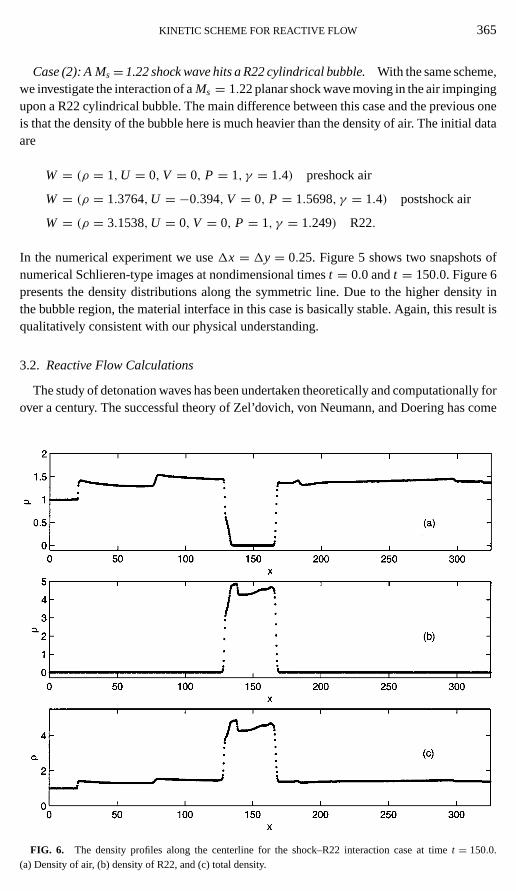
Case (2): A Ms= 1.22 shock wave hits a R22 cylindrical bubble.With the same scheme,we investigate the interaction of aMs = 1.22 planar shock wave moving in the air impingingupon a R22 cylindrical bubble. The main difference between this case and the previous oneis that the density of the bubble here is much heavier than the density of air. The initial dataare

W = (ρ = 1,U = 0,V = 0, P = 1, γ = 1.4) preshock air

W = (ρ = 1.3764,U = −0.394,V = 0, P = 1.5698, γ = 1.4) postshock air

W = (ρ = 3.1538,U = 0,V = 0, P = 1, γ = 1.249) R22.

In the numerical experiment we use1x = 1y = 0.25. Figure 5 shows two snapshots ofnumerical Schlieren-type images at nondimensional timest = 0.0 andt = 150.0. Figure 6presents the density distributions along the symmetric line. Due to the higher density inthe bubble region, the material interface in this case is basically stable. Again, this result isqualitatively consistent with our physical understanding.

3.2. Reactive Flow Calculations

The study of detonation waves has been undertaken theoretically and computationally forover a century. The successful theory of Zel’dovich, von Neumann, and Doering has come

FIG. 6. The density profiles along the centerline for the shock–R22 interaction case at timet = 150.0.(a) Density of air, (b) density of R22, and (c) total density.

366 LIAN AND XU

to be a standard model. The ZND solution for the reacting compressing Euler equations isdescribed in [13]. It consists of a nonreactive shock followed by a reaction zone; both theshock and the reaction zone travel at a constant speedD. Given the specific heat ratioγand the heat releaseQ0, there is a minimum shock speed, the so-called Chapman–Jouguetvalue,DCJ, above which the ZND solution can be constructed.

The parameter that relates the shock speedD of a given detonation wave to the CJ velocityDCJ is the overdrive factorf , which is defined as

f ≡(

D

DCJ

)2

. (24)

The value off is one of the factors that determine the stability of the detonative front.In the following test cases, we only consider reactive flows with two species, i.e., a reactant

and a product. The reactant is converted to the product by a one-step irreversible reactiverule governed by Arrhenius kinetics. The factorK (T), which depends on the temperature,is given by

K (T) = K0Tαe−E+/T ,

whereK0 is a positive constant andE+ is the activation energy. In the current paper, weassume thatα = 0 and the gas constantR is normalized to unity. Therefore, the abovetemperatureT is determined byT = P/ρ.

One important parameter in the numerical calculation of ZND solution is the half-reactionlength L1/2, which is defined as the distance for half-completion of the reactant startingfrom the shock front. Usually the reaction prefactorK0 is selected so that the half-reactionlength is unity. From the Arrhenius formula, the half-reaction length is defined as

L1/2 =∫ 1/2

1

D −U

K0Z exp(−E+/T)d Z, (25)

whereD is the speed of the shock, andU is the postshock flow speed.In the output of numerical results, the mass fractionZ is defined as

Z = ρ1

ρ1+ ρ2.

Case (1): 1-D stable ZND detonation:γ = 1.2, Q0= 50, E+ = 50.0, f= 1.8. This testcase is from [3]. The preshock state is normalized toP0 = ρ0 = 1 and velocityU0 = V0 = 0,and the postshock can be obtained using the Chapman–Jouguet condition. The prefactorK0

is chosen to beK0 = 145.68913 so that the length of the half-reaction zoneL1/2 is unity.This case corresponds to the stable ZND profile. The results with 10, 20, and 40 points/L1/2

are shown in Figs. 7 and 8.

Case (2): 1-D unstable detonation:γ = 1.2, Q0= 50, E+ = 50, f = 1.6. To obtaina high-quality simulation result for the unstable overdriven detonation, a high-resolutionsolution is usually required to resolve the instability. At the same time, the correct capturingof oscillatory period requires a large computational domain. As pointed out in [17], for aparticular computation, one may be tempted to keep only a few points behind the shock,with the reasoning that the information behind the shock either never catches up with or

KINETIC SCHEME FOR REACTIVE FLOW 367

FIG. 7. Mesh refinement study of the pressure history at the shock front for the stable detonation wave, wheref = 1.8, γ = 1.2, Q0 = E+ = 50, andL1/2 = 1.0 (CFL= 0.5).

FIG. 8. Numerical solutions (solid lines) of densityρ, velocity U, pressure P and mass fraction Z, wheref = 1.8, γ = 1.2, Q0 = E+ = 50, L1/2 = 1.0, and 10 points/L1/2 (CFL= 0.5). The dash lines are the exactsolutions.

368 LIAN AND XU

does not affect the shock during the computation. However, if too small a computationaldomain behind the shock is specified, the points at the edge of and outside the computationaldomain cease to be updated after some time, leading to corruption of the data in that region.TheU + c waves emanating from an inappropriate boundary condition eventually catch upwith the shock itself and alter the shock properties erroneously. The analysis in [17] showsthat if one expects the numerical results at timet to be correct, the computational domainL andt must satisfy the inequality

t <L

U + c− D+ L

D, (26)

whereU is the speed of the postshock flow, andc is the sound speed. For the current test,L should satisfy

L ≥ 1.88t.

This classical unstable detonation wave was first studied by Fickett and Wood [14]. Animportant physical quality for unstable detonation is the pressure history at the precursorshock in the oscillatory ZND wave as a function of time. For a stable ZND wave, thisshock pressure history should exhibit small fluctuations about the known precursor shockvalue and decay as time evolves. In the case of unstable detonations, the shock front pres-sure history makes larger excursions from the ZND value. For the caseγ = 1.2, q0 = 50,E+ = 50, and overdrivef = 1.6, according to Erpenbeck [10] this ZND profile is a regularperiodic pulsating detonation with a maximum shock pressure given by 101.1± 0.2 whilethe unperturbed ZND shock pressure is 67.3.

In the current study, the density and pressure are normalized to unity after the shock. SinceQ0 = 50, γ = 1.2, the CJ speed becomesDCJ = 6.80947, and the prefactor is chosen to beK0 = 230.75 to get a unit half-reaction length. The postshock state can be determined by theChapman–Jouguet condition with the given shock speed. Due to the “start-up” numericalincompatibility, there is a large initial shock pressure up to 114 at timet equal to 8; seeFig. 9. Aftert > 15, the motion of the shock front becomes periodic.

In this test, we observe that at least 20 points/L1/2 are needed for a correct unstableZND solution. In Figs. 9 and 10 we show the numerical results with 20 points/L1/2 and40 points/L1/2, respectively. At the same time, the result with 80 points/L1/2 is given as areference. In Table I, the data of local maximum and minimum pressure as a function oftime are listed.

Case (3): Weak shock wave hitting the reactant.To validate the multicomponent BGKscheme, we design the following 1D case to simulate the chemical reaction in which thereactant and product have different specific heat ratiosγ . The initial condition is

WL = (ρL ,UL , PL , γL) = (2.667, 1.479, 4.500, 1.4) postshock air

WM = (ρM ,UM , PM , γM) = (1.0, 0.0, 1.0, 1.4) preshock air

WR = (ρR,UR, PR, γR) = (0.287, 0.0, 1.0, 1.2) (reactant).

This is a case of a weak shock wave withM = 2.0 hitting the reactant. We use the Arrheniusform for the reaction rate withE+ = Q0 = 50 andK0 = 600.0. The numerical cell size is

KINETIC SCHEME FOR REACTIVE FLOW 369

FIG. 9. Local maximum pressure variation as a function of time for the overdriven detonation, wheref = 1.6,γ = 1.2, Q0 = E+ = 50, andL1/2 = 1.0. Solid line, 80 points/L1/2, and dash-dot line, 20 points/L1/2 (CFL= 0.5).

FIG. 10. Local maximum pressure variation as a function of time for the overdriven detonation, wheref = 1.6,γ = 1.2, Q0 = E+ = 50, andL1/2 = 1.0. Solid line, 80 points/L1/2, dash-dot line, 40 points/L1/2 (CFL= 0.5).

370 LIAN AND XU

TABLE I

Maximum and Minimum Pressure vs Time for f = 1.6 and 80/L1/2

Time Maximum Time Minimum

7.3513 114.1553 11.8038 60.157615.9353 85.0627 18.9221 56.738323.3201 98.1318 26.3057 56.747830.7833 98.3344 33.6993 56.897638.1373 97.8645 41.1103 56.785445.6102 98.0387 48.6158 56.597253.1075 98.8378 56.0587 56.873860.5059 98.1242 63.4607 56.973767.9318 97.3600 70.8918 56.606475.4233 98.6184 78.3885 56.684182.8773 98.7023 85.8014 57.022790.2201 97.3901 93.2212 56.729897.6928 98.2211

1x = 1/2000. Figure 11 shows the numerical results at timet = 0.20. Since the shock is tooweak to construct a ZND wave, the solution is the same as the shock hits the nonreactive two-component flow interface. There is a transmitted shock moving forward and a rarefactionwave moving backward.

FIG. 11. Weak shock wave (M = 2.0) in the air (γ = 1.4) hits the reactant gas (γ = 1.2). The cell size is1x = 1/2000. The reaction hasE+ = Q0 = 50, andK0 = 600.0 (CFL= 0.5).

KINETIC SCHEME FOR REACTIVE FLOW 371

FIG. 12. Strong shock wave (M = 8.00) in the air (γ = 1.4) hits the reactant gas (γ = 1.2). The cell size is1x = 1/2000. The reaction hasE+ = Q0 = 50.0, andK0 = 600.0 (CFL= 0.5).

Case (4): Strong shock wave hitting the reactant.We increase the strength of the shockin Case (3) up toM = 8.0. The initial condition is

WL = (ρL ,UL , PL , γL) = (5.565, 7.765, 74.50, 1.4) postshock air

WM = (ρM ,UM , PM , γM) = (1.0, 0.0, 1.0, 1.4) preshock air

WR = (ρR,UR, PR, γR) = (0.287, 0.0, 1.0, 1.2) (reactant).

Figure 12 shows the numerical results at timet = 0.05. From the figure, we observe thatafter the shock hits the reactant, a ZND solution is obtained.

Case (5): Viscous reactive flow.This case is from [22]. The initial data is a one-dimensional ZND profile in thex direction. The ZND wave connects the left stateρl =1.731379,Ul = 3.015113,Vl = 0, ρl El = 130.4736 by a Chapman–Jouguet detonationwith the right stateρr = 1,Ur = 0,VR = 0, ρr Er = 15. If no transverse gradient is presentin the initial data, the numerical scheme will preserve the one-dimensional ZND profile.Thus, a periodic perturbation is imposed in they direction in the initial ZND profile, wherethe initial dataW(x, y, 0) is set toWZND(x +1xNINT( 0.05

1x cos(4πy))), where NINT(z)is the nearest integer toz.

The current test hasQ0 = E+ = 50,γ = 1.2. The reaction rateK0 is set to be 104. Thecoefficient of dynamical viscosityµ is set to 10−4. With the above choice of parameters,the half-reaction lengthL1/2 of the inviscid one-dimensional Chapman–Jouguet detonationwave is equal to 0.0285. In our computation,1x = 1y = 1

800 is used. Therefore, there areabout 23 points/L1/2.

FIG. 13. Sequence of eight snapshots of density distributions starting from timet = 0 with a time incrementof 1

16, whereQ0 = E+ = 50, γ = 1.2,1x = 1y = 1

800, and 23 points/L1/2. Shock moves from left to right.

FIG. 14. Sequence of 10 snapshots of pressure distributions starting from timet = 3596

with a time incrementof 1

96, whereQ0 = E+ = 50, γ = 1.2,1x = 1y = 1

800, and 23 points/L1/2. Shock moves from left to right.

372

KINETIC SCHEME FOR REACTIVE FLOW 373

FIG. 15. Sequence of 10 snapshots of temperature distributions starting from timet = 3596

with a time incrementof 1

96, whereQ0 = E+ = 50, γ = 1.2,1x = 1y = 1

800, and 23 points/L1/2. Shock moves from left to right.

Based on the analysis in [17], to obtain an accurate solution it is sufficient to use acomputational domainx ∈ [0, 1.2]. At the left and the right boundary, we prescribe the leftand right state of the initial traveling wave solution. At the lower and upper boundaries,periodic boundary conditions are used.

Figure 13 shows a sequence of snapshots of the density distributions starting from thetime t = 0.0. Figure 14 is the snapshot of pressure at later times when the shock front hasa regular periodic oscillating profile. The first picture is taken att = 13

80, which is just afterthe collision of two triple points. This figure clearly shows the formation of a Mach stem.In the next few snapshots, the movement of triple points along the transverse shock front isclearly captured. A high-pressure spot develops at the location of triple-point intersection.Figure 15 shows the snapshots of the temperature variations. More figures, such as the massfraction and vorticity, are included in [18].

4. CONCLUSION

In this paper, we have successfully extended the BGK-type gas-kinetic scheme to mul-tidimensional reactive flows. Since each component of the flow is captured individually,mass conservation is preserved for each component in nonreactive multimaterial flow cal-culations. For reactive flows, the mass exchange between different components and theenergy release have been implemented in the current kinetic method. Many numerical testcases validate the current approach in the description of multimaterial and reactive flows.

374 LIAN AND XU

For example, the unstable and stable material interfaces are captured automatically in theshock–bubble interaction cases.

The success of the kinetic method for the compressible fluid simulation is due to its dis-sipative mechanism. In the region with smooth flow, the dissipation in the kinetic method isconsistent with the Navier–Stokes dissipative term, and the viscosity coefficient is controlledby the collision time. In the unresolved discontinuous region, the BGK scheme still solvesthe viscous governing equations under the generalized initial condition shown in Fig. 1. Webelieve that the Godunov method can achieve the same goal once the generalized Riemannsolution and explicit viscous fluxes are both implemented in the flow solver. In comparisonwith Riemann solvers, the advantage of kinetic approaches is probably in their flexibility inthe implementation of physics and straightforward construction of numerical fluxes. Furtherinvestigation to evaluate and compare the Godunov method and the gas-kinetic schemes iswarranted.

ACKNOWLEDGMENTS

The authors are grateful to the reviewers for their comments, which improved the paper. This research wassupported in part by the National Aeronautics and Space Administration under NASA Contract NAS1-97046 whilethe second author was in residence at the Institute for Computer Applications in Science and Engineering (ICASE),NASA Langley Research Center, Hampton, VA. Additional support was provided by Hong Kong Research GrantCouncil through RGC97/98.HKUST6166/97P.

REFERENCES

1. M. Ben-Artzi, The generalized Riemann problem for reactive flows,J. Comput. Phys.81, 70 (1989).

2. P. L. Bhatnagar, E. P. Gross, and M. Krook, A model for collision processes in gases. I. Small amplitudeprocesses in charged and neutral one-component systems,Phys. Rev.94, 511 (1954).

3. A. Bourlioux,Numerical Study of Unsteady Detonations, Ph.D. thesis (Princeton University, 1991).

4. A. Bourlioux, J. Majda, and V. Roytburd, Theoretical and numerical structure for unstable one-dimensionaldetonations,SIAM J. Appl. Math.51, 303 (1991).

5. A. Bourlioux and J. Majda, Theoretical and numerical structure for unstable detonations,Phil. Trans. R. Soc.Lond. A250, 29 (1995).

6. S. Chapman and T. G. Cowling,The Mathematical Theory of Non-uniform Gases(Cambridge Univ. Press,1990).

7. P. Colella, A. Majda, and V. Roytburd, Theoretical and numerical structure for reacting shock waves,SIAMJ. Sci. Stat. Comput.7, 1059 (1986).

8. J.-P. Croisille, R. Khanfir, and G. Chanteur, Numerical simulation of the MHD equations by a kinetic-typemethod,J. Sci. Comput.10, 81 (1995).

9. S. Engquist and B. Sj¨ogreen, Robust Difference Approximations of Stiff Inviscid Detonation Waves, UCLACAM Report 91-03 (1991).

10. J. J. Erpenbeck, Stability of idealized one-reaction detonation,Phys. Fluids7, 684 (1964).

11. R. P. Fedkiw, T. Aslam, B. Merriman, and S. Osher, A non-oscillatory eulerian approach to interfaces inmultimaterial flows (the ghost fluid method),J. Comput. Phys.152, 457 (1999).

12. R. P. Fedkiw, X. D. Liu, and S. Osher, A General Technique for Elimination Spurious Oscillations in Conser-vative Scheme for Multi-phase and Multi-species Euler Equations, UCLA CAM Report 97-27 (1997).

13. W. Fickett and W. C. Davis,Detonation(University of California Press, Berkeley, 1979).

14. W. Fickett and W. W. Wood, Flow calculations for pulsating one-dimensional detonations,Phys. Fluids9(3),903 (1966).

KINETIC SCHEME FOR REACTIVE FLOW 375

15. E. Godlewski and P. A. Raviart,Numerical Approximation of Hyperbolic Systems of Conservation Laws(Springer–Verlag, 1996).

16. J. F. Haas and B. Sturtevant, Interactions of weak shock waves with cylindrical and spherical gas inhomo-geneities,J. Fluid Mech.181, 41 (1987).

17. P. Hwang, R. P. Fedkiw, B. Merriman, A. R. Karagozian, and S. J. Osher, Numerical Resolution of PulsatingDetonation, preprint 99-12, UCLA CAM reports (1999).

18. Y. S. Lian,Two Component Gas-Kinetic Scheme for Reactive Flows, M.Phil. thesis (Hong Kong Universityof Science and Technology, 1999).

19. Y. S. Lian and K. Xu, A Gas-Kinetic Scheme for Reactive Flows, ICASE Report 98-55 (1998).

20. K. Kailasanath, E. S. Oran, J. P. Boris, and T. R. Young, Determination of detonation cell size and the role oftransverse waves in two-dimension detonations,Combust. Flame61, 199 (1985).

21. S. Karni, Hybrid multifluid algorithms,SIAM J. Sci. Comput.17, 1019 (1997).

22. D. Lindstrom, Numerical Computation of Viscous Detonation Waves in Two Space Dimensions, ReportNo. 178, Department of Computing, Uppsala University (1996).

23. J. C. Mandal and S. M. Deshpande, Kinetic flux vector splitting for Euler equations,Comput. Fluids23, 447(1994).

24. R. W. MacCormack, Algorithmic trends in CFD in the 1990’s for aerospace flow field calculations, in M. Y.Hussaini, A. Kumar, and M. D. Salas (Eds.),Algorithmic Trends in CFD(Springer–Verlag, 1993).

25. E. S. Oran and J. P. Boris,Numerical Simulation of Reactive Flow(Elsevier, 1987).

26. D. I. Pullin, Direct simulation methods for compressible inviscid ideal-gas flow,J. Comput. Phys.34, 231(1980).

27. J. J. Quirk, Godunov-Type Schemes Applied to Detonation Flows, ICASE Report No. 93-15 (1993).

28. J. J. Quirk and S. Karni, On the dynamics of a shock bubble interaction,J. Fluid Mech.318, 129 (1996).

29. M. Short, A. K. Kapila, and J. J. Quirk, The chemical-gas dynamic mechanisms of pulsating detonation waveinstability,Phil. Trans. R. Soc. Lond. A357(1764), 3621 (1999).

30. M. Short and J. J. Quirk, On the nonlinear stability and detonability limit of a detonation wave for a modelthree-step chain-branching reaction,J. Fluid Mech.339, 89 (1997).

31. S. Taki and T. Fujiwara, Numerical analysis of two dimensional nonsteady detonations,AIAA J.16, 73 (1978).

32. E. F. Toro,Riemann Solvers and Numerical Methods for Fluid Dynamics(Springer–Verlag, 1999).

33. B. van Leer, Towards the ultimate conservative difference scheme IV, A new approach to numerical convection,J. Comput. Phys.23, 276 (1977).

34. K. Xu, Gas-Kinetic Schemes for Unsteady Compressible Flow Simulations, von Karman Institute for FluidDynamics Lecture Series 1998-03 (1998).

35. K. Xu, BGK-based scheme for multicomponent flow calculations,J. Comput. Phys.134, 122 (1997).

36. K. Xu, A Gas-Kinetic Method for Hyperbolic-elliptic Equations and Its Application in Two phase Fluid Flow,ICASE Report No. 99-31 (1999).

37. K. Xu, Gas-kinetic theory-based flux splitting method for ideal magnetohydrodynamics,J. Comput. Phys.153, 334 (1999).