A G R O W T H M O D E L IN A R A N D O M E N V IR O N ...tracy/selectedPapers/2000s/...1342 J .G R...

The Annals of Probability2002, Vol. 30, No. 3, 1340–1368

A GROWTH MODEL IN A RANDOM ENVIRONMENT1

BY JANKO GRAVNER, CRAIG A. TRACY AND HAROLD WIDOM

University of California, Davis, University of California, Davis andUniversity of California, Santa Cruz

We consider a model of interface growth in two dimensions, given by aheight function on the sites of the one-dimensional integer lattice. Accordingto the discrete time update rule, the height above the site x increases tothe height above x ! 1, if the latter height is larger; otherwise the heightabove x increases by 1 with probability px . We assume that px are chosenindependently at random with a common distribution F and that the initialstate is such that the origin is far above the other sites. We explicitly identifythe asymptotic shape and prove that, in the pure regime, the fluctuations aboutthat shape, normalized by the square root of time, are asymptotically normal.This contrasts with the quenched version: conditioned on the environment,and normalized by the cube root of time, the fluctuations almost surelyapproach a distribution known from random matrix theory.

1. Introduction. Processes of random growth and deposition have a longhistory in the physics literature, typically as models of systems far fromequilibrium (e.g., [18] and the more than 1300 references listed therein). Theymade their appearance in probabilistic research about 35 years ago, with arguablythe most basic growth rule, first passage percolation [13]. The fundamentalasymptotic result is an ergodic theorem: scaled by time t , the growing set of sitesapproaches a deterministic limiting shape. As these early successes were basedon nonconstructive subadditivity arguments, they posed two natural questions:(1) can the asymptotic shape be identified analytically and (2) how large arefluctuations about the limit? While there has been no resolution of the first issue,ingenious probabilistic and geometric arguments have yielded much progress onthe second [1], although the matter is still far from settled. It is therefore of someimportance to be able to provide a complete answer on some other simple, butnontrivial, interacting growth process. It turns out that several two-dimensionaloriented models with a last passage property [3, 10, 16, 17, 21, 24, 25] are mostconvenient, as they can be represented, on the one hand, as particle systems relatedto asymmetric exclusion and, on the other hand, as increasing paths in randommatrices and associated Young diagrams. This allows explicit answers to bothquestions (1) and (2) above.

Received November 2000; revised July 2001.1Supported in part by NSF Grants DMS-97-03923, DMS-98-02122 and DMS-97-32687, as well

as the Republic of Slovenia’s Ministry of Science Program Group 503.AMS 2000 subject classifications. Primary 60K35; secondary 05A16, 33E17, 82B44.Key words and phrases. Growth model, time constant, fluctuations, Fredholm determinant,

Painlevé II, saddle point method.

1340

GROWTH IN RANDOM ENVIRONMENT 1341

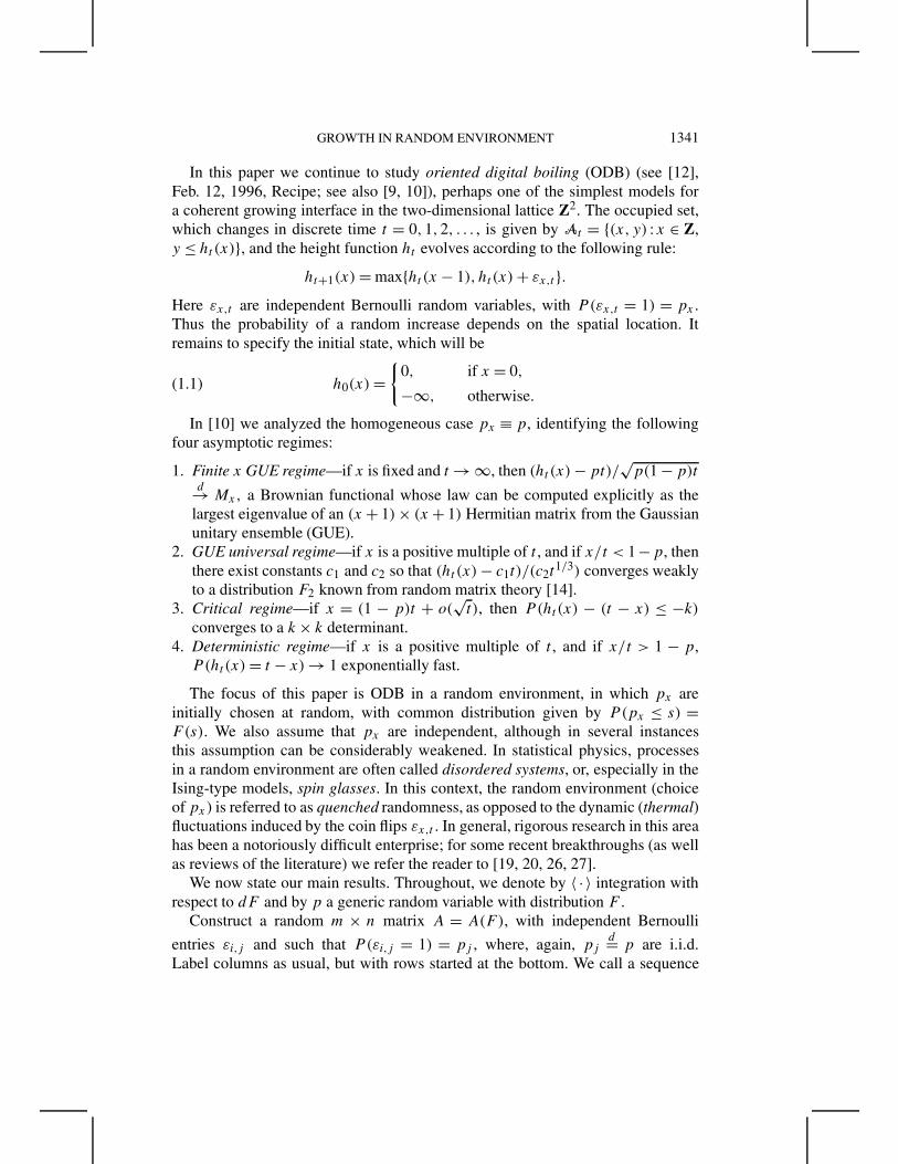
In this paper we continue to study oriented digital boiling (ODB) (see [12],Feb. 12, 1996, Recipe; see also [9, 10]), perhaps one of the simplest models fora coherent growing interface in the two-dimensional lattice Z2. The occupied set,which changes in discrete time t = 0,1,2, . . . , is given by At = {(x, y) :x " Z,y # ht (x)}, and the height function ht evolves according to the following rule:

ht+1(x) = max{ht (x ! 1), ht (x) + !x,t }.Here !x,t are independent Bernoulli random variables, with P (!x,t = 1) = px .Thus the probability of a random increase depends on the spatial location. Itremains to specify the initial state, which will be

h0(x) =!

0, if x = 0,

!$, otherwise.(1.1)

In [10] we analyzed the homogeneous case px % p, identifying the followingfour asymptotic regimes:

1. Finite x GUE regime—if x is fixed and t & $, then (ht (x) ! pt)/'

p(1 ! p)td& Mx, a Brownian functional whose law can be computed explicitly as the

largest eigenvalue of an (x + 1) ( (x + 1) Hermitian matrix from the Gaussianunitary ensemble (GUE).

2. GUE universal regime—if x is a positive multiple of t , and if x/t < 1!p, thenthere exist constants c1 and c2 so that (ht (x) ! c1t)/(c2t

1/3) converges weaklyto a distribution F2 known from random matrix theory [14].

3. Critical regime—if x = (1 ! p)t + o('

t), then P (ht(x) ! (t ! x) # !k)converges to a k ( k determinant.

4. Deterministic regime—if x is a positive multiple of t , and if x/t > 1 ! p,P (ht(x) = t ! x) & 1 exponentially fast.

The focus of this paper is ODB in a random environment, in which px areinitially chosen at random, with common distribution given by P (px # s) =F(s). We also assume that px are independent, although in several instancesthis assumption can be considerably weakened. In statistical physics, processesin a random environment are often called disordered systems, or, especially in theIsing-type models, spin glasses. In this context, the random environment (choiceof px ) is referred to as quenched randomness, as opposed to the dynamic (thermal)fluctuations induced by the coin flips !x,t . In general, rigorous research in this areahas been a notoriously difficult enterprise; for some recent breakthroughs (as wellas reviews of the literature) we refer the reader to [19, 20, 26, 27].

We now state our main results. Throughout, we denote by ) · * integration withrespect to dF and by p a generic random variable with distribution F .

Construct a random m ( n matrix A = A(F ), with independent Bernoullientries !i,j and such that P (!i,j = 1) = pj , where, again, pj

d= p are i.i.d.Label columns as usual, but with rows started at the bottom. We call a sequence

1342 J. GRAVNER, C. A. TRACY AND H. WIDOM

of 1’s in A whose positions have column index nondecreasing and row indexstrictly increasing an increasing path in A. Let H = H(m,n) be the length ofthe longest increasing path. [Sometimes, to emphasize dependence on F , we writeH = H(F) = H(m,n,F ).] The following lemma is then easy to prove [10].

LEMMA 1.1. Under a simple coupling, ht (x) = H(t ! x, x + 1).

We therefore concentrate our attention on the random matrix A from now on,switching to the height function only occasionally to interpret the results. We alsonote that Lemma 1.1 demonstrates that ODB is equivalent to the Seppäläinen–Johansson model [17, 25].

Our first theorem identifies the time constant. In the sequel, we present twocompletely different methods for proving these limits, a variational approach anda determinantal approach. The first method (which is similar to the one in [7])is based on the crucial symmetry property of H (Lemma 2.2) and provides someinformation on the longest increasing path itself; the second one is deeper and moreprecise and thus able also to determine fluctuations. Seppäläinen and Krug [26]study a related model, present yet another technique, based on an exclusion processrepresentation, and observe similar phase transitions. Throughout this paper, we let

b = b(F ) = min{s :F(s) = 1}

be the right edge of the support of dF and assume that n = "m for some0 < " < $. (Actually, n = +"m,, but we drop the integer part as it is obviouswhere it should be used and to avoid complicating expressions.) We also definethe critical values

"c ="

p

1 ! p

#!1

,

(1.2)

"-c =

"

p(1 ! p)

(b ! p)2

#!1

and define c = c(",F ) to be the time constant

c = c(",F ) = limm&$

H

m.(1.3)

Note that c determines the limiting shape of At , namely limAt /t , as t & $ forthe corner initialization given by (1.1). By virtue of the Wulff transform, it thenalso gives the speeds of some half-planes, that is, lim At /t when A0 comprisespoints below a fixed line. See [26] for much more on this issue.


THEOREM 1. The limit in (1.3) exists almost surely. If b = 1, then c(",F ) = 1for all ", while if b < 1, then

c(",F ) =

$

%

%

%

%

%

&

%

%

%

%

%

'

b + "(1 ! b)

"

p

b ! p

#

, if " # "-c,

a + "(1 ! a)

"

p

a ! p

#

, if "-c # " # "c,

1, if "c # ".Here a = a(",F ) " [b,1] is the unique solution to

"

"

p(1 ! p)

(a ! p)2

#

= 1.

Note that that )(b ! p)!2* = $ iff "-c = 0 iff there is only one critical value.

Next we turn our attention to fluctuations. In this paper we present completeresults for the pure regime "-

c < " < "c and for the (easy) deterministic regime"c < ". The composite regime " < "-

c is addressed in [11], while both criticalcases when " equals either critical value currently remain unresolved. To explainthe results, and to connect with the spin-glass terminology we have just used, weturn to a simulation. For an example, we use F(s) = 1! (1!2s)3 so that b = 1/2,"c . 6.3 and "-

c . 0.5 and run the simulation until time t = 40,000 (with a singlerealization of the environment and the coin flips). When x is close to the origin, itis clear from the picture that the interface mostly consists of sheer walls followedby flat pieces. The walls correspond to the rare sites with update probability px

close to 1/2. Those are much faster than the other sites so they pull ahead of theirleft neighbors, creating walls, and dominate their right neighbors by “feeding”them at nearly the largest possible rate. In fact, this state of affairs persists upto about x = t/3 although close to x = t/3 these effects are less pronounced. Inthe pure regime, when x/t ranges approximately from 0.333 to approximately0.863, the fluctuations are much more regular, and in fact, as we will demonstrate,asymptotically normal. For larger x/t the shape has slope !1 and no fluctuations.

For comparison, consider the case when p is uniform on [0,1/2], the casethat has "c = 1/(ln 4 ! 1) . 2.59 and "-

c = 0. The fluctuations are normal up tox/t . 0.72. Figure 1 depicts the results of simulations, first complete boundariesof two occupied sets (the top curve is the uniform case), then two details (the rightcurve is the uniform case) for x " [1000,5000].

THEOREM 2. Assume that b < 1 and "-c < " < "c. Let a be as in Theorem 1

and let

# 2 = Var(

(1 ! a)p

a ! p

)

.


FIG. 1. Two ODB simulations, as explained in the text.

Then, as m & $,

H ! cm

#'"m1/2

d& N(0,1).

Assume that p is uniform [0,1/2] to illustrate Theorems 1 and 2. Together

they imply that there exist c1 and c2 so that (ht(x) ! c1t)/(c2t)1/2 d& N(0,1),

where c1 determines the limiting shape and c2 is the variance. These two quantitiesare presented in Figure 2; c1 is the top curve and c2 is the bottom curve. Forcomparison, the shape of homogeneous ODB with px % )p* = 1/4 is also drawn(middle curve). Note that c1 and c2 approach 1/2 and 1/4, respectively, as "& 0,indicating that for small x/t the interface growth is governed by the largest updateprobability, which is close to 1/2. Finally, we do the same computation for theother example in Figure 1. The variance is now drawn only on ["-

c,1].We note that both a.s. convergence to the limiting shape [which is equivalent

to a.s. convergence in (1.3)] and its convexity follow from subadditivity, whichin turn is a consequence of the fact that this is an oriented model in whichinfluences only travel in one direction. To be more precise, fix integer sites(x1, y1), (x2, y2) " Z+ ( Z+ and define times T(x1,y1),(x2,y2) as follows. Firstwait until time T(0,0),(x1,y1) when the dynamics reaches (x1, y1). Then restart the


FIG. 2. c1 (top), c2 (bottom) and the shape for px % )p* (middle) versus x/t . The two distributionsare uniform [0,1/2] (left) and F(s) = 1 ! (1 ! 2s)3 .

dynamics from the initial state

h0(x) =!

y1, if x = x1,

!$, otherwise,

and let T(x1,y1),(x2,y2) be the time at which the occupied set reaches (x2, y2).This random variable is independent of px for x # x1 ! 1 and T(0,0),(x2,y2) #T(0,0),(x1,y1) + T(x1,y1),(x2,y2). Therefore, the subadditive ergodic theorem can beapplied as in the first chapter of [8].

The main step in the proof of Theorem 2 establishes a limit law for fluctuationsconditioned on the state of the environment. In many ways, such a result is morepertinent to understanding physical processes modeled by simple growth modelssuch as ODB.

THEOREM 3. Assume that b < 1 and "-c < " < "c. Then there exists a

sequence of random variables Gn " $ {p1, . . . , pn} and a constant g0 /= 0 (bothdepending on ") such that, as m & $,

P

(

H ! Gn

g!10 m1/3

# s*

*

*p1, . . . , pn

)

& F2(s),

almost surely, for any fixed s.

The random variables Gn = cnm are given in terms of the solution of analgebraic equation in which p1, . . . , pn appear as parameters [see (3.4) and (3.5)],while the deterministic constant g0 is specified before the statement of Lemma 3.5.The limiting distribution function F2 first arose in connection with eigenvalues ofrandom matrices ([28]; see [29] for a review). Since then it has been observedin many other contexts, including growth processes [2, 10, 16, 17, 21, 22]. Mostsuitable for computations is the identity

F2(s) = exp(

!+ $

s(x ! s)q(x)2 dx

)

,


where q is the unique solution of the Painlevé II equation

q -- = sq + 2q3,

which is asymptotic to the Airy function, q(s) 0 Ai(s) as s & $. When provinglimit laws, it is more useful that F2 can be represented as a Fredholm determinant(see, e.g., [10] and Section 3 below).

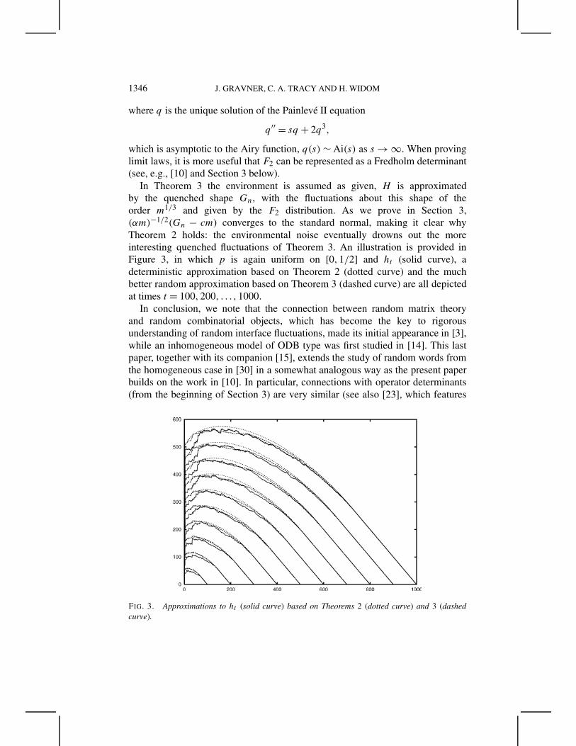
In Theorem 3 the environment is assumed as given, H is approximatedby the quenched shape Gn, with the fluctuations about this shape of theorder m1/3 and given by the F2 distribution. As we prove in Section 3,("m)!1/2(Gn ! cm) converges to the standard normal, making it clear whyTheorem 2 holds: the environmental noise eventually drowns out the moreinteresting quenched fluctuations of Theorem 3. An illustration is provided inFigure 3, in which p is again uniform on [0,1/2] and ht (solid curve), adeterministic approximation based on Theorem 2 (dotted curve) and the muchbetter random approximation based on Theorem 3 (dashed curve) are all depictedat times t = 100,200, . . . ,1000.

In conclusion, we note that the connection between random matrix theoryand random combinatorial objects, which has become the key to rigorousunderstanding of random interface fluctuations, made its initial appearance in [3],while an inhomogeneous model of ODB type was first studied in [14]. This lastpaper, together with its companion [15], extends the study of random words fromthe homogeneous case in [30] in a somewhat analogous way as the present paperbuilds on the work in [10]. In particular, connections with operator determinants(from the beginning of Section 3) are very similar (see also [23], which features

FIG. 3. Approximations to ht (solid curve) based on Theorems 2 (dotted curve) and 3 (dashedcurve).


a general inhomogeneous setup). However, randomness of the environment, whichseems to be a new feature in rigorous analysis of explicitly solvable models, thenforces our techniques to take a novel turn.

2. A variational characterization of the time constant. We start with aremark on constructing the random matrix A. The most convenient design uses asthe probability space (%,P ) a countably infinite product of unit intervals [0,1]with Lebesgue measure. A copy of the unit interval (and thus a factor in theproduct) is associated with each point in N(N and, in addition, with each positiveinteger in N. (The former factors correspond to matrix entries, and the latter to itscolumns.) If & = (mij , cj ) " % is a generic realization, we define the followingrandom variables: pj = F!1(cj ) [where F!1(x) = sup{y :F(y) < x} as usual]and !ij = 1{mij<pj }. By restricting to the m ( n rectangle at the lower right cornerof N ( N, this constructs the random matrices A for all m and n simultaneously.The following useful lemma also follows immediately.

LEMMA 2.1. If F1 # F2 are two distribution functions, the two correspondingrandom matrices A(F1) and A(F2) can be coupled so that H(F2) # H(F1).

Next we state the crucial property for the variational approach to work:conditioned on the environment, H is a symmetric function of flip probabilities.

LEMMA 2.2. A regular conditional distribution

P (H # h|p1, . . . , pn)

is a symmetric function of p1, . . . , pn.

See [10], Section 2.2, for the proof of Lemma 2.2.Somewhat loosely, we denote by Hn the random variable H obtained by fixing

p1, . . . , pn. In fact this is nothing more than a shorthand notation, for example,E('(Hn)) = E('(H) | p1, . . . , pn) for any bounded measurable function '.

The time constant c(", x) = c(", (x) for the case pj % x is given in [9]. Thenext lemma summarizes the relevant conclusions.

LEMMA 2.3. Assume that dF = (x . Then

c = c(", x) =!

2'"'

x(1 ! x) + (1 ! ")x, (1 ! x)/x > ",

1, (1 ! x)/x # ".Moreover, for every ! > 0 there exists a constant ) = ) (!) > 0 so that

P (|H/m ! c| > !) < e!)m(2.1)

for m 1 m0(!,", x).


PROOF. The formula for c follows from (3.1) of [10], while the large deviationestimate can be proved by the method of bounded differences as in Lemma 5.4of [9]. !

It turns out the following function is more convenient than c:

*(y, x) = yc(1/y, x) =!

2'

y'

x(1 ! x) + (y ! 1)x, x/(1 ! x) < y,

y, x/(1 ! x) 1 y.

Note that the partial derivative

*y(y, x) =!

y!1/2'x(1 ! x) + x, x/(1 ! x) < y,

1, x/(1 ! x) 1 y,

is decreasing in y (obviously) and increasing in x (easily checked). In particular,*(·, x) is a convex function.

We now derive a variational problem for c, initially without paying attention torigor. Start by a nice distribution function F and approximate it by the discretedistribution function given by

P

(

pj = i

k

)

=+Fk(i) = F

(

i

k

)

! F

(

i ! 1k

)

, i = 1, . . . , k.

Let , : [0,"] & [0,1], ,(0) = 0, ,(") = 1 be a nondecreasing function, with+,k(i) =,("F(i/k)) !,("F((i ! 1)/k)). Define the functionals

F (,) =+ 1

0*,

, -("F(x)), x-

" dF (x)

and

Fk(,) =k

.

i=1

*

(

+,k(i)

"+Fk(i),i

k

)

"+Fk(i).

Generate the pj ’s and denote by Ni the number of pj equal to i/k. ByLemma 2.2, we can assume flip probability 1/k in the first N1 columns, 2/kin the next N2 columns etc. Moreover, the strong law suggests that the identityNi =+Fk(i)n nearly holds. As we know the asymptotics for the longest increasingpaths in the slivers of widths Ni in which the probabilities are constant, the longestincreasing path in A is determined by the most advantageous choice of transitionpoints between the slivers. These transition points are specified by a function , asdescribed above. If we approximate the differences with derivatives, we obtain

c(",F ) = limk&$

c(",Fk)

= limk&$

max,

k.

i=1

c

(

"+Fk(i)

+,k(i),i

k

)

+,k(i)


= limk&$

max,

Fk(,)

= limk&$

max,

k.

i=1

*

(

, -(

"F

(

i

k

))

,i

k

)

"F -(

i

k

)

1k

= max,

F (,).

At this point, we remark that a connection between longest increasing pathsand variational problems has appeared before in the literature. The result closestto ours is by Deuschel and Zeitouni [7], who used a variational approach tostudy a variant of Ulam’s problem. In their case, a number of points in the unitsquare is chosen independently according to some distribution with a density,then a longest sequence, increasing in both coordinates, is extracted from thissample. The Deuschel–Zeitouni functional is different from ours as the length ofthe longest increasing path has a nontrivial dependence on " (i.e., through c) inour case.

The (integrated) Euler functional for the variational problem is

*y,

, -(x),F!1(x/")- = a

or, writing g(x) =, -("F(x)),

*y(g(x), x) = a.(2.2)

Since *y # 1 and equal to 1 if and only if x/(1 ! x) 1 y, the integration constanta " [0,1]. If a = 1, then g(x) # x/(1 ! x), *(g(x), x) = g(x) and

c(",F ) =+ 1

0, -("F(x))" dF (x) = 1.

Assume now that b < 1. In this case, it is necessary to specify g only on [0, b).However, (2.2) gives

g(x) = x(1 ! x)

(a ! x)2 .(2.3)

The constant a is given by the boundary conditions. Assuming that (2.3) holds on[0, b],

1 = "+ b

0g(x) dF (x) = "

+ b

0

x(1 ! x)

(a ! x)2 dF (x).(2.4)

The smallest the last integral can be is when a = 1, which yields the condition

1 > "

+ b

0

x

1 ! xdF (x) = "

"c.


On the other hand, the largest that the integral in (2.4) can be is when a = b.Therefore, if " " ("-

c,"c), we have found the minimizer and

c(",F ) =+ b

0*(g(x), x)" dF (x) = "

"!p2 ! a2p + 2ap

(a ! p)2

#

,

which reduces, upon using the defining equation for a, to the formula inTheorem 1.

If " < "-c, the minimizer, has to make a jump of size 1!"/"-

c at ". The naturalinterpretation for this is that the minimizer given by (2.3) is used in the lower leftpart of A with dimensions ("/"-

c)m ( (n ! 1). To the resulting increasing path inthis submatrix one needs to add the number of 1’s in the upper segment of length(1 ! "/"-

c)m in the last column, in which nearly the largest probability b is used.Therefore,

c(",F ) = c("-c,F )

"

"-c

+ b

(

1 ! "

"-c

)

,

which again reduces to the appropriate formula in Theorem 1.We now proceed to give a proof Theorem 1, the heart of which is a somewhat

involved multistage approximation scheme.

PROOF OF THEOREM 1 WHEN b = 1. This follows simply by observing that,for any ! > 0, maxj pj & b a.s. as m & $. Since a trivial lower bound is obtainedby using only the column with the largest pj , one concludes that lim inf H/m 1 ba.s. !

PROOF OF THEOREM 1 WHEN " " ("-c,"c). We begin with the following

lemma.

LEMMA 2.4. Assume that a sequence of distribution functions FN convergesto F in the usual sense (i.e., the induced measures converge weakly). Assume alsothat b(FN) & b(F ) and that "N & ". Then c("N,FN) & c(",F ) (as given inTheorem 1).

PROOF. If a- > b(F ) and

"

+

x(1 ! x)(a- ! x)!2 dF (x) > 1,

then, for a large N , a- > b(FN) and, since the integrand is bounded,

"N

+

x(1 ! x)(a- ! x)!2 dFN(x) > 1.

Hence aN = a("N,FN) > a-. If aN & a0, then x(1 ! x)(aN ! x)!2 converges tox(1 ! x)(a0 ! x)!2 uniformly for x " [0, a-] and so

1 = "N

+

x(1 ! x)(aN ! x)!2 dFN(x) & "

+

x(1 ! x)(a0 ! x)!2 dF (x).


Therefore a0 = a(",F ) and consequently aN & a(",F ). As x(aN ! x)!1 alsoconverges uniformly on [0, a-],

c("N,FN) = aN + "N(1 ! aN)

+

x(aN ! x)!1 dFN

& a + "(1 ! a)

+

x(a ! x)!1 dF = c(",F ). !

First we assume that F is nice, that is, a one-to-one function on [-, b] 2 (0,1),with F(-) = 0 and F(b) = 1, and continuously differentiable on (0,1). We alsoassume that . is the class of nondecreasing convex functions , " C2[0,"], with,(0) = 0, ,(") = 1, , -(0) 1 -/2. This last assumption is necessary because*(y, x) is not Lipshitz near y = 0.

LEMMA 2.5. Assume that " " ("-c,"c). Among all , " . , the functional

F (,) is uniquely maximized by

,(x) =+ x

0g,

F!1(u/")-2

du,

where g is given by (2.3).

PROOF. This follows from standard calculus of variations. Both , -(0) 1 -/2and convexity of , are easily checked. !

We now justify the approximation steps in the heuristic argument, using thesame notation. First, if ! > 0 is fixed, then with probability exponentially (in n)close to 1,

(1 ! !)+Fk(i)n # Ni # (1 + !)+Fk(i)n

for every i = 1, . . . , k. By obvious monotonicity, the longest increasing pathin A is then bounded above by the longest increasing path in A- in which allNi = (1 + !)+Fk(i)n, and therefore we can get an upper bound by increasing "to "(1 + 2!) and assuming Ni = +Fk(i)n. A lower bound is obtained similarly.As our final characterization of c is continuous with respect to " (Lemma 2.4), wecan, and will, assume that Ni =+Fk(i)n from now on.

The above paragraph eliminates randomness of pj ’s; we now proceed to replacethe coin flips with deterministic quantities. Again, fix an ! > 0 and let M = !m.For j1 # j2 and i = 1, . . . , n, consider the longest increasing paths /j1,j2,i between(Fk(i!1)n, j1) (noninclusive) and (Fk(i)n, j2) (inclusive). Then, with probabilityexponentially close to 1, the length of any /j1,j2,i is at most

(1 + !)c(

+Fk(i)n

M3(j2 ! j1)/M4 ,i

k

)

M3(j2 ! j1)/M4

= (1 + !)*(

M3(j2 ! j1)/M4+Fk(i)n

)

+Fk(i)n.


(This uses Lemma 2.3 when j2 ! j1 is divisible by M and fills the rest bymonotonicity. Note that Lemma 2.3 is therefore only applied finitely many timesfor fixed ! and k.) The lower bound is obtained by rounding down instead of up. Itfollows that the length of any /j1,j2,i is bounded above (resp. below) by

*

(

j2 ! j1

+Fk(i)n

)

+Fk(i)n(2.5)

computed on the matrix of size (m + M)( n [resp. (m!M)( n]. Once again wecan use continuity to assume that the length of any /j1,j2,i is given by (2.5).

It remains to show that the discrete deterministic optimization problemmax, Fk(,) is for large k close to its continuous counterpart max, F (,). Tothis end, we first prove that we can indeed restrict the set of function , tothose in . , that is, those that are convex and have a large enough derivative.Let +x1 = "+Fk(i), +x2 = "+Fk(i + 1), +y1 = +,k(i), +y2 = +,k(i + 1),+y =+y1 ++y2, p1 = i/n, p2 = (i + 1)/n. Then

*

(

+y1

+x1,p1

)

+x1 + *(

+y !+y1

+x2,p2

)

+x2(2.6)

is nondecreasing with decreasing +y1 as soon as p1 # p2 and +y1/+x1 1+y2/+x2. This means that the maximum is achieved at a convex , . Similarly, theexpression (2.6) is nondecreasing with increasing +y1 if p1 1 - and +y1/+x1 <(/(1 ! (), and therefore the maximum is achieved at a , ". .

Next we note that

Fk(,) #k

.

i=1

*,

, -("F(i/k)), i/k-

"+Fk(i),

while

F (,) 1k

.

i=1

*,

, -("F(i/k)), i/k-

"+Fk+1(i).

Therefore, max, Fk(,) # max, F (,) + O(1/k). As a lower bound is obtainedsimilarly, this concludes the proof for nice distribution functions F .

To prove the general case, we again use Lemmas 2.1 and 2.4. For an arbitrarydistribution function, choose nice F±

N so that F!N # F and F · 1(1/N,1] # F+

N

and F±N & F and b(F±

N ) & b(F ). Then c(",F±N ) & c(",F ). By Lemma 2.1,

it immediately follows that lim supH/m # c(",F ) a.s.The lower bound, however, does not immediately follow as F is not below F+

N .The remedy for this is to assume that F(1/N) < 1/2, replace " with "- < " andobserve that the distribution F will induce, with probability exponentially closeto 1, at least (" ! "-)m/4 probabilities pj 1 1/N . Therefore the length of thelongest increasing path in an m("m matrix using F is eventually above the length


of the longest increasing path in an m ( "-m matrix using F+N . By Lemma 2.4,

lim inf H/m 1 c(",F ) a.s. !

PROOF OF THEOREM 1 WHEN " # "-c . Applying the same strategy as before

we construct sequences {F±N } of distribution functions which satisfy F!

N # F #F+

N and for which Theorem 1 already holds, and such that c(F!N ) and c(F+

N )approach the same limit as N & $. Lemma 2.1 will then complete the proof.(We suppress " from the notation, since it is the same throughout this proof.)

Take a sequence 0N 5 0 such that b ! 0N are points of continuity of F . LetF±

N agree with F outside [b ! 0N,b), while on [b ! 0N,b) the two functionsare constant: F!

N % F(b ! 0N) and F+N % 1. Let !N = 1 ! F(b ! 0N); note that

!N & 0 and dF!N = 1(0, b!0N) dF + !N (b and dF+

N = 1(0, b!0N) dF + !N (b!0N .Clearly the already proved part of Theorem 1 applies to both F+

N and F!N .

We proceed to show that a(F!N ) & b. If this does not hold, the fact that

a(F!N ) > b(F!

N ) = b implies that there exists an 0 > 0 so that a(F!N ) 1 b + 0

along a subsequence. Then ( = )p(1 ! p)[(b ! p)!2 ! (b + 0! p)!2]* > 0 and

1 = "+ b!0N

0

x(1 ! x)

(a(F!N ) ! x)2

dF + "!Nb(1 ! b)

(a(F!N ) ! b)2

# "+ b

0

x(1 ! x)

(b + 0! x)2 dF + "!Nb(1 ! b)

02(2.7)

# !( + "

"-c

+ "!Nb(1 ! b)

02 ,

along the same subsequence. As N & $, this yields a contradiction with " # "-c.

Nowc(F!

N ) = a(F!N ) + " ,

1 ! a(F!N )

-

((+ b!0N

0

x

a(F!N ) ! x

dF + !Nb

a(F!N ) ! b

)

.(2.8)

By (2.7),

!Nb

a(F!N ) ! b

# a(F!N ) ! b

"(1 ! b)& 0.

To show that/

1{p#b!0N }p/,

a(F!N ) ! p

-0 & )p/(b ! p)*(2.9)

we note that the integrand on the left-hand side of (2.9) is uniformly integrable[as it is bounded by p/(b ! p), which is square-integrable] and converges to theintegrand on the right-hand side a.s. By (2.8) and (2.9),

c(F!N ) & b + "(1 ! b))p/(1 ! p)*.

The argument for c(F+N ) is very similar and hence omitted. !


PROOF OF THEOREM 1 WHEN " 1 "c . If " 6 "c, then a(",F ) 6 1 andhence c(",F ) 6 1. !

We note that the above proof of Theorem 1 actually shows exponentialconvergence to c, that is, (2.1) in Lemma 2.3 holds in a random environment aswell. Also, once probabilities are ordered using Lemma 2.1, one could investigateconvergence, in the sense of [7] and [24], of the longest increasing path in A tothe maximizer of F (,). This is easy to prove if F is nice (cf. Lemma 2.5), but itactually holds whenever the maximizer is unique.

We conclude this section by showing that the deterministic case indeed has nofluctuations.

PROPOSITION 2.6. Assume that b < 1 and " > "c. Then P (H = m)converges to 1 exponentially fast [and therefore P (H = m eventually) = 1].

PROOF. We begin by modifying the construction from Section 3.3.1 of [9].Recall that a random m ( n matrix is the lower left corner of an infinite randommatrix. For an (i, j) " N ( N, let 0(i,j ) = inf{k 1 1 : !(i+k,j) = 0} be the relativeposition of the first 0 above (i, j) and let 1(i,j ) = inf{k 1 1 : !(i,j+k) = 1} be therelative position of the first 1 to the right of (i, j).

Now define i.i.d. two-dimensional random vectors X1 = (11,01), X2 =(12,02), . . . as follows:

11 = 1(0,1), 01 = 0(11,1),

12 = 1(11,1+01), 02 = 0(11+12,1+01),

13 = 1(11+12,1+01+02), 02 = 0(11+12+13,1+01+02),

· · · .Let Sk = (0,1) + X1 + · · · + Xk be the corresponding random walk, and let Tm

(resp. T -n) be the first time Sk is in {(x, y) :x > n} [resp. {(x, y) :y > m}]. If

T -m < Tn, then there is an increasing path of 1’s inside the m ( n rectangle which

goes through its “roof” without skipping a row; thus

{H < m} 2 {Tn # T -m}.

Therefore, we need to show that P (Tn # T -m) goes to 0 exponentially fast. To this

end, note that, for any ! > 0,

P (Tn # T -m) # P (Tn 7 T -

m # !m)

+$.

k=!mP

,

11 + · · · + 1k 1 "(01 + · · · + 0k)-

.(2.10)

If we show that 11 and 01 have exponential tails, and that E(11) ! "E(01) < 0,then we can choose a small enough ! > 0 so that the upper bound in (2.10) decays


exponentially. First, P (11 1 k) = )1!p*k!1 and so E(11) = 1/)p*. Moreover, theconditional distribution of p given that a single coin flip gives 1 is

dF1(x) = 1)p*x dF (x);

therefore

P (01 1 k) =+ 1

0xk!1 dF1(x) = )pk*

)p* ,

and so E(01) = )p/(1 ! p)*/)p*. !

3. The saddle-point method and fluctuations. Throughout this section, weassume that b < 1 and that " = n/m is fixed (but see Remark 3 at the end). Inaddition, our standing assumption is that

"-c < " < "c.

We investigate the limiting behavior of P (H # h) without using results provedin Section 2. An asymptotic analysis of this quantity when " < "-

c is carried outin [11].

We begin with deterministic inhomogeneous ODB, in which the j th columnis assigned a fixed deterministic probability pj . At first, our derivation will usea fixed n and no particular properties of the eventual random choice of theenvironment. For notational convenience, we therefore drop the subscript n, whichpractically every quantity would otherwise have. See the discussion preceding thekey formula (3.6), where the random environment is reintroduced.

As explained in [10, Section 2.2], we have

P (H # h) =1

(1 ! pj )m Dh('),

where Dh is the h ( h Toeplitz determinant with symbol

(1 ! z!1)!mn

1

j=1

(1 + rj z)

and rj = pj/(1 ! pj ). Applying an identity of Borodin and Okounkov [6] (seealso [4]) this becomes

P (H # h) = det(I ! Kh),

where Kh is the infinite matrix acting on 22(Z+) with j, k entry

Kh(j, k) =$.

2=0

('!/'+)h+j+2+1('+/'!)!h!k!2!1.


The subscripts here denote Fourier coefficients and the functions '± are theWiener–Hopf factors of ', so

'+(z) =n

1

j=1

(1 + rj z), '!(z) = (1 ! z!1)!m.

The matrix Kh is the product of two matrices, with j, k entries given by(

'+'!

)

!h!j!k!1= 1

2/ i

+

1

(1 + rj z) (z ! 1)m z!m+h+j+k dz

and(

'!'+

)

h+j+k+1= 1

2/ i

+

1

(1 + rj z)!1(z ! 1)!m zm!h!j!k!2 dz.

The contours for both integrals go around the origin once counterclockwise; in thesecond integral 1 is on the inside and all the !r!1

j are on the outside.

Eventually we let m, n & $ and take h = cm + sm1/3, where c, as yet to bedetermined, gives the transition between the limiting probability being 0 and thelimiting probability being 1. In [10] we considered the case where all the pj werethe same. We found that with c chosen as in Lemma 2.3 we could do a steepestdescent analysis. The conclusion was that the product of the two matrices scaled,by means of the scaling j & m1/3x, k & m1/3y, to the square of the integraloperator on (0,$) with kernel Ai(gs + x + y), where g is another explicitlydetermined constant. This gave the limiting result

limn&$ P (H # cm + sm1/3) = F2(gs),

where F2(s) is the Fredholm determinant of the Airy kernel on (s, $). We can dovery much the same here. If h = cm + sm1/3 and we set

,(z) =1

(1 + rj z) (z ! 1)m z!(1!c)m,

then(

'+'!

)

!h!j!k!1= 1

2/ i

+

,(z) zsm1/3+j+k dz,(3.1)

(

'!'+

)

h+j+k+1= 1

2/ i

+

,(z)!1 z!sm1/3!j!k!2 dz.(3.2)

To do an eventual steepest descent we define

$ (z) = 1m

log,(z) = "

n

n.

j=1

log(1 + rj z) + log(z ! 1) + (c ! 1) log z,


and look for zeros of

$ -(z) = "

n

n.

j=1

rj

1 + rj z+ 1

z ! 1+ c ! 1

z.(3.3)

The number of zeros equals 1 plus the number of distinct rj . There is a zerobetween two consecutive 1/rj and, in general, two other zeros which are eitherunequal reals or a pair of complex conjugates. In the exceptional case there is asingle real zero of multiplicity 2. We choose c so that we are in this exceptionalcase. If the double zero is at z = u, then u and c must satisfy the pair of equations

"

n

n.

j=1

rj

1 + rju+ 1

u ! 1+ c ! 1

u= 0,

"

n

n.

j=1

(

rj

1 + rju

)2

+ 1(u ! 1)2 + c ! 1

u2 = 0.

If we multiply the second equation by u and subtract, we get

"

n

n.

j=1

rj

(1 + rju)2 = 1(u ! 1)2 .(3.4)

The first equation gives

c = 11 ! u

! "n

n.

j=1

rju

1 + rju.(3.5)

Conversely, if the second pair of equations is satisfied, then so is the first.

LEMMA 3.1. Assume that "n!1 2

rj < 1 and set u = max{!1/rj }. Then(3.4) has a unique solution u " (u, 0) and if c is then defined by (3.5), we havec " (0, 1).

PROOF. The left-hand side of (3.4) decreases from $ to "n!1 2

rj as u runsover the interval (u, 0) whereas the right-hand side increases and has the value 1at u = 0. Our assumption implies the first statement of the lemma. As for thesecond, c > 0 since u < 0 and each 1 + rju > 0. Moreover, Schwarz’s inequality,our assumption and (3.4) give

"

n

. rj

1 + rju#

3

"

n

.

rj

41/2 3

"

n

. rj

(1 + rju)2

41/2

<1

1 ! u.

Hence

c <1

1 ! u! u

1 ! u= 1. !


To derive the asymptotics using steepest descent we have to compute $ ---(u)and understand the steepest descent curves. For the first we multiply (3.3) by z,differentiate twice and use the fact that $ -(u) = $ --(u) = 0 to obtain

u$ ---(u) = !2"n

n.

j=1

r2j

(1 + rju)3 + 2(u ! 1)3 .

Note that $ ---(u) > 0 since u < 0.There are three curves emanating from z = u on each of which 8$ is constant.

One is 8 z = 0, which is of no interest. The other two come into u at angles ±//3and ±2//3. Call the former C+ and the latter C!. Approximate shapes of thesecurves are illustrated in Figure 4. For the integral involving ,(z) we want |,(z)| tohave a maximum at the point u on the curve and for the integral involving ,(z)!1

we want |,(z)| to have a minimum at u. Since $ ---(u) > 0 the curve for ,(z) mustbe C+ and the curve for ,(z)!1 must be C!.

As for the global natures of the curves, C± can only end at a zero of ,(z)±1,at a zero of $ -(z) or at infinity. The two curves are simple and cannot intersectsince |,(z)| is decreasing on C+ as we move away from z = u while |,(z)| isincreasing on C!. It follows that C+ closes at z = 1, while the two branches ofC! go to infinity. From the fact that

8$ (z) = "

n

n.

j=1

arg(1 + rj z) + arg(z ! 1) + (c ! 1) arg z

is constant on C! we can see that the two branches go to infinity in the directionsarg z = ±c//(c + "(1 ! 3)), where 3 is the fraction of rj equal to zero (whichis the same as the fraction of the pj equal to zero). Observe that in the integral

FIG. 4. The steepest descent curves C± as described in the text.


in (3.1) the path can be deformed into C+ and in the integral in (3.2) the path canbe deformed into C!. Both contours will be described downward near u.

To see formally what steepest descent gives, we replace our matrices M(j, k)

depending on the parameter m and acting on 22(Z+) by kernels m1/3M(m1/3x,

m1/3y) acting on L2(0, $). Thus (3.1) becomes the operator with kernel

12/ i

m1/3+

em$ (z) zm1/3(s+x+y) dz.

If steepest descent worked, the main contribution would come from theimmediate neighborhood of z = u. We would set z = u+* , make the replacements

$ (z) & $ (u) + 16$

---(u)* 3 and z & ue*/u

in the integral and integrate (downward) on the rays arg * = ±//3. The aboveintegral becomes

em$ (u) um1/3(s+x+y) 12/ i

m1/3+

e(m/6)$ ---(u)* 3+m1/3(s+x+y)*/u d*,

and we can then replace the rays by the imaginary axis (downward). The variablechange * & !i*/m1/3 replaces this by (recall that the Airy function is defined byAi(x) = 1

2/5 $!$ ei* 3/3+ix* d* )

!em$ (u) um1/3x 12/

+ $

!$e(i/6)$ ---(u)* 3!i(s+x+y)*/u d*

= !em$ (u) um1/3(s+x+y) |u|g Ai(g(s + x + y)),

where we have set

g = |u|!1612$

---(u)7!1/3

.

Thus, if we multiply the matrix entries on the left-hand side of (3.1) by

!e!m$ (u) u!m1/3s!j!k,

then the result has as scaling limit the operator on L2(0, $) with kernel

|u|g Ai(g(s + x + y)).

Similarly if we multiply the matrix entries on the left-hand side of (3.2) by

!em$ (u) um1/3s+j+k,

then the result has as scaling limit the operator on L2(0, $) with kernel

|u|!1g Ai(g(s + x + y)).


It follows that the product of the two matrices has in the limit the same Fredholmdeterminant as the operator with kernel

g2+ $

0Ai(g(s + x + z))Ai(g(s + z + y)) dz

= g

+ $

0Ai(g(s + x) + z)Ai(g(s + y)) dz,

which in turn has the same Fredholm determinant as the kernel+ $

0Ai(gs + x + z)Ai(gs + z + y) dz.

This Fredholm determinant equals F2(gs).Assuming the argument we sketched above goes through we will have shown

that, in some sense,

limn&$ P (H # cm + sm1/3) = F2(gs),

where c and g are as above and are determined once we know the pj and ".We begin the rigorous justification by introducing some notation. Recall that

we consider a random environment in which the probabilities pj are chosenindependently with distribution function F . We explained the notation Hn afterLemma 2.2; in addition, we give the subscript n to the quantities $n(z), un, gn andcurves C±

n to emphasize that they are functions of p1, . . . , pn. Therefore

P (H # h) = )P (Hn # h)*,where ) · * is the expected value with respect to p1, . . . , pn.

Our object is to show that with probability 1, for each fixed s,

P (Hn # cn m + sm1/3) = F2(gn s) + o(1)(3.6)

as n & $. We will demonstrate these asymptotics by pointing out the necessarymodifications to the argument in [10].

All the !1/rj in our previous discussion are contained in the interval (!$, 1 ],where 1 = 1 ! 1/b. (Recall that b is the maximum of the support of dF .) Let Fn

be the empirical distribution function given by

dFn = n!1.

(pj

and let ) · *Fn denote the integration with respect to dFn. Recall the Glivenko–Cantelli theorem, which says that, with probability 1, Fn converges uniformly to Fas n & $.

We first show that, under our standing assumptions, the quantities cn and un

of Lemma 3.1 converge almost surely as n & $ to the corresponding quantitiesassociated with the distribution function F . Recall that we set r = p/(1!p), p =r/(1+ r). We remark that c0 in the following lemma is the same as c in Theorem 1,and u0 = (a !1)/a. The notation has changed to conform to (3.4) and (3.5), whichare in turn chosen to connect with the saddle-point approach in [10].


LEMMA 3.2. The equation

"

"

r

(1 + ru0)2

#

= 1(u0 ! 1)2

has a unique solution u0 " (1, 0) and if c0 is then defined by

c0 = 11 ! u0

! ""

ru0

1 + ru0

#

,

we have c0 " (0, 1).

PROOF. The argument goes almost exactly as for Lemma 3.1. The assumption" < "c is equivalent to ")r/(1 + ru)2* > 1/(u ! 1)2 when u = 1 , while " > "-

c

yields the opposite inequality when u = 0. !

Note that one obtains un as u0, except that the expectation ) · * is replaced bythe expectation ) · *Fn .

LEMMA 3.3. Almost surely, un & u0 and cn & c0 as n & $.

PROOF. Integration by parts gives"

r

(1 + rz)2

#

=+ b/(1!b)

0(1 ! F(p))

d

dr

r

(1 + rz)2 dr.

The derivative in the integrand is uniformly bounded for z in any compact subsetof the complement of (!$, 1 ]. Hence the expected value is continuous in F anddifferentiable for z /" (!$, 1 ]. Moreover,

4

4z

(

"

"

r

(1 + rz)2

#

! 1(z ! 1)2

)

is negative, hence nonzero, at z = u0. The statement concerning un thereforefollows from the fact that Fn & F uniformly and the implicit function theorem.The assertion for cn then follows by a similar integration by parts. !

LEMMA 3.4. There exists a (deterministic) wedge W with vertex v > 1 ,bisected by the real axis to the left of v, such that, almost surely, the curves C±

n lieoutside W for sufficiently large n.

PROOF. First we show that, if ! is small enough, C!n is disjoint from the disc

D(1, !) = {z : |z ! 1 | # !}.From the facts that $ -

n(un) = $ --n (un) = 0, $ ---

n (un) > 0 and $ -n(z) /= 0 for z "

(1, un), it follows that $n is strictly increasing in the interval (1, un). Therefore,


FIG. 5. Wedge W , angle !1 and disk D(1, !) as described in the proof of Lemma 3.4.

we can choose small enough ! > 0 and ( > 0 so that $n(1 + !) < $n(un) ! 2( forall sufficiently large n. In addition, if ! is small enough,

log |z ! 1| + (cn ! 1) log |z| < log |1 + !! 1| + (cn ! 1) log |1 + !| + (for all z " D(1, !). Now each |1+rj z|, and so its logarithm, achieves its maximumon D(1, !) at the point z = 1 + !. By combining the last three observations, wesee that everywhere on D(1, !) we have

9$n(z) < $n(1 + !) + ( < $n(un) ! (.Since 9$ achieves its minimum on C!

n at z = un, the curve must be disjoint fromD(1, !).

For a small !1 > 0 (possibly much smaller than !), denote by W - the wedgewith vertex 1 ! !/2 bounded by the real axis to the left of 1 ! !/2 and the rayarg(z ! 1 + !/2) = / ! !1. Our next step is to show that C!

n is disjoint from W -

if !1 is small enough. As 8$n(z) is constant on the portion of C!n in the upper

half-plane,

"

n

n.

j=1

arg(1 + rj z) + arg(z ! 1) + (cn ! 1) arg z = cn/,

where all arguments lie in [0, / ]. For z " W -,

arg(z ! 1) + (cn ! 1) arg z 1 cn arg z 1 cn(/ ! !1).

Since b is in the support of dF , the strong law implies that, almost surely, at leasta positive fraction 0 of the !1/rj lie in the interval [1 ! !/2, 1 ] for sufficientlylarge n. The contribution of these terms (and nonnegativity of the others) in thefollowing sum provides a lower bound valid for z " W -:

"

n

n.

j=1

arg(1 + rj z) 1 "0(/ ! !1).

Hence, for z " W -,

8$n(z) 1 "0(/ ! !1) + cn(/ ! !1) = ("0+ cn) (/ ! !1) > cn/,


if !1 is chosen to be small enough. Therefore, C!n is disjoint from the wedge W - for

sufficiently small !1. By symmetry, C!n is disjoint from the reflection of W - over

the imaginary axis. We have shown that the curve is also disjoint from D(1, !) andthe union of the disc and the two wedges contains a wedge of the form describedin the statement of the lemma.

This establishes the statement of the lemma concerning C!n . Since C+

n is to the“right” of C!

n (it begins to the right and they cannot cross), the statement for C+n

follows automatically. !

In the following lemma $0 denotes the function $ associated with thedistribution F ,

$0(z) = ")log(1 + rz)* + log(z ! 1) + (c0 ! 1) log z

and

g0 = |u0|!1612$

---0 (u0)

7!1/3.

LEMMA 3.5. Almost surely, z$ -n(z) & z$ -

0(z) uniformly outside the wedge Wof Lemma 3.4.

PROOF. We have

z$ -n(z) ! z$ -

0(z) = "+

rz

1 + rzd(Fn(p) ! F(p)) + cn ! c0

= "+ b/(1!b)

0(Fn(p) ! F(p))

z

(1 + rz)2 dr + cn ! c0.

The last term goes to 0 by Lemma 3.3. The last factor in the integrand is uniformlybounded for r " (0, b/(1 ! b)), z /" W and z bounded. Thus z$ -

n(z) & z$ -0(z)

uniformly on bounded subsets of the complement of W . If z is sufficiently largeand outside W , then it is outside some wedge with vertex 0 bisected by the negativereal axis, and on the complement of any such wedge

+ b/(1!b)

0

|z||1 + rz|2 dr

is uniformly bounded. Thus z$ -n(z) & z$ -

0(z) uniformly throughout the comple-ment of W . !

The preceding lemmas show that the curves C±n are uniformly smooth, as we

now argue. The function $ -0(z) can have no other zero in the complement of

(!$, 1) than at z = u0. This follows from uniform convergence and the factthat the corresponding statement holds for the $n(z). Thus the functions $ -

n(z) areuniformly bounded away from zero on compact subsets not containing u0. As wemove outward (i.e., away from un) along C±

n , 8$ is constant and 9$ is increasing


on C!n and decreasing on C+

n . It follows that if s measures arc length on the curves,then, for z " C±

n ,

dz

ds= : |$ -

n(z)|$ -

n(z).(3.7)

This shows that the C±n are uniformly smooth on compact sets (to be more

precise, the portions in the upper and lower half-planes are). Moreover, theyare uniformly close on compact sets to the corresponding curves C±

0 for thedistribution function F . In particular, the length of C+

n is O(1).To see what happens for large z on C!

n observe that

limz&$ z$ -

n(z) = "+ cn > 0

uniformly in n. This and (3.7) show that |z| is increasing as we move far enoughout along C!

n . If 5 is an arc of C!n going from a to b, then

+

5|$ -

n(z)|ds =+

5$ -

n(z) dz = $n(b) ! $n(a).

Hence the length of 5 is at most |b ! a| times

maxz"[a,b] |$ -n(z)|

minz"5 |$ -n(z)|

,

where [a, b] is the line segment joining a and b, as long as this segment does notmeet (!$, 1). It follows from the above, for example, that the L1 norm of thefunction (1 + |z|2)!1 on C!

n is O(1).In [10] we needed asymptotics with error bounds for all j, k # h and this

required a more careful analysis of the integrals in (3.1) and (3.2) than weindicated; instead of the steepest descent curves passing through the same pointthey pass through different, but nearby, points. With what we now know we canshow that these curves are uniformly smooth with uniformly regular behavior nearinfinity, and this is what is needed to see that in our case the asymptotics holduniformly in n.

LEMMA 3.6. Almost surely, gn & g0 /= 0 and (3.6) holds.

PROOF. The first statement follows from Lemmas 3.3 and 3.5 and the factthat the $ -

n(z) have only two zeros outside (!$, 1 ] counting multiplicity, andtherefore $ ---(u0) /= 0.

To establish (3.6), one now has to go through the steepest descent argumentin [10], Section 3.1.2, and make some obvious changes, justified by the results ofthis section. For the analogue of Lemma 3.1 there, for example, we would add thephrase “and all sufficiently large n” to the end of the statement. At the end of thesecond sentence of the proof we would add the phrase “since $ ---

n (un) is uniformly


bounded away from zero the length of C+n is O(1).” After the last sentence we

would add “again since the length of C+n is O(1).” Analogous changes need to be

made throughout the argument and we skip further details. !

PROOF OF THEOREM 3. By Lemma 3.6, we can take Gn = cnm. !

PROOF OF THEOREM 2. Note first that

# 2 = Var(

ru0

1 + ru0

)

,

where u0 is as in Lemma 3.2 (and, as we remarked earlier, c0 = c).The proof rests on the crucial property (3.6) and the fact that n1/2(Fn ! F)

converges in distribution to a Brownian bridge B with an appropriate covariancestructure; in particular B is a Gaussian random element in D[0,1] ([5], Theo-rem 14.3). By the Skorohod representation theorem, we can couple Fn and B onsome probability space %0 so that

n1/2(Fn ! F) & B(3.8)

in fact converges for every & "%0 ([5], Theorem 6.7). We now prove that, underthis coupling, the solution un of (3.4) satisfies

un = u0 + n!1/2 U + o(n!1/2),(3.9)

for every & and for some Gaussian random variable U .To establish (3.9), define

6n(u) = ""

r

(1 + ru)2

#

Fn

! 1(u ! 1)2 ,

60(u) = ""

r

(1 + ru)2

#

! 1(u ! 1)2 .

By Lemma 3.6 and its proof, there exists a (deterministic) neighborhood U 2 Cof u0 in which, with probability 1, un (resp. u0) is for large n the unique solutionto 6n(u) = 0 [resp. 60(u) = 0]. Therefore we can choose a fixed contour C in Usuch that un and u0 are given by

un = 12/ i

+

C

6 -n(u)

6n(u)udu, u0 = 1

2/ i

+

C

6 -0(u)

60(u)udu.

By (3.8), we have, uniformly for u " C,

6n(u) = 60(u) + n!1/2"

"

r

(1 + ru)2

#

B+ o(n!1/2).

Here ) · *B is the expectation with respect to dB , but by integration by parts (as inthe proof of Lemma 3.3) we can make B appear in the integrand. Therefore

6 -n(u)

6n(u)= 6 -0(u)

60(u)+ n!1/2"

d

du

)r/(1 + ru)2*B60(u)

+ o(n!1/2).


If we multiply this identity by u/2/ i and integrate over C the left-hand sidebecomes un; the first term on the right-hand side becomes u0 while the secondterm becomes n!1/2 U , where

U = !" )r/(1 + ru0)2*B

6 -0(u0)

is a Gaussian random variable. This proves (3.9).Let

'n(u) = 11 ! u

! ""

r

1 + ru

#

Fn

,

so that cn = 'n(un). We claim that

cn = 'n(u0) + O(n!1).(3.10)

To see this, we use the fact that '-n(un) = 0 to write

cn = 'n(un) = 'n(u0) + (un ! u0)2+ 1

0t'--

n

,

tun + (1 ! t)u0-

dt.

Thus, (3.10) follows from (3.9) and the uniform boundedness of the 7--n(u) near

u = u0.Now, by the central limit theorem,

'n

8

1n

n.

j=1

rju0

1 + rju0!

"

ru0

1 + ru0

#

9

converges in distribution to a Gaussian random variable X with mean 0 andvariance # 2. Therefore,

'n(cn ! c0)

d& "X.(3.11)

Finally, (3.6) implies that, for any ( > 0,

P (!(m1/2 # H ! cnm # (m1/2) & 1.(3.12)

[In fact, (3.6) implies that the above statement holds with probability 1 before theexpectation with respect to p1, . . . , pn is taken, that is, if H is replaced by Hn.] Itfollows from (3.11) and (3.12) that

(H ! c0 m)/'

md& '

"X,

which concludes the proof. !

REMARK 1. We did not need the full force of (3.6) for the above proof to gothrough. Instead, a much weaker property (3.12) suffices.


REMARK 2. As mentioned in the Introduction, independence of pn is notnecessary for the results of this section to hold. Indeed, one only needs theGlivenko–Cantelli theorem for convergence in probability of H/m to the timeconstant; hence ergodicity of p1,p2, . . . is enough. Furthermore, a strong enoughmixing property of this sequence is sufficient for a normal fluctuation result. Thisfollows from Billingsley’s results in Section 22 of the first (1968) edition of [5].

REMARK 3. We assumed that " = n/m is fixed, but the proof of Theorem 2remains valid with n = "m + o(

'm).

Acknowledgments. We extend special thanks to Kurt Johansson for valuableinsights which considerably improved the presentation in this paper. We alsogratefully acknowledge Michael Casey, Bruno Nachtergaele, Timo Seppäläinenand Roger Wets for illuminating comments.

REFERENCES[1] ALEXANDER, K. S. (1997). Approximation of subadditive functions and convergence rates in

limiting-shape results. Ann. Probab. 25 30–55.[2] BAIK, J., DEIFT, P. and JOHANSSON, K. (1999). On the distribution of the length of the longest

increasing subsequence of random permutations. J. Amer. Math. Soc. 12 1119–1178.[3] BAIK, J. and RAINS, E. M. (2000). Limiting distributions for a polynuclear growth model with

external sources. J. Statist. Phys. 100 523–541.[4] BASOR, E. L. and WIDOM, H. (2000). On a Toeplitz determinant identity of Borodin and

Okounkov. Integral Equations Operator Theory 37 397–401.[5] BILLINGSLEY, P. (1999). Convergence of Probability Measures. Wiley, New York.[6] BORODIN, A. and OKOUNKOV, A. (2000). A Fredholm determinant formula for Toeplitz

determinants. Integral Equations Operator Theory 37 386–396.[7] DEUSCHEL, J.-D. and ZEITOUNI, O. (1995). Limiting curves for i.i.d. records. Ann. Probab.

23 852–878.[8] DURRETT, R. (1988). Lecture Notes on Particle Systems and Percolation. Brooks/Cole,

Monterey, CA.[9] GRAVNER, J. (1999). Recurrent ring dynamics in two-dimensional excitable cellular automata.

J. Appl. Probab. 36 492–511.[10] GRAVNER, J., TRACY, C. A. and WIDOM, H. (2001). Limit theorems for height fluctuations

in a class of discrete space and time growth models. J. Statist. Phys. 102 1085–1132.[11] GRAVNER, J., TRACY, C. A. and WIDOM, H. (2001). Fluctuation in the composite regime of

a disordered growth model. Comm. Math. Phys. To appear.[12] GRIFFEATH, D. (2000). Primordial Soup Kitchen. Available at www.psoup.math.wisc.edu.[13] HAMMERSLEY, J. M. and WELSH, D. J. (1965). First-passage percolation, subadditive

processes, stochastic networks, and generalized renewal theory. In Bernoulli, Bayes,Laplace Anniversary Volume (J. Neyman and L. Le Cam, eds.) 61–110. Springer, NewYork.

[14] ITS, A. R., TRACY, C. A. and WIDOM, H. (2001). Random words, Toeplitz determinants andintegrable systems, I. In Random Matrix Models and Their Applications (P. Bleher andA. R. Its, eds.) 245–258. Cambridge Univ. Press.

[15] ITS, A. R., TRACY, C. A. and WIDOM, H. (2001). Random words, Toeplitz determinants andintegrable systems, II. Phys. D 152–153 1085–1132.


[16] JOHANSSON, K. (2000). Shape fluctuations and random matrices. Comm. Math. Phys. 209437–476.

[17] JOHANSSON, K. (2001). Discrete orthogonal polynomial ensembles and the Plancherelmeasure. Ann. of Math. 153 259–296.

[18] MEAKIN, P. (1998). Fractals, Scaling and Growth Far from Equilibrium. Cambridge Univ.Press.

[19] NEWMAN, C. M. and STEIN, D. L. (1999). Equilibrium pure states and nonequilibrium chaos.J. Statist. Phys. 94 709–722.

[20] NEWMAN, C. M. and VOLCHAN, S. B. (1996). Persistent survival of one-dimensional contactprocesses in random environments. Ann. Probab. 24 411–421.

[21] PRÄHOFER, M. and SPOHN, H. (2000). Universal distribution for growth processes in 1 + 1dimensions and random matrices. Phys. Rev. Lett. 84 4882–4885.

[22] PRÄHOFER, M. and SPOHN, H. (2001). Scale invariance of the PNG droplet and the Airyprocess. Preprint (ArXiv: math.PR/0105240).

[23] RAINS, E. M. (2000). A mean identity for longest increasing subsequence problems. Preprint(ArXiv: math.CO/0004082).

[24] SEPPÄLÄINEN, T. (1997). Increasing sequences of independent points on the planar lattice.Ann. Appl. Probab. 7 886–898.

[25] SEPPÄLÄINEN, T. (1998). Exact limiting shape for a simplified model of first-passagepercolation on the plane. Ann. Probab. 26 1232–1250.

[26] SEPPÄLÄINEN, T. and KRUG, J. (1999). Hydrodynamics and platoon formation for a totallyasymmetric exclusion model with particlewise disorder. J. Statist. Phys. 95 525–567.

[27] TALAGRAND, M. (1998). Huge random structures and mean field models for spin glasses. Doc.Math. I 507–536. (Extra vol.)

[28] TRACY, C. A. and WIDOM, H. (1994). Level spacing distributions and the Airy kernel. Comm.Math. Phys. 159 151–174.

[29] TRACY, C. A. and WIDOM, H. (2000). Universality of the distribution functions of randommatrix theory, II. In Integrable Systems: From Classical to Quantum (J. Harnad,G. Sabidussi and P. Winternitz, eds.) 251–264. Amer. Math. Soc., Providence, RI.

[30] TRACY, C. A. and WIDOM, H. (2001). On the distributions of the lengths of the longestmonotone subsequences in random words. Probab. Theory Related Fields 119 350–380.

J. GRAVNER

DEPARTMENT OF MATHEMATICS

UNIVERSITY OF CALIFORNIA

DAVIS, CALIFORNIA 95616E-MAIL: [email protected]

C. A. TRACY


INSTITUTE OF THEORETICAL DYNAMICS


DAVIS, CALIFORNIA 95616E-MAIL: [email protected]

H. WIDOM



SANTA CRUZ, CALIFORNIA 95064E-MAIL: [email protected]

A G R O W T H M O D E L IN A R A N D O M E N V IR O N ...tracy/selectedPapers/2000s/...1342 J .G R...

Documents

Transcript of A G R O W T H M O D E L IN A R A N D O M E N V IR O N ...tracy/selectedPapers/2000s/...1342 J .G R...