
A Fundamental Approach to Predicting mass transfer ...
118
i A Fundamental Approach to Predicting Mass Transfer Coefficients in Bubble Column Reactors Persis Yefon Manjo (MNJPER001) Thesis submitted In fulfilment of the requirements for the degree of Master of Science In Chemical Engineering Under the Supervision of: Associate Professor Randhir Rawatlal Department of Chemical Engineering University of Cape Town, South Africa 30 April 2014 Cape Town, South Africa Keywords: bubble column reactor, mass transfer coefficient, Bubble Cell Model, Film theory
Transcript of A Fundamental Approach to Predicting mass transfer ...
i
A Fundamental Approach to Predicting Mass Transfer Coefficients in Bubble
Column Reactors
Persis Yefon Manjo (MNJPER001)
Thesis submitted In fulfilment of the requirements for the degree of
Master of Science
In Chemical Engineering
Under the Supervision of: Associate Professor Randhir Rawatlal
Department of Chemical Engineering University of Cape Town, South Africa
30 April 2014 Cape Town, South Africa
Keywords: bubble column reactor, mass transfer coefficient, Bubble Cell Model, Film theory

The copyright of this thesis vests in the author. No quotation from it or information derived from it is to be published without full acknowledgement of the source. The thesis is to be used for private study or non-commercial research purposes only.
Published by the University of Cape Town (UCT) in terms of the non-exclusive license granted to UCT by the author.
Univers
ity of
Cap
e Tow
n

ii
Plagiarism declaration
I certify that this submission is my own, unaided work, except for information
obtained from literature sources. All sources of information have been adequately
acknowledged and referenced using the Harvard convention.
Persis Yefon Manjo
MNJPER001

iii
A Fundamental Approach to Predicting Mass Transfer Coefficients in Bubble Column Reactors
Persis Yefon Manjo
Abstract
A bubble column reactor is a vertical cylindrical vessel used for gas-liquid reactions.
Bubble Columns have several applications in industry due to certain obvious
advantages such as high gas-liquid interfacial area, high heat and mass transfer
rates, low maintenance requirements and operating costs. On the other hand,
attempts at modelling and simulation are complicated by lack of understanding of
hydrodynamics and mass transfer characteristics. This complicates design scale-up
and industrial usage.
Many studies and models have attempted to evolve understanding of the
hydrodynamic complexity in Bubble Columns reactors. A closer look at these studies
and models reveals a variety of solution methods for different systems (Frössling,
1938; Clift et al., 1978; Hughmark, 1967; Dutta, 2007; Ranz and Marshall, 1952;
Benitez, 2009; Buwa et al., 2006; Suzzia et al., 2009; Wylock et al., 2011). Numerous
correlations (Frössling, 1938; Clift et al., 1978; Hughmark, 1967; Dutta, 2007; Ranz
and Marshall, 1952; Benitez, 2009; Buwa et al., 2006) exist but to date in literature,
there is no general approach to determining accurate estimates of average mass
transfer coefficient values. Good estimates of the average mass transfer coefficient
will improve the predictive capacity of the associated models.
Recent attempts at modelling micro-scale bubble-fluid interaction resulted in the
Bubble Cell Model, BCM, (Coetzee et al., 2009) which simulates the velocity vector
field around a single gas bubble in a flowing fluid stream using a Semi-Analytical
model.
The aim of the present study is to extend the BCM applications by integrating the
mass balance into the framework to predict the average mass transfer coefficient in
bubble columns. A nitrogen-water steady state system was simulated in an
axisymmetric grid where mass transfer occurs between the gas and liquid.
iv
A concentration gradient may develop around the bubble which may be represented
as concentration contours, where the mass boundary layer thickness as defined in
the film theory is identified as one of these contours. The width of the irregularly
shaped mass boundary layer thickness may be averaged and together with the
nitrogen mass diffusivity used to calculate the average mass transfer coefficient.
The local fluid velocity affects the thickness of the film and together with the nitrogen
mass diffusivity influences the rate of mass transfer across the concentration
boundary layer. Increasing the inlet velocity decreases the mass boundary layer
thickness and thereby increases the average mass transfer coefficient.
The CFD results from the simulation were integrated into the BCM by developing an
algebraic function using the curve fitting approach. Three different ways of estimating
mass transfer coefficient were developed, namely, the Sherwood number,
concentration boundary layer (film theory) and boundary layer models. The best and
fastest model with R2 value of 0.9956 was the film theory now called the BCM
Extension, which estimates the mass transfer coefficient as a function of Re and Sc
numbers.
The BCM extension results were compared to different correlations such as those of
Frössling (1938), Clift et al. (1978), Ranz and Marshall (1952); the estimated results
showed not only the expected trend but also similar values to the mass transfer
coefficient. The close estimates show there is a relation between the simulation
model and correlations from experiments.
Therefore, a two dimensional semi-analytical fundamental model, the BCM, can be
used to generate the steady-state velocity vector and pressure fields and when
given the Reynolds and Schmidt numbers, predict the gas-liquid mass transfer rate
from spherical bubbles in bubble columns in a homogeneous regime.

v
Acknowledgements
I thankfully acknowledge the DST-NRF Centre of Excellence in Catalysis (c*change)
and the University of Cape Town for funding this research.
I will like to express my sincere gratitude to Associate Professor Randhir Rawatlal for his exceptional guidance, patience and genuine criticism which gave me more
confidence, led to great improvements in my career and the completion of this work.
I am very thankful to Waldo Coetzee for guiding and mentoring me from day one of
postgraduate studies. I want to also thank Mopeli Kharma for the continuous
encouragement never to give up.
I cannot fully express my gratitude to my entire MANJO family for the constant
support and encouragement through-out my entire education.
Julius Berdu Manjo
Matilda Fon Manjo
Robert Fon Manjo
Julius-Ikoli Mbimbi Manjo
Larissa Jila Manjo

vi
Contents
Plagiarism declaration ..................................................... ii
List of Figures .......................................................... viii
List of Tables .............................................................. x
Nomenclature ............................................................. x
Chapter 1 Introduction ..................................................... 12
1. Background and Theory ............................................... 12
1.1. Gas-Liquid Flow Regimes .......................................... 14
1.1.1. Bubble Physics ................................................ 15
1.2. Measuring BCR Characteristics ..................................... 17
1.2.1. Interfacial Area .................................................. 18
1.2.2. Mass Transfer Coefficient ......................................... 19
1.2.2.1. Dimensionless Groups ........................................ 20
1.3. Computer Fluid Dynamics – CFD .................................... 21
1.3.1. Empirical Correlations .......................................... 21
1.3.2. Numerical Calculations ......................................... 21
1.4. Summary ......................................................... 22
Chapter 2 Literature Review ................................................ 23
2. Literature Review ..................................................... 23
2.1. Modelling Mass Transfer ............................................ 23
2.1.1. Film Theory ................................................... 24
2.1.2. Boundary Layer Theory ......................................... 25
2.2. Mass Transfer Studies ............................................. 27
2.3. Modelling Multiphase Flows ......................................... 30
2.3.1. Fluid Dynamic Approaches ...................................... 30
2.3.2. Computational Fluid Dynamics ................................... 31
CFD Process ......................................................... 31
2.3.2.1. Pre-processor ............................................. 32
2.3.2.2. Solver .................................................... 33
2.3.2.3. Post-processing and Analysis ................................ 35
2.4. Macro Modelling ................................................... 35
2.4.1. The Euler-Lagrange Approach ................................... 36
2.4.2. The Euler-Euler Approach ....................................... 36
2.5. Summary ......................................................... 40
vii
Chapter 3 Motivation and Objectives ........................................ 42
3. Motivation and Objectives .............................................. 42
Chapter 4 Model Development .............................................. 44
4. Model Development ................................................... 44
4.1. Model Geometry ................................................... 44
4.1.1. Mesh Generation .............................................. 45
4.1.2. Mesh Optimization ............................................. 47
4.2. Model System ..................................................... 48
4.2.1. Stage One: Analytical and Statistical Modelling .................... 51
4.2.1.1. Analytical Modelling ........................................ 51
4.2.1.2. Statistical Modelling ........................................ 54
4.2.2. Stage Two: Parameter Optimisation .............................. 56
4.2.3. BCM Development ............................................. 57
Chapter 5 Mass Transfer Extension to the BCM ............................... 62
5. Mass Transfer Extension to the BCM .................................. 62
5.1. Mass Transfer from Sphere ..................................... 62
Chapter 6 Model Simulation ................................................ 65
6. Model Simulation ..................................................... 65
6.1. Input and Output Parameters ........................................ 65
6.2. Species Transport Simulation .................................... 66
6.3. Average Boundary Layer Calculations ............................ 69
6.4. Mass Transfer Coefficient Calculations ............................... 72
Chapter 7 Results and Discussion ........................................... 73
7. Results and Discussion ................................................ 73
7.1. Boundary Layer Condition and Mass boundary layer thickness .......... 73
7.1.1. Effect of the Boundary layer condition on Velocity Boundary Layer .. 73
7.1.2. Effect of the Boundary layer condition on Concentration Boundary Layer 75
7.1.3. The Effect of Reynolds number on the Mass Boundary Layer thickness77
7.1.4. The Influence of Schmidt number on the Mass Boundary layer thickness 78
7.2. Mass Transfer Coefficient ........................................... 79
7.2.1. The Effect of Reynolds number on kla ............................ 79
7.2.2. The Influence of Schmidt number on kla .......................... 82

viii
7.3. Summary of Investigations .......................................... 83
7.4. Mass Transfer Coefficients and BCM ................................. 83
7.4.1. Method 1 - Sherwood Number ................................... 84
7.4.2. Method 2 – Concentration Boundary Layer (Film Theory) ............ 85
7.4.3. Method 3 – Velocity and Concentration Boundary Layer ............. 87
7.4.4. Method Comparison ............................................ 91
7.4.5. Summary ..................................................... 93
Chapter 8 Model Validation ................................................. 94
8. Model Validation ...................................................... 94
Chapter 9 Conclusions .................................................... 96
9. Conclusions .......................................................... 96
Chapter 10 Recommendations .............................................. 97
10. Recommendations .................................................. 97
Chapter 11 References and Appendices ..................................... 98
11. References ........................................................ 98
12. Appendices ....................................................... 116
Appendix A: Derivation of Film Theory .................................... 116
Appendix B: Concentration Boundary Layer thickness according to the Film Theory ...................................................................... 117
List of Figures Figure 1 : Schematic diagram of a Gas-Liquid Bubble Column Reactor ........... 12
Figure 2: Flow Regimes observed in gas-liquid reactors: homogeneous flow (left), heterogeneous flow (middle) and slug flow (right) ............................. 15
Figure 3: Different Bubble Shapes: Spherical (left), ellipsoidal (middle) and spherical-cap (right) (Clift et al., 1978) ................................................ 16
Figure 4: Concentration boundary layer formation around bubble ................ 18
Figure 5: Concentration Boundary Layer formation around (a) Stagnant bubble and (b) bubble with moving fluid ................................................ 20
Figure 6 : Concentrations profile in gas and liquid films ......................... 24
Figure 7 : Laminar Velocity boundary layer development on a flat plate ........... 25
Figure 8 : The inter-connectivity functions of the three main elements within a CFD analysis ................................................................. 32
Figure 9 : Framework for selecting CFD bubble column simulation approaches (Van der hoef et al., 2006; Buwa et al., 2006) ...................................... 37
Figure 10 : Velocity vector fields around an individual generated in the BCM ...... 39

ix
Figure 11: Typical bubbles shapes in aqueous sugar solutions (Bhaga & Weber, 1981) .................................................................... 44
Figure 12: Axisymmetric grid and mesh generation around spherical bubble ...... 47
Figure 13: An Element with low skewness (left) and high skewness (right) ........ 48
Figure 14: BCM fitting stage strategy where are the overall stage one model, stage one parameter, stage two model and parameters respectively (Coetzee et al.,2009) ............................................................... 50
Figure 15: Velocity vector fields around bubble in Creeping Flow at Re=270 (Coetzee et al., 2012b, c) ........................................................... 52
Figure 16: Velocity vector fields around bubble in Potential Flow at Re=270 (Coetzee et al., 2012b, c) ........................................................... 53
Figure 17: Velocity vector fields around bubble from complete simulation of Navier-Stokes Equations at Re=270 (Coetzee et al., 2012b, c) ........................ 53
Figure 18: Radial residual around bubble (Coetzee et al., 2012b, c) .............. 55
Figure 19: Radial residual around bubble (Coetzee et al., 2012b, c) .............. 56
Figure 20: Second Stage Fit of parameters (Coetzee et al., 2012b) .. 57
Figure 21: Comparison of Semi-analytical, Statistical, Semi-analytical and Statistical models with Original CFD Data for Radial Co-ordinates (Coetzee et al., 2012b) ... 59
Figure 22: Comparison of Semi-analytical, Statistical, Semi-analytical and Statistical models with Original CFD Data for Angular Co-ordinates (Coetzee et al., 2012b) .. 61
Figure 23: Converged Results from simulation ................................ 69
Figure 24: Long Tail of Concentration Iso-surfaces around the bubble ............ 70
Figure 25: Derivation of the Average Concentration boundary layer with r, radius of bubble and ........................................................... 71
Figure 26: Velocity vectors coloured by Velocity Magnitude (m s-1) around bubble for free slip condition and No-slip condition ...................................... 74
Figure 27: Nitrogen Concentration Contours around bubble for Re =75 and 270 ... 76
Figure 28:The effect of Reynolds number on Mass Boundary Layer Thickness .... 77
Figure 29: The effect of Schmidt number on mass boundary layer thickness ...... 79
Figure 30: The effect of Reynolds number on mass transfer coefficient at free slip condition at Sc=8.58 ....................................................... 80
Figure 31: Mass transfer coefficient for free slip and no-slip condition ............ 80
Figure 32 : Nitrogen Concentration fields around bubble at Re=30 and Sc=8.58 ... 81
Figure 33: Concentration contours around bubble at Re=270 and Sc=8.58 ....... 82
Figure 34: The effect of Schmidt number on mass transfer coefficient ............ 82
Figure 35: Sherwood Number versus Reynolds number from simulated CFD Results ......................................................................... 84
Figure 36: Comparison of Mass transfer coefficients between CFD, Linear Polynomial and Power models ........................................................ 85
Figure 37: Comparison of Concentration between CFD results, Linear and power model ................................................................... 86
Figure 38: Comparison of Mass transfer coefficients between CFD, Linear Polynomial and Power models ........................................................ 87
Figure 39: Estimated mass transfer coefficients from the boundary layer theory ... 88
Figure 40: Comparison of (a) Momentum boundary layer thickness and (b) mass transfer coefficient between Benitez (2009), Polynomial and Power models ....... 89

x
Figure 41: Comparison of (a) Momentum boundary layer thickness and (b) mass transfer coefficient between Polynomial and Power models ..................... 91
Figure 42: Model validation against experimental data ......................... 94
List of Tables
Table 1: Mass transfer Coefficients Calculations from different theories ........... 23
Table 2 : Mass Transfer Correlations for Convection flow ....................... 28
Table 3: Advantages and Disadvantages of the different Fluid Dynamic Approaches (Ekambara, 2005; Brennen, 2005) .......................................... 30
Table 4: Advantages and Disadvantages of the different discretization methods (Kumar, 2009) ............................................................ 35
Table 5: Physical Properties of Nitrogen and Water at 293.15K and 1atm ......... 65
Table 6: R2 Model Comparison .............................................. 91
Nomenclature
a Gas-liquid interfacial area per unit liquid volume, m-1
C Concentration, kg m -3
CA Concentration of species A, kg m -3
CAb Bulk liquid Concentration of species A, kg m -3
CAi Concentration of species A at the interphase, kg m -3
CAs Concentration of species A at bubble surface, kg m -3
CA∞ Bulk Concentration of species A, kg m -3
D Mass diffusivity, m2 s-1
DAB Mass diffusivity of species A into species B, m2 s-1
d Spherical diameter of bubble, m
ds Sauter mean bubble diameter, m
g Acceleration due to gravity, m s-1
kl Liquid mass transfer coefficient, m s-1
klav Average mass Coefficient over the length of the plate, m s-1
L Characteristic length, m
p Fluid pressure

xi
Rex Plate Reynolds number based on plate length x,
rw Mean renewal rate, s-1
s Time -seconds
Shav Average Sherwood Number
t Time variable, s
u Fluid velocity, m s-1
u∞ Bulk Fluid Velocity, m s-1
x Plate/vertical distance, m
x,y Horizontal and vertical coordinates
Symbols
Momentum Boundary layer thickness, m
Mass Boundary layer thickness, m
Surface tension coefficient, kg s-2
r, Radial and angular coordinates
Dynamic viscosity of fluid, kg m-1s-1
Density, kg m-3
Gas holdup
Differential
Gradient
Overall stage one model, stage one parameter
Stage two model and parameters

12
Chapter 1 Introduction
1. Background and Theory Multiphase reactors have been routinely applied in several industries such as
chemical, biochemical, food and petroleum, metallurgical and pharmaceutical
industries (Degaleesan et al., 2001; Deckwer et al., 1992). The degree of phase
contact in these broad applications is used as selection criteria for particular
processes. The commonly used reactors are: trickle bed reactors (fixed or packed
bed), fluidized bed reactors and bubble column reactors (Kantarci et al., 2005;
Levenspiel, 1999; Kayode Coker, 2001; Trambouze et al., 1988; Krishna, 1994).
A gas-liquid bubble column reactor is a cylindrical vessel with a gas distributor
(sparger) at the bottom as in Figure 1. The gas is sparged continuously at the inlet
forming bubbles in the liquid hence the name “gas-liquid bubble column”. The
bubbles, regarded as the dispersed phase, travel upwards through the column in the
liquid (continuous phase).
Bubble
Sparger
Figure 1 : Schematic diagram of a Gas-Liquid Bubble Column Reactor
Bubble columns have attracted significant interest in recent years due to their
numerous applications in the Fischer–Tropsch synthesis (Krishna and Sie, 2000;
Bukur and Daly, 1987), manufacture of fine chemicals, oxidation reactions,

13
chlorination, alkylation, polymerization, hydrogenation, coal liquefaction and
fermentation reactions (Ekambara, 2005; Chang, 1989; Chrysikopoulos, 2003;
Clarke, 2008; Fleischer et al., 1996; Gomez-Diaz and Navaza, 2005; Carra and
Morbidelli, 1987; Deckwer, 1974; Troshko, 2009).
Bubble column reactors exhibit a number of advantages (Kantarci et al., 2005;
Shaikh and Al-Dahhan, 2007) such as:
Effective mixing
High interfacial area
High heat and mass transfer rates
Low maintenance requirements
Low operating costs due to lack of moving parts
On the other hand, bubble columns have the following disadvantages (Lemione et
al., 2008):
Significant back mixing (increased blending of reactants and products)
Bubble-bubble interactions in the heterogeneous regime
Complexity of scale-up due to the lack of knowledge on hydrodynamics and
mass transfer characteristics under typical industrial conditions.
The major design parameters associated with the performance of bubble columns
are the fluid hydrodynamics (inlet gas velocity), gas hold-up, gas-liquid interfacial
area, the gas-liquid mass and heat transfer coefficients (Madhavi, 2007; Kantarci et
al., 2005). Gas hold-up and superficial gas velocity affect the surface area of the
bubbles and the amount of time the gas bubble is present in the reactor. The surface
area of the bubbles in turn affects the rate of mass transfer which influences the
overall bubble column performance.
It is therefore necessary to understand the effect of hydrodynamics on mass transfer
when attempting to optimise design and performance of bubble column reactors. It
should be noted that significant research efforts have been applied in the past years
to improve the performance, design and scale-up of bubble column reactors (Joshi
2001, 2003).

14
1.1. Gas-Liquid Flow Regimes Gas-liquid bubble columns are reactors where gas enters at the bottom and rises
through a liquid due to the inlet velocity and buoyancy. When the gas is sparged into
the liquid, the bed of liquid begins to expand homogeneously (moves uniformly),
while the bed height and the gas hold-up increase almost linearly with the superficial
gas velocity. This regime is referred to as the homogeneous or bubbly flow regime
which occurs at very low to moderate superficial gas velocities (0 to 0.4 m.s-1) and is
characterized by small spherical bubbles with diameters ranging between 0.003 and
0.008 m (Ranade, 2002; Van Baten and Krishna, 2004; Krishna, 2003; Shaikh and Al-
Dahhan, 2007).
As the gas velocity is increased (< 0.08 m.s-1), the gas hold-up increases and the
regime transitions from the homogenous to the heterogeneous regime or churn
turbulent regime. The regime transition causes the formation of bubbles with different
shapes and sizes. The large bubbles travel in the center of the column while the
small bubbles travel along the sides of the walls or are trapped in the wake of larger
bubbles (Ranade, 2002; Van Baten and Krishna, 2004; Krishna, 2003; Shaikh and Al-
Dahhan, 2007).
Increasing the gas velocity even further, a point is reached where the gas velocity
becomes insufficient and bubbles coalesce forming larger bubbles which span the
entire cross section of the column. This undesired flow regime is called slug flow and
frequently occurs in pipelines transporting gas-oil mixtures (Zhang et al., 2007;
Shaikh and Al-Dahhan, 2007).
The type of flow regime in a reactor is strongly dependent on the inlet gas velocity
and significantly influences the hydrodynamics of a system. To illustrate this
dependency, the different flow regimes frequently observed in bubble columns are
presented in Figure 2.

15
Figure 2: Flow Regimes observed in gas-liquid reactors: homogeneous flow (left), heterogeneous flow (middle) and slug flow (right)
Buwa and Vivek (2004) showed that in turbulent flow, there is a complex relationship
between the gas hold-up distribution, column operating and design variables. As
such, the initial scope of the present study is restricted to the homogeneous regime
and will extend application to the heterogeneous regime only once the core model
principles are established.
1.1.1. Bubble Physics In Figure 2 above, different bubble shapes are observed in the different flow regimes.
Clift et al. (1978) describes the different bubble shapes extensively and most
importantly demonstrates that the bubble shape depends on the Reynolds number
(density, viscosity).
It is generally expected that the bubble will either reduce or increase in size due to
coalescence or break-up as it rises through the column. There are many factors that
can affect the shape of bubbles, such as, the fluid density, fluid viscosity, gravitation
acceleration, surface tension, terminal gas velocity and characteristic length
(diameter of the volume-equivalent sphere). This change in bubble size occurs when
the bubble is subjected to these external factors until the forces balance at the gas-
fluid interface.

16
The factors that affect bubble shape are summarised and grouped in the following
dimensionless numbers: Reynolds (Re, Eq. 1), Eötvös (Eo, Eq. 2) and Morton
Number (Mo, Eq. 3). The Weber number (We, Eq. 4) is another dimensionless
number mostly used to analyse fluid flows where an interface exists between two
different fluids as is the case in multiphase flows (Michealides, 2006).
In fluid dynamics, the density and viscosity (Eötvös, Eq. 2 or Reynolds number, Eq.
1) are used to characterise the shape of bubbles or drops moving in a continuous
phase (Clift et al., 1978). There are three main groups of bubble shapes namely:
spherical which appear when the viscous forces are more significant than the inertia
forces, ellipsoidal which have a convex interface around the entire surface and
spherical-cap which are almost flat and look like cuts from spheres (see Figure 3)
(Clift et al., 1978). The bubble shape is initially spherical and upon deformation, it is
transformed to other shapes like wobbling, skirted and/or dimpled ellipsoidal cap
(Smolianski et al., 2008).
Figure 3: Different Bubble Shapes: Spherical (left), ellipsoidal (middle) and spherical-
cap (right) (Clift et al., 1978)

17
It therefore follows that when modelling a bubble column system, the operating
regime has to be clearly specified.
1.2. Measuring BCR Characteristics Amongst the parameters affecting the bubble column performance, the overall
volumetric mass transfer coefficient (kla) is key as mass transfer from the gas phase
to liquid phase or vice versa significantly influences the rate of mass transfer
(Cussler, 2003).
The mass transfer coefficient in bubble column reactors has been reported in
literature in a variety of correlations and models (Frössling, 1938; Garner and Keey,
1958, 1959; Lochiel and Calderbank, 1964; Clift et al., 1978; Rowe et al, 1965; Ranz
and Marshall, 1952; Brain and Hales, 1969; Bowman et al., 1961; Friedlander, 1957;
Hughmark, 1967; Motarjemi and Jameson, 1978; Linton and Suterland, 1960). A
more general, consistent means of estimating the average mass transfer coefficient
is sought.
Mass transfer due to diffusive flux across a theoretical film is defined as the
movement of a component in a mixture from a region of higher concentration to a
region of a lower concentration across an interface (molecular diffusion). When
different fluid phases are involved, convective mass transfer is included in the overall
mass transfer process since diffusion follows the direction of the bulk fluid (Cussler,
2003). Therefore, Convective Mass Transfer involves the transport of a component
between an interface and a moving fluid or between two relatively immiscible moving
fluids. It is necessary to understand how the kla parameter relates and varies with
velocity, density and fluid viscosity.
Figure 4 illustrates the concentration boundary layer that develops when fluid flows
around a bubble for any of the species diffusing from the gas to liquid phase (contour
line with same concentration). In the film theory, the mass boundary layer thickness
is defined as the distance from the bubble surface to where the concentration of the
diffusing species is 99% of the bulk liquid concentration (Bird et al., 1960). More
explanations regarding this definition are discussed in Section 2.1.

18
There are three types of boundary layers (contour lines) when fluid flows over any
surface, namely, the velocity, concentration and thermal boundary layers. The
corresponding layer thicknesses result from the gradient differences by momentum,
mass and thermal diffusion, respectively (Dutta, 2007). For species mass transfer,
only the concentration boundary layer is investigated in order to calculate kla
whereas the thermal boundary layer is used to calculate the heat transfer coefficient.
Figure 4: Concentration boundary layer formation around bubble
According to a review by Bouaifi et al. (2001), very few research studies have
separated kl from a and therefore, a better understanding of this parameter (kla) will
help determine which of the two factors really controls the mass transfer. Akita and
Yoshida (1974) also propose this separation.
1.2.1. Interfacial Area For bubble columns, the variation in the overall volumetric mass transfer coefficient is
primarily influenced by interfacial area (Kantarci et al., 2005). For spherical bubbles,
the specific interfacial area can be expressed as the relative ratio of the gas hold-up
εg and Sauter mean bubble diameter ds (Eq. 5; Baehr and Karl, 2006). However,
measuring and simulating the gas hold-up is difficult because it depends on the
superficial gas velocity (Bouaifi et al., 2001; Hughmark, 1967; Akita and Yoshida,
1973, 1974).
Bubble
Concentration Boundary Layer Fluid Flow

19
1.2.2. Mass Transfer Coefficient Bubble column reactors are widely used due to observed high mass transfer rates.
The overall volumetric mass transfer rate per unit volume of the dispersion in a
bubble column is governed by the liquid side mass transfer coefficient kl. The gas
side resistance (that is, concentration gradients within the bubble) is assumed
negligible (Deckwer, 1992; Kantarci et al., 2005). The liquid mass transfer coefficient
kl is defined as the ratio of diffusivity DAB to the mass boundary layer thickness
according to the film theory (Eq. 6; Cussler, 2003). Appendix A contains details on the
derivation of the film theory.
The expected concentration boundary layer formation around a stagnant bubble is
illustrated in Figure 5a where a uniform spherical mass boundary layer thickness,
is observed. This clearly defined boundary layer changes with angular position when
fluid flows over the bubble as seen in Figure 5b. A large mass boundary layer
thickness exists at low velocities and ultimately results in small kl whereas high
velocities yield smaller mass boundary layer thickness and high kl values. At this
point, the different angular spherical boundary layers for the moving bubble are
averaged to get a uniform value.
(a) Concentration Boundary Layer formation around stagnant bubble
Bubble

20
(b) Concentration boundary layer formation when fluid flows over bubble
Figure 5: Concentration Boundary Layer formation around (a) Stagnant bubble and (b) bubble with moving fluid
The mass diffusivity DAB can easily be calculated via kinetic theory of gases or
estimated from experiments (Thirumaleshwar, 2006; Cussler, 2003) whereas the
mass boundary layer thickness cannot be easily calculated because it depends
on the hydrodynamics of the system.
As a result, with the estimated mass diffusivity and simulated mass boundary layer
thickness, the mass transfer coefficient in a bubble column can be calculated.
Various methods and theories are used to calculate the mass transfer coefficient. It
should be specified that aim of the present research is to predict the average mass
transfer coefficient over a bubble and not the local mass transfer coefficient. Amongst
these methods, dimensionless numbers are often used to correlate mass transfer
data.
1.2.2.1. Dimensionless Groups The mass transfer coefficient in a non-reacting system can also be described
systematically using dimensionless numbers such as Reynolds number, viscosity
ratio, Peclet number, ratio of diffusion coefficients and distribution coefficients
(Kantarci et al., 2005).
The Peclet number (Eq. 7) is the ratio of advection rate to diffusion rate, which is the
product of the Reynolds number and Schmidt number, and is important in describing
Bubble
High Velocity Region
Low Velocity Region Fluid Flow

21
mass transfer. Equation 1 shows that when the inertia forces dominate, the Re is high
and leads to large kl values. However, the reverse occurs when the viscous forces
dominate. The Schmidt number, Sc, on the other hand is a ratio of the viscous
diffusivity to mass diffusivity (Eq. 8; Ranade, 2001).
The mass diffusivity is directly proportional to the kl (Eq. 6) and this ultimately makes
kl a function of Re and Sc. The Sherwood number Sh (Eq. 9) is defined as the ratio of
convective to diffusive transport (Sherwood et al., 1975; Basmadjian, 2004; Incropera
et al., 2011). The Schmidt (Eq.8) and Sherwood (Eq. 9) numbers are particularly
used when describing mass transfer.
1.3. Computer Fluid Dynamics – CFD
1.3.1. Empirical Correlations Correlations are a useful way of collating experimental data and providing estimates
of fluid properties. Many studies have been carried out on mass transfer coefficients
and thus numerous empirical correlations for calculating kla are established in the
literature (Hughmark, 1967; Hikita et al., 1980, 1981).
However, these correlations are specific to the equipment type, the particular system,
geometry and operating conditions (Dudley, 1995). The correlations have different
methods used which are inconsistent and subject to many uncertainties (errors).
Therefore, it would be advantageous if these experimental studies can be supported
by mathematically developed models.
1.3.2. Numerical Calculations For decades, Computational Fluid Dynamics (CFD) tools have been applied in
modelling bubble columns to establish a rational basis for the interpretation of fluid
dynamics variables. CFD Modelling of gas-liquid phase flows has shown remarkable
progress and it can be used as a tool for predicting kla. The most frequently applied
approaches are the Euler-Euler, Euler-Lagrange (Zhang et al., 2007) and Direct

22
Numerical Simulation (Dani et al., 2006) methods.
With the Euler-Euler approach, both phases are modelled as two inter-penetrating
continua whilst the Euler-Lagrange approach tracks each bubble, bubble-bubble and
bubble-liquid interactions (Lain, 2002; Pfleger and Becker, 2001). These methods
are, however, computationally expensive depending on the level of detail required
such as the geometry, hydrodynamics of the system and scale. The Direct Numerical
Simulation (DNS) is dependent on closure models and though frequently used, it is
still computationally expensive.
Computing capability is one of the significantly observed challenges in the numerical
modelling of bubble columns. However, progress has been registered in
understanding the hydrodynamics properties and mass transfer characteristics of
bubble columns. Bubble columns have advantages which explain its extensive use in
industries but face difficulties in the optimization of their performance in different
applications. Therefore, a less computationally expensive method is needed to model
bubble columns and thereafter conduct optimization studies.
1.4. Summary The efficiency of gas-liquid bubble columns relies on the inlet gas velocity, gas hold-
up, gas-liquid interfacial area and gas-liquid heat and mass transfer coefficients. The
inlet gas velocity determines the type of flow regime in the bubble column. The flow
regime can be either be homogeneous, heterogeneous or slug flow and has an
influence on how long the gas bubbles are present in the column. The gas velocity
alongside fluid density and viscosity also determine the shape of the bubble as it
enters the column which thereafter has an impact on the mass transfer rate.
The volumetric mass transfer coefficient is a key parameter when dealing with mass
transfer and significantly improves bubble column performance. Mass transfer in a
gas-liquid involves transport of a component from gas phase to liquid phase or vice
versa. In doing so, the diffusing component develops a concentration profile with
which the mass boundary layer thickness can be calculated. The mass boundary
layer thickness along with the mass diffusivity of diffusing component is used to
calculate the average mass transfer coefficient using the film theory.

23
Chapter 2 Literature Review
2. Literature Review
The mass transfer coefficient is a key parameter for optimising bubble columns
performance and can be estimated from different experimental methods, theories
and computational methods. This chapter focuses on understanding the basic
principles and conditions used to define and develop methods of estimating mass
transfer coefficients.
2.1. Modelling Mass Transfer Predicting or modelling the mass transfer rate in a bubble column can be
complicated. To design and optimize bubble columns, precise information regarding
the mass transfer coefficient and interfacial area is required. Due to the complexity of
the bubble hydrodynamics in gas-liquid systems and mass transfer characteristics
involved, it is difficult to reliably predict the rate of mass transfer.
A number of simplified models exist that can be useful in describing mass transfer,
namely: film theory, boundary layer theory, surface renewal theory and Higbie’s
penetration theory (Dutta, 2007). Table 1 show the different models used in
calculating mass transfer coefficients.
Table 1: Mass transfer Coefficients Calculations from different theories Theory State kl Expression Dependence on
Diffusivity Model Parameter (unit)
Film Steady Kl = kl (m)
Penetration Unsteady kl = kl t(s)
Surface Renewal
Unsteady kl = kl (
)
Boundary Layer Steady Sh =
kl
As shown in Table 1, the surface renewal and Higbie penetration theories are mostly
used to describe unsteady state systems and inappropriate for this study.

24
2.1.1. Film Theory
The film theory described by Whitman (1923, 1962) is based on the assumption that
mass transfer only occurs by molecular diffusion at steady state through a thin gas
film existing between the gas phase and the liquid phase (Seader and Henley, 1998,
2006). This film around the surface has a thickness of and outside this film, the
fluid has the same concentration everywhere as that of the bulk fluid . It is
important to note that this thickness is defined by the boundary layer theory as
the point where the concentration of the diffusing component in the bulk liquid is 99%.
Figure 6 illustrates mass transfer from a single bubble to a laminar flowing liquid.
The concentration of the dissolved gas decreases within the interphase film until it
reaches the bulk liquid concentration . Molecular diffusion is responsible for mass
transfer near the surface while convection mass transfer dominates away from it.
Interphase
CAb
Gas Phase
Liquid Phase
CAi
Transport
Film
Figure 6 : Concentrations profile in gas and liquid films
In convective mass transfer, the molar flux NA is expressed as the product of mass
transfer coefficient kl, mass transfer area a and concentration gradients , which
acts as the driving force (Eq. 10).

25
According to Fick’s first law, steady state diffusion occurs where the flux goes from
high to low concentrations yielding the molar flux in Equation 11 (Cussler, 2003).
The gas phase transfer coefficient is always relatively high in bubble column reactors
due to the bubbles being relatively small and due to the concentration gradients
being relatively low thus leading to negligible gas-phase resistance. This study
therefore only focuses on the liquid mass transfer coefficient.
2.1.2. Boundary Layer Theory
The boundary layer theory is based on the formation of a velocity boundary layer
around a surface when in contact with a flowing fluid in a laminar regime is illustrated
over a flat plate in Figure 7. Initially, the velocity on the plate surface is considered to
be zero but gradually increases along the plate reaching a momentum boundary
layer thickness . The momentum boundary layer thickness is defined as the
region where the fluid velocity changes from zero to the free stream velocity ( and
is calculated using Equation 12 (Benitez, 2009).
Figure 7 : Laminar Velocity boundary layer development on a flat plate
x
y Flat Plate

26
If the plate in Figure 7 was to have a soluble component, a velocity boundary layer is
formed on the plate as well as a concentration boundary layer. Heat transfer can be
represented in a similar fashion whereby if the same plate was heated; thermal and
velocity boundary layers are been formed.
The bubble is then perceived as a virtual flat plate. As mentioned previously, the
mass boundary layer thickness m is defined as the distance from the bubble surface
to where the concentration of the diffusing species is 99% of the bulk concentration.
In other words, it can be expressed in dimensionless form as seen below in Equation
13 (Incropera et al., 2010). Appendix B shows how to calculate the final
concentration in the stream when using Eq. 13.
The momentum and mass boundary layers thickness are linked in Equation 14 and
valid if Sc . If the flow over the momentum boundary layer thickness is
laminar (Re < 270), the average mass transfer coefficient in terms of the average
Sherwood number yields Equation 15 (Dutta, 2007). Equation 15 has also been
experimentally verified by Welty et al. (1984) and gives accurate results for
(Benitez, 2009). The boundary layer theory predicts the mass transfer
coefficient with dependence on diffusivity. Many experimental results reasonably
agree with the theory (Dutta, 2007)
The theories used to describe mass transfer are reasonably accurate though only for
specific cases and do not incorporate the hydrodynamics even though the flow
greatly influences the mass transfer rate. However, the exception is the boundary
layer theory which can be used for predictive purposes. Consequently, a model that
27
can be used to predict mass transfer coefficient and incorporate the hydrodynamic
properties of a system is required.
2.2. Mass Transfer Studies Bubble columns have numerous applications in the chemical industries especially as
gas-liquid reactors and absorbers amongst others. The design and scale-up of
bubble column reactors are challenging due to underlying factors in the
hydrodynamics, phase mixing and fluid properties. A model developed to predict
reactor performance and thereby optimize, would render bubble columns more
economical.
Many studies have been undertaken to investigate the factors affecting mass transfer
in bubble columns with the prediction of the mass transfer coefficient being the
central focus (Akita and Yoshida, 1973, 1974; Van Baten and Krishna, 2004;
Hughmark, 1967; Kojima et al., 1997; Hikita et al., 1980, 1981; Kantarci et al., 2005;
Bouaifi et al., 2001; Lau et al., 2004; Mashelkar and Sharma, 1970; Alvarez-Cuenca
and Nerenberg, 1981; Deindoerfer and Humphrey, 1961; Yoshida, 1965; Garcia-
Ochoa and Gomez, 2004; Deckwer et al., 1974; Kawase et al., 1987,1992; Vermeer
and Krishna, 1981; Martin et al., 2009a).
Kojima et al. (1997) found that gas hold-up and kla increase with increasing pressure.
Lu et al. (2003) investigated the influence of flow and viscosity (Re and Sc) on kla
and found out that kla increases with increasing values of Pe indicating that either or
both an increase in Re and Sc number increases the mass transfer coefficient.
Similarly, Paschedag et al. (2005) performed a sensitivity analysis for mass transfer
at a single droplet mathematically. The results showed that the dimensionless
numbers Re, Sc and Pe are affected by the material properties and operating
conditions. Martin et al. (2009b) also found that bubble oscillations affect kl since
concentration profiles surrounding the bubbles are influenced by other bubbles in the
surrounding.
The volumetric mass transfer coefficient can be predicted using experimentally
determined correlations, empirical models and predictive models. As far back as

28
1967, Hughmark developed empirical correlations to predict the mass transfer
coefficient. Many other correlations were developed for predicting the volumetric
mass transfer coefficient, kla, in bubble column reactors over the years. There are
certain similarities observed by the different correlations whereby there is good
agreement with experimental values (Akita and Yoshida, 1973, 1974; Gestrich et al.,
1976; Hikita et al., 1980, 1981; Hammer et al., 1984; Ozturk and Schumpe, 1987;
Delnoij et al., 1997, 1999; Deen et al., 2001).
These correlations depend on the choice of the gas-liquid system investigated, as
well as the velocity and fluid properties. For example, Table 2 shows a selection of
correlations for mass transfer coefficients for forced and free convection flow.
Dudley (1995) reviewed different correlations for predicting kla and found that these
correlations are inconsistent since the methods are specific to the equipment type,
the gas–liquid system and operating conditions. Hence, the selection criteria for a
correlation for a specific system cannot be determined.
Table 2 : Mass Transfer Correlations for Convection flow
References Mass Transfer Coefficient Correlation Conditions/ Geometry
Frössling, 1938 Evaporation Garner et Keey, 1958,
1959 Single solid
spheres Lochiel and Calderbank,
1964 Rigid bubble
surface
Clift et al., 1978 Creeping Regime
Rowe et al, 1965 Spherical
particles in fluid
Ranz and Marshall, 1952 Drops
Brain and Hales, 1969
Mass transfer into liquids
Bowman et al., 1961 Single sphere
in fluid
Friedlander, 1957 Single sphere

29
Hughmark, 1967
Single
bubbles in liquid
Calderbank (Motarjemi and Jameson,1978)
Small
bubbles Linton and Suterland,
1960 Bubbles
Lemione et al. (2008) also performed a detailed survey on mass transfer studies in
bubble column reactors and it showed that the hydrodynamics and mass transfer
characteristics depend on fluid properties, operating variables, reactor size and gas
distributor type. Lemione’s survey showed that the correlations do not take into
account the aforementioned factors, thus concluding that there is a need to precisely
predict hydrodynamics and mass transfer parameters needed for modelling.
Clearly, there has been remarkable progress in understanding the hydrodynamics
and mass transfer characteristics in bubble column. However, the results of these
studies are conflicting and the empirical correlations are not consistent with system
type and conditions. The different conditions and geometries show the difficulty in the
reproducibility, resulting in under or over-estimated values. A more fundamental
approach is required to aid in the understanding and design of bubble columns
characteristics as well as allow for more consistent predictions.

30
2.3. Modelling Multiphase Flows Experiments have been carried out to predict the mass transfer coefficient in bubble
column reactors under various operating conditions (Frössling, 1938; Garner et Keey,
1958, 1959; Lochiel and Calderbank, 1964; Clift et al., 1978; Rowe et al, 1965; Ranz
and Marshall, 1952; Brain and Hales, 1969; Bowman et al., 1961; Friedlander, 1957;
Hughmark, 1967; Motarjemi and Jameson, 1978; Linton and Suterland, 1960). The
overall results from these experiments have been consolidated in correlations.
However, these correlations need to be supported by more fundamental modeling
methods for simpler and more unified predictors to be developed.
2.3.1. Fluid Dynamic Approaches It is noted from literature that the design and scale up of reactors are primarily based
on empiricism. In order to reduce empiricism (Akita and Yoshida, 1973, 1974;
Gestrich et al., 1976; Hikita et al., 1980, 1981; Hammer et al., 1984; Ozturk and
Schumpe, 1987; Delnoij et al., 1997, 1999; Deen et al., 2001) several attempts to
explore other alternatives to solve the problems in fluid dynamics and mass transfer
have been made such as the Experimental Fluid Dynamics (EFD), Analytical Fluid
Dynamics (AFD) and Computational Fluid Dynamics (CFD) as seen in Table 3. EFD
is based on the development of new measurement techniques, AFD deals with the
mathematics of physics and problem formulation (equations and flow models) and
CFD develops simulations that give a good prediction of the behavior of bubble
columns.
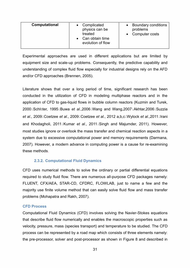
Table 3: Advantages and Disadvantages of the different Fluid Dynamic Approaches (Ekambara, 2005; Brennen, 2005)
Approach Advantages Disadvantages Experimental More realistic
Applications are possible
Equipment required Scaling problems Measurement
difficulties Operating costs
Analytical Clean, general information in formula form
Limited to simple geometry and physics
Restricted to linear problems
31
Computational Complicated physics can be treated
Can obtain time evolution of flow
Boundary conditions problems
Computer costs
Experimental approaches are used in different applications but are limited by
equipment size and scale-up problems. Consequently, the predictive capability and
understanding of complex fluid flow especially for industrial designs rely on the AFD
and/or CFD approaches (Brennen, 2005).
Literature shows that over a long period of time, significant research has been
conducted in the utilization of CFD in modeling multiphase reactors and in the
application of CFD to gas-liquid flows in bubble column reactors (Kuzmin and Turek,
2000;Schlüter, 1995;Buwa et al.,2006;Wang and Wang,2007;Akhtar,2006;Suzzia
et al., 2009;Coetzee et al., 2009;Coetzee et al., 2012 a,b,c;Wylock et al.,2011;Irani
and Khodagholi, 2011;Kumar et al., 2011;Singh and Majumder, 2011). However,
most studies ignore or overlook the mass transfer and chemical reaction aspects in a
system due to excessive computational power and memory requirements (Darmana,
2007). However, a modern advance in computing power is a cause for re-examining
these methods.
2.3.2. Computational Fluid Dynamics CFD uses numerical methods to solve the ordinary or partial differential equations
required to study fluid flow. There are numerous all-purpose CFD packages namely:
FLUENT, CFX/AEA, STAR-CD, CFDRC, FLOWLAB, just to name a few and the
majority use finite volume method that can easily solve fluid flow and mass transfer
problems (Mohapatra and Rakh, 2007).
CFD Process Computational Fluid Dynamics (CFD) involves solving the Navier-Stokes equations
that describe fluid flow numerically and enables the macroscopic properties such as
velocity, pressure, mass (species transport) and temperature to be studied. The CFD
process can be represented by a road map which consists of three elements namely:
the pre-processor, solver and post-processor as shown in Figure 8 and described in

32
detail below (Hung et al., 2007; Garcia et al., 2008).
Pre- processor
Creation of geometry Mesh generation Material properties Boundary conditions
SolverGoverning equations solve on a mesh
Transport equations
Mass Momentum
Physical models
Laminar
Solver settings
Initialisation Solution control Monitoring solution Convergence criteria
Post- processor
Velocity fields Pressure fields Concentration profiles
Figure 8 : The inter-connectivity functions of the three main elements within a CFD
analysis
2.3.2.1. Pre-processor
The first step in any CFD analysis regardless of the type of fluid flow begins with
creating the geometry, geometry parameters, domain shape and size (Garcia et al.,
2008). The domain geometry created requires mesh generation which can either be
structured or unstructured (Peraire et al., 1989; Baker, 2005; Thompson et al., 1998;
Samareh, 2005). The mesh has nodes at each cell and the solution obtained can be
improved by mesh refinements (number of cells). More cells mean improved
accuracy but higher computational costs and hence long calculation turnover times.
Hence, there always exists a trade-off between accuracy and turnover time (Tu et al.,
2008).
Once the geometry and mesh are defined, the next step is to set up the material
properties that are unique to a particular fluid flow system. The simulation is then
classified according to the following (Garcia et al., 2008):
Steady state/unsteady state flow
Compressible/incompressible
Laminar/turbulent flow regime
Together with the boundary conditions, there is in principle sufficient data to solve the
partial differential equations. For fluid flow, inflow and outflow boundary conditions
are required to explain the fluid behavior when entering or leaving the created flow
geometry.

33
2.3.2.2. Solver
The solver is used to solve the discretized governing equations which consist of the
mass, momentum, energy and other transport equations described below. The
Navier-Stokes equations which have been used for decades describe fluid flow by
assuming that fluid behaves as a continuum rather than as discrete particles
(MacCormack and Baldwin, 1975; Lohner, 2001; Crumpton et al., 1997; Burnett,
1987; Tu et al., 2008).
Mass equations The principle of conservation of mass states that mass can neither be destroyed nor
created. This principle is combined with the Gauss’s divergence theorem to an
arbitrary fixed volume in space for a compressible fluid yielding Eq. 16. This equation
describes the mass flux in and out of a fixed volume (can be fixed in space or move
with the fluid) where the change of mass with time is equal to the convective flux
ignoring any change in mass (Irani and Khodagholi, 2011).
Equation 16 can rearranged to Equation 16b using the material derivative of the
density field in Equation 16a.
For an incompressible fluid where the density is assumed to be constant, Equation
(16) reduces to Equation (17) below.

34
Momentum equations
The momentum equations can be derived from Newton’s second law of motion which
states that the rate of change of momentum equals the sum of forces acting on the
fluid. There are two sources of force acting on the moving fluid which are body forces
and surface forces. The body forces result from the location of the control volume in a
force field whereas the surface forces are due to interactions between the control
volume fluid and its surroundings. Therefore, the momentum balance for a control
volume can be represented by Equation 18 below (Tu et al., 2008).
+
Further evaluation of this equation with the assumptions of incompressible flow, and
Newtonian fluid flow yields the Navier-Stokes equation shown in Equation 19 (Clift et
al., 1978).
(19)
Analytical solutions to these equations can be obtained only under severely
restrictive assumptions. For example, the creeping flow approximation is derived by
neglecting the inertia terms of the Navier-Stokes equation and applies only to very
low Reynolds’s number Re < 0.1. However, most practical applications operate at
moderate to high Re (150 < Re < 270) hence the need to engage with CFD. This
then requires that accurate solutions are obtained by numerical solution of the full
Navier-Stokes equation (Clift et al., 1978).
Three discretization methods can be used to solve the governing equations, namely:
finite difference, finite volume/element and spectral methods. The advantages and
disadvantages of the different methods are listed in Table 4 below.

35
Table 4: Advantages and Disadvantages of the different discretization methods (Kumar, 2009)
Method Description Advantages Disadvantages
Finite Difference
Finds discrete solutions on a grid/mesh
Simple Complicated Domains Discretized classical
solutions Finite Element/ Volume
Based on a partition of the domain into small finite elements
Better in irregular domains
More complex to set up and analyze
Spectral Methods
Solutions are approximated by a truncated expansion in the eigenfunction of some linear operator.
Highly accurate for problems with smooth solutions
Not so useful on irregular domains or for problems with discontinuities
The finite volume method is favourable to this research because of its applicability to
arbitrary geometries, structured and unstructured meshes and its local conservation
of numerical fluxes. This makes the finite volume technique very attractive when
modelling problems where flux is important as is the case in the proposed work to
predict average mass transfer coefficients (Eymard et al., 2006).
2.3.2.3. Post-processing and Analysis
The last step in the CFD process is the post-processor which involves collecting the
required output be it in the form of velocity, pressure or concentration profiles. The
analysis of the data collected is done to explain results for the research study (Hung
et al., 2007; Garcia et al., 2008).
2.4. Macro Modelling The previous section discussed the mass transfer between the fluid and a single
bubble (micro-modelling). The mass transfer mechanism in the entire Bubble Column
can be simulated through the use of Multiphase CFD techniques. When modelling
multiphase flows, there are two common approaches, namely, the Euler-Lagrange
and Euler-Euler approaches. These models have shown that the CFD predictions for

36
the entire bubble column is at a reliable level since solutions from them have been in
good agreement with experimental macroscopic flow properties in bubble columns
(Becker et al., 1994).
2.4.1. The Euler-Lagrange Approach
In this approach, the fluid phase is treated as a continuum by solving the time-
averaged Navier-Stokes equations, while the dispersed phase is solved by tracking a
large number of particles, bubbles, or droplets through the calculated flow field
(Delnoij et al., 1997). The dispersed phase can exchange momentum, mass and
energy with the fluid phase. A fundamental assumption made in this model is that the
dispersed second phase occupies a low volume fraction, even though a high mass
loading (the mass of particle is greater than equal to the mass of the fluid) is
acceptable (Kumar, 2009).
The particle or droplet trajectories are computed individually at specified intervals
during the fluid phase calculation. This individual computation makes the model
appropriate for the modeling of spray dryers, coal and liquid fuel combustion and
some particle laden flows, but inappropriate for the modeling of liquid-liquid mixtures,
fluidized beds or any application where the volume fraction of the second phase is
not negligible (Mohapatra and Rakh, 2007). In summary, this approach solves the
flow field by computing each individual bubble by considering the bubble-bubble and
bubble-liquid interactions. (Zhang et al., 2007)
2.4.2. The Euler-Euler Approach
In the Euler-Euler approach, the different phases are treated mathematically as
interpenetrating continua (Delnoij et al., 1997). The volume of a phase cannot be
occupied by the other phase; Hence the introduction of the volume fraction concept.
This means that the bubble size is represented by the volume fraction (Zhang et al.,
2007).
37
These volume fractions are assumed to be continuous functions of space and time
and their sum is equal to one. Conservation equations for each phase are derived to
obtain a set of equations, which have similar structure for all phases. These
equations are closed by providing constitutive relations that are obtained from
empirical information or, in the case of granular flows, by application of kinetic theory
(Kumar, 2009). This approach is limited because it must be coupled with the
population balance to obtain more information on the bubble size distribution (Zhang
et al., 2007).
Some other CFD Methods have been recently developed such as the Large Eddy
Simulation (LES) and Direct Numerical Simulation (DNS) (Apte et al., 2004; Mahesh,
2006). For example, the DNS approach requires closure models and is only
practically applicable to a finite number of bubbles and limits the simulation of other
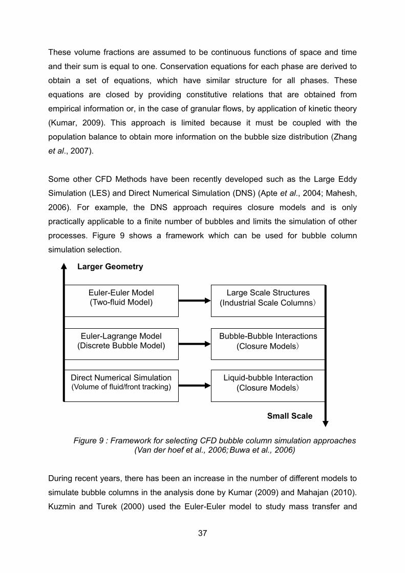
processes. Figure 9 shows a framework which can be used for bubble column
simulation selection.
Figure 9 : Framework for selecting CFD bubble column simulation approaches (Van der hoef et al., 2006; Buwa et al., 2006)
During recent years, there has been an increase in the number of different models to
simulate bubble columns in the analysis done by Kumar (2009) and Mahajan (2010).
Kuzmin and Turek (2000) used the Euler-Euler model to study mass transfer and
Euler-Euler Model (Two-fluid Model)
Large Scale Structures (Industrial Scale Columns)
Euler-Lagrange Model (Discrete Bubble Model)
Bubble-Bubble Interactions (Closure Models)
Direct Numerical Simulation (Volume of fluid/front tracking)
Liquid-bubble Interaction (Closure Models)
Larger Geometry
Small Scale

38
chemical reaction for gas-liquid flows in Bubble Columns. The computational results
showed the implications of reaction enhanced mass transfer in bubble columns and
called for more grounds to continue research in this field.
Schlüter (1995) used the BCR computer code, a modular structured computer
program to simulate steady state bubble columns. The code can be used for different
options by determining the local pressure, temperature and concentration profiles
over the column height. However, there is little information on the validation of the
BCR model.
Buwa et al. (2006) experimentally validated the Eulerian-Langrangian models and
gathered useful data for the simulation of mass transfer and reactions in bubble
columns. Akhta (2006) validated the simulation of a bubble column against
experimental results with different distributors using the Two-fluid Eulerian model.
The influence of different distributors on the hydrodynamics of the system was
investigated.
Wang and Wang (2007) used the Computation Fluid Dynamics–Population Balance
Model (CFD–PBM) coupled model to simulate bubble columns. The
simulation results showed that the CFD–PBM is an efficient method for predicting the
hydrodynamics, bubble size distribution, interfacial area and gas–liquid mass
transfer rate in a bubble column. This is a good method of simulation because it
evaluates the bubble size in the column which is an important aspect in improving
bubble column simulation.
Suzzia et al. (2009) validated the use of Euler-Euler and Euler-Lagrange approaches
to simulate bubble columns. The Euler-Euler approach showed promising results for
coarser mesh sizes and the Euler-Lagrange approach proved to be a more advance
method for simulation. Zhang et al. (2008) continued to use the Euler-Euler model to
simulate mass transfer and chemical reaction in a bubble column.
Coetzee et al., (2009) developed a rapid evaluating semi analytical model called the
Bubble Cell Model (BCM). The BCM provides the steady state velocity and pressure

39
fields around individual bubbles as a function of Reynolds number (Figure 10). BCM
is dependent on the Re number of the bubble and avoids the use of closure models
while providing micro structure flow information (Coetzee et al., 2012).
The main BCM advantages over other models are as follows (Kumar, 2009; Mahajan
2010):
The solving of complex PDEs in the regions around the bubble is avoided
Small scale flow information is provided by the cell model
Rapid evaluation compared to conventional techniques (Euler-Euler and Euler-
Lagrange)
Figure 10 : Velocity vector fields around an individual generated in the BCM
Coetzee et al. (2012, a, b, c) adapted the BCM to a macro fluid model such that the
entire bubble column could be simulated. It was constructed by extending the range
of the creeping and potential flow analytical solutions by incorporating a stochastic
model. This model accounts for deviations from the analytical solutions that is, flow
separation and the non-linear wake feature.
Wylock et al. (2011) used the Direct Numerical Simulation approach to simulate
bubble mass transfer with chemical reaction and showed that there is a clear
difference between the 1D and 2D models. The results from the study by Irani and

40
Khodagholi (2011) showed that simple two dimensional models cannot be used in
engineering calculations required in the design of bubble columns.
Kumar et al. (2011) validated the two and three phase up-flow in a bubble column
with experimental values and obtained axial liquid velocity profiles. Singh and
Majumder (2011) studied the co and counter-current mass transfer in bubble columns
using a mechanistic model to predict mass transfer efficiency. It was suggested that
the concentration variation may be useful for future understanding of the mass
transfer phenomena in bubble column reactors.
2.5. Summary The development of numerous CFD models used in the simulation of bubble columns
has gradually increased in recent years. Considerable work has been accomplished
in the understanding of bubble columns characteristics depending on the size and
scale (Kumar, 2009; Mahajan 2010). In general, studies have shown that the different
models are unique and limited to a practical system (Kuzmin and Turek,
2000;Schlüter, 1995;Buwa et al., 2006 ;Wang and Wang ,2007;Akhtar, 2006
;Suzzia et al., 2009;Coetzee et al., 2009 ;Coetzee et al., 2012 a, b, c ;Wylock et al.,
2011 ;Irani and Khodagholi, 2011 ;Kumar et al., 2011;Singh and Majumder, 2011).
Models are validated to ensure that the modeled system is appropriately predicted.
Some models however are purely theoretical while others have been experimentally
validated (Schlüter, 1995; Wang and Wang, 2007; Coetzee et al., 2009; Coetzee et
al., 2012 a, b, c).
It is worth noting that many studies are trying new approaches and drifting away from
the common Euler-Euler and Euler-Lagrange models in favor of greater
computational efficiency (Wang and Wang, 2007; Coetzee et al., 2009 ;Coetzee et
al., 2012 a, b, c). Models like the Direct Numerical Simulation are now frequently
used for bubble column simulation but still rely on closure models (Wylock et al.,
2011). The CFD-PBM is appropriate for analyzing bubble size in detail (Wang and
Wang, 2007).

41
Studies have shown that the mass transfer coefficients can be predicted using the
CFD approach that requires closure models. However, there is still a gap in the
fundamental understanding of the mass transfer and chemical reaction properties. It
is not clear which is the most appropriate and less computationally expensive CFD
approach to investigate mass transfer and chemical reaction.

42
Chapter 3 Motivation and Objectives
3. Motivation and Objectives In this study, a fast-solving semi-analytical model called the Bubble Cell Model (BCM)
proposed by Coetzee et al., (2009; 2012 a, b, c) is used to simulate gas-liquid flows
around individual bubbles in a bubble column. This model provides an alternative
multiphase modeling approach and substitutes the conventional closure models with
a statistical model of the micro flow structure.
Many mass transfer experiments have been carried out in the literature but each of
these sets of results are very specific to the chemical system, equipment type and
operating conditions. Therefore, a more general method is needed to predict kl from
fundamental principles in a computationally inexpensive way.
The Bubble Cell Model (Coetzee et al., 2009; 2012 a, b, c) approach in its current
state simulates the steady state velocity and pressure fields that develop in the
immediate vicinity of individual bubbles. At present, the BCM incorporates only the
local velocity vector field and does not predict the concentration field. As such, the
model cannot be used in the present form to predict mass transfer rates or local
reaction rates.
The concentration field can be predicted by coupling the mass balance to the
momentum balance in the BCM. These concentration lines will show how the film
thickness varies axisymmetrically around the bubble, hence, allowing for prediction of
the mass transfer rates in the system.
The objective of the present study is therefore to extend the BCM to mass transfer
applications. This model uses the film theory to calculate kl for a homogeneous
nitrogen-water system as a function of the Re and Sc numbers. As a significant
outcome, such a model would be used to reliably predict the average mass transfer
coefficients in a bubble column rather than through empirical correlations and
experiments.

43
Hypothesis
The hypothesis of the present study is that “the average mass transfer
coefficient in a bubble column can be reliably predicted as a function of
Reynolds number (Re) and Schmidt number (Sc) by coupling a material balance
to a Bubble Cell Model.”
Key Questions These questions will aid in either proving or disproving the hypothesis and are as
follows:
1. How will the mass boundary layer thickness be averaged around bubble?
2. What is the impact of the Reynolds and Schmidt numbers on the average
mass transfer coefficients?

44
Chapter 4 Model Development
4. Model Development
4.1. Model Geometry
In an industrial environment, bubble columns usually operate in turbulent regimes
where Re > 1000 due to the high level of contact associated with strong mixing. The
turbulent regime is complex due to the multiphase hydrodynamics (bubble-bubble
interactions) that result in varying bubbles shapes. These varying shapes are an
output of either increasing or decreasing the Reynolds, Morton and Eötvös numbers
as described in section 1.1.1. Figure 11 illustrates the formation of the different
shapes with respect to Re, Eo and Mo, the spherical bubble shape is observed
before deformation to other oblate ellipsoidal and spherical cap shapes.
Figure 11: Typical bubbles shapes in aqueous sugar solutions (Bhaga & Weber,
1981)

45
*S: Spherical, OE: oblate ellipsoidal, OED: oblate ellipsoidal disk, OEC: oblate ellipsoidal cap, SCC: spherical cap, closed wake, SCO: spherical cap, open wake, SKS: skirted, steady
skirt, SWS: skirted, wavy skirt.
Experimental investigations have shown that flow changes dramatically with
increasing Reynolds number. In order to obtain a steady axisymmetric and steady
planar-symmetric flow regime, the Reynolds number lies in the different ranges
respectively 20 < Re <210 and 210 < Re <270 (Taneda,1956,1978; Wu,1993;
Natarajan,1993; Nakamura,1976; Margavey and Bishop, 1961). It is clear from Figure
11 that increasing the Re makes the flow more complex with varying bubble shapes.
For simplicity, the present study was limited to a steady state flow regime with Re ≤
270 and simulate only flow over a spherical bubble shape.
In a bubble column, fluid flowing around the moving bubbles in the entire column can
be modelled most intuitively using a moving frame of reference. An alternative way of
modelling is to fix a stationary bubble in the column and track the relative velocity
between the fluid and the bubble. In this present study, the bubble is assumed to be
stationary and the bubble size does not change as the fluid flows over the bubble
surface. In practice, the velocity vector field is supposed to change since the bubble
dissolves (Ponoth and McLaughlin, 2000); the velocity field was assumed to be
steady as in the case of a bubble at its terminal velocity.
4.1.1. Mesh Generation In order to simulate the fluid flow over a spherical bubble as assumed above, a good
quality mesh is generated using the software called Gambit. Gambit software is used
for meshing applications where it defines the domain geometry and generates the
mesh grid.
A two dimensional axisymmetric grid is used under the assumption that there are no
velocity gradients in the angular direction. For spherical coordinates, the points are
referenced as (r, θ, ) but with the axisymmetric condition, gradients with respect to
are zero. Therefore the geometry axisymmetrically revolves around the x-axis of the
domain alongside with the two dimension grid makes the Navier stokes equation
easier to solve and requires less time to solve and is thus more computationally

46
efficient.
A two dimensional axisymmetric rectangular mesh grid of width 0.025m, height
0.015m and triangular structured mesh elements is used for the simulation with a
bubble of diameter d= 0.005m. Using the general accepted rules of thumb in the field
of CFD modelling (Thompson et al., 1998), the spherical bubble is located 10xd away
from the inlet walls so that wall effects on the sphere are negligible.
The typical boundary conditions for the mesh grid; velocity inlet, outlet, wall, axis, and
the bubble wall are implemented in the mesh generation to describe the required flow
pattern. Additionally, the conditions of the simulation are provided as follows:
Velocity inlet - The Dirichlet boundary condition involves specification of the
inlet velocity as stated in Equation 19. The inlet velocity was varied from
0.02675 to 0.2408 m s-1 corresponding to the Reynolds number range of 30 to
270 for laminar flow at 298.15K.
Outflow - In this case, there is no pressure or velocity specification since the
solution at the outlet is extrapolated from the interior. The outflow boundary,
which is intended for incompressible flow and is also where mass balance
correction is applied.
Bubble - A nitrogen mass fraction of was specified for the species
boundary condition. The calculation of the mass fraction is explained in section
6.1. It has been shown that the boundary condition on a bubble in a
contaminant free system corresponds to a zero-shear-stress one, rather than
a no-slip boundary condition, which would be applicable to rigid particles
(Hadamard, 1911). Vasconcelos et al. (2002) also showed that surfactants
affect the mass transfer rates and bubbles to behave like solid spheres. It is
therefore assumed that there are no contaminants in the liquid and that the
interfacial tension is constant
Wall - The walls are also assumed to be stationary with no flux of species
(zero diffusive flux). This is because, these walls do not represent the actual

47
walls of a bubble column, but are only used to create a computational domain
where the fluid around the bubble is bound. Therefore, the effects of the
confining wall are neglected and zero-shear-stress (free-slip) condition is
applied.
Figure 12 illustrates the axisymmetric geometry which is finer closer to the bubble
and coarser in the outer region. Meshes are made finer in the regions where there
are large variations from node to node and enable the gradients of velocity and
concentration near the sphere to be resolved numerically.
Figure 12: Axisymmetric grid and mesh generation around spherical bubble
4.1.2. Mesh Optimization
It is required of any CFD simulation that the solution be converged and independent
of the resolution of the mesh. Mesh quality is usually measured by the grid skewness;
Equisize Skew and EquiAngle Skew, smoothness and aspect ratio (Thompson et al.,
1998; Lee et al., 1991; Silva et al., 2011; You et al., 2006).
Mesh quality simply means, the ability of the mesh to capture and improve resolution
of all relevant features without increasing the computational effort. An acceptable
mesh must have low skewness, smooth change in size and an aspect ratio of one in
order to be accurate. The difference between an element with low and high skewness
is shown below in Figure 13.

48
Figure 13: An Element with low skewness (left) and high skewness (right)
Depending on the cell geometry, the desired situation is obtained when majority of
the cells are found with Equisize Skew and EquiAngle Skew values between 0 and
0.7 respectively. Most often, a tetrahedral mesh does not meet this criterion (Silva et
al., 2011).
Different mesh grids with different mesh faces are generated and simulated in order
to get the mesh grid which is independent of the solution. Finally, a mesh size with
approximately mesh faces and 100% of the cells within the Equisize Skew
range is chosen as the grid used for the entire simulation process.
4.2. Model System The BCM developed in Coetzee et al., (2009), simulates the immediate flow regions
around individual bubbles in a Bubble column from the Reynolds number using an
algebraic flow model. In other words, the BCM is a hybrid between analytical and
statistical methods which improves the simulation accuracy and reduces the number
of parameters of the flow model by solving the Navier-stokes equation over a fixed
spherical bubble.
The discretization schemes for solving the governing equations was the Second-
order Upwind whereas the pressure-velocity coupling scheme was Phase Coupled
SIMPLE in Fluent 13.0. The SIMPLE scheme is a standard pressure correction
algorithm for finite volume calculations and is adequate for incompressible viscous
flow. This scheme was chosen because it minimizes the false diffusion presented in

49
other interpolation techniques such as the first order upwind. (Tu et al., 2008;
Pantankar, 1980)
The parameters for the BCM are estimated in two fitting stages as shown in Figure
14 below. Stage one involves fitting every steady state velocity vector field with
respect to the radial and angular coordinates at a specified Reynolds number range.
Stage two involves the cross correlation of stage one model with respect to Reynolds
number.
In simpler terms, in stage one the BCM parameters are fitted for any given Reynolds
number while in stage two, the BCM parameter is varied in Reynolds number and a
model is proposed for each parameter as a function of Reynolds number. This
enables the entire velocity vector field to be generated when given only the Reynolds
number.

50
Figure 14: BCM fitting stage strategy where are the overall stage one model, stage one parameter, stage two model and parameters respectively (Coetzee
et al.,2009)
Re
CFD:
Stage One:
Estimate
Stage Two:
Estimate
BCM:
For all Re
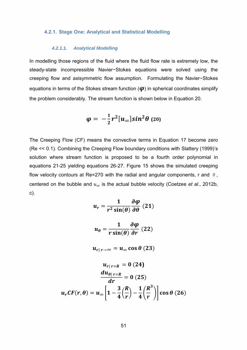
51
4.2.1. Stage One: Analytical and Statistical Modelling
4.2.1.1. Analytical Modelling
In modelling those regions of the fluid where the fluid flow rate is extremely low, the
steady-state incompressible Navier−Stokes equations were solved using the
creeping flow and axisymmetric flow assumption. Formulating the Navier−Stokes
equations in terms of the Stokes stream function ( ) in spherical coordinates simplify
the problem considerably. The stream function is shown below in Equation 20.
(20)
The Creeping Flow (CF) means the convective terms in Equation 17 become zero
(Re << 0.1). Combining the Creeping Flow boundary conditions with Slattery (1999)’s
solution where stream function is proposed to be a fourth order polynomial in
equations 21-25 yielding equations 26-27. Figure 15 shows the simulated creeping
flow velocity contours at Re=270 with the radial and angular components, r and θ,
centered on the bubble and is the actual bubble velocity (Coetzee et al., 2012b,
c).
24)

52
(27)
Figure 15: Velocity vector fields around bubble in Creeping Flow at Re=270 (Coetzee et al., 2012b, c)
The opposite extreme to creeping flow is inviscid flow meaning a fluid with no
viscosity. Zero viscosity fluids do not exist; however, the assumption provides a good
description of the velocity profile except near the body and beyond the line of flow
separation. The velocity potential, Φ, is defined such that Φ, the free slip
boundary condition, upon differentiation yields Potential Flow (PF) velocities in
equation below 28-29. It should be noted that Potential Flow as follows from Equation
17 is when the viscous terms are zero and Reynolds numbers goes to Infinity
(Coetzee et al., 2012b, c).
The simulation carried out with the Potential flow conditions yields the solution shown
in Figure 16. A complete solution from the Navier stokes equations simulated in CFD
illustrated in Figure 17 (Coetzee et al., 2012b, c).

53
(29)
Figure 16: Velocity vector fields around bubble in Potential Flow at Re=270 (Coetzee
et al., 2012b, c)
Figure 17: Velocity vector fields around bubble from complete simulation of Navier-
Stokes Equations at Re=270 (Coetzee et al., 2012b, c)

54
Under these assumptions, simple analytical solutions in the form of algebraic
expressions result; these forms can be rapidly evaluated and incur minor
computational expense. Unfortunately, the analytical solution is not able to capture
the flow separation and wake features at the rear of the bubble, which occur at very
low Reynolds number. Therefore, the analytical model cannot predict flow at the rear
of the bubble and limits its applicability for hydrodynamic calculations (Coetzee et al.,
2012b, c).
4.2.1.2. Statistical Modelling
The two extreme conditions in modeling fluid flow are creeping and potential
(Inviscid) flow models where ; are combined to account for
accurate flow structure in any flow regime. The stage one parameters, ij, are
defined such that i is either the radial or angular coordinate and j, the type of flow
model. The linear combination of the two solutions is shown in Equation 30-31 where
are the weighting coefficients obtained through linear least squares with
respect to the true velocity, (Coetzee et al., 2012b, c).
The residuals for the nonlinear data in Equations 30 and 31 are evaluated using the
regression with Empirical modelling strategy. An accurate CFD computational
solution is characterized by convergence of the iterative process, the grid
independence and the use of acceptable solution methods. The grid independence
justifies the grid choice for simulation. The convergence of the iterative process is
obtained by calculating the imbalances, called residuals, in the algebraic equations.
Residuals can be viewed as estimates of computational errors that indicate how
accurate the results are. Accurate results further indicate that the system has
reached quasi-steady state. Once this state is achieved, average quantities are
calculated in terms of the time, axial and radial coordinates. It should be noted that
Fluent 13.0 is a deterministic model and therefore does not have any experimental
errors coupled with it.

55
4.2.1.2.1. Empirical Method The residuals of the radial and angular velocity are treated by fitting the residual
velocity surfaces across the Reynolds operating range and identifying where simple
functions can form residuals to the solution. The symmetry at x=0 helps to simplify
the problem (Coetzee et al., 2012 b, c).
The residual of the radial velocity in Equation 32 was basically in the bubble wake
region and by identifying the critical angle and the final model had 17 parameters
(Figure 18; Coetzee et al., 2012b, c). The residual of the angular velocity in Equation
33 was at maximum at the bubble surface which decayed into the radial direction and
had 11 parameters left to be solved (Figure 19; Coetzee et al., 2012b, c).
Figure 18: Radial residual around bubble (Coetzee et al., 2012b, c)
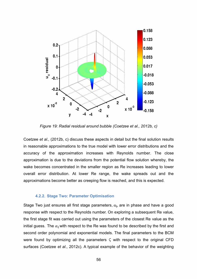
56
Figure 19: Radial residual around bubble (Coetzee et al., 2012b, c)
Coetzee et al., (2012b, c) discuss these aspects in detail but the final solution results
in reasonable approximations to the true model with lower error distributions and the
accuracy of the approximation increases with Reynolds number. The close
approximation is due to the deviations from the potential flow solution whereby, the
wake becomes concentrated in the smaller region as Re increases leading to lower
overall error distribution. At lower Re range, the wake spreads out and the
approximations become better as creeping flow is reached, and this is expected.
4.2.2. Stage Two: Parameter Optimisation Stage Two just ensures all first stage parameters, ij, are in phase and have a good
response with respect to the Reynolds number. On exploring a subsequent Re value,
the first stage fit was carried out using the parameters of the closest Re value as the
initial guess. The ij with respect to the Re was found to be described by the first and
second order polynomial and exponential models. The final parameters to the BCM
were found by optimizing all the parameters with respect to the original CFD
surfaces (Coetzee et al., 2012c). A typical example of the behavior of the weighting

57
coefficients is shown in Figure 20 (Coetzee et al., 2012b).
Figure 20: Second Stage Fit of parameters (Coetzee et al., 2012b)
4.2.3. BCM Development The creeping and potential flow analytical solutions discussed in the Section 4.2.1.1
provide good approximations and explain some significant areas of the velocity flow
field around the bubble for Re ≤270. Unfortunately these analytical solutions do not
describe clearly the flow at the rear of the bubble especially at Low Reynolds
Numbers.
On the other hand, statistical/Empirical models also gave good fits. Any statistical
model must accurately account for deviations from analytical solutions, flexible for
any data or bubble shape and require a sensible amount of parameters.
A hybrid between analytical solutions and statistical models has been investigated
and gives accurate approximations. Figure 21 and 22 illustrate individual models, the
simulated results from combining both models for appreciation and comparison with
CFD data are validated.
Therefore, a new approach was been developed by Coetzee et al. (2009) to simulate
bubble columns derived by combining the analytical and statistical modeling solutions
to obtain steady state velocity field vectors over a sphere (Coetzee et al., 2012b).

58
(a) Semi-Analytical Model for Radial Co-ordinates
(b) Statistical Model for Radial Co-ordinates

59
(c) Semi-Analytical and Statistical Model for Radial Co-ordinates
(d) Original CFD Data for Radial Co-ordinates
Figure 21: Comparison of Semi-analytical, Statistical, Semi-analytical and Statistical models with Original CFD Data for Radial Co-ordinates (Coetzee et al., 2012b)

60
(a) Semi-Analytical Model for Angular Co-ordinates
(b) Statistical Model for Angular Co-ordinates

61
(c) Semi-Analytical and Statistical Model for Angular Co-ordinates
(d) Original CFD Data for Angular Co-ordinates
Figure 22: Comparison of Semi-analytical, Statistical, Semi-analytical and Statistical models with Original CFD Data for Angular Co-ordinates (Coetzee et al., 2012b)

62
Chapter 5 Mass Transfer Extension to the BCM 5. Mass Transfer Extension to the BCM
The flow around the bubble surface is analyzed by using the BCM developed by
Coetzee et al. (2009, 2012a, b, c) which predicts the velocity vector fields around
single bubbles in bubble column reactors. This model lacks the ability to predict
average mass transfer coefficients; therefore a material/species balance capable of
predicting the concentration field in the vicinity of the bubble is integrated into the
model. The ANYSY CFX computer package (Fluent 13.0) is used to develop the
simulation. The computer package uses the finite volume technique which generates
the flux in its numerical solutions. The overall outcome is achieved by running several
CFD simulations. The CFD results are then used to identify the average boundary
layer which can then be used to determine the mass transfer coefficient.
5.1. Mass Transfer from Sphere
Mass transfer from a sphere to a flowing fluid applies the steady state transport
equation (Navier-stokes and diffusion equations) shown below in Equation 34. This
transport equation is derived by assuming constant diffusivity with no chemical
reaction and is dependent on velocity.
The concentration in the sphere, Co, remains constant and is assumed to be
negligible compared to the overall concentration in the system. The concentration
diffused to the external flowing stream is C1. Equation 34 in its dimensionless form is
Equation 35 and rearranging yields Equation 36 in terms of the cylindrical co-
ordinates (Finlayson, 1972).
For negligible internal resistance and constant concentration in the sphere, the
boundary conditions are Equations 37-40 (Clift et al., 1978)
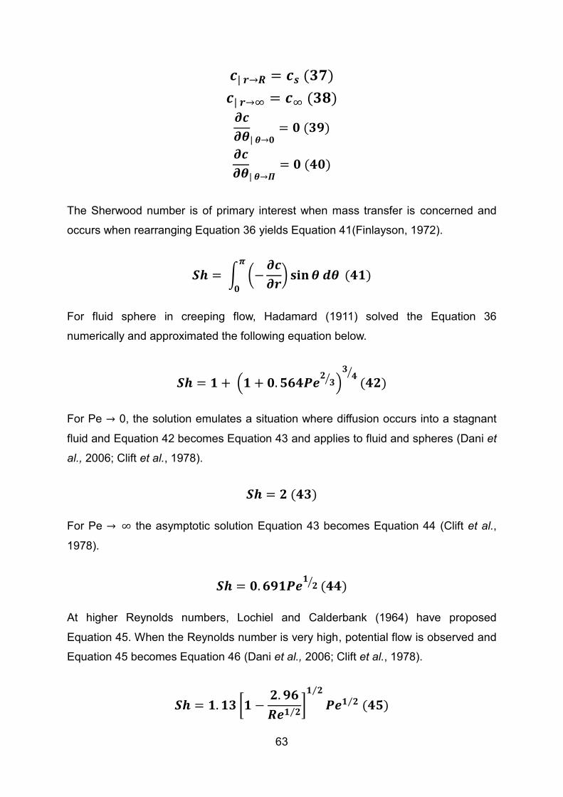
63
The Sherwood number is of primary interest when mass transfer is concerned and
occurs when rearranging Equation 36 yields Equation 41(Finlayson, 1972).
For fluid sphere in creeping flow, Hadamard (1911) solved the Equation 36
numerically and approximated the following equation below.
For Pe 0, the solution emulates a situation where diffusion occurs into a stagnant
fluid and Equation 42 becomes Equation 43 and applies to fluid and spheres (Dani et
al., 2006; Clift et al., 1978).
For Pe the asymptotic solution Equation 43 becomes Equation 44 (Clift et al.,
1978).
At higher Reynolds numbers, Lochiel and Calderbank (1964) have proposed
Equation 45. When the Reynolds number is very high, potential flow is observed and
Equation 45 becomes Equation 46 (Dani et al., 2006; Clift et al., 1978).

64
It should be pointed out that these Equations shown above are attempts derived from
first principles and not from actual simulations. Dani et al., (2006) developed
equations from actual simulations on a spherical bubble with results agreeing to the
film theory. However, their accuracies are to be put under scrutiny since the
equations are empirical.

65
Chapter 6 Model Simulation
6. Model Simulation
6.1. Input and Output Parameters The most important aspect of the simulation is the incorporation of the material
balance into the fluent solver. For a basic fluid flow, only the species transport is used
with no inlet diffusion and energy source. The materials required for the mass
balance are selected and specific parameters such as; viscosity, density and mass
diffusivity for the mixture are defined.
A non-reactive steady state nitrogen-water system is chosen to predict the mass
transfer coefficient as a function of Re and Sc numbers. The velocity and mass
diffusivity of nitrogen gas into liquid water are the only changing variables in the
definition of Re and Sc numbers respectively. It should be noted that the mass
diffusivity of water into nitrogen is assumed to be negligible in the present study.
The inlet velocity and species mass fraction, species mass diffusivity are imported
into the CFX computer package (Fluent 13.0) and solved mathematically to get
simulated results. Upon validation, the applications can later be extended to reactive
systems. The physical properties of nitrogen-water system are shown in the Table 5
below. An incompressible laminar isothermal steady state process in two-dimensional
flow is used for the research study.
Table 5: Physical Properties of Nitrogen and Water at 293.15K and 1atm
Properties Nitrogen (gas)
Water (liquid) References
Density, (kg/m3) 998.2 Weast,1988
Diffusivity, ( 2.36
Sada et al,1975
1.88 Cussler, 2003 2.01 Ferrel and Himmelblau,1967
Viscosity, 1000 Weast,1988 A nitrogen mass fraction of at 25°C and 1 atm was derived from the product
of N2 Saturated concentration solubility in water (Henry‘s Law) at 0.625 mol/m3 and

66
the molar mass of nitrogen is kg/mol. This product yields a mass per volume
of and density of water, 998.2 kg/m3.
Fluent 13.0 can simulate various operating conditions such as, laminar and turbulent
flows, steady or unsteady states systems. The governing equations from the
particular system are converted into algebraic equations. The discretization scheme
is selected and formulates the equations on every location on the domain grid. The
equations are then iterated over the domain until a converged solution is attained.
6.2. Species Transport Simulation
1. Mesh
Firstly, the axisymmetric mesh grid as shown in Figure 12 is imported into Fluent
13.0. The mesh scale is then verified to ensure that there is no difference in
dimensions between Gambit and Fluent 13.0. The mesh grid is checked for co-
ordinates, volume and face statistics such as the number of nodes per cell, face cells
and so on. Even though, the mesh quality has been guaranteed in Gambit, Fluent
13.0 still gives a breakdown of the mesh skewness, smoothness and aspect ratio.
After all these procedures, the grid is ready to be displayed with the grid conditions.
The pressure based solver is used with an absolute velocity formulation for the two
dimensional planar and steady state system. In this nitrogen-water system, a double
precision model was chosen because it resolves any pressure difference that drives
flow (driving force) in the geometry. The pressure based model is typically chosen for
incompressible flows (Tu et al., 2008).
2. Model Definition
This is the definition of the type of model and the mixture properties that is used in
the simulation. For a basic fluid flow, only the species transport model is used with no
inlet diffusion and energy source. The volumetric species for the mixture are
selected; in this case which are nitrogen and water in their pure states.
3. Materials
The nitrogen and water mixture and fluid composition have been defined with the

67
following properties; Density (kg/m3)– Incompressible ideal gas
Specific Heat Capacity (j/kg-k) – Mixing law
Thermal conductivity (w/m-k) – Constant (0.0454)
Viscosity (kg/m-s) – Constant (9.0796e-5)
Mass diffusivity (m2/s) – Constant-dilute-approximate (2.93e-5)
4. Boundary Conditions
The momentum and species boundary conditions defined in section 4.1.1 are now
integrated into the mesh grid. To summarise, the top and bottom walls are stationary
with the no slip shear condition and zero nitrogen diffusive flux. The outlet has zero
gauge pressure to induce a driving force. The inlet uses a magnitude, normal to
boundary velocity specification method and absolute reference frame. The constant
inlet velocity magnitude is inserted here. This is the point where the different
velocities will be inserted as the Reynolds number is varied. The nitrogen species
boundary condition is the specified mass fraction which is a constant defined in
section 6.1 above.
5. Reference Values
The reference values are computed from the inlet boundary condition since the inlet
velocity is being varied.
6. Solution Methods
Mass conservation within a flow domain is mainly accounted for by correct linkage of
pressure and velocity. This is taken into consideration by the solution procedures or
algorithms within the CFD codes (Tu et al., 2008). The discretization schemes for
solving the governing equations was the Second-order Upwind whereas the
pressure-velocity coupling scheme was Phase Coupled SIMPLE. This scheme was
chosen because it minimizes the false diffusion presented in other interpolation
techniques such as the first order upwind. The SIMPLE scheme is a standard
pressure correction algorithm for finite volume calculations and is adequate for
incompressible viscous flow.

68
7. Solution Controls
Under-relaxation factors assist in achieving a converged solution and moderate the
iteration process of the system of algebraic equations that govern fluid flow (Tu et al.,
2008). Default under-relaxation factors for pressure, density, body forces of 0.3, 1,
0.7 were used respectively and nitrogen mass fraction of . 8. Monitors
An accurate CFD computational solution is characterised by convergence of the
iterative process, the grid independence and the use of acceptable solution methods.
The grid independence justifies the grid choice for simulation as demonstrated in
Section 4.1.2. The convergence of the iterative process is obtained by calculating the
imbalances called residuals in the algebraic equations.
Residuals, in other terms, can be viewed as estimates of computational errors and
tell how accurate the results are. Accurate results also show that the system has
reached quasi steady state and once in this state, average quantities are calculated
in terms of the time, axial and radial coordinates.
9. Solution Initialization and Run Calculation
Finally, the solution procedure is initialized from the inlet conditions and the number
of iterations required is given. The equations are calculated until steady-state
converged concentration profiles are obtained as shown in Figure 24.
10. Simulation Results
A unique solution is reached when the residuals fall below certain convergence
criteria. The absolute criteria for continuity, x-y velocity and nitrogen concentration
are , respectively. Figure 23 shows the residuals converge after the
required number of iterations. It should be noted that FLUENT 13.0 is deterministic
model and therefore does not have any experimental errors coupled with it.
To simulate the different Reynolds numbers, only the corresponding inlet velocity is
changed in the model with the solution initialized. The nitrogen species molar
concentration contours around the bubble are generated and imported into Matlab.

69
Figure 23: Converged Results from simulation
11. Mass Transfer Results
Mass transfer occurs due to concentration gradients; for this reason concentration
profiles are generated. Once the CFD result is obtained, concentration profiles
around the bubble are analyzed in the form of concentration iso-surface or boundary
layer as in Figure 24. The identification of the species mass boundary layer thickness
is defined by the film theory, which as mentioned previously, is the point from the
bubble interface to 99% of the concentration of the diffusing component in the bulk
liquid.
6.3. Average Boundary Layer Calculations
The iso-concentration contours from the simulation converge to a long tail as seen in
Figure 24 and are clearly not uniform around the bubble; it is thinner at the front of
the bubble and wider at the rear of the bubble. The mass boundary layer thickness
around the bubble therefore, needs to be averaged to obtain a single representative
film thickness so as to estimate the average mass transfer coefficient.
To achieve this, the long tail as shown in Figure 25 is cut off and the mass boundary

70
layer thickness at each angle around the hemisphere of the bubble of the
axisymmetric axis are added and averaged as described in Equation 47.
Figure 24: Long Tail of Concentration Iso-surfaces around the bubble

71
Figure 25: Derivation of the Average Concentration boundary layer with r, radius of bubble and
To perform the cut-off so that the mass boundary layer thickness is averaged around
a bubble; a critical angle that exists where there is a point of flow separation is
identified. Beyond this critical angle, there is a high circulation zone where the
concentrations normalise such that there is no mass transfer driving force. Clift et al.
(1978) applied Equation 48 to describe this angle which applies to fluid flow over rigid
spheres and is in radians (20 ≤ Re ≤ 400).
Yan et al., (2002) actually explained this flow of separation with the layer around the
rigid sphere thicker than that of a fluid sphere. By analysis, it was showed that the
flow of separation near the rear encourages the development of a thicker boundary
layer in front of the actual separation point.
On the other hand, Dani et al., (2006) shows that the spherical symmetry obtained
around bubble at low Re occurs because the mass transfer is controlled by diffusion.
r
r+ r+

72
At higher Re numbers this symmetry breaks and the layer at the front of the bubble
reduces. In this case, advection becomes the predominant factors controlling mass
transfer
6.4. Mass Transfer Coefficient Calculations
The average mass transfer coefficient is calculated using the mass diffusivity and
mass boundary layer thickness. The mass diffusivity of nitrogen into liquid water is
obtained from experimental results (Sada et al., 1975; Cussler, 2003; Ferrel and
Himmelblau, 1967). After the CFD simulation has compiled results, the concentration
boundary layer around the bubble is located and hence, the mass boundary layer
thickness is calculated.
However, the mass boundary layer thickness is not uniform around the bubble as
seen in Figure 24. The mass boundary layer thickness is then averaged using
Equation 49a. The average mass transfer coefficient is then calculated using the film
theory (Equation 49b).
This approach of estimating the average mass transfer coefficient stemming from an
extension to the BCM is a better approach. The BCM successfully predicts the
velocity vectors, so a mass transfer addendum is also going to successfully provide
concentration field vectors which are used in the average mass transfer coefficient
calculation. Of course, the approach needs to be checked by simulation and
compared to methods derived from first principles.
73
Chapter 7 Results and Discussion
7. Results and Discussion This section focuses on the simulation results obtained and analysing the effects of
Re and Sc numbers on the mass boundary layer thickness and mass transfer
coefficients. Thereafter, the method of developing the mass transfer extension to the
BCM is explained.
7.1. Boundary Layer Condition and Mass boundary layer thickness
7.1.1. Effect of the Boundary layer condition on Velocity Boundary Layer
Figure 26 shows the velocity contours around bubble at Re = 120 for Sc = 8.58 for
free slip and no-slip boundary layer conditions. In free slip, the velocity magnitude at
the front and rear of the bubble are low while around the top of the bubble, the
velocity magnitude is high. On the other hand, when a no-slip condition is applied,
low velocity magnitude is observed around the entire bubble surface and the
contours are elongated.
There is shear stress on the bubble surface and the no-slip condition assumes that
the fluid velocity at the bubble surface is zero explaining the low velocity magnitude
around the bubble. Ponoth and McLaughlin (2000) investigated the mass transfer
around a single bubble analysing the concentration contours around bubble and the
same observations were made. Therefore, the type of boundary layer condition on
the bubble surface has an effect on the velocity boundary layer.

74
(a) Velocity vectors around bubble at Sc= 8.58 and Re=120 for free slip condition
(b) Velocity vectors around bubble at Sc= 8.58 and Re=120 for No-slip condition
Figure 26: Velocity vectors coloured by Velocity Magnitude (m s-1) around bubble for free slip condition and No-slip condition

75
7.1.2. Effect of the Boundary layer condition on Concentration Boundary Layer
The concentration contours around the bubbles in Figure 27 for the free slip and no-
slip condition are not symmetrical where different regions of nitrogen concentration
exist. The nitrogen concentration is high at the rear of the bubble and this region is
known as the “concentration wake”. This concentration wake is seen to become
narrower as the Reynolds number increases as observed when comparing Figure
27a and 27c. Dani et al., (2006) similarly observed this axisymmetric zone at the
wake of the bubble where high species concentrations were detected.
To be more precise, during a no-slip condition, a recirculating wake develops and the
concentration contours are distorted as seen in Figure 27b. This is a clear difference
between rigid solid and spheres as the concentration layer is thicker around a rigid
sphere mainly due to flow separation.
(a) Nitrogen Concentration Contours around bubble at Sc= 8.58 and Re=75
for free slip condition

76
(b) Nitrogen Concentration Contours around bubble at Sc= 8.58 and Re=75 for no-slip condition
(c) Nitrogen Concentration Contours around bubble at Sc= 8.58 and Re=270 for free slip condition
Figure 27: Nitrogen Concentration Contours around bubble for Re =75 and 270

77
In conclusion, the boundary layer condition, be it free slip or no-slip affects the
velocity and concentration boundary layer. The free-slip condition is more relevant to
this project because it involves bubbles or spheres while the no-slip condition applies
to rigid solids and particles. However, the no-slip allows the range of applicability to
extend to particles as well.
7.1.3. The Effect of Reynolds number on the Mass Boundary Layer thickness
The Reynolds number is varied to determine its influence on the mass boundary
layer thickness by changing the inlet fluid velocity of the system. In Figure 28, the
bulk liquid velocity was varied while keeping mass diffusivity constant for the free slip
boundary condition. The mass boundary layer thickness decreases with increasing
Reynolds number. This outcome is expected, since there is no flow separation or
recirculation wake at the rear of the bubble. It is concluded that, the velocity
magnitudes influence the velocity boundary layer which in turn influences the
concentration boundary layer.
Figure 28:The effect of Reynolds number on Mass Boundary Layer Thickness

78
It should be noted, however, due to the nature of the applied assumptions, there is a
constraint to low Re values; at this stage the interest is in whether this approach
yields good enough results to justify investigations in a more general sense that is at
higher Re values
7.1.4. The Influence of Schmidt number on the Mass Boundary layer thickness
The Schmidt number is varied by changing the mass diffusivity applied as in the
simulation of some hypothetical fluid. The film theory as defined in Equation 6 shows
that at high diffusivities the mass boundary layer thickness will be smaller and vice
versa. In Figure 29, as the Sc increases, the mass boundary layer thickness also
decreases.
The different mass diffusivities used in the simulation were taken from different
authors in Table 4. Koeltzsch (2000) showed a strong dependence of Schmidt
number on the mass boundary layer thickness in turbulent regime. Hasegawa and
Kasagi (2001) showed that the connection between velocity and concentration fields
remain unchanged in a free surface even at high Sc. The main goal was to show that
Sc has an influence on the mass boundary layer thickness.

79
Figure 29: The effect of Schmidt number on mass boundary layer thickness
7.2. Mass Transfer Coefficient
7.2.1. The Effect of Reynolds number on kla
The mass transfer coefficient increases with increasing Reynolds number (bulk liquid
velocity) as illustrated in Figure 30. As the Reynolds number is increased, the mass
boundary layer thickness decreases while the mass transfer coefficient increases.
These parameters are inversely proportional given by the film theory in Equation 6.
As seen in the section 7.1.1 and 7.1.2, when the no-slip condition is applied, the
complete opposite is observed in Figure 31 below. The effect of convection around
the bubble explains the mass transfer phenomenon when increasing Re.
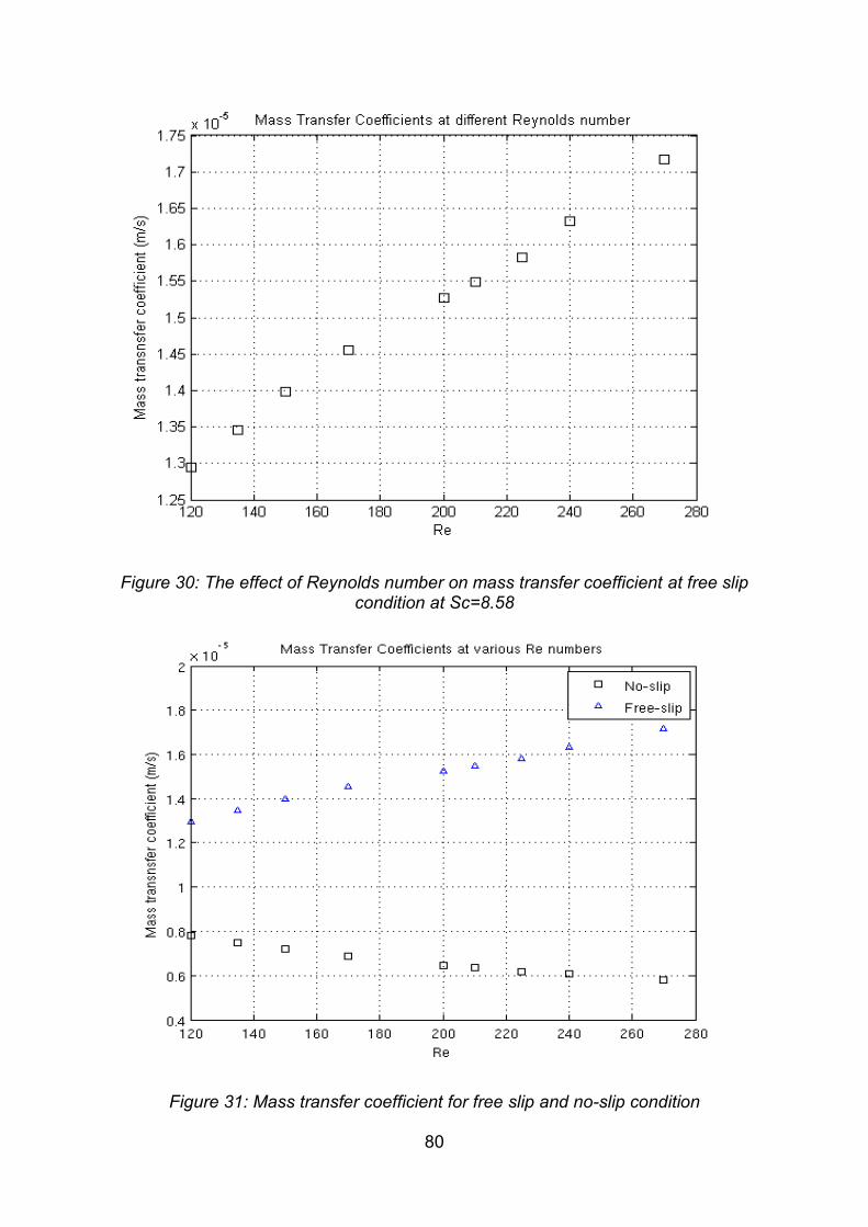
80
Figure 30: The effect of Reynolds number on mass transfer coefficient at free slip condition at Sc=8.58
Figure 31: Mass transfer coefficient for free slip and no-slip condition

81
Figure 32 illustrates the spherical symmetry concentration contours at Re = 30,
where the concentration of diffusing species decreases from the bubble surface to
bulk fluid. At this stage, the mass transfer is principally controlled by diffusion.
When the Re is increased, the concentration contours in front of the bubble decrease
in thickness and no symmetry is observed (Figure 33). The mass transfer mechanism
changes from diffusion to advection (bulk fluid diffusion) especially around the rear of
the bubble. In the case of no slip condition where there is separation of flow, mass
transfer occurs. Due to the recirculation (concentration wake), the fluid approaching
this region from the inlet has a certain concentration. Generally, the mass transfer
elements in the bulk fluid flow move around the rear of the bubble. This movement
causes the concentration in this region to increase and with continuous bulk liquid
movement, the fluid elements are transported away with fluid flow.
This advection movement explains the long concentration tail as seen in Figure 33. It
is important to note that in real turbulent reactors; the rate of mixing increases
causing no formation of tails.
Figure 32 : Nitrogen Concentration fields around bubble at Re=30 and Sc=8.58

82
Figure 33: Concentration contours around bubble at Re=270 and Sc=8.58
7.2.2. The Influence of Schmidt number on kla
The mass transfer coefficient is directly proportional to the mass diffusivity (Schmidt
number) as in Equation 6. As the diffusivity increases, the average mass transfer
coefficient also increases; this expected trend is seen in Figure 34. Li et al., (2003)
and Paschedag et al., (2005) also showed Sc has an effect on kla.
Figure 34: The effect of Schmidt number on mass transfer coefficient

83
7.3. Summary of Investigations The boundary layer condition specified on the bubble surface is very important
because it affects the velocity and concentration boundary layer. The velocity and
concentration boundary layer in turn affects the mass boundary layer thickness. The
mass boundary layer thickness and the mass diffusivity are used to calculate the
average mass transfer coefficient.
The average mass transfer coefficient increases with increasing Reynolds number as
the mass boundary layer thickness decreases for the free slip boundary condition.
This is expected, since there is no recirculation wake at the rear of the bubble and
these parameters are inversely proportional according to the film theory.
The same expected outcome is observed as the Schmidt number increases, the
mass boundary layer thickness also decreases and average mass transfer coefficient
increases. Therefore, as investigated, the Re and Sc numbers have an effect on the
mass boundary layer thickness and average mass transfer coefficients.
7.4. Mass Transfer Coefficients and BCM Section 7.2 shows that the estimated mass transfer coefficients are influenced by the
velocity field vectors and mass boundary layers thickness around the bubble. In
Figure 31, the simulated CFD results for free slip condition show the mass transfer
coefficient increasing as the Reynolds number increases. This is the expected trend
for the film theory; where mass transfer coefficients increase as Reynolds number
increases.
The simulated CFD results obtained are coherent with literature predictions and can
therefore be used to extend the BCM application to integrate mass transfer. The
mass transfer application to the BCM can be achieved by developing a general
algebraic function which directly estimates the mass transfer coefficient as a function
of Re and Sc numbers. Three different methods are investigated to determine if the
mass transfer coefficients can be estimated as a function of Re and Sc numbers.

84
7.4.1. Method 1 - Sherwood Number The Reynolds number and Sherwood number have an integral part to play when
estimating mass transfer coefficients. Several correlations as seen in Table 2
estimate mass transfer coefficient in the form of the Sherwood number. The mass
transfer coefficients values from the simulated CFD results are used to calculate
Sherwood number using Equation 9 and are illustrated in Figure 35. The observed
result is expected: since the mass transfer coefficient increase with Reynolds number
so does the Sherwood number.
Figure 35: Sherwood Number versus Reynolds number from simulated CFD Results
A curve fitting approach not found in literature is used to determine which algebraic
function suits the Sherwood in terms of Reynolds number. The results show that the
best fitting types were the Linear Polynomial and Power models with R2 of 0.9959
and 0.9939 respectively. Equations 50 and 51 below describe the models with the
Sherwood as a function of Reynolds number.

85
The simulated CFD results are used as a point of reference to determine which
model is most adapted to estimate mass transfer coefficients. The simulated CFD
results are then compared to linear polynomial and power functions models and
demonstrated in Figure 36. The polynomial function gives closer estimates to the
simulated CFD results, thereby being the best option out of the two models.
Therefore using Equation 50, the mass transfer coefficient can be estimated for a
system by simply inserting the Reynolds number.
Figure 36: Comparison of Mass transfer coefficients between CFD, Linear Polynomial
and Power models
7.4.2. Method 2 – Concentration Boundary Layer (Film Theory) The mass boundary layer thickness is greatly influenced by the Reynolds number as
described in Section 7.1.3. The outcome being that the mass boundary layer
thickness decreases with increasing Reynolds number as expected from film theory.
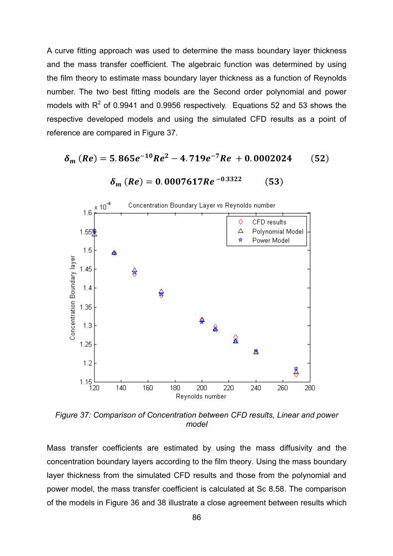
86
A curve fitting approach was used to determine the mass boundary layer thickness
and the mass transfer coefficient. The algebraic function was determined by using
the film theory to estimate mass boundary layer thickness as a function of Reynolds
number. The two best fitting models are the Second order polynomial and power
models with R2 of 0.9941 and 0.9956 respectively. Equations 52 and 53 shows the
respective developed models and using the simulated CFD results as a point of
reference are compared in Figure 37.
Figure 37: Comparison of Concentration between CFD results, Linear and power
model
Mass transfer coefficients are estimated by using the mass diffusivity and the
concentration boundary layers according to the film theory. Using the mass boundary
layer thickness from the simulated CFD results and those from the polynomial and
power model, the mass transfer coefficient is calculated at Sc 8.58. The comparison
of the models in Figure 36 and 38 illustrate a close agreement between results which

87
shows that different methods of correlating data yield approximately the same results.
These algebraic forms of estimating the mass transfer coefficient from the
concentration boundary layers as function of Reynolds number are good enough.
This method has an advantage because it not only gives the mass transfer coefficient
but also the mass boundary layer thickness around the bubble.
Figure 38: Comparison of Mass transfer coefficients between CFD, Linear Polynomial
and Power models
7.4.3. Method 3 – Velocity and Concentration Boundary Layer The film theory has been discussed in Section 2.1.1 and the simulated CFD results
showed the expected trend. However, the boundary layer theory described in Section
2.1.2 predicts the mass transfer coefficient with dependence on diffusivity. This
dependence is shown in Equation 14 which calculates the mass boundary layer
thickness but requires the momentum boundary layer thickness as developed in
Equation 13 (Dutta, 2007; Benitez, 2009). Figure 39 shows the estimated mass
transfer coefficients from the boundary layer theory and the expected outcome is
observed.

88
Figure 39: Estimated mass transfer coefficients from the boundary layer theory
A curve fitting approach was used to determine an algebraic function for estimating
mass transfer coefficient as a function of Re. The second order polynomial and
power model were the best fits for the velocity boundary layer with R2 of 0.9987 and
1 respectively. The developed Equations 54 and 55 were used to calculate mass
boundary thickness with Sc 8.58 as Equation 13 requires. There are no simulated
results to compare models; therefore a correlation developed by Benitez (2009) was
used as a point of reference. The comparison is shown in Figure 40 where the power
model and results from Benitez (2009) are in very good agreement for the
momentum boundary layer thickness and mass transfer coefficients.
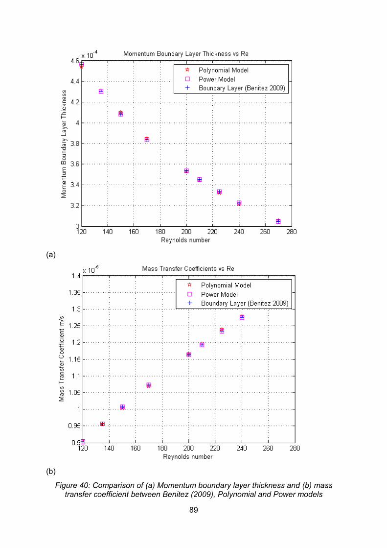
89
(a)
(b)
Figure 40: Comparison of (a) Momentum boundary layer thickness and (b) mass transfer coefficient between Benitez (2009), Polynomial and Power models

90
The same second order polynomial and power models gave good fits for the mass
boundary layer thickness with R2 of 0.9987 and 1 respectively. Equations 56 and 57
were directly used to calculate mass transfer coefficients using the film theory.
(a)

91
(b)
Figure 41: Comparison of (a) Momentum boundary layer thickness and (b) mass transfer coefficient between Polynomial and Power models
Figure 41 shows the good agreement between the estimated mass boundary layer
thickness and mass transfer coefficients from the velocity and concentration models.
7.4.4. Method Comparison
A model is most reliable if the R2 is at or closer to one and describes how accurate
the model fits the data. Looking at Table 6 below, the Polynomial velocity and
concentration boundary layer theory are the best models to use. However, it is
important to note that there are other factors considered when choosing the best
model. These factors include the validity and the effectiveness of the model.
Table 6: R2 Model Comparison
Model R2 Polynomial Sherwood 0.9959
Power Sherwood 0.9939 Polynomial Concentration BL 0.9941

92
Power Concentration BL 0.9956 Polynomial Velocity BL Theory 1
Power Velocity BL Theory 0.9987 Polynomial Concentration BL Theory 1
Power Concentration BL Theory 0.9987
Firstly, the validity of the model deals with the type of model, in this case polynomials
and power functions models. A power function also called a monomial function
models data that represents a proportional relationship increasing at a specific rate.
As shown above, all the power functions correspond to a direct or indirect variation
as the Reynolds number increasing.
A polynomial function is a sum of several monomial functions and is used when data
fluctuates but does not give details about the model, it only finding points that go near
data points. Therefore, preference is given to the power function models instead of
the polynomial models to estimate mass transfer coefficients.
Secondly, the effectiveness of the different models is compared to the simulated CFD
results and correlations. The estimates of the mass transfer coefficients from the
Sherwood number and Concentration boundary layer methods are very similar to the
CFD simulated results.
In conclusion, the estimates from the polynomial velocity and concentration boundary
layer theory give the best fit with R2 values of 1. However, polynomials are not the
desired models for this case study because it just fits the data points with no
additional details. This means all the polynomial functions used are scrapped and not
reliable for this project.
Looking now at only how the power functions models; the Sherwood and
concentration boundary layer gave the closest estimates to the CFD simulated
results with R2 of 0.9939 and 0.9956 respectively. Therefore, the chosen model to
predict mass transfer coefficients using the Reynolds and Schmidt number with an
elapsed time of 0.0409s is the concentration boundary layer power function
developed from the film theory in Equation 53 and rearranged in Equation 58 below.

93
7.4.5. Summary Firstly, the estimated mass transfer coefficients from the simulation and the
concentration boundary layer power function model show the expected trend with
increasing Reynolds number. As the Reynolds number increases, the mass transfer
coefficient also increases as in the film theory. The good agreement of the simulated
CFD and developed model shows that indeed, the mass transfer model can be
added to the BCM applications. Therefore, the mass transfer extension to the BCM
generates a general approach to determining the mass transfer coefficients than
using the various correlations in literature.
Secondly, inputs of Reynolds number and Schmidt number are required to estimate
the mass transfer coefficient. Unlike other models or correlations where gas hold-up
and superficial gas velocity calculations and so on are required before estimating the
mass transfer coefficient. An example of gas hold-up and mass transfer correlations
are shown in Dudley, 1995. Therefore, mass transfer extension to the BCM simply
requires only two input parameters and eliminates the time consuming calculations.
More so, from the developed model, the mass boundary layer thickness and mass
transfer coefficients for a nitrogen-water system are calculated. This indicates that,
with the BCM, an in-depth understanding and research can be achieved by analysing
the velocity pattern, concentration boundary layer formation, mass boundary layer
thickness and the mass transfer coefficients.
Finally, the BCM extension which is the concentration power function so far
demonstrates to be better and faster modelling approach. However, there is a need
to compare the estimated mass transfer coefficients against experimental data in
literature.

94
Chapter 8 Model Validation
8. Model Validation Model validation is essential because it gives credibility to the developed mass
transfer application to the BCM. The present study investigated the prediction of
average mass transfer coefficients in Bubble Column reactors by integrating the
mass balance into the BCM.
The simulated CFD results, BCM extension model and experimental data as
indicated in Table 2 are compared in Figure 42 below. The correlations in Table 2
have different geometries and experimental conditions such as solid spheres,
bubbles in liquid, drops, creeping regime just to name a few whereas the BCM
approach being a fundamental study simulates a single bubble in flowing liquid.
Figure 42: Model validation against experimental data

95
The following comments can be made when comparing the model with
experimentally determined correlations obtained from literature;
The literature correlations, CFD simulated results and the BCM extension
show the expected trend; as the Reynolds number increases, the mass
transfer coefficient also increases.
The mass transfer coefficients obtained from the BCM extension in Equation
58 are in good agreement to those obtained by Clift et al. (1978). This
illustrates how accurate the mass transfer extension to the BCM approach is
and can suitably be used to estimate the mass transfer coefficient for any
geometry or system.
The mass transfer coefficients values deduced from the Frössling (1938) and
Ranz and Marshal (1952) are also quite close to the BCM extension because
of the similar conditions used.
The correlations not in agreement with the BCM extension can be justified by
how mass transfer is sensitive to the choice of system, material properties,
operating conditions and equipment type. These parameters or factors have
an impact on the mass transfer coefficient. In addition, the different conditions
and geometry used in Table 2 like for example, single solid spheres, spherical
particles in fluid, rigid bubble surface just to name a few also affect the mass
transfer rate. Therefore, reproducing predictions or estimates of the mass
transfer coefficients as in the correlations is quite challenging.
Important to remember that the BCM Extension assumed the bubble size did
not change as fluid flows over the surface.
However, the BCM extension relies on the Reynolds number and is therefore only
valid for a limited range of applications. More so, chemical reactions were not
considered in the BCM development; thereby also limiting its applicability. On the
other hand, one way of improving its accuracy is to use the critical angle in Equation
48 for averaging of the mass boundary layer thickness.
96
Chapter 9 Conclusions
9. Conclusions
Numerous CFD models apart from the commonly used Euler-Euler, Euler-Lagrange
models have been developed to predict mass transfer coefficients. These
computationally expensive models are quite unique and depend on the operating
system.
In this case study, the CFD simulation results show varying mass boundary layer
thickness around a single spherical bubble in homogeneous nitrogen-water flow
regime. These mass boundary layer thicknesses were averaged using an integral
method to get a uniform mass boundary layer thickness around bubble. The mass
diffusivity and uniform mass boundary layer thickness are used to obtain the average
mass transfer coefficient.
The influence of the Reynolds and Schmidt numbers on mass boundary layer
thickness and average mass transfer coefficients from the CFD results was
investigated. It was shown that with increasing Re and Sc numbers, the mass
boundary layer thickness decreases and while the mass transfer coefficients
increase. As expected, simulation results indicate that to obtain high rates of mass
transfer, bubble column reactors should be operated at high Reynolds and Schmidt
numbers.
The BCM in its current approach only gives the velocity field vectors around a single
bubble. A general approach for estimating the average mass transfer coefficient is
required which is fundamentally based and not specific to equipment or operating
condition as compared to the numerous correlations.
The data from the simulated results were integrated to the BCM to develop an
algebraic function for estimating the mass transfer coefficient in bubble columns.
Three different methods were investigated to estimate the mass transfer coefficient
namely the Sherwood, Concentration boundary layer and the boundary layer theory.
The concentration boundary layer power function model was the best model which
gives the mass boundary layer thickness and the mass transfer coefficients.

97
The simulated results showed a close agreement when compared to literature
published correlations within a range of 120<Re<280. More so, a speed test of
0.0409s, confirms that the BCM mass transfer extension approach is a faster method
developed for generating the mass transfer coefficients. However, the range of
applicability is limited in terms of the Reynolds number and which needs to be fully
extended for major progress.
Therefore, a two dimensional semi-analytical fundamental model, the Bubble Cell
Model, requires the Reynolds and Schmidt numbers to generate the steady-state
velocity vector fields and estimate the gas-liquid mass transfer rate from spherical
bubbles in bubble columns in a homogeneous regime.
The BCM mass transfer extension calculates the mass transfer coefficient which
gives information on mass transfer rates in a non-reactive system. With the aid of the
population balance model, the bubble size effect can be established and an entire
Bubble Column simulated. Many systems in industry are reactive in one way or the
other. BCM applications are set to increase upon validation with chemical balance in
industry
Chapter 10 Recommendations
10. Recommendations The mass transfer addition to the BCM approach needs the Reynolds number to
estimate the average mass transfer coefficient. In this study, a limited range of
Reynolds number was used and therefore makes the approach only valid for limited
applications in homogeneous regimes. Furthermore, chemical reactions were not
considered in the BCM development; thus limiting its applicability. The BCM
approach will make strong progress in its development if applied in turbulent regime
with chemical reactions.

98
Chapter 11 References and Appendices
11. References
[Online]. Available: http://www.fluent.com.
[Online]. Available: http://www.flowlab.fluent.com.
[Online]. Available: http://www.cfdrc.com.
[Online]. Available: http://www.cd-adapco.com.
[Online]. Available: http://www.software.aeat.com/cfx.
[Online]. Available: http://www.macs.hw.ac.uk/~ms713/lecture_1.pdf .
Akhtar, A. 2006. Two-fluid Eulerian simulation of bubble column reactors with distributors. Journal of chemical engineering of japan. 39(8):831-841.
Akita, K. 1973. Gas Hold-up and Volumetric Mass Transfer coefficient in Bubble
Akita, K. 1974. Bubble size, interfacial area, and liquid-phase mass transfer coefficient in bubble columns. Industrial engineering chemistry process design and development. 13(1):84.
Alvarez, E. and others. 2000. Model based in neural networks for the prediction of the mass transfer coefficients in bubble columns. Study in Newtonian and non-Newtonian fluids. International communications in heat and mass transfer. 27(1):93-98.
Alvarez‐Cuenca, M. & Nerenberg, M. 1981. Oxygen mass transfer in bubble columns working at large gas and liquid flow rates. AIChE journal. 27(1):66-73.
Anil, M. 2007. CFD modeling of three-phase bubble column: 1. study of flow pattern. Chemical and biochemical engineering quarterly. 21(3):197.
Apte, S. and others. 2004. Large-eddy simulation of reacting turbulent flows in complex geometries. Comput.phys. 197:215-240.
Aroonwilas, A. and others. 2003. Mathematical modelling of mass-transfer and hydrodynamics in CO2 absorbers packed with structured packings. Chemical engineering science. 58(17):4037-4053.
Asgharpour, M. 2010. Effect of surface contaminants on oxygen transfer in bubble column reactors. Biochemical engineering journal. 49(3):351.
Baehr, H.D. & Karl, S. 2006. Heat and Mass Transfer. 2nd ed. Springer.

99
Baehr, H. & Stephan, K. 1998. Heat and mass transfer . Berlin and New York: Springer-Verlag.
Baker, T.J. 2005. Mesh generation: Art or science. Progress in aerospace sciences. 41(1):29-63.
Basmadjian, D. 2004. Mass Transfer: Principles And Applications. London: CRC Press.
Bauer, M. & Eigenberger, G. 2001. Multiscale modeling of hydrodynamics, mass transfer and reaction in bubble column reactors. Chemical engineering science. 56(3):1067-1074.
Bech, K. 2005. Dynamic simulation of a 2D bubble column. Chemical engineering science. 60(19):5294.
Becker, S., Sokolichin, A. & Eigenberger, G. 1994. Gas—liquid flow in bubble columns and loop reactors: Part II. Comparison of detailed experiments and flow simulations. Chemical engineering science. 49(24):5747-5762.
Becker, S. 1999. Dynamic flow behaviour in bubble columns. Chemical engineering science. 54(21):4929.
Benitez, J. 2009. Principles and modern applications of mass transfer operations.
Bergman, T.L. and others. 2011. Fundamentals of heat and mass transfer. Wiley.
Bhaga, D., Weber, M. E., 1981. Bubbles in viscous liquids: shapes, wakes and velocities. Journal of Fluid Mechanics 105, 301{318. ix, 21, 23
Bi, H. 2004. Multiscale analysis and modeling of multiphase chemical reactors. Advanced powder technology. 15(6):607.
Bin, A.K., Duczmal, B. & Machniewski, P. 2001. Hydrodynamics and ozone mass transfer in a tall bubble column. Chemical engineering science. 56(21-22):6233-6240.
Bird, R.B., Stewart, W.E. & Lightfoot , E.N. 1960. Transport Phenomena. New york: Wiley.
Botton, R., Cosserat, D. & Charpentier, J.C. 1980. Mass transfer in bubble columns operating at high gas throughputs. The chemical engineering journal. 20(2):87-94.
Bouaifi, M. and others. 2001. A comparative study of gas hold-up, bubble size, interfacial area and mass transfer coefficients in stirred gas–liquid reactors and bubble columns. Chemical engineering and processing: Process intensification. 40(2):97-111.

100
Bowman, C. and others. 1961. Mass transfer from fluid and solid spheres at low Reynolds numbers. The Canadian journal of chemical engineering. 39(1):9-13.
Brain, P.L.T. & Hales, H.B. 1969. Effects of transpiration and changing diameter on heat and mass transfer to spheres. A.I.ch.E. J. 15:419.
Brennen, C.E. 2005. Fundamentals of multiphase flow. Cambridge University Press. New York
Bukur, D.B. & Daly, J.G. 1987. Gas hold-up in bubble columns for Fischer-Tropsch synthesis. Chemical engineering science. 42(12):2967-2969.
Burnett, D.S. 1987. Finite Element Analysis - From Concepts to Application.. Reading: Addison-Wesley Publishing Company.
Buwa, V.V., Deo, D.S. & Ranade, V.V. 2006. Eulerian–Lagrangrian simulations of unsteady gas–liquid flows in bubble columns. International journal of multiphase flow. 32(7):864-885.
Buwa, V.V. & Ranade, V.V. 2004. Characterization of dynamics of gas–liquid flows in rectangular bubble columns. AIChE journal. 50(10):2394-2407.
Cachaza, E. 2009. Simultaneous Computational Fluid Dynamics (CFD) simulation of the hydrodynamics and mass transfer in a partially aerated bubble column. Industrial engineering chemistry research. 48(18):8685.
Carra, S. & Morbidelli, M. 1987. Gas–liquid reactors. Chemical reaction and reactor engineering, marcel dekker, New York. :545-666.
Chang, H. 1989. Measurement of Kla by a gassing-in method with oxygen-enriched air. Biotechnology and bioengineering. 34(9):1147.
Chrysikopoulos, C.V. and others. 2003. Mass transfer coefficient and concentration boundary layer thickness for a dissolving NAPL pool in porous media. Journal of hazardous materials. 97(1-3):245-255.
Clarke, K.G. & Correia, L.D.C. 2008. Oxygen transfer in hydrocarbon–aqueous dispersions and its applicability to alkane bioprocesses: A review. Biochemical engineering journal. 39(3):405-429.
Clarke, K.G. and others. 2006. Enhancement and repression of the volumetric oxygen transfer coefficient through hydrocarbon addition and its influence on oxygen transfer rate in stirred tank bioreactors. Biochemical engineering journal. 28(3):237-242.
Clift, R., Grace J.R & Weber M.E 1978. Bubbles, drops and particles. New York: Academic Press.
101
Coetzee, W., Coetzee, R. & Rawatlal, R. 2009. A statistical approach to computational fluid dynamics in predicting bubble columns. International Symposium on Business and Industrial Statistics.
Coetzee, W., Coetzer, R. J. L., and Rawatlal, R. (2010). An analysis of response surface strategies in developing statistical models for application in bubble column modelling. submitted to: Computers & Chemical Engineering.
Coetzee, W., Coetzer, R.L.J. & Rawatlal, R. 2012a. Response surface strategies in constructing statistical bubble flow models for the development of a novel bubble column simulation approach. Computers & chemical engineering. 36:22-34.
Coetzee, W., Coetzer, R. & Rawatlal, R. 2012b. Development of a computationally efficient bubble column simulation approach by way of statistical bubble micro-flow modelling. Advances in fluid mechanics IX. 9:275.
Coetzee, W., Coetzer, R.L. & Rawatlal, R. 2012c. Semi analytical Bubble-Flow Models for the Development of a Novel Bubble-Column Simulator. Industrial & engineering chemistry research. 51(21):7398-7409.
Correia, L.D.C., Aldrich, C. & Clarke, K.G. 2010. Interfacial gas–liquid transfer area in alkane–aqueous dispersions and its impact on the overall volumetric oxygen transfer coefficient. Biochemical engineering journal. 49(1):133-137.
Crumpton, P.I., Moinier, P. & Giles, M.B. 1997. An unstructured algorithm for high Reynolds number flows on highly stretched meshes. Numerical methods in laminar and turbulent flow. :561–572.
Cussler, E.L. 2003. Diffusion: Mass Transfer in Fluid Systems. 2nd ed. Cambridge University Press.
Dani, A., Cockx, A. & Guiraud, P. 2006. Direct numerical simulation of mass transfer from spherical bubbles: the effect of interface contamination at low Reynolds numbers. International journal of chemical reactor engineering. 4(1).
Darmana, D. 2007. Detailed modelling of hydrodynamics, mass transfer and chemical reactions in a bubble column using a discrete bubble model: Chemisorption of CO2 into NaOH solution, numerical and experimental study. Chemical engineering science. 62(9):2556.
Darmana, D., Deen, N.G. & Kuipers, J.A.M. 2005. Detailed modeling of hydrodynamics, mass transfer and chemical reactions in a bubble column using a discrete bubble model. Chemical engineering science. 60(12):3383-3404.
Deckwer, W.D., Burckhart, R. & Zoll, G. 1974. Mixing and mass transfer in tall bubble columns. Chemical engineering science. 29(11):2177-2188.
Deckwer, W.D. 1992. Bubble column reactors. Chichester: .

102
Deckwer, W.-. 1983. APPLICABILITY OF AXIAL DISPERSION MODEL TO ANALYZE MASS TRANSFER MEASUREMENTS IN BUBBLE COLUMNS. AICHE journal. 29(6):915.
Deen, N.G., Solberg, T. & Hjertager, B.H. 2001. Large eddy simulation of the gas–liquid flow in a square cross-sectioned bubble column. Chemical engineering science. 56(21):6341-6349.
Degaleesan, S. 2001. Experimental study of gas‐induced liquid‐flow structures in bubble columns. AIChE journal. 47(9):1913.
Deindoerfer, F. & Humphrey, A. 1961. Mass transfer from individual gas bubbles. Industrial & engineering chemistry. 53(9):755-759.
Delnoij, E., Kuipers, J. & Van Swaaij, W. 1999. A three-dimensional CFD model for gas–liquid bubble columns. Chemical engineering science. 54(13):2217-2226.
Delnoij, E. and others. 1997. Dynamic simulation of dispersed gas-liquid two-phase flow using a discrete bubble model. Chemical engineering science. 52(9):1429-1458.
Delnoij, E. 1997. Dynamic simulation of gas-liquid two-phase flow: Effect of column aspect ratio on the flow structure. Chemical engineering science. 52(21):3759.
Delnoij, E. 1999. A three-dimensional CFD model for gas-liquid bubble columns. Chemical engineering science. 54(13):2217.
Dhaouadi, H. and others. 2008. Gas–liquid mass transfer in bubble column reactor: Analytical solution and experimental confirmation. Chemical engineering and processing: Process intensification. 47(4):548-556.
Dudley, J. 1995. Mass transfer in bubble columns: a comparison of correlations. Water research. 29(4):1129-1138. .
Dutta, B.K. 2007. Principles of mass transfer and separation processes. Prentice-Hall of India.
Ekambara, K. 2003. CFD simulation of mixing and dispersion in bubble columns. Chemical engineering research and design. 81(8):987.
Ekambara, K. 2005. CFD simulations of bubble column reactors: 1D, 2D and 3D approach. Chemical engineering science. 60(23):6733.
Ekambara, K. 2010. CFD simulation of bubble column. Nuclear engineering and design. 240(5):963.
Ekambara, K. 2005. Computational fluid dynamics simulations in bubble-column reactors: Laminar and transition regimes. Industrial engineering chemistry research. 44(5):1413.

103
Ekambara, K. 2008. CFD simulation of bubble column reactor using population balance. Industrial engineering chemistry research. 47(21):8505.
Ellenberger, J. 2002. Improving mass transfer in gas-liquid dispersions by vibration excitement. Chemical engineering science. 57(22):4809.
Erkey, C. 1990. Correlation for predicting diffusion coefficients in alkanes. The Canadian journal of chemical engineering. 68(4):661.
Eymard, R., Gallouet, T. & Herbin, R. Eds. 2006. Finite Volume Methods. 7th ed. Marseille: Ciarlet, P.G. and Lions eds,.
Ferrel, R.T. & Himmelblau, D.M. 1967. Diffusion coefficients of nitrogen and oxygen in water. Journal of chemical and engineering data. 12(1):111-115.
Fleischer, C., Becker, S. & Eigenberger, G. 1996. Detailed modeling of the chemisorption of CO2 into NaOH in a bubble column. Chemical engineering science. 51(10):1715-1724.
Friedlander, S. 1957. Mass and heat transfer to single spheres and cylinders at low Reynolds numbers. AIChE journal. 3(1):43-48.
Frössling, N. 1938. Uber die Verdunstung fallender Tropfen. Gerlands beitr. geophys. 52:170.
Gandhi, A. 2009. Development of unified correlations for volumetric mass-transfer coefficient and effective interfacial area in bubble column reactors for various gas-liquid systems using support vector regression. Industrial engineering chemistry research. 48(9):4216.
Garcia, M.J., Boulanger, P. & Giraldo, S. 2008. CFD based wing shape optimization through gradient-based method. EngOpt 2008-International Conference on Engineering Optimization. 01.
Garcia-Ochoa, F. 2005. Prediction of gas‐liquid mass transfer coefficient in sparged stirred tank bioreactors. Biotechnology and bioengineering. 92(6):761.
Garcia-Ochoa, F. & Gomez, E. 2004. Theoretical prediction of gas–liquid mass transfer coefficient, specific area and hold-up in sparged stirred tanks. Chemical engineering science. 59(12):2489-2501.
Garner, F.H. & Keey, R.B. 1958. Mass Transfer from Single Solid Spheres - I. Transfer at Low Reynolds numbers. Chem. eng. sci. 9:119.
Garner, F.H. & Keey, R.B. 1959. Mass Transfer from Single Solid Spheres - II. Transfer in free Convection. Chem. eng.sci. 9:218.
Gartling, D.K. 2002. Applied CFD Techniques: An Introduction based on Finite Element methods. by R. Löhner, John Wiley Sons, Chichester 2001, Number of

104
pages: 376. ISBN 0‐471‐49843‐2. Price: $95.00. International journal for numerical methods in fluids. 39(1):97.
Gestrich, W., Esenwein, H. & Krauss, W. 1976. Der flüssigkeitsseitige Stoffübergangskoeffizient in Blasenschichten. Chemie ingenieur technik. 48(5):399. [Online]. Available: http://dx.doi.org/10.1002/cite.330480509.
Gogate, P.R. & Pandit, A.B. 1999. Survey of measurement techniques for gas–liquid mass transfer coefficient in bioreactors. Biochemical engineering journal. 4(1):7-15.
Gómez-Díaz, D. & Navaza, J.M. 2005. Gas/liquid mass transfer in carbon dioxide–alkanes mixtures. Chemical engineering journal. 114(1-3):131-137.
Gómez-Díaz, D. and others. 2009. Oxygen mass transfer to emulsions in a bubble column contactor. Chemical engineering journal. 152(2-3):354-360.
Gorji, M. 2006. A three dimensional CFD modeling of hydrodynamics and mass transfer in a gas-liquid impeller stirred tank reactor.
Gray, M. 1993. Liquid-side mass transfer coefficients for liquids and slurries in a rotating drum. Chemical engineering science. 48(19):3442.
Grund, G., Schumpe, A. & Deckwer, W.-. 1992. Gas-Liquid mass transfer in a bubble column with organic liquids. Chemical engineering science. 47(13-14):3509-3516.
Hadamard, J. S. (1911). "Mouvement permanent lent d'une sphère liquide et visqueuse dans un liquide visqueux". CR Acad. Sci. 152: 1735. Rybczynski, W.
Hamborg, E.S. & Versteeg, G.F. 2012. Absorption and desorption mass transfer rates in chemically enhanced reactive systems. Part I: Chemical enhancement factors. Chemical engineering journal. 198–199(0):555-560.
Hammer, H. and others. 1984. New Sub functions on Hydrodynamics, Heat and Mass Transfer for Gas/Liquid and Gas/Liquid/Solid Chemical and Biochemical Reactors. Front.chem.reac.eng. 464.
Han, L. 2007. Gas-liquid mass transfer in a high pressure bubble column reactor with different sparger designs. Chemical engineering science. 62(1):131.
Hasegawa, Y. & Kasagi, N. 2001. The effect of Schmidt number on air-water interface mass transfer. Proceeding of the 4th international conference on multiphase flow, New Orleans.
Hashemi, S. 2009. Gas-liquid mass transfer in a slurry bubble column operated at gas hydrate forming conditions. Chemical engineering science. 64(16):3709.

105
Haut, B. & Cartage, T. 2005. Mathematical modeling of gas–liquid mass transfer rate in bubble columns operated in the heterogeneous regime. Chemical engineering science. 60(22):5937-5944.
Hikita, H. and others. 1980. Gas hold-up in bubble columns. The chemical engineering journal. 20(1):59-67.
Hikita, H. and others. 1981. The volumetric liquid-phase mass transfer coefficient in bubble columns. The chemical engineering journal. 22(1):61-69.
Hua, J. and Lou, J. (2007). Numerical simulation of bubble rising in viscous liquid. Journal of Computational Physics, 222:769{795.
Hughmark, G.A. 1967. Holdup and mass transfer in bubble columns. 6(2):218-220.
Hung, T. and others. 2007. An innovative improvement of engineering learning system using computational fluid dynamics concept. Computers & education. 48(1):44-58.
Incropera, F.P. and others 2011. Fundamentals of heat and mass transfer. Wiley
Irani, M. & Khodagholi, M.A. 2011. INVESTIGATION OF BUBBLE COLUMN HYDRODYNAMICS USING CFD SIMULATION (2D AND 3D) AND EXPERIMENTAL VALIDATION. Petroleum & coal. 53(2):146-158.
Jajuee, B. 2006. Application of surface-renewal-stretch model for interface mass transfer. Chemical engineering science. 61(12):3917.
Jin, H. 2004. Experimental study of oxygen mass transfer coefficient in bubble column with high temperature and high pressure. Chemical engineering technology. 27(12):1267.
Jorge, M.T.V., Orvalho, S.P. & Sebastiao, S.A. 2002. Alche journal. 48(6):1145-1154.
Joshi, J.B. 2001. Computational flow modelling and design of bubble column reactors. Chemical engineering science. 56(21):5893.
Joshi, J. 2003. Computational fluid dynamics for designing process equipment: Expectations, current status, and path forward. Industrial engineering chemistry research. 42(6):1115.
Kang, Y. 1999. Diagnosis of bubble distribution and mass transfer in pressurized bubble columns with viscous liquid medium. Chemical engineering science. 54(21):4887.
Kantarci, N., Borak, F. & Ulgen, K.O. 2005. Bubble column reactors. Process biochemistry. 40(7):2263-2283.

106
Kawase, Y., Halard, B. & Moo-Young, M. 1987. Theoretical prediction of volumetric mass transfer coefficients in bubble columns for Newtonian and non-Newtonian fluids. Chemical engineering science. 42(7):1609-1617.
Kawase, Y. & Moo-Young, M. 1987. Theoretical prediction of gas hold-up in bubble columns with Newtonian and non-Newtonian fluids. Industrial & engineering chemistry research. 26(5):933-937.
Kawase, Y., Umeno, S. & Kumagai, T. 1992. The prediction of gas hold-up in bubble column reactors: Newtonian and non-Newtonian fluids. The chemical engineering journal. 50(1):1-7.
Kayode Coker, A. 2001. Modelling of Chemical Kinetics and Reactor Design. Boston: Gulf Publ.,.
Kelly, W. 2008. Using computational fluid dynamics to characterize and improve bioreactor performance. Biotechnology and applied biochemistry. 49(3):225.
Kenig, E.Y. 2007. Advanced modeling of reactive separation units with structured packings. Chemical product and process modeling. 2(1).
Koeltzsch, K. 2000. The height dependence of the turbulent Schmidt number within the boundary layer. Atmospheric environment. 34(7):1147-1151.
Kojima, H., Sawai, J. & Suzuki, H. 1997. Effect of pressure on volumetric mass transfer coefficient and gas holdup in bubble column. Chemical engineering science. 52(21-22):4111-4116.
Krishna, R. 1994. Strategies for multiphase reactor selection. Chemical engineering science. 49(24):4029.
Krishna, R. 2002. Improving gas-liquid mass transfer in bubble columns by applying low-frequency vibrations. Chemical engineering technology. 25(2):159.
Krishna, R. 2003. Mass transfer in bubble columns. Catalysis today. 79:67.
Krishna, R. & Ellenberger, J. 2002. Improving gas–liquid contacting in bubble columns by vibration excitement. International journal of multiphase flow. 28(7):1223-1234.
Krishna, R. & Sie, S.T. 2000. Design and scale-up of the Fischer–Tropsch bubble column slurry reactor. Fuel processing technology. 64(1–3):73-105.
Kulkarni, A.A. 2007. On the development of flow pattern in a bubble column reactor: Experiments and CFD. Chemical engineering science. 62(4):1049.
Kulkarni, A.A. & Joshi, J.B. 2004. Simultaneous measurement of flow pattern and mass transfer coefficient in bubble columns. Chemical engineering science. 59(2):271-281.

107
Kumar, A. 2009. CFD Modeling of Gas-Liquid-Solid Fluidized Bed. B.Tech. NIT,Rourkela,.
Kumar, S., Srinivasulu, N., & Khanna, A. CFD Simulations to Validate Two & Three Phase Up-flow in Bubble Columns.
Kundu, A. 2003. Mass transfer characteristics in gas-liquid-liquid system. The canadian journal of chemical engineering. 81(3):640.
Kuzmin, D. & Turek, S. 2000. Efficient numerical techniques for flow simulation in bubble column reactors. Univ. Dortmund, Fachbereich Mathematik.
Löhner, R. 2001. Applied CFD Techniques: An Introduction based on Finite Element methods. Chichester: John-Wiley and Sons Ltd.
Laari, A. 1997. Gas-liquid mass transfer in bubble columns with a T-junction nozzle for gas dispersion. Chemical engineering technology. 20(8):550.
Laın, S. 2002. Modelling hydrodynamics and turbulence in a bubble column using the Euler–Lagrange procedure. International journal of multiphase flow. 28(8):1381.
Lau, R. and others. 2004. Gas-liquid mass transfer in high-pressure bubble columns. Industrial & engineering chemistry research. 43(5):1302-1311.
Law, D. 2006. Numerical simulations of gas-liquid flow dynamics in bubble columns. Fed.
Lee, K. D. ,Loellbach, J. M and . Kim. M. S 1991. "Adaptive control of grid quality for computational fluid dynamics", Journal of Aircraft, Vol. 28, No. 10, pp. 664-669. doi: 10.2514/3.46080
Lemoine, R. and others. 2008. An algorithm for predicting the hydrodynamic and mass transfer parameters in bubble column and slurry bubble column reactors. Fuel processing technology. 89(4):322-343.
Levenspiel, O. 1988. Chemical engineering's grand adventure. Chem. engng sci. 43:1427-1435.
Levenspiel, O. 1999. Chemical Reaction Engineering. Chichester: Wiley J.
Li, W.Z., Yan, Y.Y. & Smith, J.M. 2003. A numerical study of the interfacial transport characteristics outside spheroidal bubbles and solids. International journal of multiphase flow. 29(3):435-460.
Linton, M. & Sutherland, K. 1960. Transfer from a sphere into a fluid in laminar flow. Chemical engineering science. 12(3):214-229.
Liu, S.X., Peng, M. & Vane, L. 2004. CFD modeling of pervaporative mass transfer in the boundary layer. Chemical engineering science. 59(24):5853-5857.

108
Lochiel, A. & Calderbank, P. 1964. Mass transfer in the continuous phase around axisymmetric bodies of revolution. Chemical engineering science. 19(7):471-484.
Lu, S. and others. 2003. Measurement of the Bubble Parameters in Bubble Column by Conductivity Probe. Chemical reaction engineering and technology. 19(4):344-351.
Maalej, S. 2001. Influence of pressure on the hydrodynamics and mass transfer parameters of an agitated bubble reactor. Chemical engineering technology. 24(1):77.
MacCormack, R.W. & Baldwin, B.S. 1975. A numerical method for solving the Navier-Stokes equations with application to shock-boundary layer interactions. American institute of aeronautics and astronautics, aerospace sciences meeting, 13th, pasadena, calif., jan. 20-22, 1975, 9 p.
Maceiras, R., Santana, R. & Alves, S.S. 2007. Rise velocities and gas–liquid mass transfer of bubbles in organic solutions. Chemical engineering science. 62(23):6747-6753.
Madhavi, T. 2007. Studies on bubble dynamics with mass transfer. Chemical engineering journal. 128(2):95.
Mahajan, V. 2010. CFD analysis of hydrodynamics and mass transfer of a gas-liquid bubble column.
Mahesh, K. 2006. Large-eddy simulation of reacting turbulent flows in complex geometries. Journal of applied mechanics. 73(3):374.
Mangartz, K.H. 1981. Interpretation of Mass Transfer Measurements in Bubble Columns considering dispersion of both. Chemical engineering science. 36(6):1069.
Mangartz, K. 1980. Studies of the Gas Phase Dispersion in Bubble Column Reactors. Verfahrenstechnik. 14(1):40.
Maretto, C. & Krishna, R. 1999. Modelling of a bubble column slurry reactor for Fischer–Tropsch synthesis. Catalysis today. 52(2-3):279-289.
Margavey, R.H. and Bishop, R.L., “Transition ranges for three-dimensional wakes”, Can. J. Phys., 39, 1418-1422, 1961.
Mark M.Clark Ed. 2009. Transport Modelling for Environmental Engineers and Scientist. 2nd ed. United Kingdom: John Wiley & Sons,Inc.,.
Martín, M., Montes, F.J. & Galán, M.A. 2009a. Mass transfer from oscillating bubbles in bubble column reactors. Chemical engineering journal. 151(1-3):79-88.

109
Martín, M., Montes, F.J. & Galán, M.A. 2009b. Theoretical modelling of the effect of surface active species on the mass transfer rates in bubble column reactors. Chemical engineering journal. 155(1-2):272-284.
Mashelkar, R. & Sharma, M. 1970. Mass transfer in bubble and packed bubble columns. Transactions of the institution of chemical engineers. 48:T162-T162.
McCready, M.J. 2003. Principles and modern applications of mass transfer operations. By Jaime Benitez, Wiley, New York 2002, 499 pp., $89.95. AIChE journal. 49(1):288.
Medic, L. and others. 1989. Volumetric gas-liquid mass transfer coefficients in a rectangular bubble column with a rubber aeration pad. The chemical engineering journal. 41(3):B51-B54.
Merchuk, J.C. & Ben-Zvi(Yona), S. 1992. A novel approach to the correlation of mass transfer rates in bubble columns with non- Newtonian liquids. Chemical engineering science. 47(13-14):3517-3523.
Michaelides, E.E. 2006. Particles, Bubbles & Drops Thier Motion,Heat and Mass transfer. Singapore: World Scientific Publishing Co. Pte. Ltd.
Miyahara, T. 1997. Gas holdup, gas-liquid interfacial area and mass transfer coefficient in external-loop airlift bubble column containing low density particles. Journal of chemical engineering of japan. 30(5):958.
Mohapatra, D. & Rakh, K. 2007. CFD Modeling of Multi-phase Fluidized Bed. B. Tech. NIT.
Motarjemi, M. & Jameson, G. 1978. Mass transfer from very small bubbles—the optimum bubble size for aeration. Chemical engineering science. 33(11):1415-1423.
Mousavi, S.M. 2008. Experiments and CFD simulation of ferrous bio oxidation in a bubble column bioreactor. Computers chemical engineering. 32(8):1681.
Mudde, R. 1999. Two- and three-dimensional simulations of a bubble plume using a two-fluid model. Chemical engineering science. 54(21):5061.
Muller, F.L. & Davidson, J.F. 1992. On the contribution of small bubbles to mass transfer in bubble columns containing highly viscous liquids. Chemical engineering science. 47(13-14):3525-3532.
Nakamura, I., “Steady wake behind a sphere”, Phys. Fluids, 19(1), pp. 5-8, 1976.
Natarajan, R. and Acrivos, A., “The instability of the steady flow past spheres and disks”, J. Fluid Mech. 254, 323-344, 1993.

110
Ouyoung, P.K., Nam Chang, H. & Moo-Young, M. 1988. Determination of gas-liquid mass transfer coefficient in a bubble column by an eigenvalue method. Chemical engineering science. 43(4):821-827.
Oyevaar, M.H. and others. 1989. Interfacial areas and gas hold-ups in bubble columns and packed bubble columns at elevated pressures. Chemical engineering and processing: Process intensification. 26(1):1-14.
Öztürk, S. & Schumpe, A. 1987. The influence of suspended solids on oxygen transfer to organic liquids in a bubble column. Chemical engineering science. 42(7):1781-1785.
Pantankar, S. V. (1980). Numerical Heat Transfer and Fluid Flow. Taylor & Francis. Tomiyama, A., Celata, G. P., Hosokawa, S., and Yoshida, S. (2002). Terminal velocity of single bubbles in surface tension force dominant regime. International Journal of Multiphase Flow, 28:1497{1519.
Parasu Veera, U. & Joshi, J.B. 2000. Measurement of Gas Hold-up Profiles in Bubble Column by Gamma Ray Tomography: Effect of Liquid Phase Properties. Chemical engineering research and design. 78(3):425-434.
Paschedag, A., Piarah, W. & Kraume, M. 2005. Sensitivity study for the mass transfer at a single droplet. International journal of heat and mass transfer. 48(16):3402-3410.
Peraire, J., Morgan, K. & Peiro, J. 1989. Unstructured finite element mesh generation and adaptive procedures for CFD. AGARD FDP: specialist's meeting, Loen, Norway. DTIC Document.
Pfleger, D. & Becker, S. 2001. Modelling and simulation of the dynamic flow behaviour in a bubble column. Chemical engineering science. 56(4):1737-1747.
Pilhofer, T. 1978. Determination of Fluid Dynamic Parameters in bubble Column Design. ACS symposium series. (65):372.
Ponoth, S.S. & McLaughlin, J. 2000. Numerical simulation of mass transfer for bubbles in water. Chemical engineering science. 55(7):1237-1255.
Ranade, V.V. 2001. Computational flow modeling for chemical reactor engineering. Academic press.
Ranade, V.V. 2002. Computational Flow Modeling for Chemical Reactor Engineering.
Ranz, W.E. & Marshall, W.R. 1952. Evaporation from drops Part II. Chem.eng.prog. 48:173.
Rodemerck, U. & Seidel, A. 1991. Analysis of transient mass transfer measurements in bubble columns. Chemical engineering science. 46(3):908-912.
111
Rowe, P.N.C., K.T. & Lewis, J.B. 1965. Heat and Mass Transfer from a single sphere in an extensive flowing fluid. Trans. inst. chem. eng. 41:T14.
Sada, E. and others. 1975. Diffusivities of gases in binary mixtures of alcohols and water. The chemical engineering journal. 10(1):155-159.
Sada, E. 1986. Gas holdup and mass-transfer characteristics in a three-phase bubble column. Industrial engineering chemistry process design and development. 25(2):472.
Samareh, J.A. 2005. Geometry and grid/mesh generation issues for CFD and CSM shape optimization. Optimization and engineering. 6(1):21-32.
Sawant, S.B., Pangarkar, V.G. & Joshi, J.B. 1979. Gas hold-up and mass transfer characteristics of packed bubble columns. The chemical engineering journal. 18(1):143-149.
Schlichting, H. Boundary Layer Theory, McGraw-Hill, New York, 1968
Schlüter, S. 1995. Simulation of bubble column reactors with the BCR computer code. Chemical engineering and processing. 34(2):127.
Schumpe, A. & Deckwer, W.D. 2004. Organic liquids in a bubble column: holdups and mass transfer coefficients. AIChE journal. 33(9):1473-1480.
Seader, J.D., Henley, E.J. & Roper, D.K. Eds. 2010. Separation Process Principles. 3rd ed.: John Wiley and Sons.
Seader, J. & Henley, E. Separation Process Principles. 2006, Hoboken.
Seader, J. & Henley, E. 1998. Separation process principlesWiley. New york.
Seebauer, E.G. 1995. Estimating surface diffusion coefficients. Progress in surface science. 49(3):265.
Shah, Y.T. 1982. DESIGN PARAMETERS ESTIMATIONS FOR BUBBLE COLUMN REACTORS. AICHE journal. 28(3):353.
Shaikh, A. & Al-Dahhan, M. 2007. A Review on Flow Regime Transition in Bubble Columns. International journal of chemical reactor engineering. 5.
Sherwood, T.K., Pigford, R.L. & Wilke, C.R. 1975. Mass Transfer. New York: McGraw-Hill.
Shimizu, K. 2000. Phenomenological model for bubble column reactors: Prediction of gas hold-ups and volumetric mass transfer coefficients. Chemical engineering journal. 78(1):21.
Silva, E., Teixeira, S. & Lobarinhas, P. 2008. The influence of different grid approaches on a cardiovascular computational model, Proceeding of the 17th

112
IASTED I nternational Conference on Applied Simulation and Modelling 2008,9780889867482, Corfu, Greece, June 2008, ACTA Press,Calgary
Silva, E., Teixeira, S. & Lobarinhas, P. 2011. Computational Fluid Dynamics Simulations:an Approach to Evaluate Cardiovascular Dysfunction, Modelling Simulation and Optimization, Gregorio Romero Rey and Luisa Martinez Muneta (Ed.), ISBN: 978-953-307-048-3, InTech, Available from: http://www.intechopen.com/books/modelling-simulation-and optimization/computational-fluid-dynamicssimulations-an-approach-to-evaluate-cardiovascular-dysfunction.
Singh, M.K. & Majumder, S.K. 2011. Co-and counter-current mass transfer in bubble column. International journal of heat and mass transfer. 54(11):2283-2293.
Singh, M. & Majunder, S. 2010. Theoretical study on effect of operating parameters on mass transfer in bubbly flow 2(5):163-170.
Slattery, J. C. 1999. Advanced transport phenomena. Cambridge University Press.
Smolianski, A., Haario, H. & Luukka, P. 2008. Numerical study of dynamics of single bubbles and bubble swarms. Applied mathematical modelling. 32(5):641-659.
Snijder, E. 1993. Diffusion coefficients of several aqueous alkanolamine solutions. Journal of chemical engineering data. 38(3):475.
Sokolichin, A. & Eigenberger, G. 1994. Gas—liquid flow in bubble columns and loop reactors: Part I. Detailed modelling and numerical simulation. Chemical engineering science. 49(24, Part 2):5735-5746.
Suzzia, D., Radlb, S. & Khinasta, J. 2009. Validation of euler-euler and euler-lagrange approaches in the simulation of bubble columns. Chemical engineering. 17:535.
Taneda, S., “Experimental Investigation of the Wake behind a Sphere at Low Reynolds Numbers”, J. Phys. Soc. Japan, 11 (10), pp. 1104-1108, 1956.
Taneda, S., “Visual observations of the flow past a sphere at Reynolds numbers between 104 and 106”, J. Fluid Mech., 85, 187-192, 1978.
Terasaka, K., Hullmann, D. & Schumpe, A. 1998. Mass transfer in bubble columns studied with an oxygen optode. Chemical engineering science. 53(17):3181-3184.
Thakre, S.S. 1999. CFD simulation of bubble column reactors: Importance of drag force formulation. Chemical engineering science. 54(21):5055.
Thakre, S. 1999. CFD modeling of flow, macro-mixing and axial dispersion in a bubble column. The Canadian journal of chemical engineering. 77(5):826.

113
Thirumaleshwar, M. 2006. Fundamentals of heat and mass transfer. Pearson
Thompson, J.F., Soni, B.K. & Weatherill, N.P. 1998. Handbook of grid generation. CRC.
Trambouze, P., Van Landeghem, H. & Wauquier, J.P. 1988. Chemical Reactors. Design, Engineering and Operation. Paris: Technip.
Troshko, A. 2009. CFD modeling of slurry bubble column reactors for Fisher-Tropsch synthesis. Chemical engineering science. 64(5):892.
Tu, J., Yeoh, G.H. & LIU , C. 2008. Computational Fluid Dynamics : A Practical Approach. 1st ed. Oxford: Butterworth-Heinemann.
Valluri, P. 2002. Modelling hydrodynamics and mass transfer in structured packings - A review. Multiphase science and technology. 14(4):303.
Van Baten, J. & Krishna, R. 2004. CFD simulations of mass transfer from Taylor bubbles rising in circular capillaries. Chemical engineering science. 59(12):2535-2545.
Van Baten, J.M. 2002. Gas and liquid phase mass transfer within KATAPAK-S® structures studied using CFD simulations. Chemical engineering science. 57(9):1531.
Van der Hoef, M. and others. 2006. Multi-scale modeling of gas-fluidized beds. Advances in chemical engineering. 31:65-149.
Van Sint Annaland, M., Deen, N. & Kuipers, J. 2005. Numerical simulation of gas–liquid–solid flows using a combined front tracking and discrete particle method. Chemical engineering science. 60(22):6188-6198.
Van Sint Annaland, M., Dijkhuizen, W., Deen, N. G., and Kuipers, J. A. M. (2006). Numerical simulation of behavior of gas bubbles using a 3-d front-tracking method. American Institute of Chemical Engineers, 52:99{110.
Vandu, C.O. & Krishna, R. 2004. Influence of scale on the volumetric mass transfer coefficients in bubble columns. Chemical engineering and processing. 43(4):575-579.
Vandu, C. 2005. Gas-liquid mass transfer in a slurry bubble column at high slurry concentrations and high gas velocities. Chemical engineering technology. 28(9):998.
Vasconcelos, J.M.T., Orvalho, S.P. & Alves, S.S. 2004. Gas–liquid mass transfer to single bubbles: effect of surface contamination. AIChE journal. 48(6):1145-1154.
Vermeer, D.J. & Krishna, R. 1981. Hydrodynamics and mass transfer in bubble columns in operating in the churn-turbulent regime. Industrial & engineering chemistry process design and development. 20(3):475-482.

114
Vincent, G. 2011. CFD modelling of an annular reactor, application to the photo catalytic degradation of acetone. Process safety and environmental protection. 89(1):35.
Wang, T. & Wang, J. 2007. Numerical simulations of gas–liquid mass transfer in bubble columns with a CFD–PBM coupled model. Chemical engineering science. 62(24):7107-7118.
Weast, R.C. 1988. CRC handbook of chemistry and physics.
Welty, J.R. and others. 1984. Fundamentals of momentum. Heat and mass transfer. 3(1).
White, F.M. Fluid Mechanics, McGraw-Hill, New York, 2011.
Whitman, W.G. 1962. The two film theory of gas absorption. International journal of heat and mass transfer. 5(5):429.
Whitman, W.G. 1923. The two-film theory of gas absorption. Chem. metal. eng. 29:146–150.
Wilkinson, P.M., Haringa, H. & Van Dierendonck, L.L. 1994. Mass transfer and bubble size in a bubble column under pressure. Chemical engineering science. 49(9):1417-1427.
Wilkinson, P.M. & v. Dierendonck, L.L. 1990. Pressure and gas density effects on bubble break-up and gas hold-up in bubble columns. Chemical engineering science. 45(8):2309-2315.
Wu, J.S. and Faeth, G.M., “Sphere wakes in still surroundings at intermediate Reynolds numbers”, AIAA J., 31, 1448-1455, 1993.
Wylock, C. and others. 2011. Direct numerical simulation of bubble-liquid mass transfer coupled with chemical reactions: Influence of bubble shape and interface contamination. Colloids and surfaces A: Physicochemical and engineering aspects. 381(1):130-138.
Xu, T. 2004. Determination of effective diffusion coefficient and interfacial mass transfer coefficient of bovine serum albumin (BSA) adsorption into porous polyethylene membrane by microscope FTIR-mapping study. Chemical engineering science. 59(21):4569.
Yan, Y. Y., Li, W. Z., & Smith, J. M. 2002. Numerical modelling of fluid flow with heat and mass transfer at the surface of a gas bubble. Chemical Engineering Research and Design, 80(6), 674-680.
Yoshida, F. 1965. Performance of gas bubble columns: Volumetric liquid‐phase mass transfer coefficient and gas holdup. AIChE journal. 11(1):9.

115
Yoshimoto, M. 2007. Gas-liquid interfacial area, bubble size and liquid-phase mass transfer coefficient in a three-phase external loop airlift bubble column. Chemical and biochemical engineering quarterly. 21(4):365.
You,D., Mittal R., Wang M. & Moin P., 2006. Analysis of stability and accuracy of finite-difference schemes on a skewed mesh. Journal of Computational Physics 213: 184–204. doi:10.1016/j.jcp.2005.08.007
Zhang, D., Deen, N.G. & Kuipers, J.A.M. 2007. Numerical modeling of hdrodynamics, mass transfer and chemical reaction in bubble column. July. 6th International Conference on Multiphase flow.
Zhang, D., Deen, N.G. & Kuipers, J. 2008. Euler− Euler Modeling of Flow, Mass Transfer, and Chemical Reaction in a Bubble Column. Industrial & engineering chemistry research. 48(1):47-57.
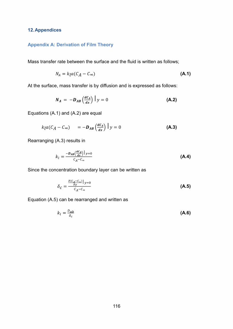
116
12. Appendices
Appendix A: Derivation of Film Theory
Mass transfer rate between the surface and the fluid is written as follows;
∞ (A.1)
At the surface, mass transfer is by diffusion and is expressed as follows:
(A.2)
Equations (A.1) and (A.2) are equal
∞
(A.3)
Rearranging (A.3) results in
∞ (A.4)
Since the concentration boundary layer can be written as
∞
∞ (A.5)
Equation (A.5) can be rearranged and written as
(A.6)

117
Appendix B: Concentration Boundary Layer thickness according to the Film Theory


![[Solutions Manual] Fundamental Os Heat and Mass Transfer [Frank p. Incropera - David p.dewitt]](https://static.fdocuments.us/doc/165x107/55720f17497959fc0b8c8a2b/solutions-manual-fundamental-os-heat-and-mass-transfer-frank-p-incropera-david-pdewitt.jpg)


![( Fundamental of Heat and Mass Transfer by j p Holman 6th Edition[1]](https://static.fdocuments.us/doc/165x107/577cc16c1a28aba71192fbc9/-fundamental-of-heat-and-mass-transfer-by-j-p-holman-6th-edition1.jpg)

