01/2012

Click icon to add picture Click icon to add picture

Click icon to add picture

A Fully Integrated Model for the Optimal Operation of HydroPower Generation

by Francois WeltUniversity of Toronto, Dec. 4, 2012

2

01/2012

Hatch Power and Water Optimization Group

• Engineering Company• Specialized group within Hatch Renewable Power• Experience:

– Over 40 systems implemented– Experience with different types of hydro systems

• Supported by over 9,000 multi-disciplinary engineering professionals worldwide

2

3

01/2012

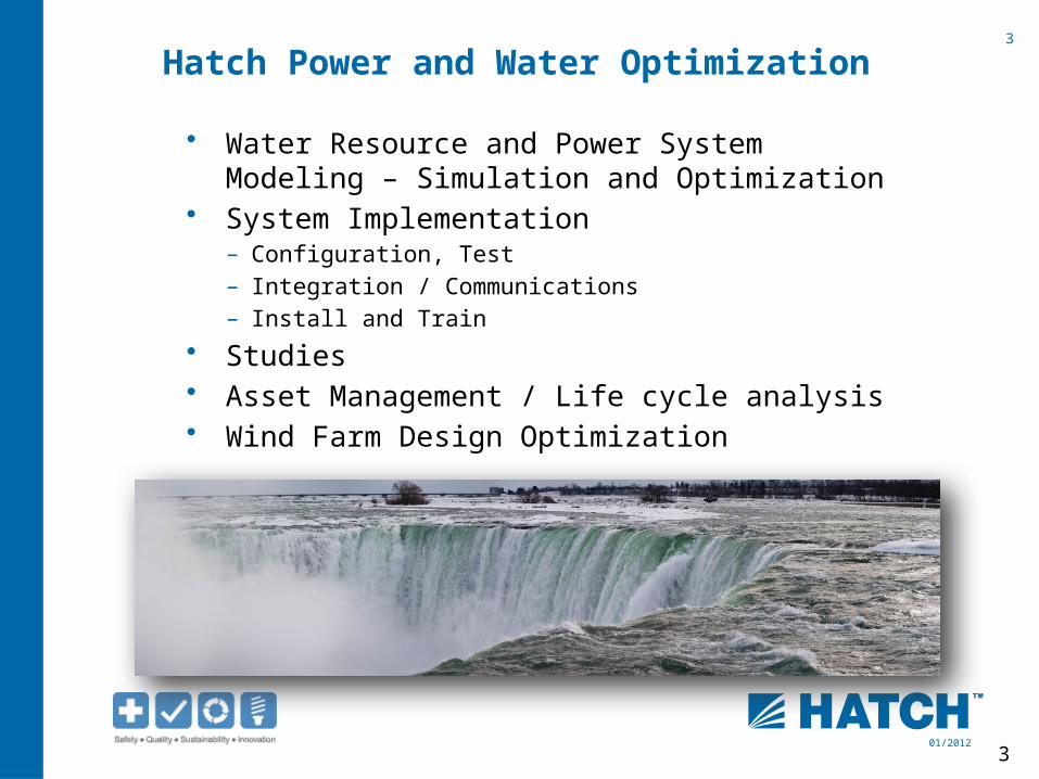
Hatch Power and Water Optimization

• Water Resource and Power System Modeling – Simulation and Optimization

• System Implementation– Configuration, Test– Integration / Communications– Install and Train

• Studies• Asset Management / Life cycle analysis• Wind Farm Design Optimization

3

4

01/2012

Columbia Vista - Integrated Optimization Model

5

01/2012

Hydro Optimization in Generation PlanningConcepts

5

• Make best use of limited hydro resources

• Meet operational constraints• Maximize Profits

– Maximize sales/ Minimize costs– Calculate optimal plant/unit MW– Calculate optimal WL trajectory/

spill releases– Calculate bid curve

Optimization technologies becoming increasingly attractive with improvements in computing speeds/ capabilities

6

01/20126

Optimization StatisticsExamples of potential economic benefits from optimization - Short term operation

0

0.2

0.4

0.6

0.8

1

1.2

1.4

Market Spill Efficiency Head

Ref: “Assessing the Economic Benefits of Implementing Hydro Optimization”,Hydro Review magazine, 1998

Typically, potential improvements between 1 – 5%

7

01/2012

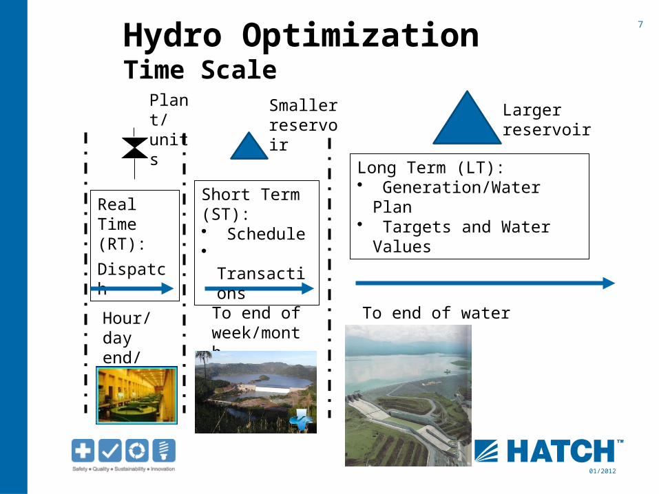
Hydro OptimizationTime Scale

Long Term (LT):• Generation/Water Plan• Targets and Water Values

To end of water year

Short Term (ST):• Schedule•

Transactions

To end of week/month

Real Time (RT):

Dispatch

Hour/day end/

Larger reservoir Smaller reservoir

Plant/ units

8

01/20128

Optimization Problem

Must formulate problem in terms of:• Objective functions• Constraints

• Rules of operation• Physical relations

• Decision Variables

)]}()([Re{ XCostsXvenuesMaxObjectiveTime

0)(int_ XFConstra

Characteristics:• One set of decisions per time step, piece

of equipment• Hydraulic network• Transmission network• Large problem size

9

01/2012

Physical Representation

• Hydraulic Network– Source: Inflow Points– Sink: downstream outlet– Water conveyance/ Flow– Storage– Head (Potential energy) and head loss– Can be bi-directional (gen/pump)

• Electric Network– Source: Generation points– Sink: Load or Market points– Bi-directional– Energy losses

9

10

01/2012

Power Arc Spill Arc

Reservoir Node

RiverReach

Tailwater Junction Node

RiverReach

Inflow Arc

Hydro System Components

11

01/2012

ColumbiaRiver System

12

01/2012

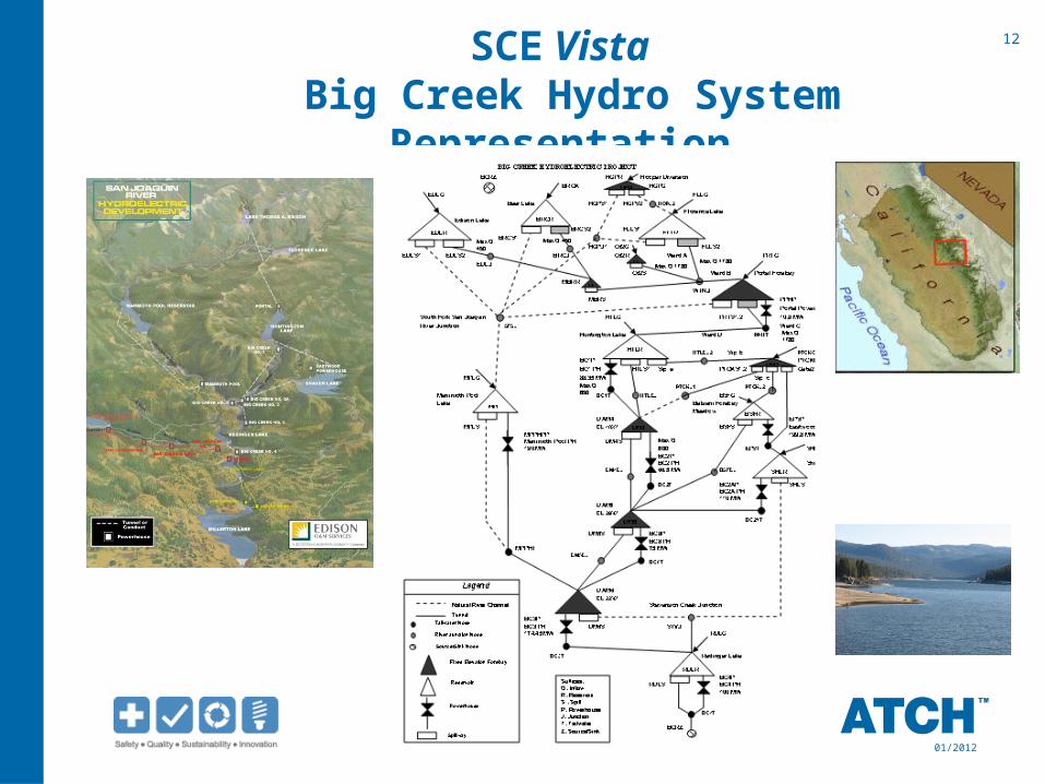
SCE Vista Big Creek Hydro System Representation

13

01/2012

Generation Resource(Hydraulic flow to Electric MW)

14

01/2012

Controlled and Uncontrolled Spillways

15

01/2012

Rock Island Schematic

8 8 8 8 88 8 8 8 8 8 8 88 8 8 88

F FF

Powerhouse Two Powerhouse One

Spillway

16

01/2012

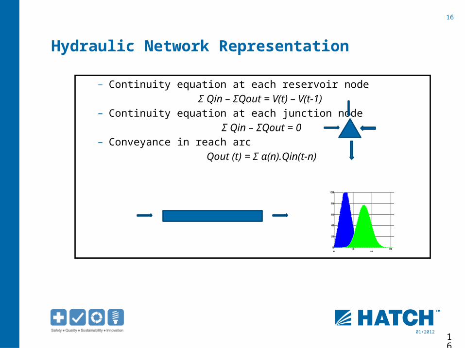
Hydraulic Network Representation

– Continuity equation at each reservoir node

Σ Qin – ΣQout = V(t) – V(t-1) – Continuity equation at each junction node

Σ Qin – ΣQout = 0– Conveyance in reach arc

Qout (t) = Σ α(n).Qin(t-n)

16

17

01/2012

Transmission Area

Load DemandCommitted Transactions

Transaction

XHydro Generation

XD

H

Thermal Generation

Market• Purchase• Sale

Bilateral• Purchase• Sale

T

Wind Wind Generation

18

01/2012

Bus Configuration

Supply AreaRiver 1

River 2

River 3

Plant 3

Plant 4

Plant 5

Plant 6

Plant 1

Plant 2

COB2P

PX(COB2)

COB3S

PX(COB3)

SX(BPA-X)

Bus A

Bus B

COB3P

COB2S

COB1

P

SX(COB1)

X(COB1)

SX(COB2)

BPA1

BPA2

P

SX(PNW2)

X(PNW2)

P

SX(PNW1)

X(PNW1)

X MWY MW

L

MID-C

P

SX(MIDC)

X(MIDC)

Z MW

PSE

SX(PSE)

X(PSE)

W MW

Contract Bus

BPA3

P

SX(PNW3)

X(PNW3)

P

SX(COB3)

“line limits”

“aggregate unit”

“group line limits”

19

01/2012

LT Vista Physical Model

Transmission System

20

01/2012

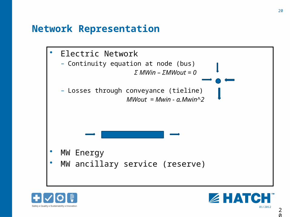
Network Representation

• Electric Network– Continuity equation at node (bus)

Σ MWin – ΣMWout = 0

– Losses through conveyance (tieline)

MWout = Mwin - α.Mwin^2

• MW Energy• MW ancillary service (reserve)

20

21

01/2012

Physical RepresentationReserves and Generation

• Unit/Plant Balance Equation

NON-SPINNING

NON_AGC

LOAD FOLLOW.

MWGENERATION

CONTROL

MAX MW

SPINNING AGC

(Regulating)

TOTAL SPINNING

OPERATING

RESERVE

servesPlantPlant MWMAXMW Re

REG Down

23

01/2012

Joint Optimization

– Energy and A/S markets with price forecasts– Optimal trade-off between energy and A/S

• Spin• Non Spin• Regulation Up• Regulation Down

Energy

• Unused capacity can earn revenues with resulting unused water still sold as energy at a later date

• Some of the unused capacity can be converted into energy when reserve is called (Take)

24

01/2012

Physical Relations: Plants and Units

• Power-flow-head relationship (3-D)

25

01/201225

Spillway Equations

hwl

hwl

Free Overflow

SubmergedFlow

ESill

ESill

Q = Cf · Le · (hwl - Esill)Ef

Q = Co · Le · Open · (hwl - E)Eo

E = Esill or twl

twl

26

01/2012

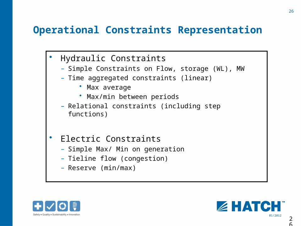
Operational Constraints Representation

• Hydraulic Constraints– Simple Constraints on Flow, storage (WL), MW– Time aggregated constraints (linear)

• Max average• Max/min between periods

– Relational constraints (including step functions)

• Electric Constraints– Simple Max/ Min on generation– Tieline flow (congestion)– Reserve (min/max)

26

27

01/2012

Operational Constraints Representation

28

01/2012

Complexities in Formulation• Uncertainty

– Inflow– Load– Market price

• Hydraulics– Non-linear physical constraints

• generation with cross product (flow * head^a)• Losses (quadratic)• Spill representation

– Spatial/time connectivity

• Discreteness– Start/stop costs– Spinning reserve – Non continuous operating range

• Large Scale – Time dependent decisions (up to 200,000 decision variables / constraints)

Long Term

Short Term

Real Time

29

01/201229

Preferred Schemes for Hydro

Linear Programming• Piecewise linearization• Successive

Linearization• Semi-heuristics

Decomposition• Subproblems• Bender’s cuts• Dynamic Programming• Nonlinear Programming

• Plants are hydraulically and electrically connected– Water conveyance– Load, reserve

• Fixed amount of water over time – strong temporal interdependency

30

01/2012

Long-term Planning

31

01/2012

• Consideration for Future Uncertainty– Stochastic

• Detailed Physical Representation• Simplified Time Definition

– Periods (week(s), month)– Sub-period (peak, off-peak, weekend,…)

• Time Average answers• Based on scenario analysis – consider all cross

correlations

Long Term Model Principles

32

01/2012

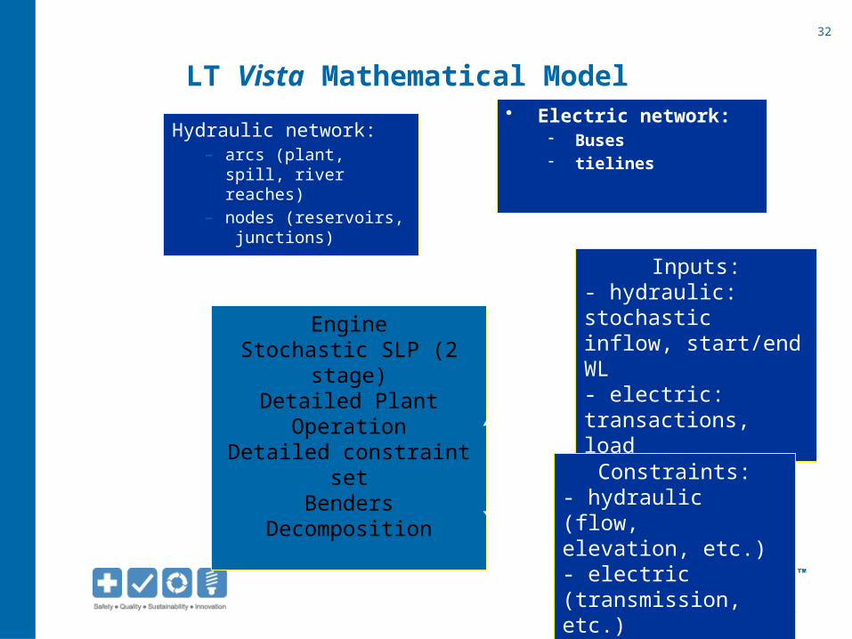
LT Vista Mathematical Model

Hydraulic network:– arcs (plant, spill, river

reaches)– nodes (reservoirs,

junctions)

• Electric network:- Buses- tielines

Inputs:- hydraulic: stochastic inflow, start/end WL- electric: transactions, load

EngineStochastic SLP (2 stage)Detailed Plant OperationDetailed constraint set

Benders Decomposition

Constraints:- hydraulic (flow, elevation, etc.)- electric (transmission, etc.)

33

01/2012

• Two Stage LP• Decomposition Master 1st Period / Future period

subproblem

NOW

Future 1

Future 2

Future 3

Future N

LT Vista Methodology

34

01/2012

• Multi-dimensional Uncertainty -- Inflow, Market and Load

H1

H1_M1

H1_M2

H1_M3

H1_Mm

MarketLoadH1_M2_L1_

H1_M2_L2

H1_M2_L3

H1_M2_Ll

Hydrology

LT Vista Methodology

35

01/2012

LT Vista Time Definition• Period:

– basic model time step (e.g., 1 week)• SubPeriod:

– Peak-off peak (Load duration) aggregation within periods• Time blocks

– constraints tying several periods/subperiods

period

subperiods

Time block

36

01/2012

LT Vista Display – Probabilistic WL

37

01/2012

LT Vista Display – Probabilistic MW

38

01/2012

Short-term Scheduling

39

01/2012

• Deterministic Model• Detailed Physical Representation• Detailed Hourly Time Definition• SLP numerical scheme with piecewise

representation:– MW/Flow relation– Tieline losses

• Unit Dispatch/Unit Commitment Subproblem– Nonlinear Programming– DP

• Spinning reserve allocation subproblem• Integrated handshake with Long Term Model• Market Analysis

Short Term Model Principles

40

01/2012

• Plant Representation based on optimal unit dispatch/ unit commitment around base solution

• Plant Generation function used in SLP• Best Dispatch answers used in scheduling• General LP problem formulation cannot deal with discrete

decisions – unit ON or unit OFF

Unit Dispatch/ Unit Commitment Subproblem

Unit DispatchModel• Snapshot

Non linear analysis

• Fixed Head

Plant 1

Plant 2

Plant N

Non continuous operation

41

01/2012

• Aggregated spill representation• Piecewise linear representation• No flow zone• Sequencing issues – heuristic vs integer set• Stability issues

Spill Allocation

Spill 1

Spill 2

Spill N

42

01/201242

LT – ST Handshake

• Type– Economic

• Seasonal Reservoirs: Value of water in storage applied to end of opt period water levels

• Other Reservoirs/head ponds: Max Target Water Levels at the end of opt period.

– Target Water Levels• Seasonal Reservoirs: LT Target Levels applied to end of opt period water levels• Other Reservoirs/head ponds: Max Target Water Levels at the end of opt period

– Target Flow Releases• Seasonal Reservoirs: LT Target Levels applied to end of opt period water levels• Other Reservoirs/head ponds: Max Target Water Levels at the end of opt period

• Others– meet target water levels defined by user

• Custom– Combination of above

43

01/2012

• Linearized formulation of spinning reserve• Subproblem is to find best unit allocation to meet

spinning reserve requirements• LP Unit representation

Spinning Reserve Allocation Subproblem

0

20

40

60

80

100

120

0 20 40 60 80 100 120

MW Gen

Reserv

e

Operating

Spin

Spin + Reg Down

44

01/2012

Reduction of Problem Size: User Defined Time Grouping

45

01/2012

Total Bus Generation: Comparison between Time Groupings

2 hr4 hr

8 hr

46

01/2012

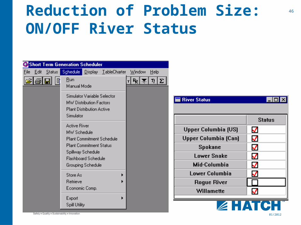
Reduction of Problem Size: ON/OFF River Status

47

01/2012

ST Vista Run Times (866 MHz)

0.0

5.0

10.0

15.0

20.0

25.0

30.0

35.0

0 20000 40000 60000 80000

# of Constraints (row size)

Tim

e (

min

ute

s)

Total Study Time

Hot Starts

Cold Starts

Day Ahead Study Period

48

01/2012

Semi-Heuristic Resolution Schemes

• Plant retirement/commitment• Plant zone resolution• Uncontrolled spillway structure• Semi-heuristic – does not cover all solution space• Perturbation to the LP global problem

Flow

MW

49

01/2012

Price-Volume CurvesMethodology• Cost sensitivity calculation

Time

MW Base

Dev

Storage

Future

$

MWh

50

01/2012

Real Time Dispatch

51

01/2012

• Deterministic Model• Detailed Physical Representation• Detailed sub hourly Time Definition• Detailed Unit Dispatch/Unit Commitment Sub-

problem• Integrated handshake with Short Term Model

Real Time Model Principles

52

01/2012

Unit Commitment – Dispatch Rules

• Minimum unit run time• Minimum unit down time• Maximum number of unit state changes in one time step• Unit start / stop costs• Dynamic unit status eligibility

• Unit availability• Unit available for start• Unit available for shutdown• Unit fixed operations

• Chosen algorithm – Dynamic Programming optimization

53

01/2012

Unit Commitment – DP Formulation

54

01/2012

Unit Commitment – DP Features

• Only states derived from every time step, snap-shot, unit dispatch results are considered

• Only eligible state paths are considered

• Two cost components are evaluated• State transition costs ( unit start / stop costs )• State operation costs ( cost of water to meet generation requirements )

• Objective function – minimize total dispatch cost

55

01/2012

Before

After

Efficiency Gains

56

01/2012

• Future Trends and Developments– Quality of Short Term Schedule

• Robustness/stability– Expansion of market analysis– Handling of uncertainty in Short Term scheduling– Higher flexibility/performance in LT stochastic analysis

Conclusions